Utility of Artificial Neural Networks in Modeling Pan Evaporation in Hyper-Arid Climates


Civil Engineering Department, College of Engineering and Petroleum (COEP), Khaldiya Campus, Kuwait University, P.O. Box 5969, Safat 13060, Kuwait
Water 2020, 12(5), 1508; https://doi.org/10.3390/w12051508
Submission received: 18 April 2020
/
Revised: 18 May 2020
/
Accepted: 21 May 2020
/
Published: 25 May 2020
(This article belongs to the Special Issue The Application of Artificial Intelligence in Hydrology)
Abstract
:Evaporation is the major water-loss component of the hydrologic cycle and thus requires efficient management. This study aims to model daily pan evaporation rates in hyper-arid climates using artificial neural networks (ANNs). Hyper-arid climates are characterized by harsh environmental conditions where annual precipitation rates do not exceed 3% of annual evaporation rates. For the first time, ANNs were applied to model such climatic conditions in the State of Kuwait. Pan evaporation data from 1993–2015 were normalized to a 0–1 range to boost ANN performance and the ANN structure was optimized by testing various meteorological input combinations. Levenberg–Marquardt algorithms were used to train the ANN models. The proposed ANN was satisfactorily efficient in modeling pan evaporation in these hyper-arid climatic conditions. The Nash–Sutcliffe coefficients ranged from 0.405 to 0.755 over the validation period. Mean air temperatures and average wind speeds were identified as meteorological variables that most influenced the ANN performance. A sensitivity analysis showed that the number of hidden layers did not significantly impact the ANN performance. The ANN models demonstrated considerable bias in predicting high pan evaporation rates (>25 mm/day). The proposed modeling method may assist water managers in Kuwait and other hyper-arid regions in establishing resilient water-management plans.
1. Introduction
Evaporation is a key process in hydrology that constitutes the largest water-loss component of the hydrologic cycle. It is defined as the process by which water is transferred from water and land masses to the atmosphere. As water shortages become serious issues, accurate estimations of evaporation rates are crucial, particularly in regions with limited water resources. Sixty-one percent of global precipitation is estimated to be lost through evaporation [1]. For water managers, evaporation rates are indicative of the moisture deficiency status in a given basin. Traditionally, evaporation is estimated using either direct or indirect methods, and measuring evaporation by using pans is one of the most common direct methods used to estimate evaporation [2]. A cylindrical pan is filled with water and exposed to the atmosphere. The free water level change is then monitored over a convenient temporal scale to estimate evaporation.
Although this method can seem appealing, using indirect methods to calculate evaporation is easier and more cost effective. Indirect methods include empirical or semi-empirical models that rely on meteorological measurements. These methods utilize variables such as wind speed, relative humidity, average sunshine hours, solar radiation, and diurnal temperatures to calculate evaporation, along with specific empirical coefficients. The use of site-specific empirical coefficients for evaporation calculations has been reported to have adequate accuracy [3,4]. However, other studies have concluded that some indirect models require data that are difficult to obtain [5,6]. Modelers have combined the aspects of the computational approaches for evaporation calculations into software packages such as the PenPan model and the PenPan-20 models [7,8]. These computer models facilitate evaporation calculations and have been utilized for modeling evaporation rates in numerous past studies with adequate reported accuracies [9].
Despite the satisfactory results of meteorologically based empirical models in predicting evaporation, the use of several meteorological measurements renders such models completely nonlinear. Thus, soft computing and black-box modeling techniques have become attractive research tools for modelers. In most cases, practical and operational forecasts of evaporation rates are more important for water managers than a detailed understanding of evaporation physics. Therefore, these techniques represent suitable evaporation modeling approaches for practical application.
The rapid development of computing technologies since the 1980s has led researchers to adopt soft computing techniques to model time-series data in a variety of disciplines, among which hydrological sciences are no exception. Regarding evaporation modeling, numerous studies have employed artificial intelligence (AI) methods, including artificial neural networks (ANNs), genetic algorithms (GA), support vector regression (SVR), or adaptive neuro-fuzzy inference systems (ANFISs), to forecast evaporation rates [10,11,12]. The ANNs in particular have received extensive attention from researchers [13,14,15,16,17].
Bruton et al. [13] initiated the utility of ANNs in modeling pan evaporation rates. The researchers developed ANNs to model daily pan evaporation at three weather stations in Georgia, USA. The results showed that the ANNs performed slightly better than the multi-linear regression and Priestley–Taylor methods. They also noted a considerable improvement in ANN performance with increased inputs of weather variables. However, they found no significant improvement in ANN performance in response to the calibration of the ANN parameters (e.g., the number of hidden layers). Following this early effort, interest in the application of ANNs to evaporation modeling has expanded. Subsequent studies have mainly focused on examining the efficiency of ANNs in predicting evaporation rates in various climatic zones [11,18]. The ANN models that have been developed are usually considered as site-specific models. This limitation has prompted researchers to examine the global validity of ANN-based evaporation models [19].
Several meteorological measurements have been used to feed ANN models in order to assess their efficiency in predicting pan evaporation [20,21,22]. Keskin and Terzi examined the applicability of ANNs for predicting daily pan evaporation rates at Lake Eğirdir, Turkey [22]. Increasing the number of ANN inputs was found to considerably improve the pan evaporation predictions. Further, ANNs were found to be superior to the well-known Penman method for pan evaporation estimation at the study site.
Due to the limited water resources and harsh environments in arid climate zones, several studies have focused on improving evaporation model efficiency in these zones. In a recent study, a combination of ANN and SVR techniques, in conjunction with wavelet transforms, was implemented to model monthly pan evaporation rates at arid and humid study sites. The capability of the wavelet transforms to enhance the ANN and SVR efficiencies was also assessed. The study concluded that while the wavelet transforms notably improved ANN and SVR performances at the humid site, they did not improve performances at the arid study site. Due the distinct nature of arid region hydroclimatology, temperature and solar radiation were noted as the most precise pan evaporation predictors for black-box models of evaporation in such areas [11].
Nourani et al. [10] examined an ensemble of ANNs in conjunction with other data-driven techniques, including ANFISs, SVR, and other empirical methods, for modeling reference evapotranspiration (ET) rates at 14 meteorological stations in several countries located in different climatic zones. The study used 12 meteorological parameters to feed the ensemble models and applied sensitivity analysis to assess the validity and reliability of the input parameters. While AI-based approaches have shown higher efficiencies for modeling ET rates compared with empirical models, the study concluded that the validity of the input parameters was significantly dependent on the climatic zone where the ensemble model was implemented. Further, the study stressed the need to investigate the feasibility of applying such data-driven approaches in different climatic zones. Dou and Yang [23] investigated the feasibilities of four different AI methods (including ANNs) for modeling daily ET rates in four types of ecosystems (not including arid regions). They demonstrated that AI methods are powerful and efficient tools for predicting ET rates, especially in forest and wetland ecosystems. They recommended that follow-up investigations should further diagnose the suitability of AI methods for predicting ET rates in different climatic zones.
The ANNs have been established as powerful methods for recognizing observed data patterns and have great potential to produce even better results in the future. However, previous studies have not addressed the suitability and applicability of ANN methods for modeling pan evaporation rates in hyper-arid conditions. Climatic conditions in hyper-arid regions have reportedly led to notable deficiencies in the performance of ANNs to model evaporation rates [11]. Therefore, it is necessary to examine the ANN-based modeling approach for modeling pan evaporation rates in such harsh climatic conditions. The present study is the first attempt at investigating the suitability of ANNs to model pan evaporation rates in hyper-arid climates. Specifically, the modeling of daily pan evaporation rates via ANNs at the Kuwait International Airport (KIA) meteorological station in the State of Kuwait was assessed. In addition, a sensitivity analysis of the influences of meteorological parameters on the performance of the ANN models was conducted to determine the parameters that most influenced the models’ efficiency. The results of the current study help to bridge the research gap on the applicability of ANNs in modeling evaporation processes in hyper-arid climatic regions.
2. Materials and Methods
2.1. Study Area
2.1.1. Geography, Water Resources and Climate
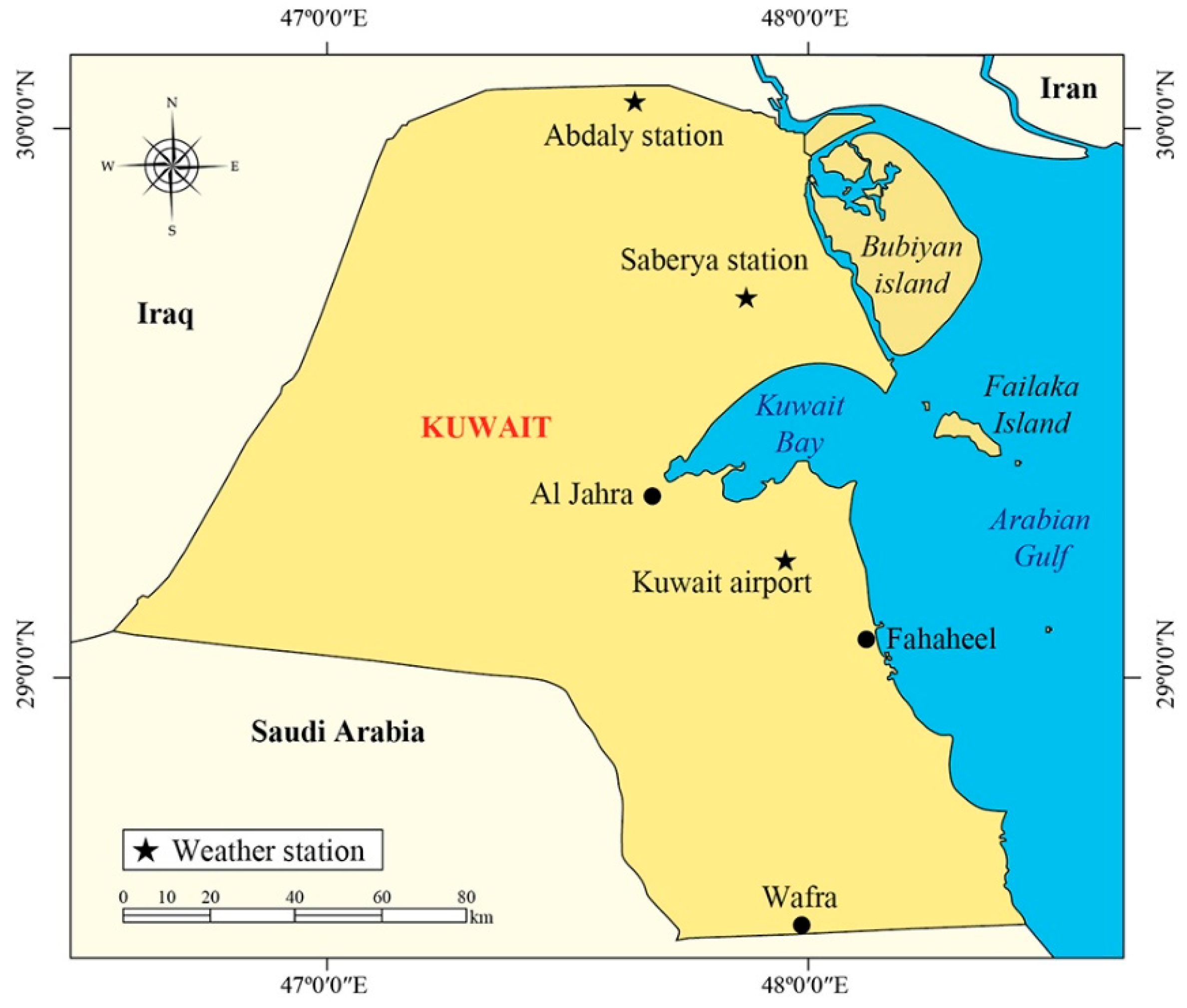
Kuwait is located in the eastern part of the Middle East region between latitudes 28.45° N and 30.05° N and longitudes 46.30° E and 48.30° E (Figure 1). The country occupies a total land area of 17,818 km2 that is mainly deserts and low offshore islands. The country lacks surface water resources such as rivers, lakes, or springs. Groundwater is the sole conventional water resource available. Annual precipitation rates barely exceed 100 mm, with frequent drought seasons having less than 70 mm of annual rainfall. Pan evaporation rates exceed 3500 mm annually. Not surprisingly, the country is considered one of the most arid inhabited regions in the world.
The climate of Kuwait is largely controlled by continental frontal influences, though the oceanographic effects of the Arabian Gulf have some limited influence. Kuwait’s climate is characterized by a hot and dry summer season and a mild to cold winter. Precipitation occurs primarily at the beginning of the winter season and declines afterward. Precipitation peaks again during late spring in the form of isolated thunderstorms. Maximum temperatures exceeding 50 °C have been recorded during the summer months. However, temperatures recorded during the winter rarely drop below the freezing point. The topography of the country is nearly flat, with undulating plains and occasional low hills and depressions. These topographic features do not produce variations in climate within the country. Historical meteorological records collected from various weather stations show minimal variations in recorded precipitation, temperature, humidity, and wind speed. Hence, it is customary to use a dataset from a single station to represent the statewide climatic factors.
2.1.2. Available Data
In this study, the KIA weather station was selected for the necessary meteorological data collection. Due to the continuity of its data records, the station is considered the most suitable station for comprehensive meteorological analyses in the state [24]. The KIA station is a synoptic weather station located at 29.22° N, 47.97° E. Daily precipitation, maximum and minimum temperatures, maximum and minimum relative humidity, average wind speeds, and pan evaporation data are available from January 1993 to July 2015. Wind speeds and air temperatures were collected at a height of 2 m. The average relative humidity can be calculated by taking the arithmetic mean of the maximum and minimum daily measurements. Table 1 summarizes the basic descriptive statistics for the daily meteorological data collected at the station, and the location of the KIA station is illustrated in Figure 1. In addition, pan evaporation and air temperature data are available from the Abdaly and Saberya weather stations, respectively. These datasets will be used to test model generalizability at a later stage to assess the model’s robustness.
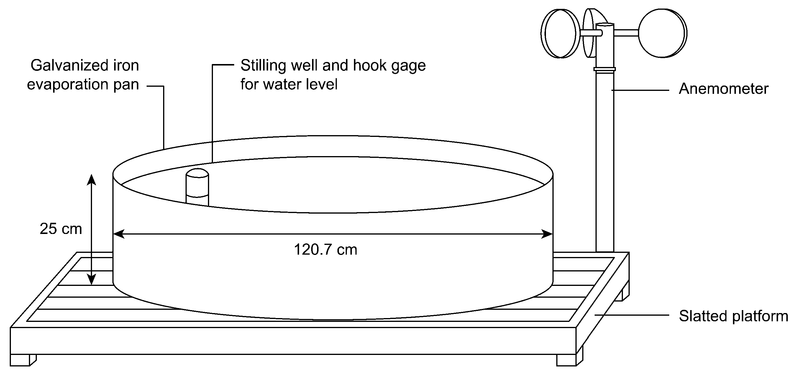
Pan evaporation data were collected using a standard US weather bureau class A pan (Figure 2). The pan is 120.7 cm in width by 25 cm in depth. Just like other pans, the side wall of the pan is exposed to the open atmosphere, which substantially affects the energy balance governing the water inside the pan. Thus, collected pan evaporation data are usually greater than lake evaporation data. Therefore, it is customary to convert pan evaporation measurements to the corresponding lake evaporation equivalent by multiplying the measured pan evaporation data by the pan coefficient. The pan coefficient represents the ratio of lake evaporation to pan evaporation and is always less than one. In the study area of the current study, the measured pan evaporation rates from KIA station have been modeled and verified by several previous studies [25,26,27].
2.2. Artificial Neural Networks
2.2.1. Basic Theory and Architecture
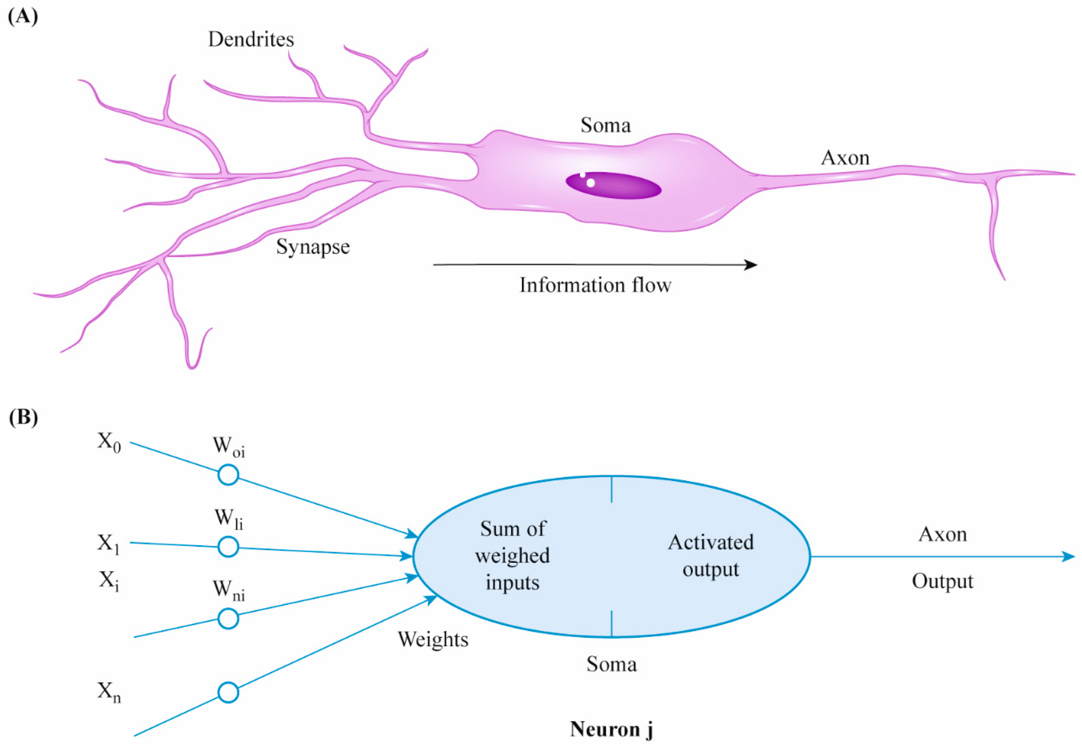
ANNs are sophisticated information processing systems that emulate human intelligence in handling and processing information. They are best known for their capability to model highly nonlinear processes, including pattern recognition problems. The ANNs are basically composed of input, hidden, and output layers that are connected to artificial neurons. These artificial neurons function in a similar way to biological neurons in processing parameters stored in the input layer. Each processed stored parameter is modified via weighting. This weight, frequently referred to as a synaptic weight, functions comparably to a synaptic junction in a biological neuron. Figure 3 provides a schematic representation of information processed by artificial neurons.
Information processing begins by summing the weighted input variables as follows:
where I is the weighted input, i denotes the layer index, j denotes the neuron index, wij is an assigned weight between the ith layer and jth neuron, and xi is the value of the input that is stored in the ith layer. An activation function, f, determines the output of the jth neuron such that:
Sigmoid functions, such as logistic or hyperbolic functions, are commonly used as activation functions. Sigmoid functions are monotonic, bounded, and non-decreasing. These features provide the nonlinearity signature for neural networks [15,28]. Because of the simplicity of computing derivates during the training period using sigmoid functions, such functions have gained popularity for ANN applications.
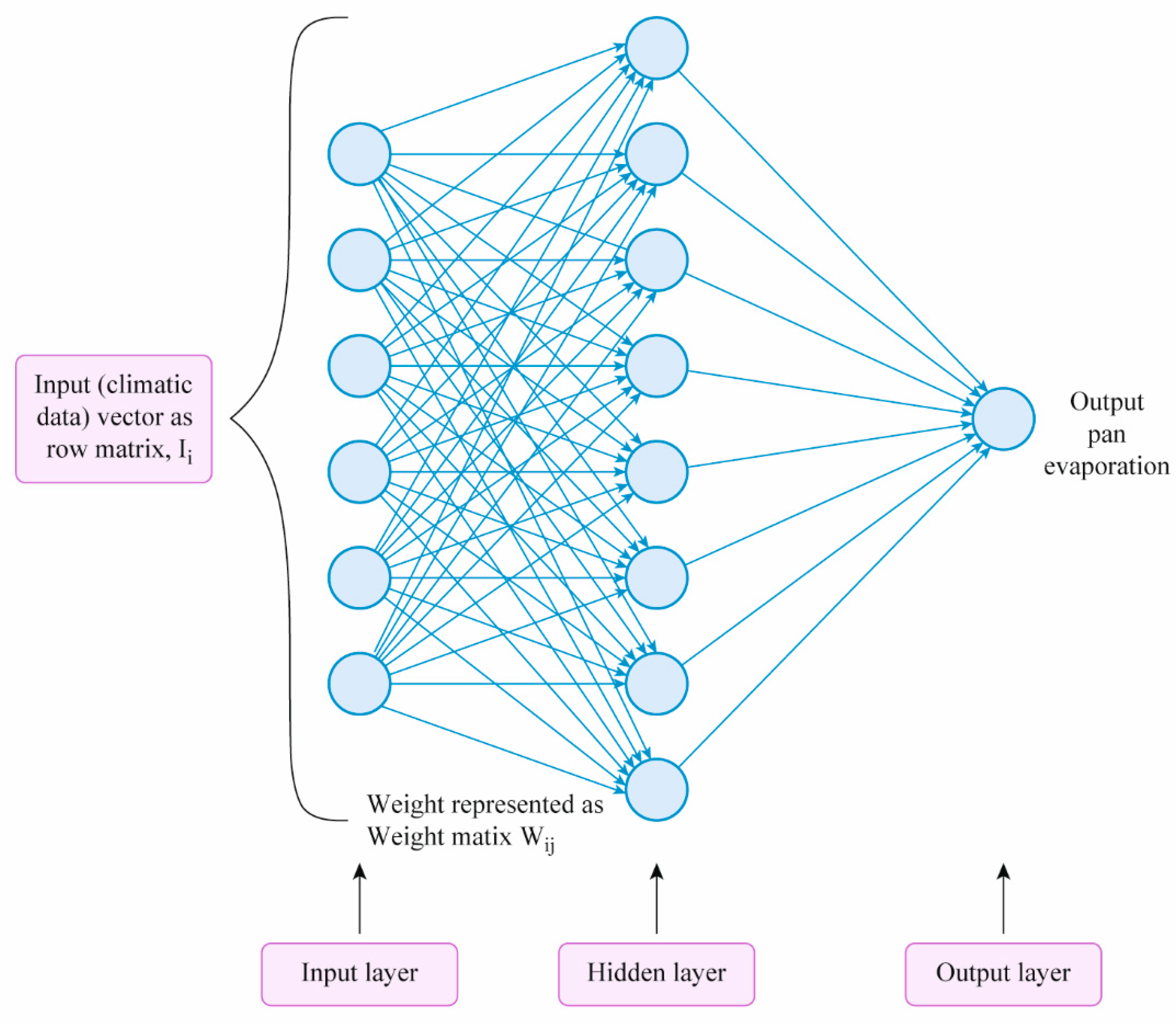
The ANNs can be arranged in layers where information is processed from one layer to the next; in this configuration, they are known as feedforward neural networks (FNNs). The FNNs incorporate the following six elements: the definition of the input layers and number of nodes, activation function selection, the definition of the output layer and number of nodes, hidden layer optimization and number of nodes, training and validation algorithm selection, and performance evaluation. Figure 4 demonstrates the architecture of the FNN network used for modeling pan evaporation in this study.
2.2.2. Data Pre-Processing
To enhance the ANN performance, the daily pan evaporation data (targets) are normalized to a 0–1 range. The ANNs are sensitive to the absolute values of the targets. Thus, the normalization procedure assures better model performance. The activation function processes input variables through the middle layer of the network; this function causes minimal changes to the variable weights when values are in the 0–1 range. Rao and Rao [29] reported that artificial neurons are more responsive to values near 0.5. The 0–1 normalization for pan evaporation data has been employed in past studies and generated satisfactory results [30,31]. The normalization is then eliminated from the simulated output to enable comparisons with the raw pan evaporation data.
2.2.3. Training Algorithms
Optimal input variable weights should be identified to achieve the best match between the input variables and the target variable. The training (learning) processes utilize optimization algorithms to minimize errors between the ANN output and the target output. In this study, The Levenberg–Marquardt (LM) training algorithms were employed for this purpose.
The LM method is commonly utilized for time-series network training and performance evaluation [32,33,34,35]. This approach employs a form of the Gauss–Newton algorithm that determines the minima function and subsequently optimizes the solution. It also employs an approximation of the Hessian matrix based on the previous work of Bishop [36]. In the current study, the LM algorithm was used to optimize the variable weights through an iterative process.
The Hessian matrix is approximated as follows:
where w denotes the weight vector, denotes the Jacobian matrix, denotes the transpose matrix of , denotes the learning parameter, denotes the identity matrix, and denotes the error vector of the network.
2.3. Sensitivity Analysis
Different combinations of meteorological inputs were used to assess the ANNs’ efficiency in modeling pan evaporation. Because of the high temperatures in the study area, the mean temperature variable was used as the basic predictor for pan evaporation. Subsequently, average daily temperature was paired with average wind speed and average relative humidity to form different input combinations. Table 2 lists the meteorological variable combinations that were used as inputs for the ANN models. This sensitivity analysis was performed to demonstrate the effects of various meteorological variables in improving ANN performance. The number of hidden layers for the ANN was set to 10 to provide a common base for models’ comparison.
2.4. Validation and Statistical Assessment
To assess the ANNs’ effectiveness in modeling pan evaporation in the study area, this study adopted the conventional approach of chronologically dividing the data into a training period and a validation period. A subset of 80% of the data was selected for ANN training, while the remaining 20% was used for model validation. In this study, four statistical performance metrics were employed to assess model performance: the Pearson correlation coefficient, the coefficient of determination (R2), the mean absolute error (MAE), and the Nash–Sutcliffe coefficient (NS).
The Pearson correlation coefficient is a well-known statistical metric that provides an indication of the linear association between the measured and modeled data. The coefficient of determination (R2) provides a deeper insight into the extent of the association between the measured and the modeled data. R2 represents the square of the Pearson correlation coefficient. However, unlike the Pearson correlation, R2 does not provide a direct measurement of how reliable the predictions are; instead, it indicates the quality of a predictor that could potentially be constructed from the given model. This parameter varies between 0 and 1; 0 represents the absence of any statistical association, and 1 indicates an exact correlation between the modeled and measured data.
The MAE was also used to assess the performance of the ANN model. It provides an objective indication of the variations between the modeled and measured targets. The NS coefficient, a commonly used metric that is used to evaluate the performance of hydrological models [37], was also employed in this study. The NS coefficients vary between −∞ and 1. A value less than 0 implies that the arithmetic mean of the measured data represents a more reliable prediction than the modeled values.
3. Results and Discussion
3.1. ANNs Modeling Results
This study investigated the suitability of ANNs for modeling pan evaporation rates in hyper-arid environments. To determine an optimal combination of input variables for the ANN model, the predictions of the model using different combinations of input variables were compared with measured values from the KIA monitoring station. Table 3 lists the statistical performance metrics for the ANN using the input combinations described in Table 2. Highlighted values in Table 3 represent the best performing statistical metric values in the training and validation periods. Model 1, in which only mean daily temperature data were used as inputs, served as the baseline ANN model in this study. This baseline model exhibited satisfactory efficiency in modeling pan evaporation, achieving NS values of 0.778 and 0.405 in the training and validation periods, respectively. Model 1′s R2 values also indicate its adequacy for predicting pan evaporation rates.
Including wind speed as an input variable enhanced the performance of model 2 in predicting pan evaporation rates. This is clearly reflected in the statistical evaluations, particularly model 2′s much higher NS value (compared with that of model 1) in the validation period. The improvement in the ANN’s performance due to the inclusion of wind speed is considered logical because it reflects the role of wind speed in evaporation. Wind speed facilitates the evaporation process by removing evaporated water from evaporation surface and thus maintains the vertical vapor pressure gradient between the evaporation surface and the overlying air. According to Fick’s first law, evaporation is a diffusive process. Thus, this vapor pressure gradient is essential for evaporation to occur.
Model 3, which includes the average relative humidity and average temperature as input variables, represented a smaller improvement over model 1 than did model 2. Relative humidity measures the amount of water vapor in the air relative to the amount needed for water vapor saturation. A higher relative humidity indicates a higher concentration of moisture water above the evaporating surface. Subsequently, decreased evaporation will occur, as evaporation is strongly dependent on the vapor pressure gradient. However, the role of the relative humidity variable in improving the ANN model’s performance was found to be less than that of wind speed.
Model 4, which combined all of the meteorological input variables, represented pan evaporation rates approximately as effectively as model 2. This was reflected in the validation period NS values of 0.755 and 0.638 for models 2 and 4, respectively. However, in model 4, the excessive meteorological inputs resulted in model overfitting. To confirm the overfitting in model 4, performance metrics from the training and validation periods of all models were compared. The NS value for model 4 in the training period was found to be the largest. However, in the validation period, the NS value for model 4 ranked below that of model 2. This inconsistency in NS metric performance implies that model 4 may have been overfitted during the training period. Therefore, the use of excessive inputs should be avoided when using ANNs to model pan evaporation. The correlation and R2 values shown in Table 3 indicate that ANN models can reliably predict pan evaporation rates. Specifically, models 2 and 4 demonstrated strong correlations between the measured and modeled pan evaporation values, with correlations and R2 values exceeding 0.8 in the validation period. However, models 1 and 3 demonstrated less effective modeling capabilities based on their correlations and R2 values.
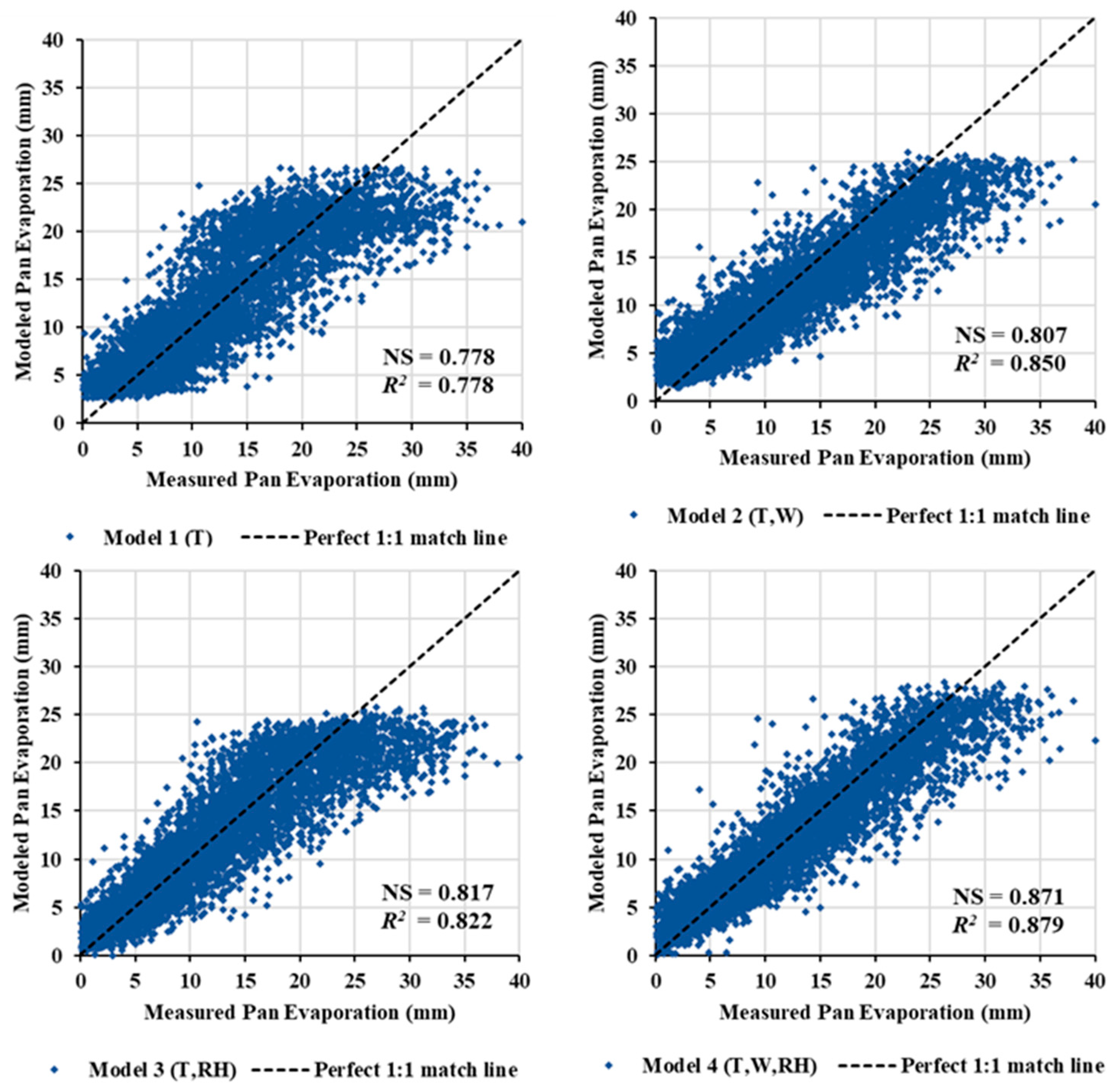
Figure 5 shows the modeled versus the measured pan evaporation values plotted with respect to a perfect 1:1 match line in the training period. This reflects the models’ performance with respect to prediction randomness. In Figure 5, it is evident that all constructed ANNs were able to model evaporation rates in the training period without noticeable bias, except under high evaporation rates (> 25 mm/day). This finding is demonstrated by the random scattering of modeled results above and below the 1:1 match line for measured pan evaporation rates of < 25 mm/day. Significant biases within all the models were noted for high evaporation rates (> 25 mm/day). The ANN models continually underestimated pan evaporation rates within the upper range of measured pan evaporation rates. This may indicate that a bias correction is necessary for trained ANNs applied at high evaporation rates to enhance the models’ reliability.
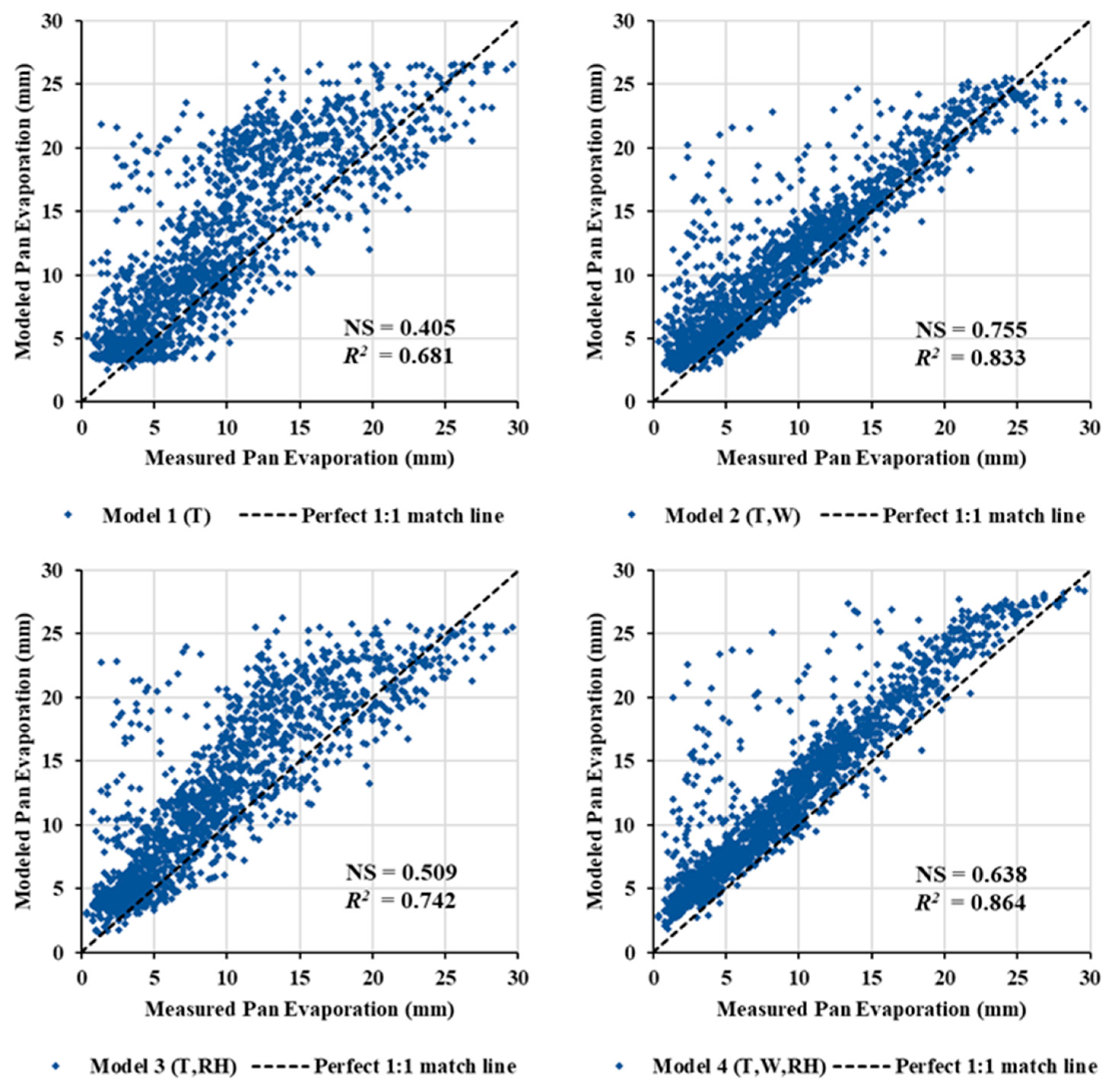
The biases of the ANN models’ performance were much lower during the validation period (Figure 6). Except for model 4, Figure 6 shows a random scattering of results above and below the 1:1 line, thus indicating the appropriate randomness representation in the models’ predictions. This outcome is likely attributable to the less frequent occurrences of higher pan evaporation rates within the validation period. The validation period covered a 20% subset of the entire data range. Consequently, fewer instances of high evaporation rates occurred, which led to reductions in the models’ biases. Model 4, however, presents a different pattern and appears to consistently overestimate pan evaporation rates. The overfitting problem may underlie this outcome.
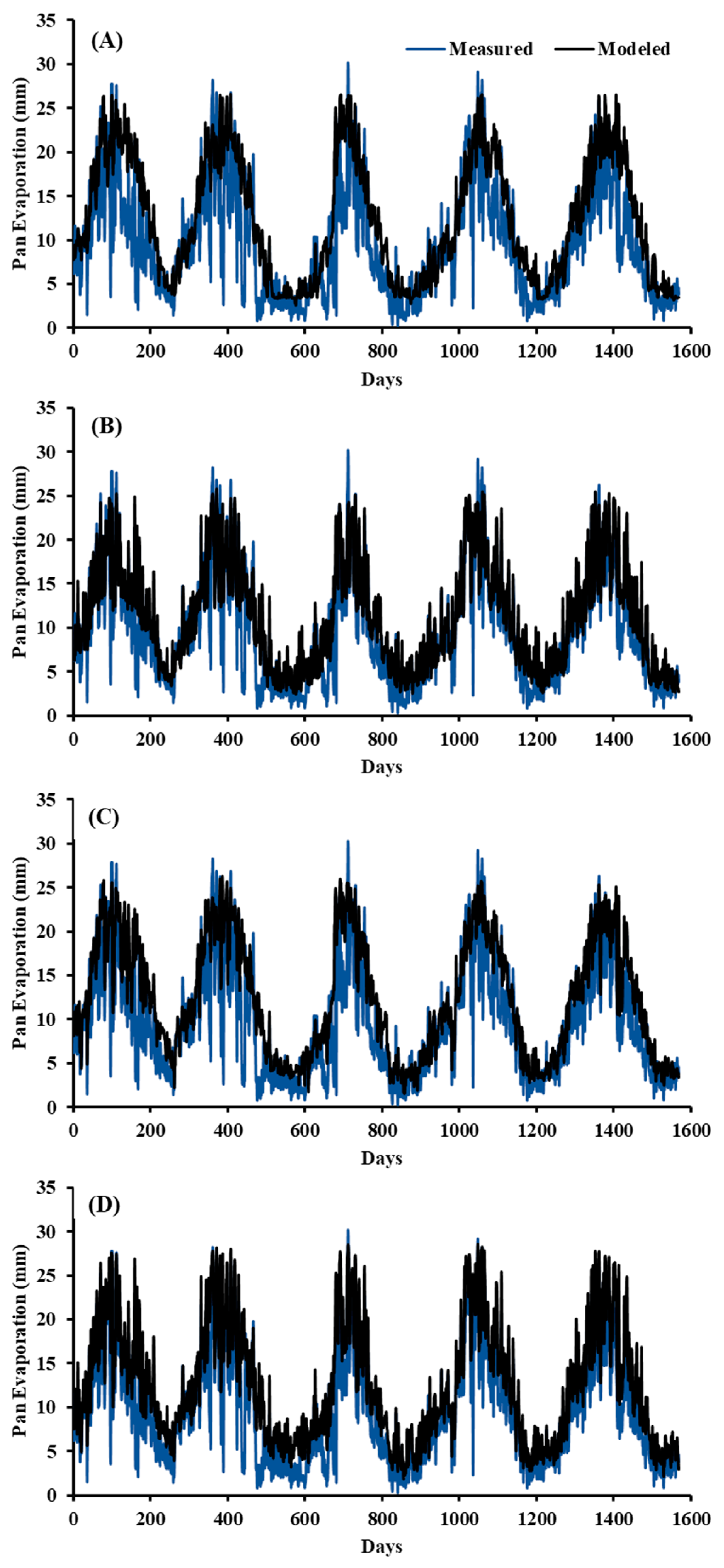
Figure 7 presents the measured and modeled pan evaporation rates over time for the validation period. The modeled time-series satisfactorily reflect the measured time-series data. Specifically, long-term trends and seasonal patterns are well-represented. Discrepancies between the measured and modeled pan evaporation values were found to be minimal. Indeed, the ANN model’s capacity to represent long-term trends in pan evaporation rates is a remarkable feature of the model and suggests that ANNs can capture the long-term variations in pan evaporation rates that could be induced by climate change.
It essential to investigate the effects of ANN architecture on the models’ performance. Sensitivity analysis results regarding the number of hidden layers used to build the ANN models are presented in Figure 8. Each model began with 10 hidden layers, which were then increased by increments of 10 up to 60 hidden layers. Modeled pan evaporation rates were assessed based on the NS coefficient. The NS values presented in Figure 8 were calculated for the entire data range. Variations in the number of hidden layers were found to have a minimal effect on the models’ performance. This finding agrees with that of Bruton et al. [13], who conducted the same sensitivity analysis for daily pan evaporation rates at weather stations located within humid areas. The ANN parameters that were used for constructing the best performing model in the validation period (model 2) are listed in Table 4.
3.2. Model Generalizability
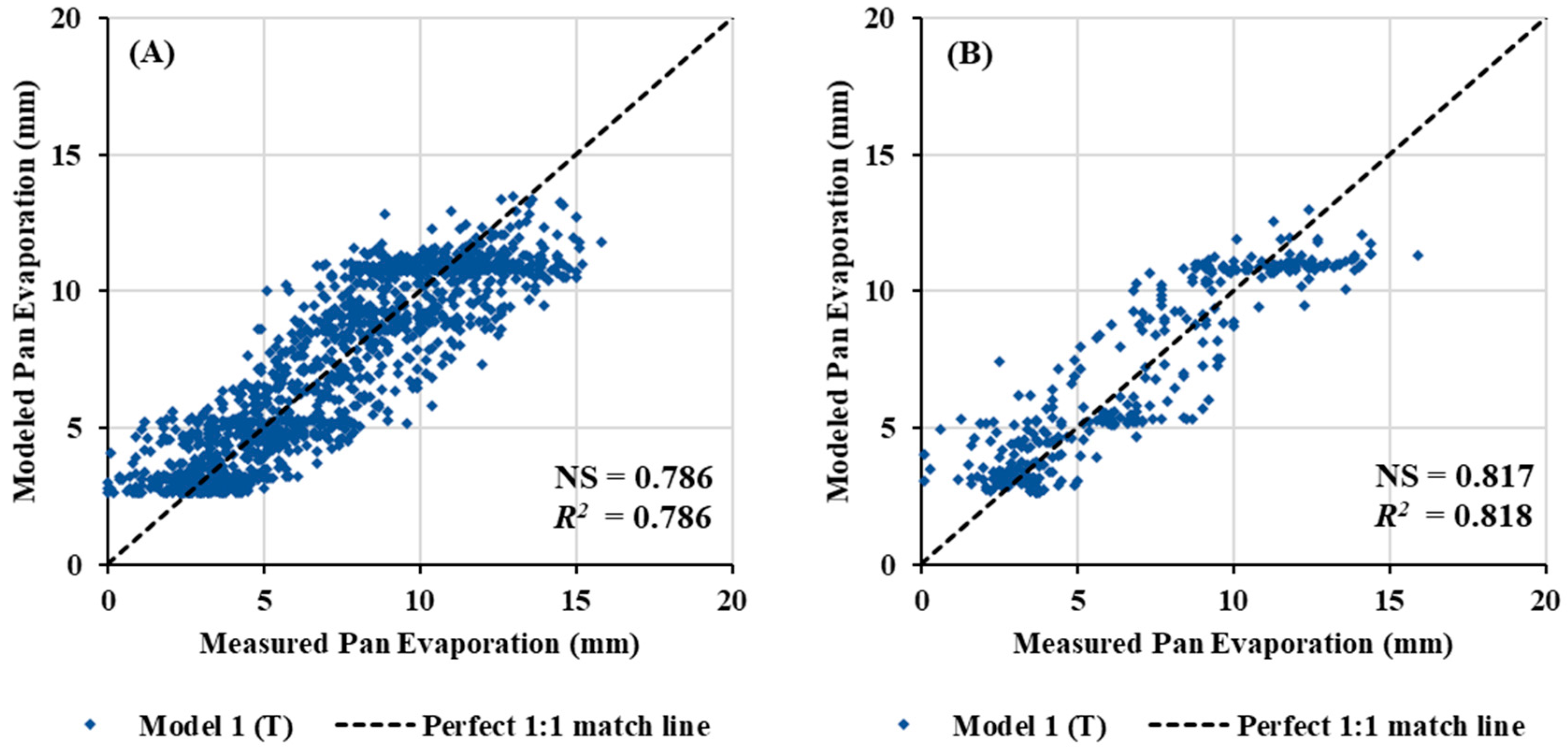
To confirm the generalizability of the results, the ANN-based model was used to model the daily pan evaporation rates at Abdaly weather station. Due to the recent installation of the station, the time span of the data was 5 years. However, this time span is considered adequate for model testing purposes. The base ANN model (model 1) was used to model the pan evaporation rates. The required air temperature data were available from Saberya weather station for the same data period. The same model parameters as those listed in Table 4 were used to construct the model. Figure 9 shows the modeled versus measured pan evaporation data for the testing station in the training and validation periods with corresponding evaluation metrics. Evidently, the simulation results demonstrated similar features as the obtained modeling results for the KIA station. The model exhibited the same modeling efficiency with comparable values for the statistical metrics. This adds an additional strength feature for the developed ANN model. It is worth noting here that the Abdaly station is approximately 110 km to the north of the KIA station; however, due to the flat topography of the State of Kuwait, the spatial variability of the meteorological measurements made within the state is considered minimal [38]. The mobility of the presented model is limited to areas with similar climatic conditions. Recalibration and reassessment of the model parameters should be conducted if the model were to be applied in other locations with different climates. Further, it is recommended that a model generalizability assessment should be extended for other ANN models that are listed in Table 2. This will require additional meteorological data collection from the Abdaly station.
3.3. Agreement with Past Studies
The results of the current study suggest that ANNs are suitable for modeling pan evaporation processes in hyper-arid climates. Hyper-arid climates possess unique hydrometeorological regimes characterized by scarce water resources, bare vegetation cover, and high evaporation rates. According to the United Nations Food and Agriculture Organization, hyper-arid climates are defined as regions where the annual precipitation does not exceed 3% of the annual evaporation [39]. The State of Kuwait receives 115 mm of average annual precipitation, while the average annual pan evaporation exceeds 4000 mm. Previous efforts that employed ANNs in estimating pan evaporation rates have not largely considered such models for use in such extremely harsh environments.
In the present study, ANNs were found to be generally capable of modeling pan evaporation in hyper-arid climates and in achieving performances comparable with those of ANN models applied in other climatic regimes. The performances of ANNs in a hyper-arid climate were found to be similar to those observed in previous studies that investigated the applicability of ANNs for modeling evaporation rates in comparable climatic conditions. Piri et al. [40] were among the first to attempt to utilize ANNs for modeling pan evaporation rates in arid and semi-arid climates. They reported satisfactory performances for ANNs applied at a study site located in southeast Iran. Their study reported an R2 of 0.93 for an ANN model with an optimized combination of meteorological inputs. In the present study, the best R2 value achieved was 0.864 during the validation period, as shown in Table 3. This implies that ANN-based models are slightly less effective in hyper-arid climates. Additionally, the application of ANN models at the arid study site yielded the same prediction bias reported in the present study regarding high pan evaporation rates. However, in hyper-arid climates, the frequency of such high pan evaporation rates is greater, resulting in a slightly lower model performance.
The results of the current study are also comparable to those concerning other artificial intelligence methods applied in similar climatic conditions. Moghaddamnia et al. [41] applied the ANFIS method in the same study area as Piri et al. [40] in southeast Iran and reported an R2 value of 0.91 for their best-performing ANFIS model during the validation period, compared with an R2 value of 0.864 found in the present study. However, the same prediction bias was also observed for the ANFIS model. Thus, future research should attempt to further improve AI techniques to allow more reliable predictions for high pan evaporation rates. A bias-correction method may represent an appropriate approach in this regard. In addition, future studies might consider other meteorological variables for which data were not available at the KIA study site to construct ANN models. However, the results of the present study show that the application of ANNs for modeling pan evaporation yielded satisfactory and reliable predictions.
3.4. Comparisons with Conventional Evaporation Estimation Methods
It is essential to assess ANN efficiency to model measured pan evaporation in light of practical evaporation estimation methods. In this study, the best performing ANN model in terms of MAE metric (model 2) estimated a daily MAE of 2.015 mm, which is equal to 735.5 mm/year. Abusada [42] compared class A pan evaporation data that were collected from the KIA station from 1962 to 1977 to theoretical calculations of evaporation estimation by using the Penman method at the same station for the same period. The comparisons showed that the Penman method estimated an annual evaporation rate of 2630 mm, while the measured annual pan evaporation for the same period was 3540 mm. Thus, the error that resulted from applying the Penman method is 910 mm/year. Accordingly, the error in pan evaporation estimation using the ANN modeling approach from the current study is approximately 20% less than the error estimated by the Penman method for the same weather station. Despite being among the best performing practical methods for estimating evaporation in an arid climate [43], the Penman method was found to underperform the ANNs in this study. However, this underestimation resulting from a physically based methodology such as the Penman method can be justified. The wall of the evaporation pan intercepts additional solar radiation and enhances heat exchange with the surrounding atmosphere [44]. Thus, physically based models cannot be used for directly estimating pan evaporation.
It is also essential to compare ANN model performance with other practical models by addressing the issue of the pan wall’s contribution to heat exchange. Though it has been reported in previous studies that ANN-based models are superior to such practical models [45], future studies focusing on evaporation modeling in hyper-arid climates should work on bridging this research gap, specifically in unique hydrometeorological systems in hyper-arid regions. This will require detailed data collection of other meteorological variables such as sunshine hours, vapor pressures, and pan wall material properties. A key advantage of using the ANN-based model is that it does not have such detailed data requirements. In this study, efficient performance of the pan evaporation predictions was achieved using widely available meteorological data (air temperatures, wind speeds, and relative humidity). However, unlike physically based methods, the ANN-based model does not reflect the actual physics of the evaporation process. This limits ANN-based model application to practical purposes that do not require theoretical investigations of the evaporation process.
3.5. Model Shortcomings
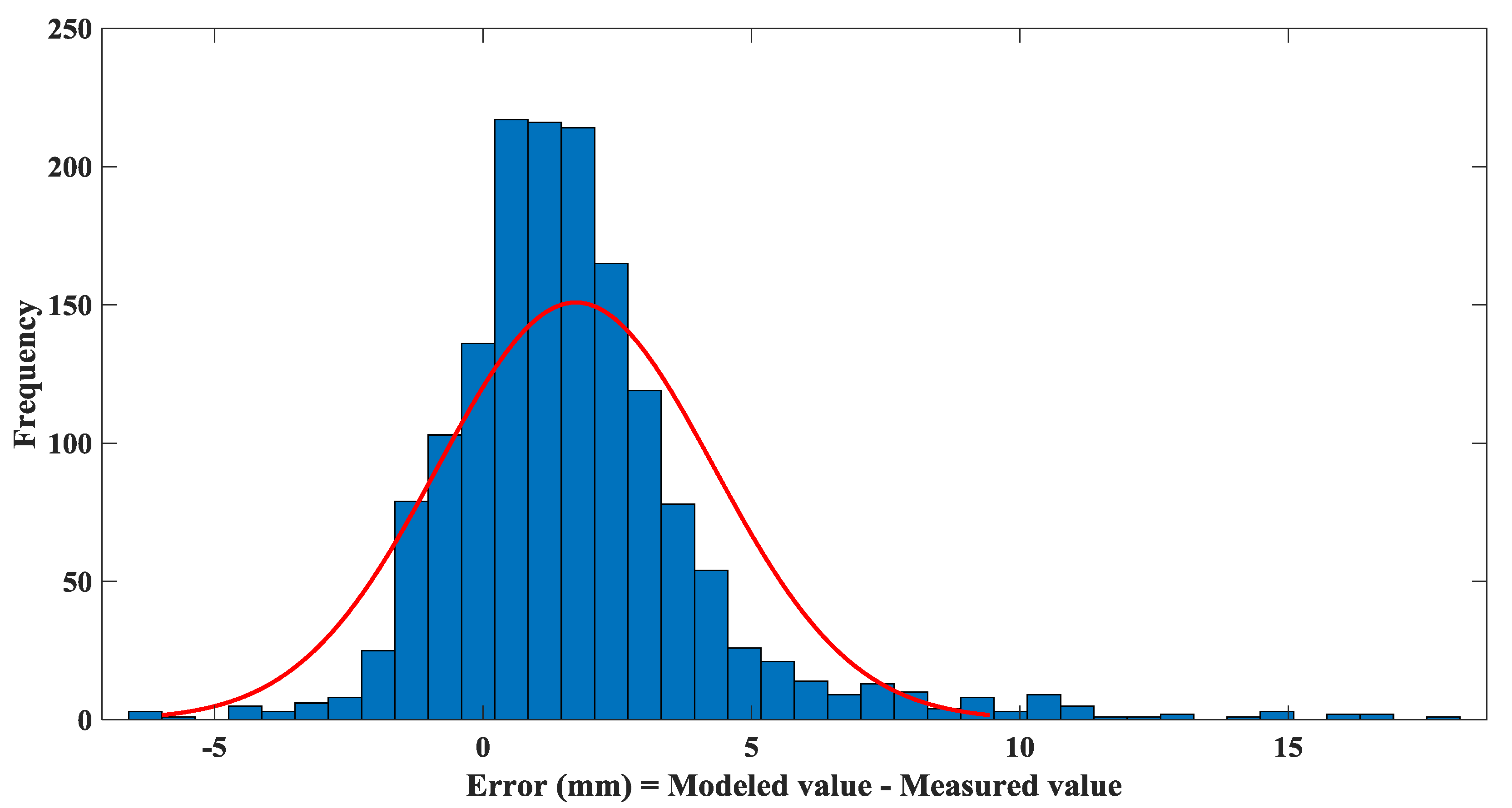
Despite the soundness of ANN-based models’ application, there are minor model drawbacks that should be considered. First, the selection of the number of hidden layers for model construction and sensitivity analysis is quite arbitrary. The optimal number of hidden layers is obtained by trial and error procedures. Thus, there is no guarantee that the computed optimal number of hidden layers represents the global optimal solution. Second, the ANN model may fail in forecasting due to the overfitting issue. This drawback occurs in cases when networks in the training phase try to fit the noise component of data instead of fitting a data trend. In this case, a considerable drop in the validation phase will happen. In general, the tendency of model overfitting is driven by feeding the model with excessive inputs. It is crucial to examine the model predictions to check for this common problem and to ensure the robustness of the results. To achieve this goal, the error distribution within the validation period was plotted for the best performing model in the validation period in this study (model 2). The normally distributed error shown in Figure 10 indicates that the developed ANN model is objectively performing with positive and negative errors that are normally distributed across the zero-error point. It is worth noting here that the distribution curve is slightly skewed to the right. This skewness is driven by the likelihood of the model to overestimate pan evaporation values. However, this deficiency is considered acceptable and does not violate the soundness of the model.
4. Conclusions
This study has investigated the applicability of ANNs in modeling pan evaporation rates in hyper-arid climates. Daily pan evaporation data and other necessary meteorological measurements were collected from the KIA, Saberya, and Abdaly weather stations in Kuwait. Different combinations of meteorological data inputs to the ANNs were examined to optimize the ANN structure to replicate the measured data. Mean air temperatures and average wind speeds were the meteorological factors that most affected the model performance. This study also found that feeding excessive meteorological data to ANNs may result in model overfitting and consequently low generalizability of the results. The ANN-based model was tested at the Abdaly station to assess the model’s mobility. The results showed that model generalizability can be achieved within the study area, however, caution should be taken if the model were to be used in different climatic conditions. Statistical performance metrics showed that the ANNs are generally robust modeling tools for modeling daily pan evaporation fluctuations in hyper-arid climatic settings. Further, a sensitivity analysis showed that variations in the number of hidden layers in the ANNs had a minimal effect on the model performance.
The ANN-based pan evaporation models employed at the study site exhibited notable biases in predicting high rates of pan evaporation (>25 mm/day). This problem was reported by previous studies that evaluated models in less arid climates. However, this bias is exacerbated in hyper-arid climates due to the higher frequency of high evaporation rates. Future research efforts should focus on enhancing the reliability of ANNs in making pan evaporation predications in such cases. This requires employing bias correction techniques to overcome the observed bias in predictions of high evaporation rates. Moreover, additional meteorological measurements (e.g., vapor pressure, sunshine hours, and incoming solar radiation) should be considered as ANN inputs. These measurements are important in developing physical evaporation models. Thus, they could have a great potential in improving ANNs’ prediction efficiency in hyper-arid climates. The results of this study build on previous tests of the suitability of ANNs for modeling both hydrological processes in general and for evaporation processes in various climatic regions. Advancing our understanding of evaporation dynamics is crucial for establishing resilient water-management plans, especially in hyper-arid regions that suffer from serious water shortage risks.
Funding
This research received no external funding.
Conflicts of Interest
The author declares no conflict of interest.
References
- Chow, V.T.; Maidment, D.R.; Mays, L.W. Applied Hydrology; McGraw-Hill: New York, NY, USA, 1988; ISBN 0070108102. [Google Scholar]
- Stanhill, G. Is the Class A evaporation pan still the most practical and accurate meteorological method for determining irrigation water requirements? Agric. For. Meteorol. 2002, 112, 233–236. [Google Scholar] [CrossRef]
- Irmak, S.; Haman, D.Z.; Jones, J.W. Evaluation of class A pan coefficients for estimating reference evapotranspiration in humid location. J. Irrig. Drain. Eng. 2002, 128, 153–159. [Google Scholar] [CrossRef]
- Frevert, D.K.; Hill, R.W.; Braaten, B.C. Estimation of FAO evapotranspiration coefficients. J. Irrig. Drain. Eng. 1983, 109, 265–270. [Google Scholar] [CrossRef]
- Rosenberry, D.O.; Winter, T.C.; Buso, D.C.; Likens, G.E. Comparison of 15 evaporation methods applied to a small mountain lake in the northeastern USA. J. Hydrol. 2007, 340, 149–166. [Google Scholar] [CrossRef]
- Burman, R.D. Intercontinental comparison of evaporation estimates. J. Irrig. Drain. Div. 1976, 102, 109–118. [Google Scholar]
- Rotstayn, L.D.; Roderick, M.L.; Farquhar, G.D. A simple pan-evaporation model for analysis of climate simulations: Evaluation over Australia. Geophys. Res. Lett. 2006, 33. [Google Scholar] [CrossRef] [Green Version]
- Yang, H.; Yang, D. Climatic factors influencing changing pan evaporation across China from 1961 to 2001. J. Hydrol. 2012, 414, 184–193. [Google Scholar] [CrossRef]
- Yang, H.; Li, Z.; Li, M.; Yang, D. Inconsistency in Chinese solar radiation data caused by instrument replacement: Quantification based on pan evaporation observations. J. Geophys. Res. Atmos. 2015, 120, 3191–3198. [Google Scholar] [CrossRef]
- Nourani, V.; Elkiran, G.; Abdullahi, J. Multi-station artificial intelligence based ensemble modeling of reference evapotranspiration using pan evaporation measurements. J. Hydrol. 2019, 577, 123958. [Google Scholar] [CrossRef]
- Qasem, S.N.; Samadianfard, S.; Kheshtgar, S.; Jarhan, S.; Kisi, O.; Shamshirband, S.; Chau, K.-W. Modeling monthly pan evaporation using wavelet support vector regression and wavelet artificial neural networks in arid and humid climates. Eng. Appl. Comput. Fluid Mech. 2019, 13, 177–187. [Google Scholar] [CrossRef] [Green Version]
- Rezaie-Balf, M.; Kisi, O.; Chua, L.H.C. Application of ensemble empirical mode decomposition based on machine learning methodologies in forecasting monthly pan evaporation. Hydrol. Res. 2019, 50, 498–516. [Google Scholar] [CrossRef]
- Bruton, J.M.; McClendon, R.W.; Hoogenboom, G. Estimating daily pan evaporation with artificial neural networks. Trans. ASAE 2000, 43, 491. [Google Scholar] [CrossRef]
- Sudheer, K.P.; Gosain, A.K.; Ramasastri, K.S. Estimating actual evapotranspiration from limited climatic data using neural computing technique. J. Irrig. Drain. Eng. 2003, 129, 214–218. [Google Scholar] [CrossRef]
- Zanetti, S.S.; Sousa, E.F.; Oliveira, V.P.; Almeida, F.T.; Bernardo, S. Estimating evapotranspiration using artificial neural network and minimum climatological data. J. Irrig. Drain. Eng. 2007, 133, 83–89. [Google Scholar] [CrossRef]
- Khoob, A.R. Artificial neural network estimation of reference evapotranspiration from pan evaporation in a semi-arid environment. Irrig. Sci. 2008, 27, 35–39. [Google Scholar] [CrossRef]
- Sudheer, K.P.; Gosain, A.K.; Ramasastri, K.S. A data-driven algorithm for constructing artificial neural network rainfall-runoff models. Hydrol. Process. 2002, 16, 1325–1330. [Google Scholar] [CrossRef]
- Traore, S.; Wang, Y.-M.; Kerh, T. Artificial neural network for modeling reference evapotranspiration complex process in Sudano-Sahelian zone. Agric. Water Manag. 2010, 97, 707–714. [Google Scholar] [CrossRef]
- Kumar, M.; Raghuwanshi, N.S.; Singh, R. Artificial neural networks approach in evapotranspiration modeling: A review. Irrig. Sci. 2011, 29, 11–25. [Google Scholar] [CrossRef]
- Kişi, Ö. Daily pan evaporation modelling using multi-layer perceptrons and radial basis neural networks. Hydrol. Process. Int. J. 2009, 23, 213–223. [Google Scholar] [CrossRef]
- Tabari, H.; Marofi, S.; Sabziparvar, A.-A. Estimation of daily pan evaporation using artificial neural network and multivariate non-linear regression. Irrig. Sci. 2010, 28, 399–406. [Google Scholar] [CrossRef]
- Keskin, M.E.; Terzi, Ö. Artificial neural network models of daily pan evaporation. J. Hydrol. Eng. 2006, 11, 65–70. [Google Scholar] [CrossRef]
- Dou, X.; Yang, Y. Evapotranspiration estimation using four different machine learning approaches in different terrestrial ecosystems. Comput. Electron. Agric. 2018, 148, 95–106. [Google Scholar] [CrossRef]
- Almedeij, J. Modeling rainfall variability over urban areas: A case study for Kuwait. Sci. World J. 2012, 2012. [Google Scholar] [CrossRef] [Green Version]
- Almedeij, J. Modeling pan evaporation for Kuwait by multiple linear regression. Sci. World J. 2012, 2012. [Google Scholar] [CrossRef] [Green Version]
- Almedeij, J. Modeling pan evaporation for kuwait using multiple linear regression and time-series techniques. Am. J. Appl. Sci. 2016, 13, 739–747. [Google Scholar] [CrossRef] [Green Version]
- Almedeij, J. Thornthwaite-Holzman model for a wide range of daily evaporation rates. Int. J. Water 2017, 11, 315–327. [Google Scholar] [CrossRef]
- Dawson, C.W.; Wilby, R. An artificial neural network approach to rainfall-runoff modelling. Hydrol. Sci. J. 1998, 43, 47–66. [Google Scholar] [CrossRef]
- Rao, V.B.; Rao, H. C++, Neural Networks and Fuzzy Logic; Mis Press: New York, NY, USA, 1995; ISBN 1558515526. [Google Scholar]
- Hegazy, T.; Ayed, A. Neural network model for parametric cost estimation of highway projects. J. Constr. Eng. Manag. 1998, 124, 210–218. [Google Scholar] [CrossRef]
- Campolo, M.; Andreussi, P.; Soldati, A. River flood forecasting with a neural network model. Water Resour. Res. 1999, 35, 1191–1197. [Google Scholar] [CrossRef]
- Adeloye, A.J.; De Munari, A. Artificial neural network based generalized storage–yield–reliability models using the Levenberg–Marquardt algorithm. J. Hydrol. 2006, 326, 215–230. [Google Scholar] [CrossRef]
- Hagan, M.T.; Menhaj, M.B. Training feedforward networks with the Marquardt algorithm. IEEE Trans. Neural Netw. 1994, 5, 989–993. [Google Scholar] [CrossRef] [PubMed]
- Khaki, M.; Yusoff, I.; Islami, N. Application of the Artificial Neural Network and Neuro-fuzzy System for Assessment of Groundwater Quality. Clean–Soil Air Water 2015, 43, 551–560. [Google Scholar] [CrossRef]
- Kişi, Ö. Streamflow forecasting using different artificial neural network algorithms. J. Hydrol. Eng. 2007, 12, 532–539. [Google Scholar] [CrossRef]
- Bishop, C.M. Neural Networks for Pattern Recognition; Oxford University Press: Oxford, UK, 1995; ISBN 0198538642. [Google Scholar]
- Nash, J.E.; Sutcliffe, J.V. River flow forecasting through conceptual models part I—A discussion of principles. J. Hydrol. 1970, 10, 282–290. [Google Scholar] [CrossRef]
- Alsumaiei, A.A. Monitoring Hydrometeorological Droughts Using a Simplified Precipitation Index. Climate 2020, 8, 19. [Google Scholar] [CrossRef] [Green Version]
- Salem, B.B. Arid Zone Forestry: A Guide for Field Technicians; Food and Agriculture Organization (FAO): Rome, Italy, 1989; ISBN 9251028095. [Google Scholar]
- Piri, J.; Amin, S.; Moghaddamnia, A.; Keshavarz, A.; Han, D.; Remesan, R. Daily pan evaporation modeling in a hot and dry climate. J. Hydrol. Eng. 2009, 14, 803–811. [Google Scholar] [CrossRef]
- Moghaddamnia, A.; Gousheh, M.G.; Piri, J.; Amin, S.; Han, D. Evaporation estimation using artificial neural networks and adaptive neuro-fuzzy inference system techniques. Adv. Water Resour. 2009, 32, 88–97. [Google Scholar] [CrossRef]
- Abusada, S.M. The Essentials of Groundwater Resources of Kuwait. Kuwait Inst. Sci. Res. Rep. No. KISR 1988, 2665. [Google Scholar]
- Brutsaert, W. Evaluation of some practical methods of estimating evapotranspiration in arid climates at low latitudes. Water Resour. Res. 1965, 1, 187–191. [Google Scholar] [CrossRef]
- Linacre, E.T. Estimating US Class A pan evaporation from few climate data. Water Int. 1994, 19, 5–14. [Google Scholar] [CrossRef]
- Shirsath, P.B.; Singh, A.K. A comparative study of daily pan evaporation estimation using ANN, regression and climate based models. Water Resour. Manag. 2010, 24, 1571–1581. [Google Scholar] [CrossRef]
Figure 1.
Study area map and locations of the Kuwait International Airport (KIA), Abdaly, and Saberya weather stations.
Figure 1.
Study area map and locations of the Kuwait International Airport (KIA), Abdaly, and Saberya weather stations.

Figure 2.
Illustration of a standard US weather bureau class A pan.

Figure 3.
Schematic illustrations of information processing by (A) a biological neuron and (B) an artificial neuron. J denotes the artificial neuron index.
Figure 3.
Schematic illustrations of information processing by (A) a biological neuron and (B) an artificial neuron. J denotes the artificial neuron index.

Figure 4.
Illustration of the application of feedforward artificial neural networks (ANNs) in modeling pan evaporation rates.
Figure 4.
Illustration of the application of feedforward artificial neural networks (ANNs) in modeling pan evaporation rates.

Figure 5.
Modeled versus measured pan evaporation depths (mm) for the training period at KIA weather station. T: average daily temperature; RH: average relative humidity; W: average wind speed.
Figure 5.
Modeled versus measured pan evaporation depths (mm) for the training period at KIA weather station. T: average daily temperature; RH: average relative humidity; W: average wind speed.

Figure 6.
Modeled versus measured pan evaporation depths (mm) for the validation period at KIA weather station. T: average daily temperature; RH: average relative humidity; W: average wind speed.
Figure 6.
Modeled versus measured pan evaporation depths (mm) for the validation period at KIA weather station. T: average daily temperature; RH: average relative humidity; W: average wind speed.

Figure 7.
Modeled and measured pan evaporation time series (validation period) for (A) Model 1 (T), (B) Model 2 (T, W), (C) Model 3 (T, RH), and (D) Model 4 (T, W, RH). T: average daily temperature; RH: average relative humidity; W: average wind speed.
Figure 7.
Modeled and measured pan evaporation time series (validation period) for (A) Model 1 (T), (B) Model 2 (T, W), (C) Model 3 (T, RH), and (D) Model 4 (T, W, RH). T: average daily temperature; RH: average relative humidity; W: average wind speed.

Figure 8.
Sensitivity analysis for the numbers of hidden layers used in the ANN models.

Figure 9.
Modeled versus measured pan evaporation data for the Abdaly weather station during the (A) training period; (B) validation period.
Figure 9.
Modeled versus measured pan evaporation data for the Abdaly weather station during the (A) training period; (B) validation period.

Figure 10.
Error distribution of model 2 in the validation period. The red line represents the fitted normal distribution.
Figure 10.
Error distribution of model 2 in the validation period. The red line represents the fitted normal distribution.


Table 1.
Basic statistics of the daily meteorological measurements at KIA station from January 1993 to July 2015.
Table 1.
Basic statistics of the daily meteorological measurements at KIA station from January 1993 to July 2015.
| Meteorological Variable | Mean | Standard Deviation | Minimum | First Quartile | Median | Third Quartile | Maximum |
|---|---|---|---|---|---|---|---|
| Max. Temperature, Tmax (°C) | 34.0 | 10.5 | 9.0 | 24.2 | 35.3 | 44.0 | 51.5 |
| Min. Temperature, Tmin (°C) | 19.6 | 8.8 | −1.6 | 12.1 | 20.4 | 27.4 | 39.7 |
| Avg. Temperature, Tavg (°C) | 27.0 | 9.6 | 5.1 | 18.1 | 27.9 | 36.3 | 44.1 |
| Max. Relative Humidity, RHmax | 56.2 | 27.2 | 9.0 | 30.0 | 55.0 | 82.0 | 100.0 |
| Min. Relative Humidity, RHmin | 18.5 | 15.5 | 0.0 | 7.0 | 12.7 | 25.0 | 95.0 |
| Avg. Relative Humidity, RHavg | 37.4 | 20.2 | 5.5 | 19.0 | 34.2 | 53.5 | 97.5 |
| Avg. Wind Speed, W (m/s) | 4.1 | 1.9 | 0.1 | 2.6 | 3.8 | 5.2 | 11.5 |
| Pan Evaporation, Epan (mm) | 11.2 | 7.6 | 0.1 | 4.8 | 9.6 | 16.3 | 40.0 |
Table 2.
Different meteorological variable combinations used to construct ANN models.
| ANN Model No. | Meteorological Variable Combination |
|---|---|
| Model 1 | Tavg |
| Model 2 | Tavg and W |
| Model 3 | Tavg and RHavg, |
| Model 4 | Tavg, W, and RHavg |
Table 3.
Statistical performance metrics for ANN models of KIA weather station data.
| Model No. | Statistical Metric | Training Period | Validation Period |
|---|---|---|---|
| Model 1 | Pearson correlation | 0.882 | 0.825 |
| R2 | 0.778 | 0.681 | |
| NS | 0.778 | 0.405 | |
| MAE (mm) | 2.771 | 3.609 | |
| Model 2 | Pearson correlation | 0.922 | 0.913 |
| R2 | 0.85 | 0.833 | |
| NS | 0.807 | 0.755 | |
| MAE (mm) | 2.517 | 2.155 | |
| Model 3 | Pearson correlation | 0.907 | 0.862 |
| R2 | 0.822 | 0.742 | |
| NS | 0.817 | 0.509 | |
| MAE (mm) | 2.403 | 3.284 | |
| Model 4 | Pearson correlation | 0.937 | 0.93 |
| R2 | 0.879 | 0.864 | |
| NS | 0.871 | 0.638 | |
| MAE (mm) | 2.017 | 2.920 |
Note: The highlighted values represent the best performing metrics during the training and validation periods.
Table 4.
Model 2 ANN model parameters.
| Model Parameter | Value |
|---|---|
| Input layers | 2 |
| Hidden layers | 10 |
| Output layers | 1 |
| Training algorithms | Levenberg-Marquardt |
| Number of epochs | 8 |
© 2020 by the author. Licensee MDPI, Basel, Switzerland. This article is an open access article distributed under the terms and conditions of the Creative Commons Attribution (CC BY) license (http://creativecommons.org/licenses/by/4.0/).
Share and Cite
MDPI and ACS Style
Alsumaiei, A.A. Utility of Artificial Neural Networks in Modeling Pan Evaporation in Hyper-Arid Climates. Water 2020, 12, 1508. https://doi.org/10.3390/w12051508
AMA Style
Alsumaiei AA. Utility of Artificial Neural Networks in Modeling Pan Evaporation in Hyper-Arid Climates. Water. 2020; 12(5):1508. https://doi.org/10.3390/w12051508
Chicago/Turabian StyleAlsumaiei, Abdullah A. 2020. "Utility of Artificial Neural Networks in Modeling Pan Evaporation in Hyper-Arid Climates" Water 12, no. 5: 1508. https://doi.org/10.3390/w12051508
Note that from the first issue of 2016, this journal uses article numbers instead of page numbers. See further details here.