Comparative Analysis of Recurrent Neural Network Architectures for Reservoir Inflow Forecasting
by
 , , , , and
Halit Apaydin
1 ,
,
Hajar Feizi
2 ,
,
Mohammad Taghi Sattari
1,2,* ,
,
Muslume Sevba Colak
1,
Shahaboddin Shamshirband
3,4,* and
Kwok-Wing Chau
5 1
Department of Agricultural Engineering, Faculty of Agriculture, Ankara University, Ankara 06110, Turkey
2
Department of Water Engineering, Agriculture Faculty, University of Tabriz, Tabriz 51666, Iran
3
Department for Management of Science and Technology Development, Ton Duc Thang University, Ho Chi Minh City, Vietnam
4
Faculty of Information Technology, Ton Duc Thang University, Ho Chi Minh City, Vietnam
5
Department of Civil and Environmental Engineering, Hong Kong Polytechnic University, Hong Kong, China
*
Authors to whom correspondence should be addressed.
Water 2020, 12(5), 1500; https://doi.org/10.3390/w12051500
Submission received: 1 April 2020
/
Revised: 18 May 2020
/
Accepted: 21 May 2020
/
Published: 24 May 2020
(This article belongs to the Section Hydrology)
Abstract
:Due to the stochastic nature and complexity of flow, as well as the existence of hydrological uncertainties, predicting streamflow in dam reservoirs, especially in semi-arid and arid areas, is essential for the optimal and timely use of surface water resources. In this research, daily streamflow to the Ermenek hydroelectric dam reservoir located in Turkey is simulated using deep recurrent neural network (RNN) architectures, including bidirectional long short-term memory (Bi-LSTM), gated recurrent unit (GRU), long short-term memory (LSTM), and simple recurrent neural networks (simple RNN). For this purpose, daily observational flow data are used during the period 2012–2018, and all models are coded in Python software programming language. Only delays of streamflow time series are used as the input of models. Then, based on the correlation coefficient (CC), mean absolute error (MAE), root mean square error (RMSE), and Nash–Sutcliffe efficiency coefficient (NS), results of deep-learning architectures are compared with one another and with an artificial neural network (ANN) with two hidden layers. Results indicate that the accuracy of deep-learning RNN methods are better and more accurate than ANN. Among methods used in deep learning, the LSTM method has the best accuracy, namely, the simulated streamflow to the dam reservoir with 90% accuracy in the training stage and 87% accuracy in the testing stage. However, the accuracies of ANN in training and testing stages are 86% and 85%, respectively. Considering that the Ermenek Dam is used for hydroelectric purposes and energy production, modeling inflow in the most realistic way may lead to an increase in energy production and income by optimizing water management. Hence, multi-percentage improvements can be extremely useful. According to results, deep-learning methods of RNNs can be used for estimating streamflow to the Ermenek Dam reservoir due to their accuracy.
1. Introduction
Large dam structures are built to reserve water for different supply objectives, such as drinking water irrigation, hydroelectric generation, and flood control. Generating clean energy, especially in developing countries, is a major focus of managers of hydroelectric dams. Accurate predictions of daily inflows to dams play a significant role in the planning and management of their optimal and stable operation. By determining the amount of streamflow to the dam, the annual volume of input water can be calculated and used for optimal water allocation for various sectors of consumption, including drinking, agriculture, hydropower, and so forth. Accurate forecasting of streamflow is always a key problem in hydrology for flood hazard mitigation. This problem is more considerable when flood control or energy production are involved. As Hamlet and Lettenmaier [1] stated, a difference of $6.2 million per year was obtained from energy production out of a 1% improvement in forecasting streamflow values. Therefore, predicting streamflow with sufficient accuracy is important and essential. Artificial neural networks (ANNs) are used widely and accurately to estimate various hydrological parameters; however, they may not be developed in more than one or two hidden layers [2]. Accordingly, in recent years, deep-learning networks have been expanded with multi-layered architecture to successfully solve complex problems [3]. Deep learning is a new approach to ANNs and is a branch of machine learning. It is employed to model complex concepts by learning at different levels and layers. The complex and nonlinear structure of streamflow, with its stochastic nature, makes it possible to use models based on artificial intelligence. In particular, ANNs can simulate streamflow with other hydrological parameters. Researchers have made many modifications to improve neural network models, and the diversity in artificial neural networks provide a great deal of flexibility, making these models useful and reliable for a variety of problems. Most neural networks are capable of giving good results to users, even when used with the wrong type of data or prediction problem. It is tricky to find an appropriate deep-learning network to implement. However, this diversity and flexibility may occasionally cause a miscomputation in selecting the right type of network among the many available. The current research indicates that recurrent neural network (RNN) variants of neural networks are a good alternative for continuous (time-series) data, such as streamflow [4].
Nagesh Kumar et al. [5] utilized a feedforward network and RNN to estimate the monthly flow of the Hemavathi River in India. For this purpose, flow time-series delays were considered as inputs. Results revealed that RNNs were highly accurate and are recommended as suitable tools for river flow estimation. Pan and Wang [6] used a deterministic linearized RNN (DLRNN) for rainfall-runoff modeling in the Wu-Tu basin in Taiwan using 38 events. Their findings indicated that the DLRNN method worked very well in rainfall-runoff modeling and in the identification of hydrological process changes. Firat [7] used rainfall data and seven lags of flow to predict daily streamflow in the Seyhan Stream and the Cine Stream in Turkey. For this purpose, ANN, adaptive neuro-fuzzy inference system (ANFIS), generalized regression NN (GRNN), feedforward neural networks, and auto-regressive methods were applied. Firat [7] found that the neuro-fuzzy method was better than other methods and suitable for daily flow estimation. Sattari et al. [8] used time-lagged RNNs and backpropagation neural network methods to estimate daily flow into the Elevian Dam reservoir in Iran. Seven time-series delays of streamflow were used as inputs. Results revealed that, although none of the methods performed well in peak flows, they demonstrated a good performance in low flows. Sattari et al. [9] used the feedforward backpropagation method to estimate daily flow of the Sohu River in Turkey, with time-series lags of flow and rainfall as inputs in the model. They found that, in the best network architecture, the value of the coefficient of determination was 85.5%. Chen et al. [10] evaluated Reinforced RNNs for multi-step ahead of flood forecasts in North Taiwan. Numerical and experimental results indicated that the proposed method achieved a superior performance to comparative networks and also significantly improved the precision of multi-step forecasts for both chaotic time series and reservoir inflow cases during typhoon events. Sattari et al. [11] used support vector machines (SVM) and an M5 tree model to estimate daily flow in the Sohu river in Turkey. Results proved that both methods were successful and could be used in flow estimation. Chang et al. [12] attained a real-time forecast of urban flood in Taipei City of Taiwan using back propagation (BP) ANN and dynamic ANNs (Elman NN; nonlinear autoregressive network with an exogenous inputs-NARX network). The NARX network produced coefficients of efficiency between 0.5 and 0.9 in the testing stages for 10–60-min-ahead forecasts. For flood estimation, Liu et al. [13] first divided all data into several clusters, and used the deep network of SAE-BP (integrating stacked autoencoders with BP neural networks) for modeling. Then, they compared the results with other methods, such as SVM. According to the results, the deep-learning algorithm presented a relatively better performance in flood estimation. Esmaeilzadeh et al. [14] estimated daily flow to the Sattarkhan Dam in Iran by using data-mining methods, including ANNs, the M5 tree method, support vector regression, and hybrid Wavelet-ANN methods. Results indicated that the wavelet artificial neural network (WANN) method estimated flow better than other methods. Amnatsan et al. [15] used the variation analog method (VAM), WANN, and weighted-mean analog methods to estimate input flow to the Sirikit Dam in Thailand. Results revealed that the VAM approach was better than other methods for high-intensity flows. Chiang et al. [16] integrated ensemble techniques into artificial neural networks to reduce model uncertainty in hourly streamflow predictions in Longquan Creek and Jinhua River watersheds in China. Results demonstrated that the ensemble neural networks improved about 19–37% of the accuracy of streamflow predictions as compared to a single neural network. Zhang et al. [17] used ANN, SVM, and long short-term memory (LSTM) methods to operate the Gezhouba Dam reservoir in China in hourly, daily, and monthly time scales. Results showed that the LSTM method, with less computational time, was more accurate in peak periods, and the number of maximum iterations was effective in model performance. Zhou et al. [18] used three ANN architectures (a radial basis function network, an extreme learning machine, and the Elman network) for monthly streamflow forecasting in the Jinsha River Basin in China. The best estimate was made by Elman architectures with an R of 0.906. Kratzert et al. [19] used the LSTM method with a freely available data set for rainfall-runoff modeling. Results showed that this method works well and could be used in hydrological modeling. Zhang et al. [20] used three deep learning algorithms (recurrent neural network (RNN), long short-term memory (LSTM), and gated recurrent unit (GRU)) to predict outflows in the Xiluodu reservoir. They determined that all three models can predict reservoir outflows accurately and efficiently and could be used to control floods and generate power; the number of iterations and hidden nodes mainly influenced the model precision. Kao et al. [21] used the LSTM-based Encoder-Decoder (LSTM-ED) model for multi-step-ahead flood forecasting in the Shihmen Reservoir catchment in Taiwan. Results showed that the proposed model that translated and linked the rainfall sequence with the runoff sequence could improve the reliability of flood forecasting and increase the interpretability of model internals. Zhou et al. [22] adopted an unscented Kalman filter (UKF) post-processing technique to forecast point flood by RNN in the three Gorges Reservoir in China. Results indicated that the proposed method extracted the complex non-linear dependence structure between the model’s outputs and observed inflows and overcame the systematic error.
Fossil fuels throughout the world but also in Turkey are inadequate and electricity production from fossil fuels is expensive. Therefore, there is a potential importance of hydroelectric power plants for the production of electricity and the country relies on them for stabilizing the economic conditions. Inflow to the reservoir at the hydroelectric power plant is converted into much cheaper electricity. Increasing prediction accuracy can clearly lead to more useful planning for timely production and increase its generation to further continue improving profits and the efficiency of the dam. However, streamflows have a totally random and stochastic structure. Deep learning can be utilized for the evaluation of the complex and nonlinear association between streamflows, basin properties, and meteorological variables. In a stream, the streamflows are a time series with a seasonal recurrence, and the RNN is a technique that is implemented efficiently under recurrent conditions. RNN architectures have not been sufficiently examined and are not compared in streamflows. Given the significance of flow prediction in hydroelectric dam power production, this study attempts to predict daily inflow to the Ermenek Dam reservoir located in Turkey by utilizing deep learning techniques. Streamflow is precisely a time series, and RNN is the most suitable deep learning approach for the time series. Therefore, this research uses four RNN architectures, including Bi-LSTM, gated recurrent unit (GRU), LSTM, and a simple recurrent neural network (simple RNN). The efficiency of deep learning techniques in the flow prediction is assessed, and the results acquired from these techniques are compared with the ANN technique. The deep-learning focused method suggested in this study can help specialist engineers make more accurate and effective predictions. This proposed research may be considered as a part of creative prediction approaches and stochastic views in hydrology.
2. Materials and Methods
2.1. Study Area and Data
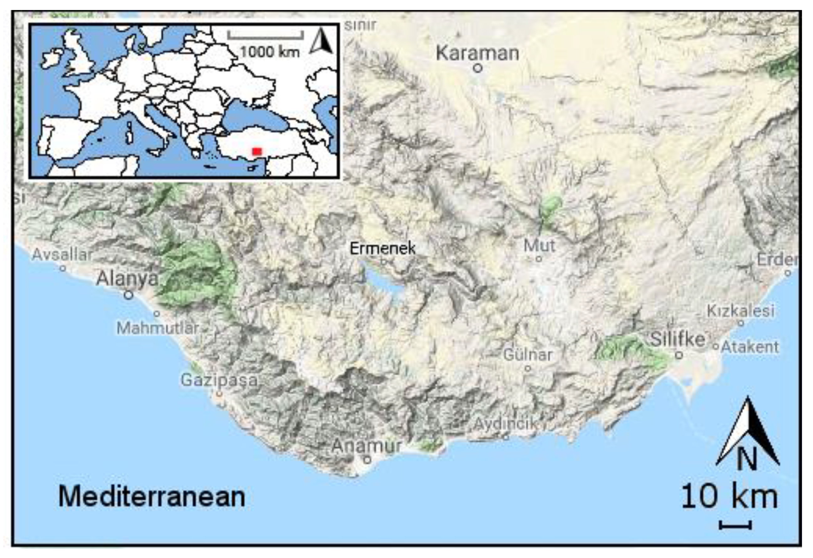
In the study, data measured in the Ermenek Dam, which is within the boundaries of the Ermenek District of Karaman Province, were used. The district is located between 36°58′ N and 32°53′ E. The average height of the district from sea level is 1250 m. The town of Ermenek contains many river sources, plateaus, promenades, as well as sources of historical and natural beauty. The Ermenek River, one of the crucial streams in the region, collects almost all waters of the region. Ermenek District, with an area of 122,297 ha, covers 13.86% of Karaman and 0.16% of Turkey. Of the total area, 21% of the district is farmland, 10% is meadow-pasture, and 38% is forest area [23,24,25,26].
Data used in the research belong to the Ermenek Dam, which was opened in 2009 with an installed capacity of 308.88 MW and an annual electricity generation capacity of 1187 GWh. The body of the dam is a concrete arch, and the crest length is 123 m. The filling volume is 305,000 m3, and the storage volume is 4582 billion m3 [27].
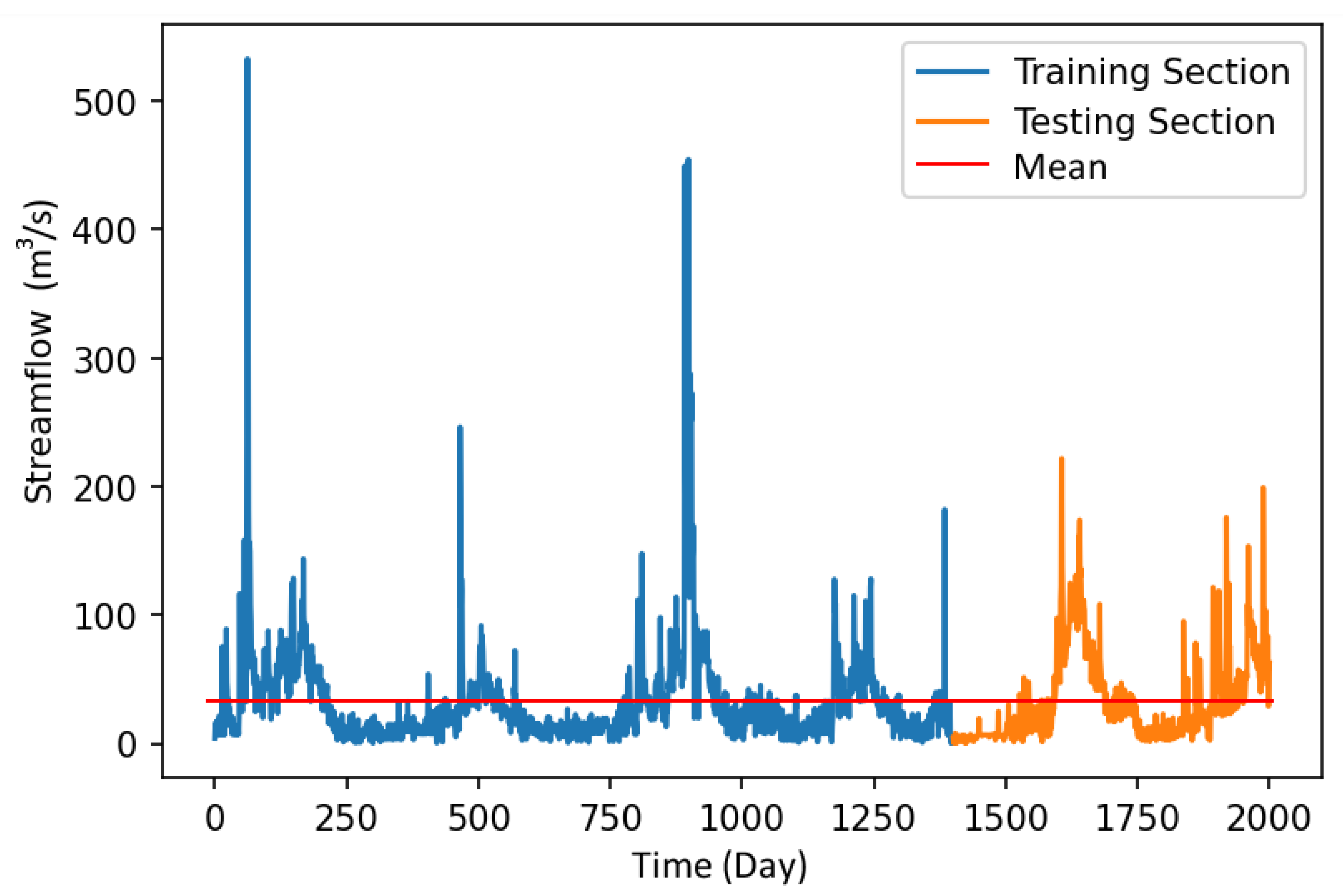
To simulate streamflow to the Ermenek Dam (Figure 1), daily mean inflow data are used during the 2012–2018 period. The basic characteristics of the data are provided in Table 1, and the time-series plots are displayed in Figure 2.
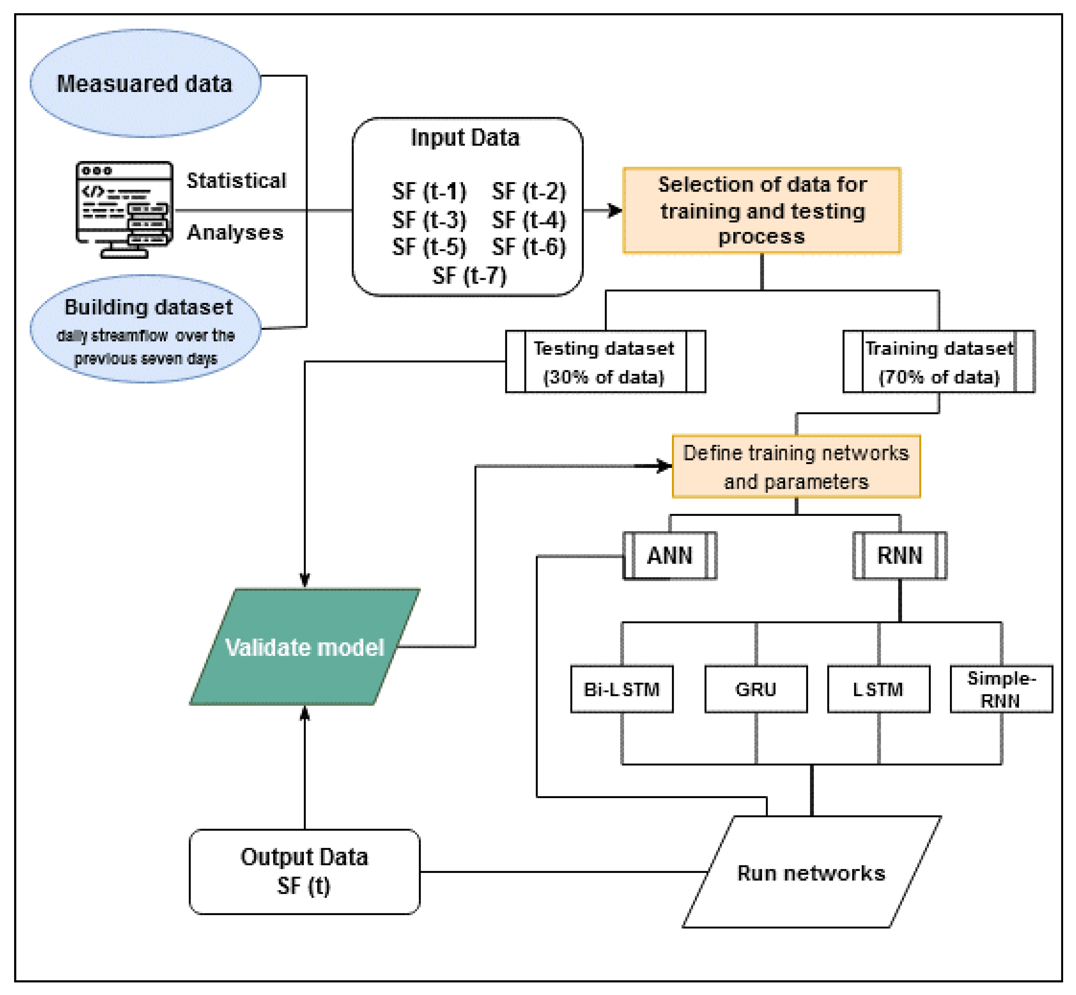
For modeling, ANN methods and four different RNN deep-network methods were employed. In total, 70% and 30% of the data were used in training and testing stages, respectively, as indicated in Figure 2. Besides this, several delayed daily mean streamflow are used as input data. For this purpose, the correlation between the time series of streamflows with its delays is obtained, and seven delays (SFt-1, SFt-2, SFt-3, SFt-4, SFt-5, SFt-6, and SFt-7) are selected as inputs due to high correlation (Figure 3). The correlation coefficients are found to vary between 0.63 and 0.85 in seven-day lag conditions. Similar studies [7,8] have also used seven delays in flow time series as inputs.
2.2. Artificial Neural Network (ANN)
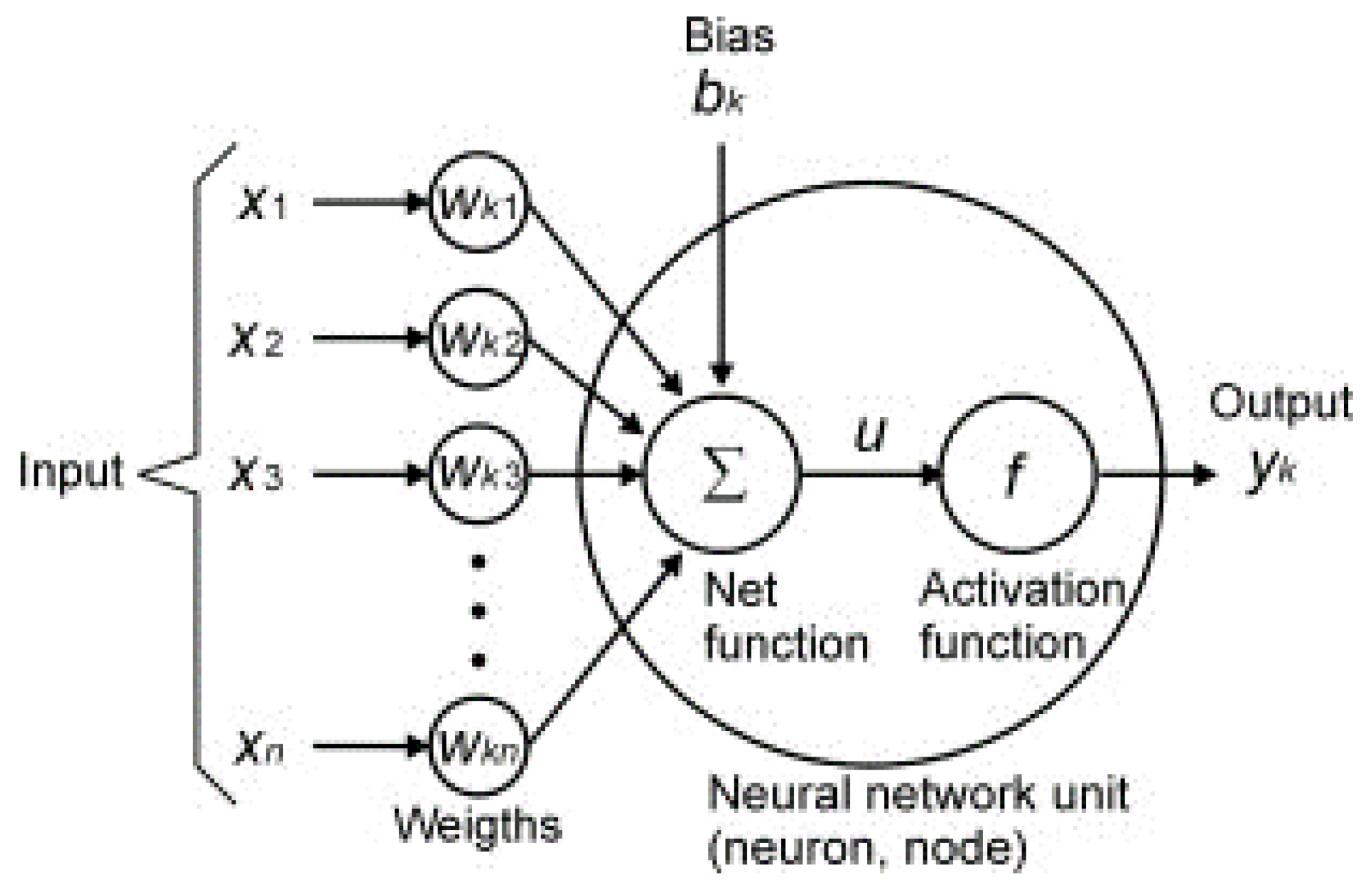
An ANN is a distributed knowledge treatment system in which performance essentials are alike to the human brain, and is based on a simulated biological neural network [28]. Each neural network has three layers, namely, input, hidden, and output. The input layer is a layer for providing data provided as inputs to the network. The output layer contains values predicted by the network. The hidden layer is the data analysis location. Usually, the number of selected neurons of the layers is obtained by trial and error. The general architecture of the ANN is displayed in Figure 4, where X (x1, x2, ..., xn) = inputs vector, W = connecting weights to the next layer, bk = bias, and yk is the ANN final output. The activation function converts input signals into output signals.
In Figure 4, N inputs are given from x1 to xn to the counterpart weights Wk1 to Wkn. Initially, the weights are multiplied by their inputs, and then they are summed with the amount of bias to obtain u (Equation (1)):
u = ∑w × x + b
Then, the activation function is adapted on u, i.e., f (u); ultimately, the final output value is obtained as of the neuron. The most popular activation functions are Sigmoid, ReLU, and Softmax. In this study, feed-forward neural networks were used.
2.3. Recurrent Neural Networks (RNN)
Deep-learning algorithms are a sample of machine-learning algorithms where the purpose is to discover multiple levels of representation of input data. Developed in the 1980s, multilayer RNNs are among the most commonly used models for deep learning [30]. These types of networks have a memory that records the information they have seen so far, and many types exist. Moreover, RNNs are powerful models for sequential data (time series) [31], and they use the previous output to predict the next output. In this case, the networks themselves have repetitive loops. These loops, which are in the hidden neurons, allow the storing of previous input information for a while so that the system can predict future outputs. The hidden layer output is retransmitted t times to the hidden layer. The output of a recursive neuron is only sent to the next layer when the number of iterations is completed. In this case, the output is more comprehensive, and the previous information is kept for longer. Finally, the errors are returned backward to update the weights. In this study, four available RNN architectures are used. In order to improve the readability of this study, a research flow chart is given in Figure 5.
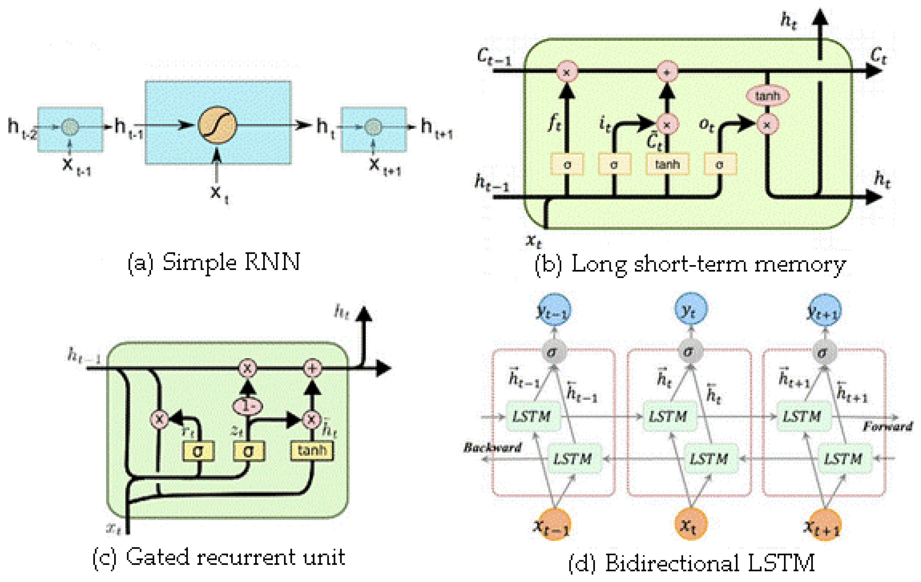
2.3.1. Simple Recurrent Neural Network (Simple RNN)
A simple RNN is essentially a collection of common neural networks arranged together, each of them transmitting a message to another. In other words, these networks have a memory that stores knowledge about the data seen, but their memory is short term and cannot maintain long-term time series [32]. Figure 6a displays a simple RNN. A simple recurrent network has only one internal memory——which is computed from Equation (2):
where g() denotes an activation function, U and W are flexible weight matrices of the h layer, b is a bias, and X is an input vector [19].
2.3.2. Long Short-Term Memory (LSTM)
LSTM is a kind of model or structure for sequential data developed by [33] for the advancement of RNN. It uses a special combination of hidden units, elementwise products, and sums between units to implement gates that control “memory cells.” These cells are designed to retain information without modification for long periods [34]. The greatest feature of LSTM is in its capability to learn long-term dependency, which is not possible with simple RNNs. To predict the next step, the weight values on the network have to be updated, which requires the maintenance of information from the initial steps. A simple RNN can only learn a limited number of short-term relationships and it cannot learn long-term series. However, LSTM can learn these long-term dependencies properly, and LSTM has three gates: input, forget, and output (Figure 6b). The forget gate is embedded to indicate how much the previous memory remembers and how much it has forgotten. For LSTM, the hidden state is computed as follows:
where , , and are the input, forget, and output gates at time t, respectively; , , , and are weights that map the hidden layer input to the three gates of input, forget, and output while , , , and weights matrices map the hidden layer output to gates; , , , and are vectors. Moreover, and are the outcome of the cell and the outcome of the layer, respectively [35].
2.3.3. Gated Recurrent Unit (GRU)
GRU is a simple type of LSTM suggested by Cho et al. [36]. The variance with LSTM is that GRU merges the input and forget gates and converts them with an update gate. Therefore, GRU has fewer parameters than LSTM which makes training easier. For GRU, the output value of is computed as follows:
where r is a reset gate, and z denotes an update gate. The reset gate indicates how the new input can be combined with earlier memory. The update gate also indicates how much previous memory is kept. If the update gate is 1, the previous memory is fully preserved, and if it is 0, the previous memory is completely forgotten. There is a forget gate in the LSTM that automatically determines how much of the previous memory is maintained whereas, in GRU, all previous memories are maintained or completely forgotten (Figure 6c). For some problems, GRUs can provide a performance comparable with LSTMs, but with a lower memory requirement [34,36].
2.3.4. Bidirectional LSTM (Bi-LSTM)
In fact, instead of one direction, the network is processed on two sides: backward and forward with two separate hidden layers. Graves and Schmidhuber [37] demonstrated that bidirectional networks responded better than unidirectional networks in cases such as phonemic clustering. The structure of a bidirectional network is displayed in Figure 6d. Given this figure, these networks have a structure with a forward and backward LSTM layer. The forward layer output order, , is repeatedly computed via inputs in a positive order from time T − n to time T − 1, while the backward layer outcome order, , is computed using the inverted inputs from time T − n to T − 1 [35]. The output of both forward and backward layers is computed in a similar manner to the unidirectional LSTM. In the Bi-LSTM layer, is computed from Equation (13):
where σ is a function used to merge two and outputs [35].
In all networks, the dropout function is used among layers, which is a technique to prevent network overfitting. This means that learning on different architectures occurs with a variety of neurons. Figure 7a,b illustrate networks before and after dropout, respectively.
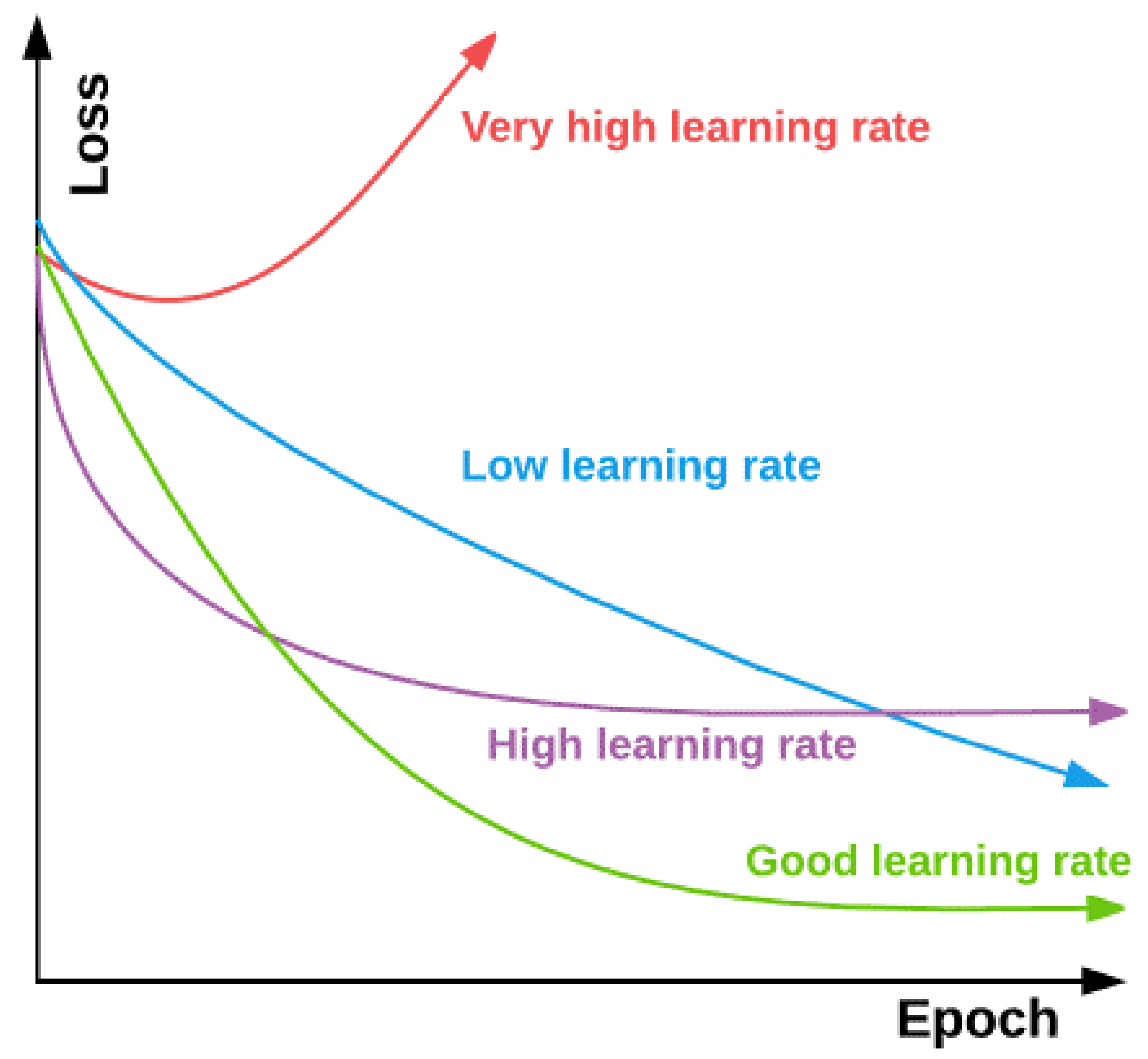
The learning rate is one of the hyperparameters necessary to find the optimal value and usually takes values between 1 and 1 × 10⁻⁷. In fact, the learning rate expresses the size of the move steps by the network. Figure 8 compares the changes in the loss function versus the epoch based on the learning rate. Working with a low learning rate, it takes a long time to find the best solution. Besides, if the learning rate is too high, it rejects the optimal mode. Since a high learning rate is advantageous in early iterations, and a low one is advantageous in later iterations, a learning rate that slows down as the algorithm progresses is preferred [39].
2.4. Open-Source Software and Codes
This research relies heavily on open-source software. Python 3.6 is used as a programming language. The libraries are used for preprocessing the data and for data management, including Pandas, Numpy, and Scikit-Learn. Deep-learning frameworks employed are TensorFlow and Keras. Different codes are used for each RNN and ANN. All figures are created using Matplotlib.
2.5. Evaluation Criteria
In order to evaluate the models, correlation coefficients (CC), Nash–Sutcliff coefficient (NS), root mean square error (RMSE), and mean absolute error (MAE) are used, as presented in Equations (14) to (17), respectively.
where is the observation parameter with a mean denoted by ; is the prediction parameter with a mean denoted by ; N is a number of instances. The more the two first criteria are closer to 1 and the next three values are closer to 0 show the better performance of the model. According to Chiew et al. [41], if NS > 0.90, the simulation is very acceptable; if 0.60 < NS < 0.90, the simulation is acceptable; and if NS < 0.60 as in this case, simulation is unacceptable.
3. Results and Discussion
In this research, daily streamflow to the Ermenek Dam reservoir in Turkey was simulated using various deep-learning models. In this section, the historical observation streamflow data are compared with the computed streamflow from artificial neural networks and RNN, such as Bi-LSTM, GRU, LSTM, and simple RNN using seven lag days. A network attempts to predict outcomes as accurately as possible. The value of this precision in the network is obtained by the cost function, which tries to penalize the network when it fails. The optimal output is the one with the lowest cost. In this study, for the applied networks of MSE, the cost function is used. A repetition step in training generally works with a division of training data named a batch size. The number of samples for each batch is a hyperparameter, which is normally obtained by trial and error. In this study, the value of this parameter in all models is 512 in the best mode. In each repetition step, the cost function is computed as the mean MSE of these 512 samples of observed and predicted streamflow. The number of iteration steps for neural networks is named an epoch; in each epoch, the streamflow time series is simulated by the network once. Like other networks, neurons or network layers can be selected arbitrarily in recurrent networks. For the purpose of the comparison of models with each other, the structures of all recurrent network models are created identically. In each network, a double hidden layer is used so that there are 200 units in the first layer and 150 units of the neuron in the second layer. The last layer output of the network at the final time step is linked to a dense layer with a single output neuron. Between the layers, a dropout equal to 10% is used. The structure of the neural network is also used in two hidden layers. The first and second layers have 200 and 150 neurons, respectively. In all networks, the ReLU activation function is applied for the hidden layer. The main advantage of using ReLU is that, for all inputs greater than 0, there is a fixed derivative. This constant derivative speeds up network learning. Each method is run with epoch numbers of 100, 200, and 500. Results of different methods based on the evaluation criteria and their running times are presented in Table 2 (Computations are performed using a Pentium B960, 2.20 GHz laptop computer with Windows 8 and 4 GB RAM.). Among the methods, ANN is the fastest; among RNN methods, the speed sequence is as follows: simple RNN, GRU, LSTM, and Bi-LSTM.
Different models are run with different iterations. As seen in Table 2, the number of epochs as one of the influential parameters plays a basic role; so in fewer iterations, the accuracy of the model is low, and the error is greater. By increasing the number of iterations, the model gradually converges so that there is not a significant difference between the results of 300 and 500 epochs. For this reason, it is decided that a maximum of 500 epochs is sufficient. Another parameter that influences the accuracy of the models is the number of neurons in the hidden layers. If it is low, the model will not be able to simulate correctly, and if it is too high, there is a risk of overfitting. This problem is solved by using the dropout method, which in fact deactivates several neurons. The values of the learning rate (LR) and decay are also presented in Table 2. Decay occurs due to how much the learning rate is reduced in each step. As seen in Table 2, five different evaluation criteria are used to compare five different prediction methods. Each method has the best result with 300 or 500 epochs. The performance of the testing stage is generally 1–5% lower than that of the training stage. According to Table 2, among the methods used, the LSTM method performs best in 500 epochs with an accuracy of CC = 87% in the testing stage. This network has long-term memory, and its forget gate specifies how much previous memory is kept. The first step is the multiplication of input data in weights and then its summation with the bias, followed by output. In this step, the output is likely to be very different from the actual output. Therefore, errors are returned backward to update the weights and also biases.
Comparison of some metrics by all methods used in the study are given in Table 3. In this table, measured streamflow values (those set aside for the test and the whole streamflow data set) and values predicted by the methods can be compared. The GRU and LSTM models had the closest results to measured values in max, mean, and standard deviation (StDev) statistics in terms of similarity to the measured values. Simple RNN, ANN, and BLSTM methods gave the worst results, respectively.
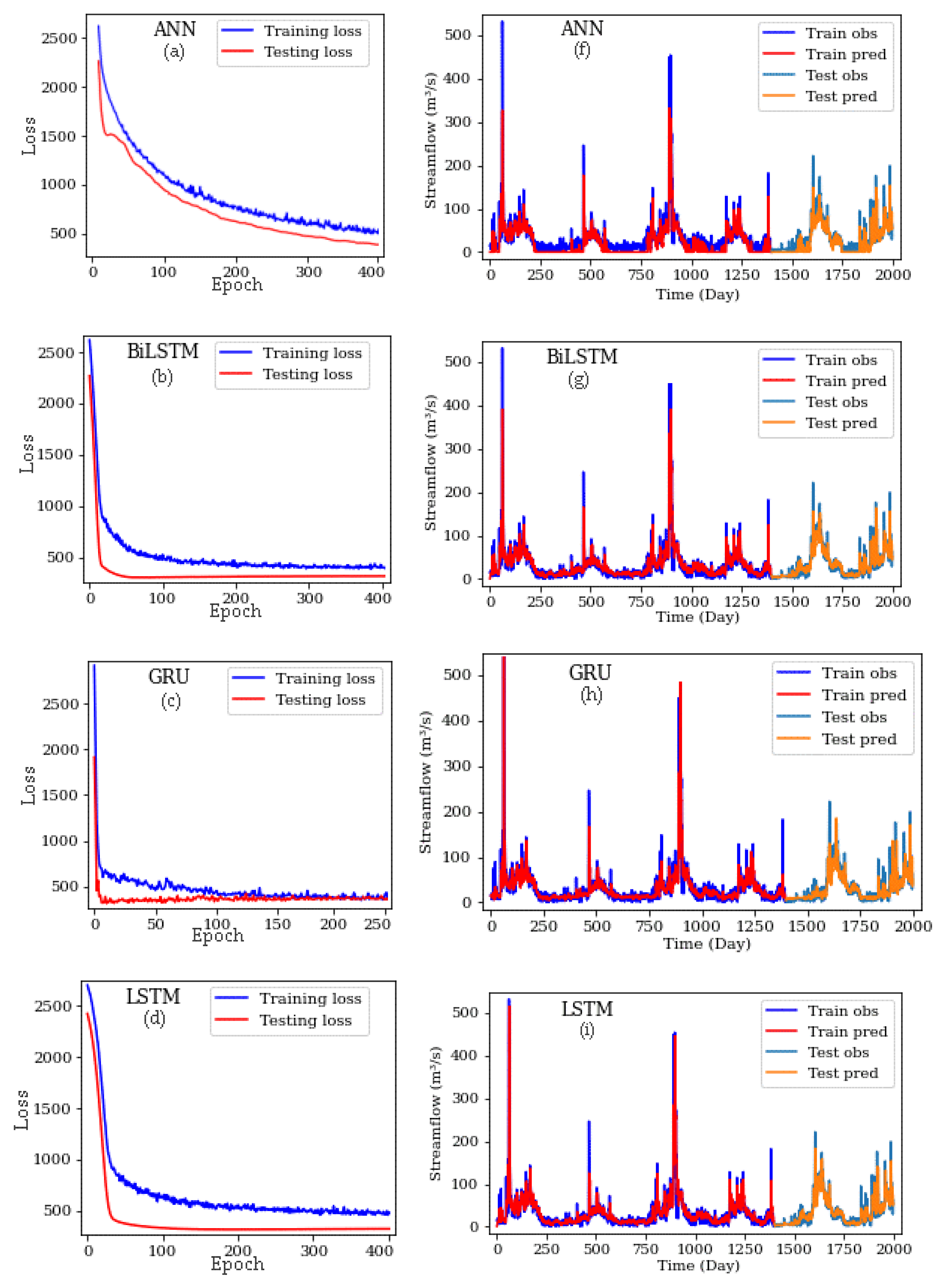
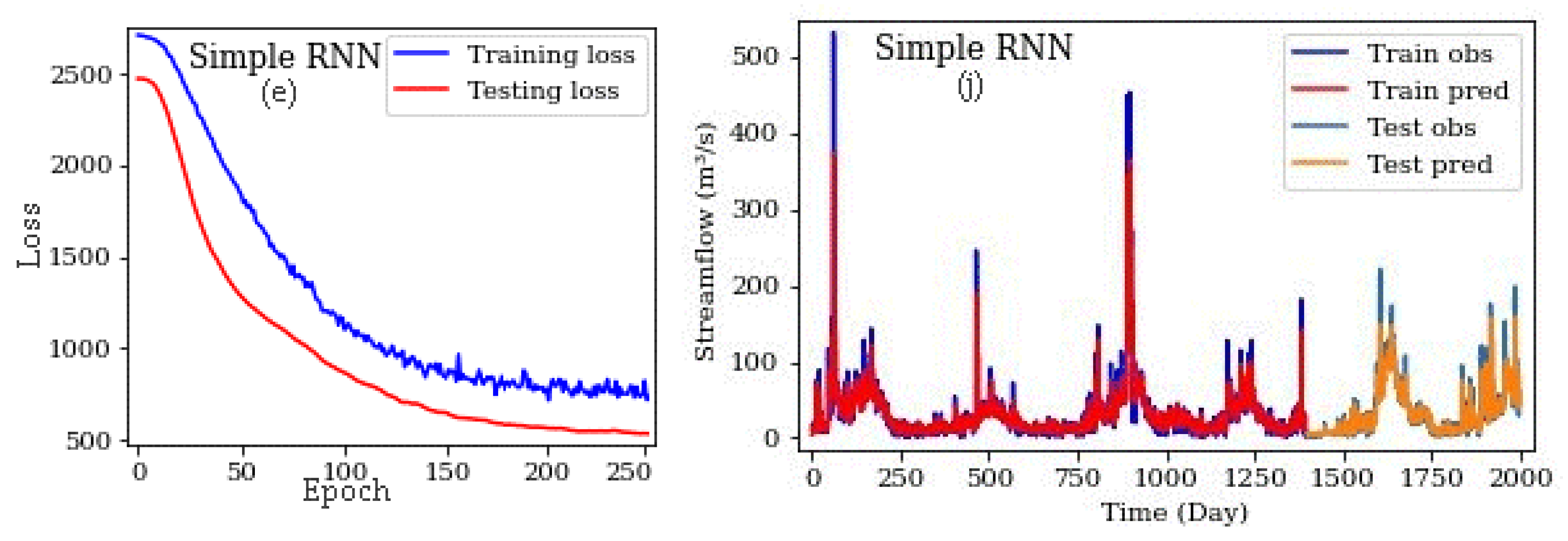
The loss function, observational streamflow values and predicted values for training and testing stages computed by various methods are displayed in Figure 9. When the loss function and time-series graphs are examined, the most successful methods are LSTM and GRU. The loss charts of testing and training stages of both methods overlap at the highest epoch value. According to the loss function graphs (Figure 9), with the reduction of the modeling error for the training stage, the error of the testing stage decreases, and the distance between the two graph lines reduces. Therefore, it can be said that the dropout function helps to prevent network overfitting. Besides, considering the changes in the loss function value versus epochs (and according to Figure 8) can ensure that the learning rate is selected correctly.
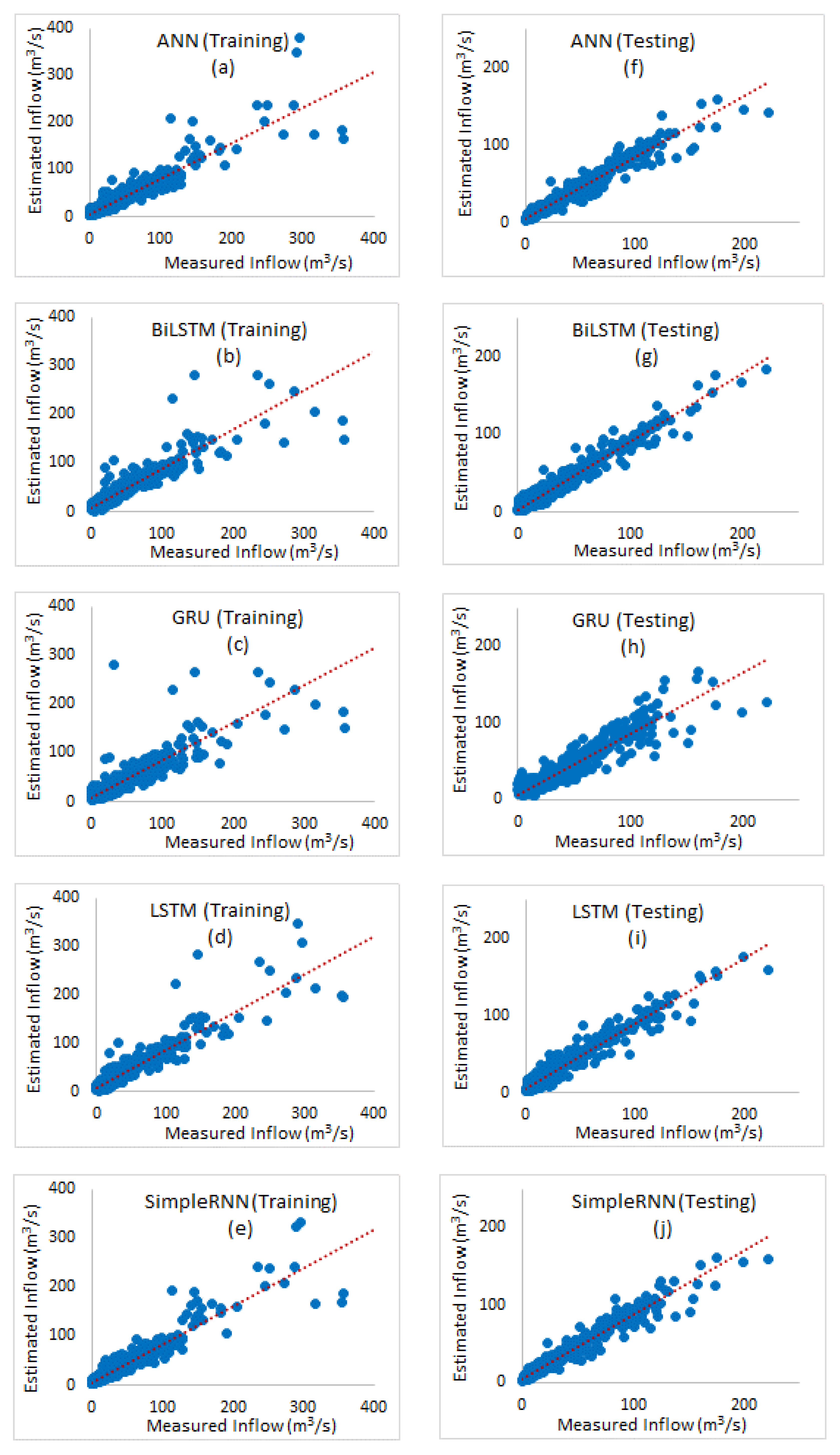
Figure 10 shows the scatter of observed values versus the predicted values for both training and testing stages. Regarding the streamflow graphs (Figure 9 and Figure 10), the networks yield poor results in peak periods and cannot simulate these periods well, except LSTM. One major reason of this is that streamflow abundance has very few high values, and the network cannot properly learn them. This happens even though the streamflow abundance has several low values, so the model can correctly and accurately be learned in the training stage. According to the data, the difference between the minimum and the maximum flow values is high, and the validity of these values is investigated during the study period based on precipitation in the region. In periods where peak streamflow is observed, the maximum rainfall is observed with a significant amount that indicates the correctness of peak flow values. However, among the methods applied, the LSTM network is better than other methods, and is able to simulate peak flow periods fairly. As noted above, the greatest feature of this network is its skill to learn long-term dependencies, and the forget gate makes the network keep or forget the desired amount of previous memory and thus helps to improve the modeling. The GRU method is similar to the LSTM method, and its results are close to those of LSTM. In contrast, the other methods failed to simulate peak flow values. The scatter plots in Figure 10 indicate a relatively small dispersion of observed and predicted data in training and testing stages compared to other methods. Kratzert et al. [19] used deep LSTM networks in similar research and demonstrated that these networks perform better than other networks and can be used in hydrological simulations as an application method.
4. Conclusions
In this paper, a novel approach to streamflow simulation based on recurrent neural networks is presented. For this purpose, 70% of the inflow data are trained to ANN and RNNs, including Bi-LSTM, LSTM, GRU, and simple RNN. Then, the 30% remaining data were predicted. For each of the networks, the double hidden layer was used. The number of neurons in the hidden layers, the learning rate, and the number of iterations have a basic role in modeling accuracy, the optimal values of which were obtained using trial and error. Using the dropout function in the network structure can well prevent network overfitting. To attain this purpose, all models were coded in Python programming software. The efficiency of the proposed approach is evaluated for the simulation of daily inflow to the Ermenek Dam reservoir in Turkey. Results of the study point to the better performance of recurrent networks (NS: 0.74, RMSE:17.92) compared to ANN (NS: 0.72, RMSE:18.71). Among different RNN architectures, the LSTM network performed the best and can estimate streamflow with fairly good accuracy (CC: 0.87), and it can be said that these networks can be used as an effective method of streamflow modeling and simulation.
Thermal power plants are not environmentally friendly and cause air pollution and global warming. Due to limited fossil resources in Turkey the importance of the hydroelectric power plant is increased. Considering the purpose of the reservoir construction, which is the production of the hydroelectric power or agricultural irrigation, the prediction of streamflow may help to increase efficiency and achieve the desired purpose. In this study, for the first time, deep learning methods are used to model inflows to the Ermenek Dam reservoir located in Turkey. Results of this study are consistent with those of studies by Nagesh Kumar et al. [5] and Zhang et al. [17] Given that water resource management is essential, it can be acknowledged that the use of these methods can help managers and officials of the Ermenek Dam in future planning. As a result, increasing the accuracy of the model can help researchers and experts to achieve this goal.
Author Contributions
Conceptualization, M.T.S., and H.A.; Data curation, M.S.C., and H.F.; Formal analysis, H.F. and S.S.; Funding acquisition, M.T.S., H.A. and S.S.; Investigation, M.T.S., H.A. K.-W.C. and S.S.; Methodology, M.T.S., H.A. and S.S.; Project administration, H.A.; Resources, M.T.S., K.-W.C. and H.A.; Software, H.F., M.T.S. and H.A.; Supervision, M.T.S, H.A. and S.S.; Validation, M.T.S, H.A. and S.S.; Visualization, H.F., M.S.C., H.A. and S.S.; Writing—original draft, H.F. M.T.S., H.A. and M.S.C.; Writing—review and editing, M.T.S. K.-W.C., H.A. and S.S. All authors have read and agreed to the published version of the manuscript.
Funding
This research received no external funding.
Conflicts of Interest
The authors declare no conflict of interest.
References
- Hamlet, A.F.; Lettenmaier, D.P. Columbia River Streamflow Forecasting Based on ENSO and PDO Climate Signals. J. Water Resour. Plan. Manag. 1999, 125, 333–341. [Google Scholar] [CrossRef]
- Ghumman, A.R.; Ghazaw, Y.M.; Sohail, A.R.; Watanabe, K. Runoff forecasting by artificial neural network and conventional model. Alex. Eng. J. 2011, 50, 345–350. [Google Scholar] [CrossRef] [Green Version]
- Bengio, Y. Learning Deep Architectures for AI by Yoshua Bengio; Now Publishers: Montréal, QC, Canada, 2009; Volume 2. [Google Scholar] [CrossRef]
- Elumalai, V.; Brindha, K.; Sithole, B.; Lakshmanan, E. Spatial interpolation methods and geostatistics for mapping groundwater contamination in a coastal area. Environ. Sci. Pollut. Res. 2017, 21, 11601–11617. [Google Scholar] [CrossRef] [PubMed]
- Kumar, D.N.; Raju, K.S.; Sathish, T. River Flow Forecasting using Recurrent Neural Networks. Water Resour. Manag. 2004, 18, 143–161. [Google Scholar] [CrossRef]
- Pan, T.-Y.; Wang, R.-Y.; Lai, J.-S. A deterministic linearized recurrent neural network for recognizing the transition of rainfall–runoff processes. Adv. Water Resour. 2007, 30, 1797–1814. [Google Scholar] [CrossRef]
- Firat, M. Comparison of Artificial Intelligence Techniques for river flow forecasting. Hydrol. Earth Syst. Sci. 2008, 12, 123–139. [Google Scholar] [CrossRef] [Green Version]
- Sattari, M.T.; Yurekli, K.; Pal, M. Performance evaluation of artificial neural network approaches in forecasting reservoir inflow. Appl. Math. Model. 2012, 36, 2649–2657. [Google Scholar] [CrossRef]
- Sattari, M.T.; Apaydin, H.; Ozturk, F. Flow estimations for the Sohu Stream using artificial neural networks. Envron. Earth Sci. 2011, 66, 2031–2045. [Google Scholar] [CrossRef]
- Chen, P.-A.; Chang, L.-C.; Chang, L.-C. Reinforced recurrent neural networks for multi-step-ahead flood forecasts. J. Hydrol. 2013, 497, 71–79. [Google Scholar] [CrossRef]
- Sattari, M.T.; Pal, M.; Apaydin, H.; Ozturk, F. M5 model tree application in daily river flow forecasting in Sohu Stream, Turkey. Water Resour. 2013, 40, 233–242. [Google Scholar] [CrossRef]
- Chang, L.-C.; Chen, P.-A.; Lu, Y.-R.; Huang, E.; Chang, K.-Y. Real-time multi-step-ahead water level forecasting by recurrent neural networks for urban flood control. J. Hydrol. 2014, 517, 836–846. [Google Scholar] [CrossRef]
- Liu, F.; Xu, F.; Yang, S. A Flood Forecasting Model Based on Deep Learning Algorithm via Integrating Stacked Autoencoders with BP Neural Network. In Proceedings of the 2017 IEEE Third International Conference on Multimedia Big Data (BigMM), Laguna Hills, CA, USA, 19–21 April 2017; pp. 58–61. [Google Scholar] [CrossRef]
- Esmaeilzadeh, B.; Sattari, M.T.; Samadianfard, S. Performance evaluation of ANNs and an M5 model tree in Sattarkhan Reservoir inflow prediction. ISH J. Hydraul. Eng. 2017, 11, 1–10. [Google Scholar] [CrossRef]
- Amnatsan, S.; Yoshikawa, S.; Kanae, S. Improved Forecasting of Extreme Monthly Reservoir Inflow Using an Analogue-Based Forecasting Method: A Case Study of the Sirikit Dam in Thailand. Water 2018, 10, 1614. [Google Scholar] [CrossRef] [Green Version]
- Chiang, Y.-M.; Hao, R.-N.; Zhang, J.-Q.; Lin, Y.-T.; Tsai, W.-P. Identifying the Sensitivity of Ensemble Streamflow Prediction by Artificial Intelligence. Water 2018, 10, 1341. [Google Scholar] [CrossRef] [Green Version]
- Zhang, D.; Peng, Q.; Lin, J.; Wang, D.; Liu, X.; Zhuang, J. Simulating Reservoir Operation Using a Recurrent Neural Network Algorithm. Water 2019, 11, 865. [Google Scholar] [CrossRef] [Green Version]
- Zhou, Y.; Guo, S.; Xu, C.-Y.; Chang, F.-J.; Yin, J. Improving the Reliability of Probabilistic Multi-Step-Ahead Flood Forecasting by Fusing Unscented Kalman Filter with Recurrent Neural Network. Water 2020, 12, 578. [Google Scholar] [CrossRef] [Green Version]
- Kratzert, F.; Klotz, D.; Brenner, C.; Schulz, K.; Herrnegger, M. Rainfall–runoff modelling using Long Short-Term Memory (LSTM) networks. Hydrol. Earth Syst. Sci. 2018, 22, 6005–6022. [Google Scholar] [CrossRef] [Green Version]
- Zhang, D.; Lin, J.; Peng, Q.; Wang, D.; Yang, T.; Sorooshian, S.; Liu, X.; Zhuang, J. Modeling and simulating of reservoir operation using the artificial neural network, support vector regression, deep learning algorithm. J. Hydrol. 2018, 565, 720–736. [Google Scholar] [CrossRef] [Green Version]
- Kao, I.-F.; Zhou, Y.; Chang, L.-C.; Chang, F.-J. Exploring a Long Short-Term Memory based Encoder-Decoder framework for multi-step-ahead flood forecasting. J. Hydrol. 2020, 583, 124631. [Google Scholar] [CrossRef]
- Zhou, J.; Peng, T.; Zhang, C.; Sun, N. Data Pre-Analysis and Ensemble of Various Artificial Neural Networks for Monthly Streamflow Forecasting. Water 2018, 10, 628. [Google Scholar] [CrossRef] [Green Version]
- Anonymous. Karaman Province Government, Statistics of Agricultural Section. Available online: https://karaman.tarimorman.gov.tr/ (accessed on 15 March 2019). (In Turkish)
- Anonymous. Mevlana Development Agency, Ermenek District Report 2014. Available online: http://www.mevka.org.tr/Yukleme/Uploads/DsyHvaoSM719201734625PM.pdf (accessed on 15 March 2019). (In Turkish).
- DSI. Available online: http://www.dsi.gov.tr/dsi-resmi-istatistikler (accessed on 15 March 2019). (In Turkish)
- Ghaffarinasab, N.; Ghazanfari, M.; Teimoury, E. Hub-and-spoke logistics network design for third party logistics service providers. Int. J. Manag. Sci. Eng. Manag. 2015, 11, 1–13. [Google Scholar] [CrossRef]
- Anonymous. Ermenek Dam and Hydroelectricity Facility Catalogue; The Ministry of Energy and Natural Resources: Karaman, Turkey, 2019. (In Turkish)
- Gao, C.; Gemmer, M.; Zeng, X.; Liu, B.; Su, B.; Wen, Y. Projected streamflow in the Huaihe River Basin (2010–2100) using artificial neural network. Stoch. Environ. Res. Risk Assess. 2010, 24, 685–697. [Google Scholar] [CrossRef]
- Li, F.; Johnson, J.; Yeung, S. Cource Notes. Lecture 4—1 April 12, 2018. Available online: http://cs231n.stanford.edu/slides/2018/cs231n_2018_lecture04.pdf (accessed on 20 May 2019).
- Schmidhuber, J. System Modeling and Optimization. The Technical University of Munich (TUM) Habilitation Thesis. 1993. Available online: http://people.idsia.ch/~juergen/onlinepub.html (accessed on 20 May 2019).
- Graves, A.; Mohamed, A.-R.; Hinton, G.; Graves, A. Speech recognition with deep recurrent neural networks. In Proceedings of the IEEE International Conference on Acoustics, Speech and Signal Processing, Vancouver, BC, Canada, 26–31 May 2013; pp. 6645–6649. [Google Scholar] [CrossRef] [Green Version]
- Bengio, Y.; Simard, P.; Frasconi, P. Learning long-term dependencies with gradient descent is difficult. IEEE Trans. Neural Netw. 1994, 5, 157–166. [Google Scholar] [CrossRef] [PubMed]
- Hochreiter, S.; Schmidhuber, J. Long Short-Term Memory. Neural Comput. 1997, 9, 1735–1780. [Google Scholar] [CrossRef] [PubMed]
- Witten, I.; Frank, E.; Hall, M.; Pal, C. Data Mining. In Practical Machine Learning Tools and Techniques, 4th ed.; Elsevier: Amsterdam, The Netherlands, 2016; p. 654. ISBN 9780128042915. [Google Scholar]
- Cui, Z.; Member, S.; Ke, R.; Member, S.; Wang, Y. Deep Stacked Bidirectional and Unidirectional LSTM Recurrent Neural Network for Network-wide Traffic Speed Prediction. In Proceedings of the UrbComp 2017: The 6th International Workshop on Urban Computing, Halifax, NS, Canada, 14 August 2017; 2017; pp. 1–12. [Google Scholar]
- Cho, K.; Van Merrienboer, B.; Bahdanau, D.; Bengio, Y. On the Properties of Neural Machine Translation: Encoder–Decoder Approaches. In Proceedings of the SSST-8, Eighth Workshop on Syntax, Semantics and Structure in Statistical Translation, Doha, Qatar, 7 October 2014; pp. 103–111. [Google Scholar]
- Graves, A.; Schmidhuber, J. Framewise phoneme classification with bidirectional LSTM and other neural network architectures. Neural Netw. 2005, 18, 602–610. [Google Scholar] [CrossRef] [PubMed]
- The Effect of Dropout on the Network Structure. Available online: https://blog.faradars.org/ (accessed on 20 May 2019).
- Ashcroft, M. Advanced Machine Learning. Available online: https://www.futurelearn.com/courses/advanced-machine-learning/0/steps/49552 (accessed on 20 May 2019).
- Train/Val Accuracy. Available online: http://cs231n.github.io/neural-networks-3/#accuracy (accessed on 20 May 2019).
- Chiew, F.; Stewardson, M.J.; McMahon, T. Comparison of six rainfall-runoff modelling approaches. J. Hydrol. 1993, 147, 1–36. [Google Scholar] [CrossRef]
Figure 1.
Location of the study area.

Figure 2.
Streamflow time series.

Figure 3.
Correlation plot between streamflow and its delays.

Figure 4.
General structure of a neural network [29].
Figure 4.
General structure of a neural network [29].

Figure 5.
The flow chart of the modelling processes. *SF: Streamflow, t: delayed day, ANN: Artificial neural network, RNN: Recurrent neural network, Bi-LSTM: Bidirectional long short-term memory, GRU: Gated recurrent unit, LSTM: Long short-term memory, simple RNN: simple recurrent neural networks.
Figure 5.
The flow chart of the modelling processes. *SF: Streamflow, t: delayed day, ANN: Artificial neural network, RNN: Recurrent neural network, Bi-LSTM: Bidirectional long short-term memory, GRU: Gated recurrent unit, LSTM: Long short-term memory, simple RNN: simple recurrent neural networks.

Figure 6.
The general structure of recurrent neural network models. (a) Simple RNN, (b) LSTM, (c) GRU, and (d) Bi-LSTM models [19].
Figure 6.
The general structure of recurrent neural network models. (a) Simple RNN, (b) LSTM, (c) GRU, and (d) Bi-LSTM models [19].

Figure 7.
Structure of networks (a) before and (b) after applying dropout [38].
Figure 7.
Structure of networks (a) before and (b) after applying dropout [38].

Figure 8.
Changes in the loss function vs. the epoch by the learning rate [40].
Figure 8.
Changes in the loss function vs. the epoch by the learning rate [40].

Figure 9.
Loss function plots (a–e), observed and computed time series (f–j) for different methods in training and testing stages.
Figure 9.
Loss function plots (a–e), observed and computed time series (f–j) for different methods in training and testing stages.


Figure 10.
Scatter plots of inflow for different methods in training (a–e) and testing (f–j) stages.
Figure 10.
Scatter plots of inflow for different methods in training (a–e) and testing (f–j) stages.


Table 1.
Statistical characteristics of daily streamflow and rainfall.
| Variable | Min | Max | Mean | Std. Deviation |
|---|---|---|---|---|
| Streamflow (m3/s) | 0.04 | 532.76 | 33.21 | 39.32 |
| Rainfall (mm/day) | 0.0 | 52.00 | 1.40 | 4.57 |
Table 2.
Results of different models *.
| Method | Lr | Decay | Epoch | Run Time | CC | NS | RMSE | MAE | ||||
|---|---|---|---|---|---|---|---|---|---|---|---|---|
| Train | Test | Train | Test | Train | Test | Train | Test | |||||
| ANN | 1 × 10⁻³ | 1 × 10⁻² | 100 | 0:00:09 | 0.8 | 0.8 | 0.24 | 0.1 | 35.73 | 33.4 | 23.37 | 24.13 |
| 1 × 10⁻³ | 1 × 10⁻² | 300 | 0:00:29 | 0.82 | 0.82 | 0.43 | 0.36 | 30.91 | 28.86 | 19.56 | 19.65 | |
| 1 × 10⁻³ | 1 × 10⁻² | 500 | 0:00:51 | 0.86 | 0.85 | 0.73 | 0.72 | 21.11 | 18.71 | 10.51 | 10.35 | |
| Bi-LSTM | 1 × 10⁻⁴ | 1 × 10⁻³ | 100 | 0:02:45 | 0.83 | 0.83 | 0.64 | 0.56 | 33.7 | 29.19 | 21.24 | 20.81 |
| 1 × 10⁻⁴ | 1 × 10⁻² | 300 | 0:07:29 | 0.88 | 0.84 | 0.68 | 0.61 | 24.65 | 23.43 | 15.35 | 15.31 | |
| 1 × 10⁻⁴ | 1 × 10⁻² | 500 | 0:10:37 | 0.88 | 0.86 | 0.78 | 0.73 | 19.11 | 18.2 | 9.52 | 10.1 | |
| GRU | 1 × 10⁻⁴ | 1 × 10⁻² | 100 | 0:00:47 | 0.84 | 0.8 | 0.41 | 0.36 | 31.33 | 28.16 | 20.32 | 19.92 |
| 1 × 10⁻² | 1 × 10⁻² | 300 | 00:02.0 | 0.9 | 0.85 | 0.82 | 0.72 | 17.55 | 18.7 | 8.93 | 10.63 | |
| 1 × 10⁻⁴ | 1 × 10⁻³ | 500 | 00:03.1 | 0.9 | 0.85 | 0.77 | 0.67 | 19.58 | 20.12 | 11.67 | 12.46 | |
| LSTM | 1 × 10⁻⁴ | 1 × 10⁻³ | 100 | 0:00:53 | 0.85 | 0.81 | 0.5 | 0.41 | 26.98 | 28.89 | 18.53 | 18.78 |
| 1 × 10⁻⁴ | 1 × 10⁻³ | 300 | 0:02:17 | 0.89 | 0.84 | 0.76 | 0.64 | 20.1 | 21.16 | 12.15 | 13.15 | |
| 1 × 10⁻⁴ | 1 × 10⁻² | 500 | 0:03:37 | 0.87 | 0.87 | 0.74 | 0.74 | 20.75 | 17.92 | 10.22 | 9.98 | |
| Simple RNN | 1 × 10⁻⁴ | 1 × 10⁻³ | 100 | 0:00:30 | 0.8 | 0.83 | 0.36 | 0.31 | 32.63 | 29.25 | 21.74 | 21.21 |
| 1 × 10⁻⁴ | 1 × 10⁻³ | 300 | 0:01:09 | 0.85 | 0.86 | 0.71 | 0.71 | 21.94 | 18.31 | 10.71 | 10.11 | |
| 1 × 10⁻⁴ | 1 × 10⁻³ | 500 | 0:01:46 | 0.87 | 0.85 | 0.69 | 0.65 | 20.81 | 21.16 | 13.4 | 14.35 | |
* Bold indicates the best results.
Table 3.
Comparison of estimated values with observed values for all methods.
| Prediction Methods | Observed | |||||||
|---|---|---|---|---|---|---|---|---|
| Statistic | ANN | Bi-LSTM | GRU | LSTM | Simple RNN | Train Data | Test Data | All Data |
| Min (m3/s) | 2.40 | 2.16 | 4.74 | 1.73 | 1.76 | 0.09 | 0.04 | 0.04 |
| Max (m3/s) | 158.45 | 182.93 | 167.07 | 175.63 | 160.69 | 532.76 | 221.64 | 532.76 |
| Mean (m3/s) | 32.05 | 34.57 | 34.14 | 33.93 | 32.67 | 32.42 | 34.99 | 33.21 |
| Stdev (m3/s) | 28.8 | 31.3 | 29.7 | 30.6 | 30.2 | 40.9 | 35.2 | 39.3 |
| N. of instances | 600 | 600 | 600 | 600 | 600 | 1400 | 600 | 2000 |
© 2020 by the authors. Licensee MDPI, Basel, Switzerland. This article is an open access article distributed under the terms and conditions of the Creative Commons Attribution (CC BY) license (http://creativecommons.org/licenses/by/4.0/).
Share and Cite
MDPI and ACS Style
Apaydin, H.; Feizi, H.; Sattari, M.T.; Colak, M.S.; Shamshirband, S.; Chau, K.-W. Comparative Analysis of Recurrent Neural Network Architectures for Reservoir Inflow Forecasting. Water 2020, 12, 1500. https://doi.org/10.3390/w12051500
AMA Style
Apaydin H, Feizi H, Sattari MT, Colak MS, Shamshirband S, Chau K-W. Comparative Analysis of Recurrent Neural Network Architectures for Reservoir Inflow Forecasting. Water. 2020; 12(5):1500. https://doi.org/10.3390/w12051500
Chicago/Turabian StyleApaydin, Halit, Hajar Feizi, Mohammad Taghi Sattari, Muslume Sevba Colak, Shahaboddin Shamshirband, and Kwok-Wing Chau. 2020. "Comparative Analysis of Recurrent Neural Network Architectures for Reservoir Inflow Forecasting" Water 12, no. 5: 1500. https://doi.org/10.3390/w12051500
Note that from the first issue of 2016, this journal uses article numbers instead of page numbers. See further details here.