Spatiotemporal Water Yield Variations and Influencing Factors in the Lhasa River Basin, Tibetan Plateau

Abstract

Understanding the spatiotemporal characteristics of water yield and its influencing factors is important for water resources management. In this study, we used the seasonal water yield model (SWYM) to assess the spatiotemporal water yield changes of the Lhasa River Basin from 1990 to 2015, and analyzed its influencing factors by focusing on precipitation, land cover, and normalized difference vegetation index (NDVI) change. We first examined the model through Morris screening sensitivity analysis and validated it with the observed flow data. Spatiotemporal variation of three indices of water yield, baseflow, quick flow, and local recharge were then assessed. Results showed that from 1990 to 2015, the baseflow, local recharge, and quick flow decreased by 67.03%, 80.21%, and 37.03%, respectively. The spatial pattern of water yield remained mostly unchanged. According to the contribution analysis, precipitation and NDVI change were the main factors affecting water yield in the Lhasa River Basin, while land cover change began to exert greater influence after 2010. A combination of climate change and human activities therefore drive water yield change, especially through vegetation change. Water resources management strategies should thus take into account the combination of rapidly changing climate and human activities.

1. Introduction

Among the many ecosystem services that influence human wellbeing, water yield is of great importance as many agricultural, industrial, and domestic activities depend on it [1,2,3]. On one hand, the total amount of water yield influences or restricts the way in which people use water resources [4]. Additionally, the spatiotemporal variation in water yield is also important, and often leads to the challenge of how to allocate water resources between different seasons, and between upstream and downstream areas [2,5]. For arid and semi-arid regions, especially where the climate is highly seasonal, the baseflow that is slowly released by upstream areas due to the interception of vegetation or soil during the rainy season is highly valuable for downstream residents [6,7]. However, the quick flow that is soon released after heavy rainfalls also needs to be quantified since it directly contributes to flood and has substantial impact on soil erosion. Therefore, understanding the spatiotemporal variation in water yield including the baseflow, local recharge, and quick flow as well as their driving factors is critical for developing appropriate water resources management strategies [3,8,9,10].

Many studies have simulated and quantified water yield services as well as their influencing factors over different temporal and spatial scales using different models and methods. Zomlot et al. [10] assessed long-term average recharge and baseflow using a spatially-distributed water balance model WetSpass, and then analyzed the controlling factors using correlation analysis method. Ahiablame et al. [9] analyzed the influence of climate variability and agricultural land use change on annual baseflow, which was estimated through the Web-based Hydrograph Analysis Tool (WHAT). Jiang et al. [11] assessed changes in multiple ecosystem services in the Three-River Headwaters Region using the annual water yield model in InVEST (Integrated Valuation of Environmental Services and Tradeoffs), showing that the increase in precipitation significantly enhanced the water yield and soil erosion. Wang et al. [12] assessed the impact of land use and land cover change on streamflow based on the SWAT (Soil and Water Assessment Tool), and found that streamflow decreased on agricultural land, but increased in forest areas.

Although there are already many well developed hydrology models such as SWAT and VIC (Variable Infiltration Capacity) [13,14], there is still a huge need for hydrology models that can provide quick and spatially explicit assessment on seasonal water yield to better guide land and water resources management. As one of the most widely used ecosystem service assessment tools, InVEST first released the seasonal water yield model (SWYM) as a module in its 3.3.1 version in 2016 [6]. Unlike its previous annual water yield model, SWYM computes spatial indices that quantify the relative contribution of a parcel of land to the generation of both baseflow and quick flow [6]. It can also be easily used to explore the effects of climate and/or land use change on water yield [15]. With its simple interface, reduced data needs, and multiple-scenario setting function, SWYM has huge potential in understanding water resources and informing land management practices. However, so far, it has only been used in a handful of studies [15,16]. SWYM also lacks empirical validation and sensitivity analysis compared to the annual water yield model, which has been widely used and sufficiently validated in many areas [17,18,19].

Climate change and human activities are the two main driving factors influencing ecosystems, and their effects are usually intertwined [20]. The Tibetan Plateau is one of the most sensitive areas to global climate change, with a significant temperature rise of 0.3 °C per decade over 50 years [21,22], and the precipitation fluctuates greatly in some areas [23,24]. Studies have shown that climate change has significantly affected the grassland quality [20,25,26], which is the main vegetation type in the Tibetan Plateau. Located at the south-eastern part of the Tibetan Plateau, the Lhasa River Basin is the social and economic center of the Tibet Autonomous Region. How water yield changes spatiotemporally and how to better manage water resources under the combined influence of climate change and rapid socioeconomic developments have become an increasingly urgent challenge to the Lhasa River Basin and many other areas in the world.

In this paper, we used the SWYM to assess the spatiotemporal water yield changes of China’s Lhasa River Basin between 1990 and 2015, and analyzed its influencing factors. Specifically, we aimed to: (1) analyze the sensitivity of SWYM inputs and validate the model with observed data; (2) assess the spatiotemporal variation in the baseflow, local recharge, and quick flow from 1990 to 2015; and (3) quantify the contributions of three factors, namely precipitation, land cover, and NDVI (normalized difference vegetation index) on water yield changes, then discuss the underlying driving forces. We highlight the need for decision making to consider the combination of human and climatic drivers when targeting water resources management.

2. Materials and Methods

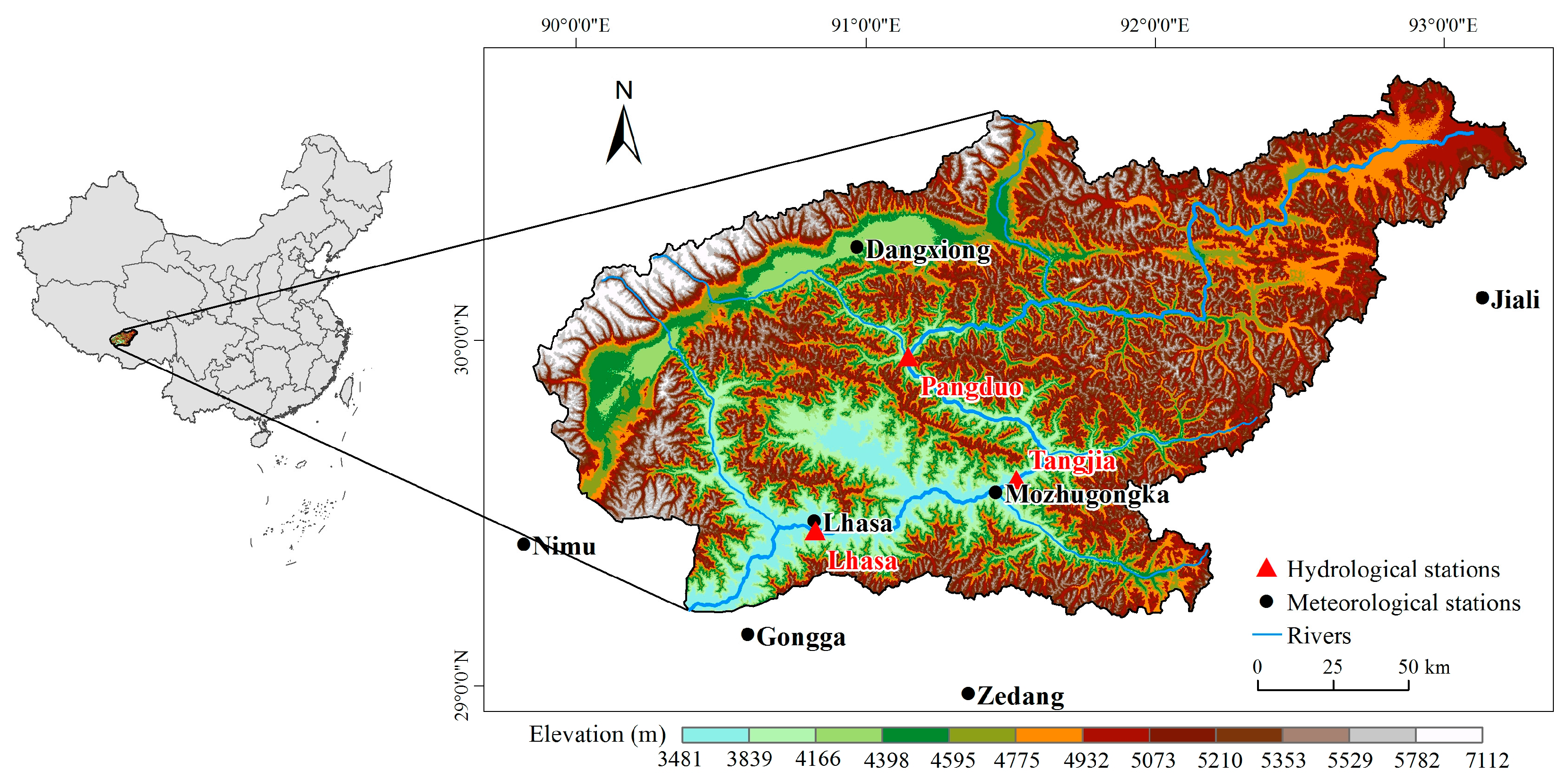
2.1. Study Area

The Lhasa River Basin (29°20′ N–31°15′ N, 90°05′ E–93°20′ E) lies at the south-eastern part of the Tibetan Plateau (Figure 1), which is one of the most sensitive areas to global climate change [20,21]. The total area of the Lhasa River Basin is approximately 32,600 km², and its altitude ranges from 3481 to 7112 m above sea level. Alpine meadow, alpine steppe, sparse grassland, and shrub are the main vegetation types. The mean annual temperature ranges from −1.5 °C to 7.8 °C and annual precipitation ranges from 340 to 700 mm. However, the distribution of precipitation is extremely temporally uneven, as about 90% of it occurs during June to September.

The Lhasa River Basin is the economic, agricultural, and demographic center of the Tibet Autonomous Region. Meeting domestic and agricultural water demand relies almost entirely on the water yield from the basin through surface and groundwater systems. According to the Integrated Planning for the Lhasa River Basin 2000–2020 [27], although the Basin’s water resources are quite abundant with an average annual runoff of the Lhasa River of about 1.04 × 10¹⁰ m³, water shortages still exist due to unevenly distributed precipitation and lack of sufficient water conservation facilities. With Lhasa city being the provincial capital of the Tibet Autonomous Region located downstream, the Lhasa River Basin is facing increasing pressures from human activities including urbanization, overgrazing, and tourism.

2.2. Seasonal Water Yield Model

This model is a spatially-explicit model working at the spatial resolution of the input DEM (Digital Elevation Model) raster. Thus, all the spatial results generated in this study are at the resolution of 30 m. The key model functions extracted from the model handbook [6] are as follows.

2.2.1. Quick Flow

Quick flow refers to the rainfall that leaves land surface quickly, versus infiltrating into the soil to produce local recharge. It is calculated using a CN-based approach, and an exponential distribution of the daily precipitation depths on days with rain is assumed:

$$Q{F}_{i,m}=R{E}_{i,m}\times \left(\left(a_{i,m}-S_i\right)exp\left(-\frac{0.2S_i}{a_{i,m}}\right)+\frac{S_i^2}{a_{i,m}}exp\left(\frac{0.8S_i}{a_{i,m}}\right)E_1\left(\frac{S_i}{a_{i,m}}\right)\right)\times \left(25.4\left[\frac{mm}{in}\right]\right)$$

(1)

where $R{E}_{i,m}$ is the number of rain events at pixel i in month m; $a_{i,m}$ is the mean rain depth on a rainy day at pixel i on month m; $S_i=\frac{1000}{C{N}_i}-10$; $C{N}_i$ is the curve number for pixel i; and $E_1$ is the exponential integral function. Furthermore, in the boundary case, a stream cell’s quick flow is set to the precipitation at that cell. The annual quick flow $Q{F}_i$ is then calculated from the sum of monthly values $Q{F}_{i,m}$.

2.2.2. Local Recharge

The local recharge, or potential contribution to baseflow, is computed from the local water balance. Local recharge can be negative if a pixel uses up gradient subsidies to satisfy its water demand. The local recharge index is computed on an annual time scale, but uses values derived from monthly water budgets. For a pixel i, the local recharge derived from the annual water budget is:

$$L_i=P_i-Q{F}_i-AE{T}_i$$

(2)

where$L_i$ is the local recharge derived from the annual water budget for pixel i;$P_i$ is the annual precipitation for pixel i; and $AE{T}_i$ is the annual actual evapotranspiration for pixel i, and is the sum of monthly evapotranspiration. For each month,$AE{T}_{i,m}$ is either limited by the demand or by the available water:

$$AE{T}_{i,m}=min\left(PE{T}_{i,m};P_{i,m}-Q{F}_{i,m}+{\alpha }_m{\beta }_i{L}_{sum.avail,i}\right)$$

(3)

where${\alpha }_m$ is the fraction of upslope annual available recharge that is available in month m (default is 1/12);${\beta }_i$ is the fraction of the upgradient subsidy that is available for down gradient evapotranspiration (default is 1);$L_{sum.avail,i}$ is the upslope annual available recharge for pixel i, and it is recursively computed according to the relationship of pixel i and its surrounding cells; and$PE{T}_{i,m}$ is the monthly potential evapotranspiration:

$$PE{T}_{i,m}=K_{c,i,m}\times E{T}_{0,i,m}$$

(4)

where$E{T}_{0,i,m}$ is the reference evapotranspiration for month m; and$K_{c,i,m}$ is the monthly crop factor for the pixel’s land cover type.

2.2.3. Baseflow

The baseflow calculated by this model represents the actual contribution of a pixel to baseflow (i.e., water that reaches the stream). If the local recharge is negative, then the pixel does not contribute to the baseflow and thus its baseflow is set to zero. If the pixel contributes to groundwater recharge, then its baseflow is a function of the amount of flow leaving the pixel and of the relative contribution to recharge of this pixel.

For a parcel that is not adjacent to the stream channel, the cumulative baseflow, $B_{sum,i}$, is proportional to the cumulative baseflow leaving the adjacent down gradient parcels minus the cumulative baseflow that is generated on that same down gradient parcel:

$$B_{sum,i}=L_{sum,i},\mathrm{if}j\mathrm{is}\mathrm{a}\mathrm{nonstream}\mathrm{pixel}$$

(5)

$$\mathrm{or}{B}_{sum,i}=L_{sum,i}{\sum }_{j\in \left\{cells to which cell i pours\right\}}{p}_{ij},\mathrm{if}j\mathrm{is}\mathrm{a}\mathrm{stream}\mathrm{pixel}$$

(6)

where$L_{sum,i}$ is the cumulative upstream recharge;$p_{ij}$ is the proportion of flow from cell i to j; and the baseflow$B_i$can be directly derived from the proportion of the cumulative baseflow leaving cell i, with respect to the available recharge to the upstream cumulative recharge:

$$B_i=\max \left(B_{sum,i}·\frac{L_i}{L_{sum,i}}, 0\right)$$

(7)

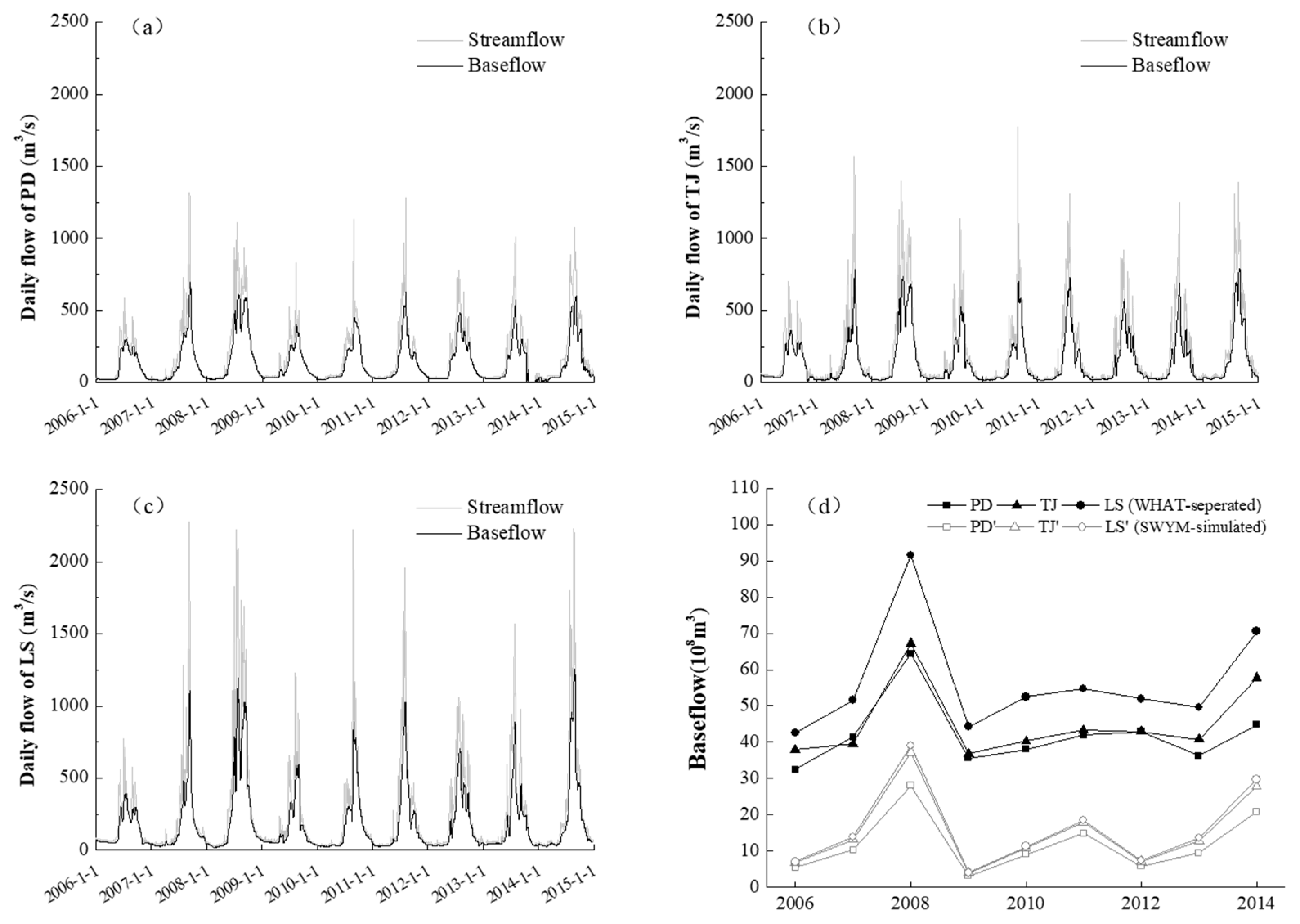
2.3. Baseflow Separation

The automated Web-Based Hydrograph Analysis Tool (WHAT) [28] was used to estimate the baseflow from the observed streamflow data. This tool includes three separation filters, and the Eckhardt Recursive Digital Filter method [29] was used on daily streamflow for baseflow separation in this study. This filter has been validated and widely used in similar analyses, and the algorithm has been shown to be robust for baseflow separation in various climatic and physiographic conditions [28,30,31,32]. Its mathematical expression is:

$$b_t=\frac{\left(1-BF{I}_{max}\right)\times \alpha +b_{t-1}+\left(1-\alpha \right)\times BF{I}_{max}\times Q_t}{1-\alpha \times BF{I}_{max}}$$

(8)

where$b_t$ is the filtered base flow at the t time step (m³/s); t is the time step number;$BF{I}_{max}$is the maximum baseflow index that can be modeled by the algorithm;$\alpha$is the filter parameter; and$Q_t$is the total streamflow at time step t (m³/s). Here, the suggested value of 0.98 for the filter parameter and 0.80 for$BF{I}_{max}$were selected according to the hydrogeological conditions of the study area and related research [28,30,31,32].

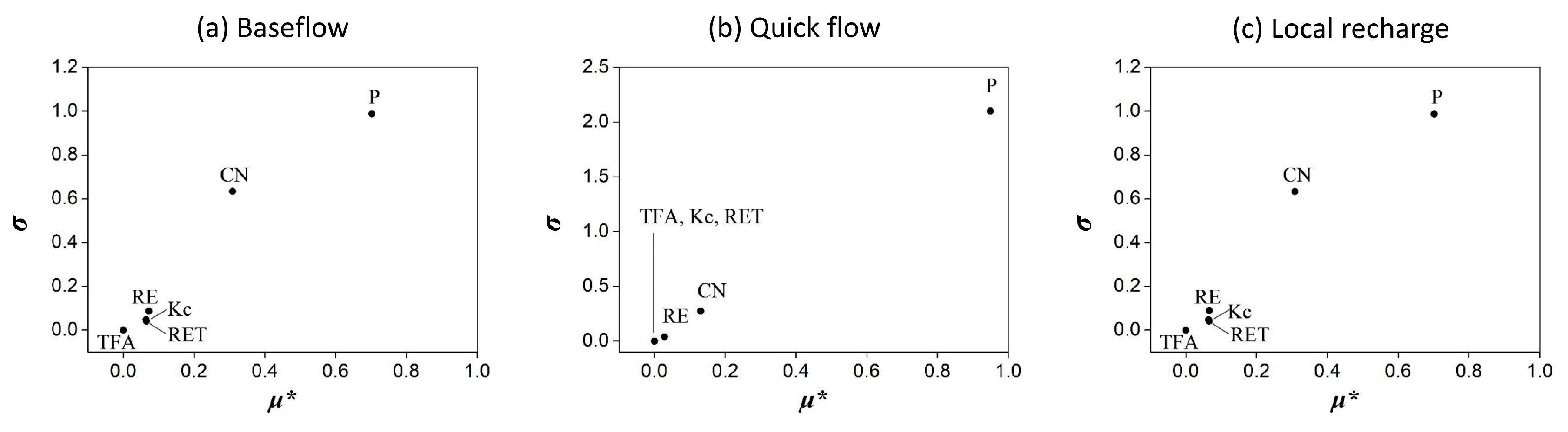
2.4. Sensitivity Analysis: Morris Screening Method

Sensitivity analysis is an essential and effective approach to examine the influence of model input changes on its output results. To date, many sensitivity analysis methods have been developed and improved including global sensitivity methods such as Sobol’s method [33,34] and Fourier Amplitude Sensitivity Testing (FAST) [35,36] as well as local sensitivity methods such as one-factor-at-a-time (OAT) [17,37]. In this study, the Morris screening method was applied, which is based on the replicated and randomized one-factor-at-a-time design [38]. Relying on a discrete partitioning of the factor space, this method has an improved economy of the computation by re-using some of the samples [39]. It computes the so-called elementary effects ($E{F}_i$) by taking the relative difference of the model output with and without a perturbation Δ of the ith factor:

$$E{F}_i=\frac{Y\left(x_1,x_2,\dots .,x_{i+\Delta },\dots ,x_k\right)-Y\left(x_1,x_2,\dots ,x_k\right)}{\Delta }$$

(9)

The calculation of $E{F}_i$ is replicated r times at randomly sampled points in the input space, leading to a distribution of $E{F}_i$ to infer a global sensitivity analysis. Then, the absolute means of distribution (${\mu }_i^{*}$) is calculated as a measure of importance and the standard deviation (${\sigma }_i$) as a measure of nonlinearity and/or interactions:

$${\mu }_i^{*}=\frac{1}{r}\sum \left|E{F}_i\right|$$

(10)

$${\sigma }_i=\sqrt{\frac{1}{r}\sum {\left(E{F}_i-{\mu }_i^{*}\right)}^2}$$

(11)

To compare the elementary effects taking into account the original scale of variation for each parameter, it is advised to scale the elementary effects with the standard deviation of the input ${\sigma }_{x_i}$ and of the output ${\sigma }_y$ [40]:

$$SE{F}_i=\frac{{\sigma }_{x_i}}{{\sigma }_y}\frac{{\Delta }_y}{{\Delta }_{x_i}}$$

(12)

In this study, we divided each parameter space into 10 levels, and replicated each elementary effect calculation 10 times (r = 10). The variation range of the six model inputs are listed in

Table 1. Variation range of model inputs in the sensitivity analysis.

No.	Parameters	Definition	Range	Unit
1	Precipitation (P)	Average annual precipitation	(50, 500)	mm
2	Reference evapotranspiration (RET)	Potential evaporation of a hypothetical vegetation with an abundant water supply	(50, 500)	mm
3	Curve number (CN)	An empirical parameter used in hydrology for predicting direct runoff or infiltration from rainfall excess	(10, 100)	-
4	Crop/vegetation coefficient (Kc)	Properties of plants used in predicting evapotranspiration	(0.1, 1)	-
5	Threshold flow accumulation (TFA)	The number of upstream cells that must flow into a cell before it is considered part of a stream	(1000, 10000)	-
6	Rain events (RE)	Average number of monthly rain events	(2, 20]	-

, referring to previous sensitivity analysis studies on the InVEST annual water yield model [17,18,19]. To simplify the sensitivity analysis process, all monthly inputs including P, RET, CN, Kc, and RE were set to have the same value for each month.

2.5. Quantifying Relative Contributions of Influencing Factors

To understand the relative influence of each factor on water yield changes, three scenarios were simulated during each time period in which each time only one factor was changed: (1) only precipitation changed; (2) only land cover changed; and (3) only NDVI changed. The change of water yield (including baseflow, local recharge, and quick flow) resulted from the changing factor, then equaled the difference of simulated water yield and the actual water yield in that period.

2.6. Data Sources

Precipitation data from 1955 to 2015 was used for analyzing the historical climate change trend, and among which the data from 1990 to 2015 was used for water yield modeling (spatially interpolated from site observation data to 30 m resolution raster data through the Kriging method). Land cover was categorized into ten types based on the revised classification system of the China Cover dataset [41] to better reflect local vegetation cover characteristics: forest, shrub, alpine meadow, alpine steppe, sparse grassland, farmland, barren land, artificial surface, water, and snow/glacier. Average annual growing season NDVI (from June to October) of each vegetation cover type was calculated to analyze the ecosystem quality change. The daily stream flow data of three hydrologic stations were used to verify the reliability of the SWYM.

Additional data used in the SWYM included: (1) DEM (Digital Elevation Model); (2) soil texture data, which were used to classify the SCS (Soil Conservation Service) soil hydrologic groups [42]; (3) CN (curve number) value for each land cover type, referenced from the USDA (United States Department of Agriculture) handbook [42] and adjusted by relevant studies in China [43,44]; (4) monthly Kc (crop/vegetation coefficient) values. For non-vegetated land cover types, the Kc values were obtained from the FAO (Food and Agriculture Organization Food and Agriculture Organization of the United Nations) guidelines [45] and the InVEST handbook [6], for vegetated land cover types, the Kc values were estimated using leaf area index (LAI) relationships [45] and the monthly LAI for each vegetated land cover type was calculated using NDVI data [46]; and (5) monthly reference evapotranspiration data. Detailed data information and sources are listed in

Table 2. Data information and sources.

Name	Data Type	Resolution	Time Availability	Source
Precipitation	Excel	-	1955–2015, monthly	China Meteorological Data Service Center
Land cover	Raster	30 m	1990, 2000, 2010, 2015	Institute of Remote Sensing and Digital Earth, Chinese Academy of Sciences
NDVI	Raster	250 m	1990, 2000, 2010, 2015	Institute of Remote Sensing and Digital Earth, Chinese Academy of Sciences
Stream flow	Excel	-	2006–2014, daily	China Institute of Water Resources and Hydropower Research
DEM	Raster	30 m	2015	Geospatial Data Cloud (http://www.gscloud.cn/)
Soil texture	Raster	1 km	-	Harmonized World Soil Database (http://www.fao.org/soils-portal/soil-survey/soil-maps-and-databases/harmonized-world-soil-database-v12/zh/)
CN	Excel	-	-	USDA (United States Department of Agriculture) handbook [42]
Kc	Excel	-	-	FAO (Food and Agriculture Organization of the United Nations) guidelines [45]
Reference evapotranspiration	Raster	1 km	Monthly	CGIAR CSI dataset (https://cgiarcsi.community/)

.

3. Results

3.1. Sensitivity Analysis and Model Validation

The absolute means (μ^*) and standard deviations (σ) of the elementary effect distribution are plotted in Figure 2 for the three model outputs: baseflow, quick flow, and local recharge. For baseflow and local recharge, their sensitivity factors were nearly the same: P and CN were the two most important factors, also with high σ values indicating the presence of non-linearity and/or interactions with other factors; RE, Kc, and RET were less important factors and also have less non-linearity and/or fewer interactions; TFA was identified as being non-influential with almost zero importance. For quick flow, P was the most important factor with the highest non-linearity and/or number of interactions, followed by CN and RE; TFA, Kc, and RET all had little influence on the quick flow output.

The baseflow of three hydrological stations was separated from the observed daily stream flow data to validate the model (Figure 3a–c). However, since the baseflow calculated by the SWYM only represents the contribution of a pixel to the baseflow, rather than the actual amount of baseflow, and our aim was to study the changing trend of water yield rather than its exact amount, the model was not calibrated by the observed data. Instead, the Pearson correlation analysis was used to compare the annual changing trend of the model simulated baseflow with the separated baseflow from the observed data. Results showed that the annual changing trend of the simulated baseflow was consistent with the separated baseflow (Figure 3d), and the separated and simulated baseflow values of the three sub watersheds were all significantly correlated (r_LS² = 0.960, r_TJ² = 0.956, r_PD² = 0.874; p < 0.01). These findings indicated that the simulated baseflow calculated by the SWYM can represent the annual variation characteristics of the actual baseflow.

3.2. Changing Trends of Influencing Factors

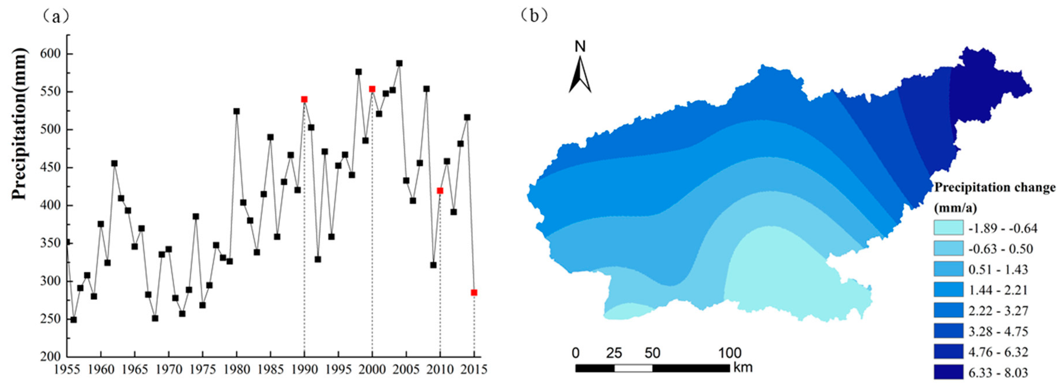
3.2.1. Precipitation

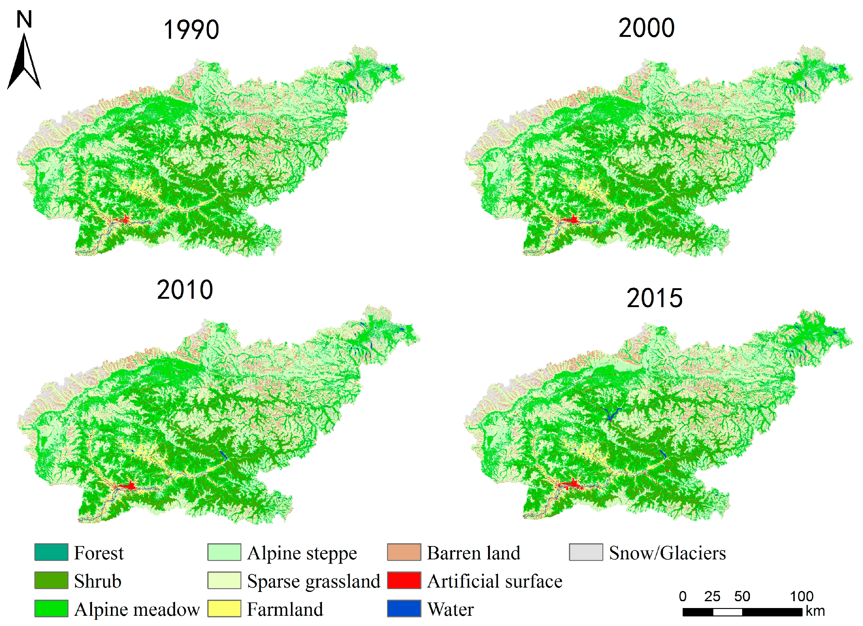
The precipitation records from the seven meteorological stations (locations shown in Figure 1) within and near the Lhasa River Basin were used to calculate the average annual precipitation (Figure 4a). There was an obvious increasing trend of precipitation from 1955 to 2004, although there were some large variations in the most recent 10 years, with extremely dry years such as 2009 and 2015 with precipitation <350 mm. Specifically, looking at the four years in which the water yield was assessed, there was a significant decrease in precipitation after 2000. In terms of spatial variation, the precipitation changing trend was inconsistent in the study area (Figure 4b). From north–east to south–west, the increasing trend became less substantial and the south-eastern area even showed a slight decreasing trend. Overall, the south-eastern area had become drier, and the north-eastern part had become wetter during the whole time period.

3.2.2. Land Cover

The main land cover types of the Lhasa River Basin are alpine meadow, alpine steppe, and sparse grassland, and more than 70% of the study area consisted of these (Figure 5,

Table 3. Area of different land cover types and changing rate in the Lhasa River Basin from 1990 to 2015 (Unit: km²).

Land Cover Type	1990	2000	2010	2015*	Area Change in Land Cover between 1990 and 20151	Proportion Change in Land Cover between 1990 and 2015
Forest	80.01	80.21	80.73	80.75	0.74	0.92%
Shrub	5077.63	5077.64	5077.72	5065.31	−12.33	−0.24%
Alpine meadow	8561.66	8562.13	8561.94	8682.04	120.38	1.41%
Alpine steppe	7629.94	7631.09	7613.59	7702.02	72.09	0.94%
Sparse grassland	7388.28	7400.13	7401.72	7152.10	−236.19	−3.20%
Farmland	613.00	598.68	584.79	583.83	−29.17	−4.76%
Barren land	2098.49	2104.65	2105.12	2108.88	10.39	0.50%
Artificial surface	90.29	102.97	117.59	164.87	74.57	82.59%
Water	174.65	174.42	188.70	231.07	56.42	32.30%
Snow/Glaciers	964.57	946.62	946.62	860.31	−104.26	−10.81%

Since the boundary of the original land cover data of 2015 was slightly different than in previous years, there is a missing area of 47.34 km² in the total area in 2015.

). From 1990 to 2015, the most substantial change was the rapid expansion of artificial surface and water area, which increased by 82.65% and 32.40% respectively, although their area was very small, together only accounting for 1.22% of the whole basin area in 2015. The area of alpine meadow and alpine steppe increased by 120.09 km² and 88.43 km², respectively, accounting for 0.36% and 0.27% of the whole basin. The area of sparse grassland and snow/glaciers decreased by 249.63 km² and 86.31 km², respectively, accounting for 0.75% and 0.26% of the whole basin. The other land cover types remained largely unchanged. Overall, the first twenty years from 1990 to 2010 saw few changes and the major land cover changes happened predominantly from 2010 to 2015.

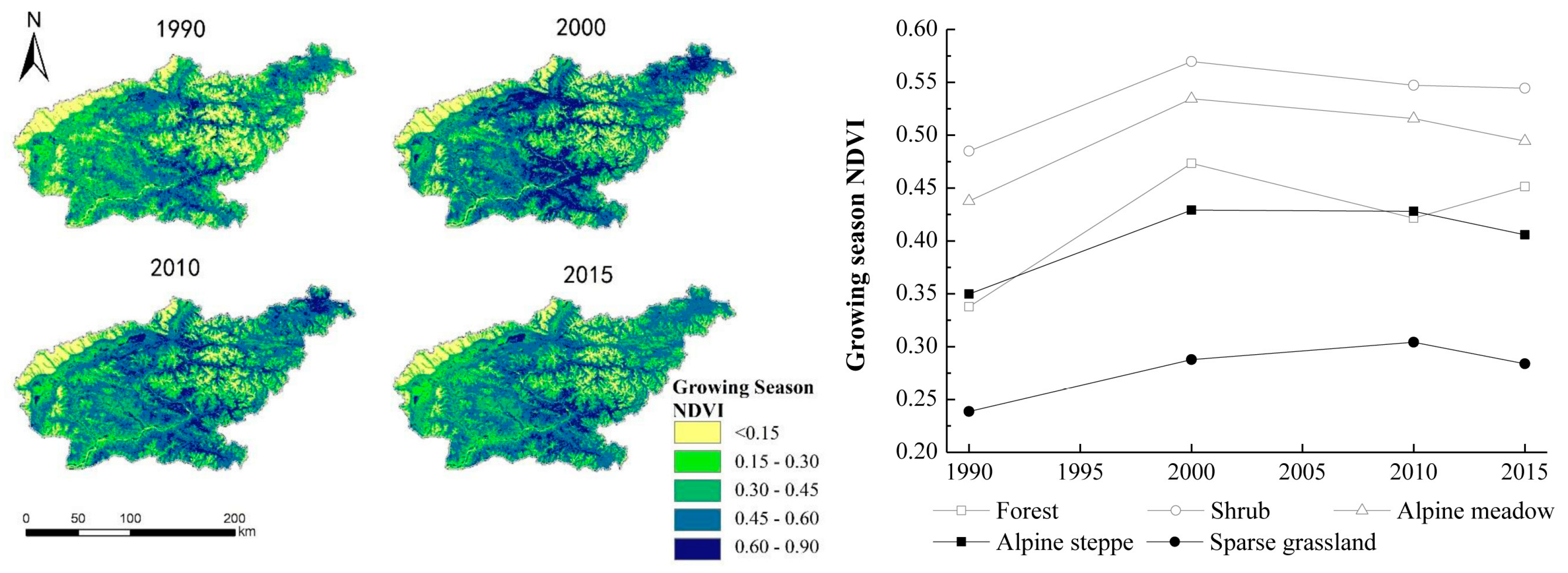
3.2.3. Normalized Difference Vegetation Index (NDVI)

From 1990 to 2000, the growing season NDVI of all vegetation types experienced sizeable increases, averagely increasing by 24.69%; from 2000 to 2010, the NDVI of forest, shrub, and alpine meadow decreased by 10.97%, 3.92%, and 3.52%, respectively, while the sparse grassland’s NDVI increased by 5.67%; from 2010 to 2015, the NDVI of forest increased by 7.10%, while the NDVI of sparse grassland, alpine steppe, and alpine meadow decreased by 6.66%, 5.16%, and 4.11% (Figure 6) respectively. Overall, from 1990 to 2000 all vegetation NDVI increased significantly, and the alpine meadow and alpine steppe have shown consistent decreasing trends since 2000.

3.3. Water Yield Change

The spatial distribution and statistical results of baseflow, local recharge, and quick flow from 1990 to 2015 are shown in Figure 7a–c, respectively. Through the whole period, the spatial pattern of water yield remained mostly unchanged. The north-eastern part of the basin, or the upstream area, had relatively high baseflow and local recharge values, and was also the main contributor to quick flow. The south-western part of the basin, or the downstream area, had relatively low or even zero baseflow, and most of its local recharge was negative due to high evapotranspiration. In terms of total water yield (Figure 7d), from 1990 to 2015, the baseflow, local recharge, and quick flow decreased by 67.03%, 80.21%, and 37.03%, respectively. The main change in the baseflow and local recharge occurred during 2000–2010, when they decreased by 67.43% and 83.35%, respectively; the annual variation of quick flow was relatively small.

3.4. Relative Contributions of Influencing Factors

Results showed that baseflow and local recharge were mainly affected by both precipitation and NDVI change, while the quick flow was mainly affected by precipitation (

Table 4. The individual contributions of precipitation, land cover, and NDVI change on water yield changes. ΔP is the contribution of precipitation change on water yield; ΔL is the contribution of land cover change; ΔN is the contribution of NDVI change (Unit: mm).

Time Period	1990–2000			2000–2010			2010–2015
Influencing Factor	ΔP	ΔL	ΔN	ΔP	ΔL	ΔN	ΔP	ΔL	ΔN
Δ Baseflow	22.80	−0.09 1	−25.78	−76.68	0.06	−3.46	1.77	−0.88	1.97
Δ Local Recharge	22.81	−0.09	−28.91	−90.74	0.08	−3.96	4.21	2.71	−0.67
Δ Quick flow	1.58	0.03	0.00	−8.93	0.01	0.00	−0.61	−0.03	0.00

¹ The negative sign (−) is used to represent a negative effect (i.e., a change resulting in a decrease in water yield).

). For baseflow, the influence of precipitation change was, on average, 7.98 times as big as the NDVI change during the three time periods, and the influence of NDVI change was, on average, 115.45 times as big as land cover change. For local recharge, the influence of precipitation change was on average, 9.99 times as big as NDVI change during the three time periods, and the influence of NDVI change was on average, 123.66 times as big as land cover change. It can be seen that precipitation is the main influencing factor that resulted in water yield change, while NDVI also played an important role and land cover change had little influence in the study area.

Through time, the main change of baseflow, local recharge, and quick flow happened during 2000–2010 due to the huge decrease of precipitation. During 1990–2000 and 2010–2015, precipitation change and NDVI change had nearly equivalent influences on baseflow. Land cover change began to exert a greater influence on local recharge and baseflow after 2010. For example, the influence of land cover change on local recharge was 0.64 times as big as precipitation cover change during 2010–2015.

4. Discussion

4.1. Model Performance and Uncertainties

The SWYM has been proven to be able to generate spatially explicit and reliable results of baseflow, local recharge, and quick flow, which can depict the seasonal flow characteristics. This represents an advance on the previous annual water yield model, which can only depict the total water yield. In terms of model sensitivity, although the theory behind the two models is different, there are some similarities. Precipitation is the most sensitive factor to both seasonal and annual water yield models [17]. The CN value is the second most sensitive input in SWYM, where Z is another very important input in the annual water yield model. The sensitivity analysis results also correspond with the water yield results and relative contribution analysis, where precipitation change contributed most to the water yield change during the whole study period, especially between 2000 and 2010. Although this model was not calibrated in this study because it was developed to only quantify the relative contribution of different land covers, the correlation analysis with the observed data showed that the model results could represent the annual variation characteristics of the actual water yield.

Compared with other hydrological models such as SWAT, SWYM is relatively simple and easy to use with reduced data requirements. It can also be easily used to explore different scenarios such as climate and/or land use change. However, due to the simplified hydrological process in this model, the results could be unrealistic in certain cases [15]. Different data sources and resolutions as well as different spatial scales (national, provincial, or sub-watershed scales) may also strongly influence study findings [47]. Therefore, model calibration and validation with observed flow data should be carried out before assessment. Until now, this model has only been used in a few locations including East Africa, USA, Rwanda, and China [16,47,48,49], because it was only released in 2016 and its data requirement is a little higher than the InVEST annual water yield model. Monthly data of precipitation, reference evapotranspiration, Kc, and CN values are all required in SWYM. Nevertheless, it still has huge potential to be widely used in the future.

Inevitably, there are some uncertainties in the assessment in this study. First, the process of groundwater recharge and melting of ice and snow were neglected in the model, which is one possible reason for the discrepancy between the predicted baseflow and observed data in Figure 3d. Second, due to the lack of experimental studies on the relationship between CN values and vegetation indexes, the CN values for each vegetated land cover type were set as unchanged among different years. Water abstractions in the study area were also not considered due to a lack of data availability. Notwithstanding this recognition, the model was only used to assess the water yield variation and the relative contribution of precipitation, land cover, and NDVI changes, rather than to calculate the exact baseflow or quick flow, thus these limitations were considered acceptable in this study.

4.2. Driving Force Analysis: Climate Change and Human Activities in Combination

In this study, we analyzed the influence of three factors, namely precipitation change, land cover change, and NDVI change on water yield. Although these three factors are interconnected and their changes could be coincided, it is hard to disentangle their influence on each other. Therefore, in this study, it was assumed that these three changing factors are independent. However, they are all under the same driving forces: climate change and human activities. Understanding the mechanism of the underlying driving forces is crucial for making management-level strategies.

The results showed that precipitation was the main factor influencing the water yield, followed by NDVI, while land cover change began to exert greater influence after 2010. Since precipitation change is one of the main characteristics of climate change, this result confirmed that climate change and land cover change are the main driving forces of ecosystem services, as indicated in many previous studies [3,9,50,51]. It is widely suggested that land cover/use change is strongly dominated by human activities such as urbanization and agricultural expansion [52,53,54,55,56]. NDVI change, which is the index of vegetation variation, however, is affected by both climate change and human activities, and their influences are usually combined and interact. Climate change can lead to the loss or increase in growth, biomass, or diversity at the level of species populations, interspecific relationships, landscapes, or entire biomes [57]; while human activities such as overgrazing and species invasion can also directly change the vegetation status.

Many studies have revealed the relative contribution of climate change and human activities to vegetation variation in the Tibetan Plateau. Pan et al. [25] indicated that in the Tibetan Plateau, the impacts of non-climatic drivers on grassland variations were approximately twice as intense as that of the climatic drivers in the past three decades. Xu et al. [58] demonstrated that the percentage area of NPP change of alpine grassland in the Tibetan Plateau induced by climatic factors increased from 41.55% to 83.75%, but that the percentage change caused by human activities decreased from 58.45% to 16.25% in the two periods of 2000–2004 and 2004–2012. Chen et al. [59] indicated that the percentage area of actual grassland NPP change caused by climate change declined from 79.62% to 56.59% in the two periods of 1982–2001 and 2001–2011, respectively; but that the percentage change resulting from human activities doubled from 20.16% to 42.98% in the same periods over the Qinghai-Tibet Plateau. Although the results of these studies differed from each other due to the use of different data sources and model parameters, and the mechanisms of how climate change and human activities jointly affect the ecosystem remain unclear [60], it is evident from our findings and the literature that both climate change and human activities play important roles in shaping grassland variations in the Tibetan Plateau. This suggests that where such changes are undesirable, policies and other interventions would need to target both climate change and human aspects in order to address the changes.

Climate change in the Lhasa River Basin, as focused on through changing precipitation, was substantial compared to the average global and Tibetan Plateau trends. Additionally, the intensity of human activities in the Lhasa River Basin has also increased over the past three decades, despite the local government having already developed and enacted various environmental protection practices such as the Grassland Subsidy Policy for grassland restoration. The speed of urbanization in the downstream area has been increasing rapidly, as have the activities of the tourism sector. Based on the statistics from the Tibet Statistical Yearbook [61], from 1990 to 2014, the GDP of the Lhasa River Basin increased from 0.75 billion Yuan to 34.74 billion Yuan, while the total population increased from 0.76 million to 1.09 million. The increasing GDP and population means a greater water demand in domestic and agricultural use in the future as well as more demand for hydropower, the major source of electricity in the basin. All these demands rely on the water yield ecosystem service. The Lhasa River Basin is also very rich in mineral resources. Some of the mineral processing plants are located close to the sensitive ecosystems in the upper reaches of the river basin, which is the main contributor of water yield, especially for baseflow (Figure 7a), and mining activities might therefore have a long-term impact on the ecosystem unless they are more closely investigated and managed. Furthermore, exploitive overstocking of livestock is still widespread across the Tibetan Plateau [62,63]. The vegetation losses resulting from overgrazing will lead to enhanced soil erosion and sedimentation. Sustainable grazing management taking into account the impacts on vegetation and changing climatic conditions should be promoted to livestock keepers.

5. Conclusions

The SWYM has been proven to be an efficient tool for revealing the effects of climate, land cover, and NDVI change on water yield by delivering the spatial results of baseflow, local recharge, and quick flow, which together depicts the seasonal flow characteristics. According to relative contribution analysis, baseflow and local recharge were mainly affected by precipitation and NDVI change in the Lhasa River Basin over the study period, while the quick flow was mainly affected by precipitation. Additionally, land cover change began to exert greater influence after 2010. While climate change and land cover change are widely studied and recognized as two of the main driving forces on ecosystem services, this study showed that the vegetation change, which is usually driven by both climate change and human activities, is also important in terms of water yield. For the Lhasa River Basin, the monitoring and management of hydrological processes should be strengthened, and management strategies that explicitly take into account rapidly changing climate and human activities should be developed.

References

1. Fan, M.; Shibata, H. Spatial and temporal analysis of hydrological provision ecosystem services for watershed conservation planning of water resources. Water Resour. Manag. 2014, 28, 3619–3636. [Google Scholar] [CrossRef]
2. Muthuwatta, L.; Amarasinghe, U.A.; Sood, A.; Lagudu, S. Reviving the “Ganges Water Machine”: Where and how much? Hydrol. Earth Syst. Sci. 2017, 12, 9741–9763. [Google Scholar] [CrossRef]
3. Qin, J.; Ding, Y.J.; Han, T.D.; Liu, Y.X. Identification of the factors influencing the baseflow in the permafrost region of the Northeastern Qinghai-Tibet Plateau. Water 2017, 9, 666. [Google Scholar] [CrossRef]
4. Maliehe, M.; Mulungu, D.M.M. Assessment of water availability for competing uses using SWAT and WEAP in South Phuthiatsana catchment, Lesotho. Phys. Chem. Earth 2017, 100, 305–316. [Google Scholar] [CrossRef]
5. Yao, Y.; Zheng, C.; Andrews, C.; Zheng, Y.; Zhang, A.; Liu, J. What controls the partitioning between baseflow and mountain block recharge in the Qinghai-Tibet Plateau? Geophys. Res. Lett. 2017, 44, 8352–8358. [Google Scholar] [CrossRef]
6. Sharp, R.; Tallis, H.T.; Ricketts, T.; Guerry, A.D.; Wood, S.A.; Chaplin-Kramer, R.; Nelson, E.; Ennaanay, D.; Wolny, S.; Olwero, N.; et al. VEST 3.3.3. User’s Guide. 2016. Available online: http://data.naturalcapitalproject.org/nightly-build/invest-users-guide/html/ (accessed on 21 May 2020).
7. Mandle, L.; Wolny, S.; Hamel, P.; Project, N.C.; Helsingen, H.; WWF-Myanmar; Bhagabati, N.; Dixon, A.; WWF-US. Natural Connections: How Natural Capital Supports Myanmar’s People and Economy. 2016. Available online: https://www.worldwildlife.org/publications/natural-connections-how-natural-capital-supports-myanmar-s-people-and-economy (accessed on 21 May 2020).
8. Santhi, C.; Allen, P.M.; Muttiah, R.S.; Arnold, J.G.; Tuppad, P. Regional estimation of base flow for the conterminous United States by hydrologic landscape regions. J. Hydrol. 2008, 351, 139–153. [Google Scholar] [CrossRef]
9. Ahiablame, L.; Sheshukov, A.Y.; Rahmani, V.; Moriasi, D. Annual baseflow variations as influenced by climate variability and agricultural land use change in the Missouri River Basin. J. Hydrol. 2017, 551, 188–202. [Google Scholar] [CrossRef] [Green Version]
10. Zomlot, Z.; Verbeiren, B.; Huysmans, M.; Batelaan, O. Spatial distribution of groundwater recharge and base flow: Assessment of controlling factors. J. Hydrol. Reg. Stud. 2015, 4, 349–368. [Google Scholar] [CrossRef] [Green Version]
11. Jiang, C.; Li, D.Q.; Wang, D.W.; Zhang, L.B. Quantification and assessment of changes in ecosystem service in the Three-River Headwaters Region, China as a result of climate variability and land cover change. Ecol. Indic. 2016, 66, 199–211. [Google Scholar] [CrossRef]
12. Wang, H.; Sun, F.; Xia, J.; Liu, W. Impact of LUCC on streamflow based on the SWAT model over the Wei River basin on the Loess Plateau in China. Hydrol. Earth Syst. Sci. 2017, 21, 1–30. [Google Scholar] [CrossRef] [Green Version]
13. Gao, H.; Tang, Q.; Shi, X.; Zhu, C.; Bohn, T.; Su, F.; Pan, M.; Sheffield, J.; Lettenmaier, D.; Wood, E. Water Budget Record from Variable Infiltration Capacity (VIC) Model. In Algorithm Theoretical Basis Document for Terrestrial Water Cycle Data Records. 2010. Available online: http://hydrology.princeton.edu/~mpan/academics/uploads/content/articles/Water_Cycle_MEaSUREs_ATBD_Combined_v1.0.pdf (accessed on 21 May 2020).
14. Sun, F.; Mejia, A.; Che, Y. Disentangling the Contributions of Climate and Basin Characteristics to Water Yield across Spatial and Temporal Scales in the Yangtze River Basin: A Combined Hydrological Model and Boosted Regression Approach. Water Resour. Manag. 2019, 33, 3449–3468. [Google Scholar] [CrossRef]
15. Scordo, F.; Lavender, T.; Seitz, C.; Perillo, V.; Rusak, J.; Piccolo, M.; Perillo, G. Modeling water yield: Assessing the role of site and region-specific attributes in determining model performance of the InVEST Seasonal Water Yield Model. Water 2018, 10, 1496. [Google Scholar] [CrossRef] [Green Version]
16. Yang, S.Q.; Zhao, W.W.; Liu, Y.X.; Wang, S.; Wang, J.; Zhai, R.J. Influence of land use change on the ecosystem service trade-offs in the ecological restoration area: Dynamics and scenarios in the Yanhe watershed, China. Sci. Total Environ. 2018, 644, 556–566. [Google Scholar] [CrossRef]
17. Redhead, J.W.; Stratford, C.; Sharps, K.; Jones, L.; Ziv, G.; Clarke, D.; Oliver, T.H.; Bullock, J.M. Empirical validation of the InVEST water yield ecosystem service model at a national scale. Sci. Total Environ. 2016, 569, 1418–1426. [Google Scholar] [CrossRef] [Green Version]
18. Sánchez-Canales, M.; López Benito, A.; Passuello, A.; Terrado, M.; Ziv, G.; Acuña, V.; Schuhmacher, M.; Elorza, F.J. Sensitivity analysis of ecosystem service valuation in a Mediterranean watershed. Sci. Total Environ. 2012, 440, 140–153. [Google Scholar] [CrossRef]
19. Hamel, P.; Guswa, A.J. Uncertainty analysis of a spatially explicit annual water-balance model: Case study of the Cape Fear basin, North Carolina. Hydrol. Earth Syst. Sci. 2015, 19, 839–853. [Google Scholar] [CrossRef] [Green Version]
20. Pan, T.; Zou, X.T.; Liu, Y.J.; Wu, S.H.; He, G.M. Contributions of climatic and non-climatic drivers to grassland variations on the Tibetan Plateau. Ecol. Eng. 2017, 108, 307–317. [Google Scholar] [CrossRef]
21. Liu, X.D.; Chen, B.D. Climatic warming in the Tibetan plateau during recent decades. Int. J. Climatol. 2000, 20, 1729–1742. [Google Scholar] [CrossRef]
22. Yan, Y.; Zhang, Y.J.; Shan, P.; Zhao, C.L.; Wang, C.X.; Deng, H.B. Snow cover dynamics in and around the Shangri-La County, southeast margin of the Tibetan Plateau, 1974–2012: The influence of climate change and local tourism activities. Int. J. Sust. Dev. World 2015, 22, 156–164. [Google Scholar] [CrossRef] [Green Version]
23. Kang, S.C.; Xu, Y.W.; You, Q.L.; Flügel, W.A.; Pepin, N.; Yao, T.D. Review of climate and cryospheric change in the Tibetan Plateau. Environ. Res. Lett. 2010, 5, 015101. [Google Scholar] [CrossRef]
24. Xu, Z.X.; Gong, T.L.; Li, J.Y. Decadal trend of climate in the Tibetan Plateau—Regional temperature and precipitation. Hydrol. Process. 2008, 22, 3056–3065. [Google Scholar] [CrossRef]
25. Tao, J.; Zhang, Y.J.; Dong, J.W.; Fu, Y.; Zhu, J.T.; Zhang, G.L.; Jiang, Y.B.; Tian, L.; Zhang, X.Z.; Zhang, T. Elevation-dependent relationships between climate change and grassland vegetation variation across the Qinghai-Xizang Plateau. Int. J. Climatol. 2015, 35, 1638–1647. [Google Scholar] [CrossRef] [Green Version]
26. Wang, P.; Lassoie, J.P.; Morreale, S.J.; Dong, S.K. A critical review of socioeconomic and natural factors in ecological degradation on the Qinghai-Tibetan Plateau, China. Rangel. J. 2015, 37, 1–9. [Google Scholar] [CrossRef]
27. Tibet Autonomous Region Water Resources Planning Survey Design Institute. Integrated Planning for the Lhasa River Basin 2000–2020; Tibet Autonomous Region: Tibet, China, 2002. (In Chinese) [Google Scholar]
28. Lim, K.J.; Engel, B.A.; Tang, Z.X.; Choi, J.; Kim, K.S.; Muthukrishnan, S.; Tripathy, D. Automated Web Gis based hydrograph analysis tool, WHAT. J. Am. Water Resour. Assoc. 2005, 41, 1407–1416. [Google Scholar] [CrossRef]
29. Eckhardt, K. How to construct recursive digital filters for baseflow separation. Hydrol. Process. 2005, 19, 507–515. [Google Scholar] [CrossRef]
30. Ahiablame, L.; Chaubey, I.; Engel, B.; Cherkauer, K.; Merwade, V. Estimation of annual baseflow at ungauged sites in Indiana USA. J. Hydrol. 2013, 476, 13–27. [Google Scholar] [CrossRef]
31. Eckhardt, K. A comparison of baseflow indices, which were calculated with seven different baseflow separation methods. J. Hydrol. 2008, 352, 168–173. [Google Scholar] [CrossRef]
32. Combalicer, E.; Lee, S.; Ahn, S.; Kim, D.; Im, S. Comparing groundwater recharge and base flow in the Bukmoongol small-forested watershed, Korea. J. Earth Syst. Sci. 2008, 117, 553–566. [Google Scholar] [CrossRef] [Green Version]
33. Sobol’, I.M. Sensitivity estimates for nonlinear mathematical models. Math. Model. Comput. Exp. 1993, 1, 407–417. [Google Scholar]
34. Zhang, C.; Chu, J.G.; Fu, G.T. Sobol’s sensitivity analysis for a distributed hydrological model of Yichun River Basin, China. J. Hydrol. 2013, 480, 58–68. [Google Scholar] [CrossRef] [Green Version]
35. McRae, G.J.; Tilden, J.W.; Seinfeld, J.H. Global sensitivity analysis—A computational implementation of the Fourier Amplitude Sensitivity Test (FAST). Comput. Chem. Eng. 1982, 6, 15–25. [Google Scholar] [CrossRef] [Green Version]
36. Neumann, M.B. Comparison of sensitivity analysis methods for pollutant degradation modelling: A case study from drinking water treatment. Sci. Total Environ. 2012, 433, 530–537. [Google Scholar] [CrossRef] [PubMed]
37. Redhead, J.W.; May, L.; Oliver, T.H.; Hamel, P.; Sharp, R.; Bullock, J.M. National scale evaluation of the InVEST nutrient retention model in the United Kingdom. Sci. Total Environ. 2018, 610, 666–677. [Google Scholar] [CrossRef]
38. Morris, M.D. Factorial sampling plans for preliminary computational experiments. Technometrics 1991, 33, 161–174. [Google Scholar] [CrossRef]
39. Zhan, C.S.; Song, X.M.; Xia, J.; Tong, C. An efficient integrated approach for global sensitivity analysis of hydrological model parameters. Environ. Model. Softw. 2013, 41, 39–52. [Google Scholar] [CrossRef]
40. Sin, G.; Gernaey, K. Improving the Morris method for sensitivity analysis by scaling the elementary effects. In Proceedings of the 19th European Symposium on Computer Aided Process Engineering, Cracow, Poland, 14–17 June 2009. [Google Scholar]
41. Zhang, L.; Wu, B.F.; Li, X.S.; Xing, Q. Classification system of China land cover for carbon budget. Acta Ecol. Sin. 2014, 34, 7158–7166. (In Chinese) [Google Scholar]
42. United States Department of Agriculture (USDA). Chapter 7 Hydrologic Soil Groups, Part 630 Hydrology. In National Engineering Handbook; 2007. Available online: https://directives.sc.egov.usda.gov/OpenNonWebContent.aspx?content=22526.wba (accessed on 21 May 2020).
43. Guo, X.J.; Cui, P.; Zhuang, J.Q.; Liu, Y.H.; Zhang, J. SCS Model and Its application to rainfall-runoff in debris activity region—A case from Jiangjiagou watershed of Yunnan province. J. Soil Water Conserv. 2010, 30, 225–228. (In Chinese) [Google Scholar]
44. Zhou, C.N.; Ren, S.M.; Yan, M.J. Application of SCS model to simulate rainfall-runoff relationship in Wenyu river basin in Beijing. Trans. CSAE 2008, 24, 87–90. (In Chinese) [Google Scholar]
45. The Food and Agriculture Organization of the United Nations (FAO). Crop Evapotranspiration-Guidelines for Computing Crop Water Requirements-FAO Irrigation and Drainage Paper 56. 1998. Available online: http://www.fao.org/3/x0490e/x0490e00.htm (accessed on 21 May 2020).
46. Sun, P.S.; Liu, S.R.; Liu, J.T.; Liu, C.W.; Lin, Y.; Jiang, H. Derivation and validation of leaf area index maps using NDVI data of different resolution satellite imageries. Acta Ecol. Sin. 2006, 26, 3826–3834. [Google Scholar]
47. Bagstad, K.J.; Cohen, E.; Ancona, Z.H.; McNulty, S.G.; Sun, G. The sensitivity of ecosystem service models to choices of input data and spatial resolution. Appl. Geogr. 2018, 93, 25–36. [Google Scholar] [CrossRef]
48. Sahle, M.; Saito, O.; Fürst, C.; Yeshitela, K. Quantifying and mapping of water-related ecosystem services for enhancing the security of the food-water-energy nexus in tropical data–sparse catchment. Sci. Total Environ. 2019, 646, 573–586. [Google Scholar] [CrossRef]
49. Watson, K.B.; Galford, G.L.; Sonter, L.J.; Koh, I.; Ricketts, T.H. Effects of human demand on conservation planning for biodiversity and ecosystem services. Conserv. Biol. 2019, 33, 942–952. [Google Scholar] [CrossRef] [Green Version]
50. Pan, T.; Wu, S.H.; Liu, Y.J. Relative contributions of land use and climate change to water supply variations over Yellow River source area in Tibetan Plateau during the past three decades. PLoS ONE 2015, 10, e0123793. [Google Scholar] [CrossRef]
51. Su, C.H.; Fu, B.J. Evolution of ecosystem services in the Chinese Loess Plateau under climatic and land use changes. Glob. Planet. Chang. 2013, 101, 119–128. [Google Scholar] [CrossRef]
52. Falcucci, A.; Maiorano, L.; Boitani, L. Changes in land-use/land-cover patterns in Italy and their implications for biodiversity conservation. Landsc. Ecol. 2007, 22, 617–631. [Google Scholar] [CrossRef]
53. Nelson, E.; Sander, H.; Hawthorne, P.; Conte, M.; Ennaanay, D.; Wolny, S.; Manson, S.; Polasky, S. Projecting global land-use change and its effect on ecosystem service provision and biodiversity with simple models. PLoS ONE 2010, 5, e14327. [Google Scholar] [CrossRef] [Green Version]
54. Polasky, S.; Nelson, E.; Pennington, D.; Johnson, K.A. The impact of land-use change on ecosystem services, biodiversity and returns to landowners: A case study in the state of Minnesota. Environ. Resour. Econ. 2011, 48, 219–242. [Google Scholar] [CrossRef]
55. Intergovernmental Platform on Biodiversity and Ecosystem Services (IPBES). Summary for Policymakers of the Global Assessment Report on Biodiversity and Ecosystem Services of the Intergovernmental Science-Policy Platform on Biodiversity and Ecosystem Services. 2019. Available online: https://ipbes.net/global-assessment (accessed on 21 May 2020).
56. Intergovernmental Platform on Biodiversity and Ecosystem Services (IPBES). The IPBES Regional Assessment Report on Biodiversity and Ecosystem Services for Asia and the Pacifc. 2018. Available online: https://ipbes.net/assessment-reports/asia-pacific (accessed on 21 May 2020).
57. Intergovernmental Panel on Climate Change (IPCC). Chapter 1 Framing and Context. In Global Warming of 1.5°C; 2018; Available online: https://www.ipcc.ch/sr15/ (accessed on 21 May 2020).
58. Xu, H.J.; Wang, X.P.; Zhang, X.X. Alpine grasslands response to climatic factors and anthropogenic activities on the Tibetan Plateau from 2000 to 2012. Ecol. Eng. 2016, 92, 251–259. [Google Scholar] [CrossRef]
59. Chen, B.X.; Zhang, X.Z.; Tao, J.; Wu, J.S.; Wang, J.S.; Shi, P.L.; Zhang, Y.J.; Yu, C.Q. The impact of climate change and anthropogenic activities on alpine grassland over the Qinghai-Tibet Plateau. Agric. For. Meteorol. 2014, 189, 11–18. [Google Scholar] [CrossRef]
60. Reed, M.S.; Stringer, L.C. Land Degradation, Desertification, and Climate Change: Anticipating, Assessing, and Adapting to Future Change; Routledge: London, UK, 2016. [Google Scholar]
61. Tibet Autonomous Region Statistics Bureau. Tibet Statistical Yearbook; China Statistics Press: Beijing, China, 2015. [Google Scholar]
62. Dong, Q.M.; Zhao, X.Q.; Wu, G.L.; Chang, X.F. Optimization yak grazing stocking rate in an alpine grassland of Qinghai-Tibetan Plateau, China. Environ. Earth Sci. 2015, 73, 2497–2503. [Google Scholar] [CrossRef]
63. Harris, R.B. Rangeland degradation on the Qinghai-Tibetan plateau: A review of the evidence of its magnitude and causes. J. Arid Environ. 2010, 74, 1–12. [Google Scholar] [CrossRef]
Figure 1. The location of the Lhasa River Basin and the hydrological stations and meteorological stations in this area.
Water 12 01498 g001
Figure 2. Morris screening results: μ* indicates the importance and σ the degree of non-linearity or interaction caused by each factor for (a) baseflow, (b) quick flow and (c) local recharge: precipitation (P), curve number (CN), rain events (RE), crop/vegetation coefficient (Kc), reference evapotranspiration (RET), and threshold flow accumulation (TFA).
Water 12 01498 g002
Figure 3. (ac): The observed streamflow and WHAT (Web-Based Hydrograph Analysis Tool)-separated baseflow of the three hydrological stations from 2006–2014: Pangduo (PD), Tangjia (TJ), Lhasa (LS); (d) Comparison between the WHAT-separated and SWYM (Seasonal Water Yield Model)-simulated annual baseflow.
Water 12 01498 g003
Figure 4. (a) Annual mean precipitation (the red plots indicate the year 1990, 2000, 2010, and 2015) and (b) spatial precipitation changing trend in the Lhasa River Basin over the past six decades.
Water 12 01498 g004
Figure 5. Land cover change in the Lhasa River Basin from 1990 to 2015.
Water 12 01498 g005
Figure 6. Growing season normalized difference vegetation index (NDVI) distribution and changes of different vegetation types from 1990 to 2015.
Water 12 01498 g006
Figure 7. Spatial distribution of (a) baseflow, (b) local recharge, (c) quick flow, and (d) total amount.
Water 12 01498 g007aWater 12 01498 g007b