Automated Location Detection of Retention and Detention Basins for Water Management

Abstract

Retention and detention basins are engineering constructions with multiple objectives; e.g., flood protection and irrigation. Their performance is highly location-dependent, and thus, optimization strategies are needed. LOCASIN (Location detection of retention and detention basins) is an open-source MATLAB tool that enables automated and rapid detection, characterization and evaluation of basin locations. The site detection is based on a numerical raster analysis to determine the optimal dam axis orientation, the dam geometry and the basin area and volume. After selecting a reasonable basin combination, the results are summarized and visualized. LOCASIN represents a user-friendly and flexible tool for policy makers, engineers and scientists to determine dam and basin properties of optimized positions for planning and research purposes. It can be applied in an automated way to solve small and large scale engineering problems. The software is available on GitHub.

1. Introduction

Open source and user-friendly modeling and analysis tools play vital roles for engineers and decision-makers in water management [1,2]. In particular, the development of analysis tools for the management of floods and droughts is an important topic hydrologists are continuously dealing with [3,4]. Generally, one focus in flood management is the retention of water in a catchment for a defined period of time in order to reduce flood peaks and related hazards [5]. In contrast, the management of droughts requires having a source of stored water which can be used to meet the water demand in a region affected by a water shortage [6].

Despite having different main objectives, the management of floods and that of droughts have in common that the retention of water plays an important role. Depending on the size and specific characteristics of a catchment of interest, decision-makers may favor different sizes of detention basins, retention basins or reservoirs (from now on called basin). While large basins may be more appropriate as a flood protection measure for entire river catchments [7,8], small decentralized basins can play a supportive role in flood management for smaller subcatchments [9,10]. Similarly, those small basins or reservoirs have been shown to be effective in providing water for irrigation [11] or when being used for managed aquifer recharge [12]. Finding appropriate positions for all kinds of basins or reservoirs in a catchment independently from their respective size is an important task in water management for which specific and objective-oriented tools are needed. So far, different tools were proposed that were designed to find locations for flood detention basins [13,14,15,16,17,18], or for the optimization of irrigation reservoirs [19,20] or to select sites for managed aquifer recharge [21,22]. However, the level of detail of the results is often not appropriate for the evaluation of small basins, and the degree of automation could be improved in order to be applied for large-scale problems. Many studies analyze and evaluate spatial catchment characteristics such as land use, slope or geomorphology in order to determine suitable regions for the positioning of basins [13,14,15,18,21]. The local topography and the resulting dam or basin geometry are not covered in these analyses. Wimmer et al. [17] present a methodology for the automated determination of basin locations and characteristics based on an analysis of contour lines. However, they do not include an evaluation based on constructional, economic or legal criteria. The tool DamSite [16,23] allows a determination of possible basin sites under consideration of the retention volume as well as the resulting costs and accordingly combines the two approaches mentioned above. This tool uses results of the catchment deliniation to estimate the dam orientation and geometry. While this simplified approach is sufficient for the scale applied by Petheram et al. [16], it cannot be transferred to very small basins. Moreover, to the best of our knowledge, one single and integrated approach that can be used to identify appropriate basin locations for different water management objectives like flood mitigation, irrigation or managed aquifer recharge is not in existence.

In this work, we want to contribute to this identified gap by developing an automated tool that enables detecting appropriate locations for basins of variable sizes for a wide range of spatial scales based on user-defined criteria. A flexible consideration of different raster input data for the evaluation of basin sites with different raster widths allows an optimization of the sites for different objectives. Moreover, it can be used to describe dam and basin geometries for very small basins with sufficient accuracy. The detection is primarily based on identifying valley types and depressions in a landscape which may be used as basins considering small dam lengths. Moreover, additional information can be added to exclude or to favor different basin locations; e.g., land use types or the proximity to settlements. LOCASIN has a modular structure containing codes for preprocessing, analysis of dam positions, basin analysis, selection of basin combinations and postprocessing, which are described in Section 2 and Section 3. Section 4 provides a case study with four application examples with further information in Appendix A and a step-by-step manual in Appendix B. A summary of this work is given in Section 5.

2. Methodology

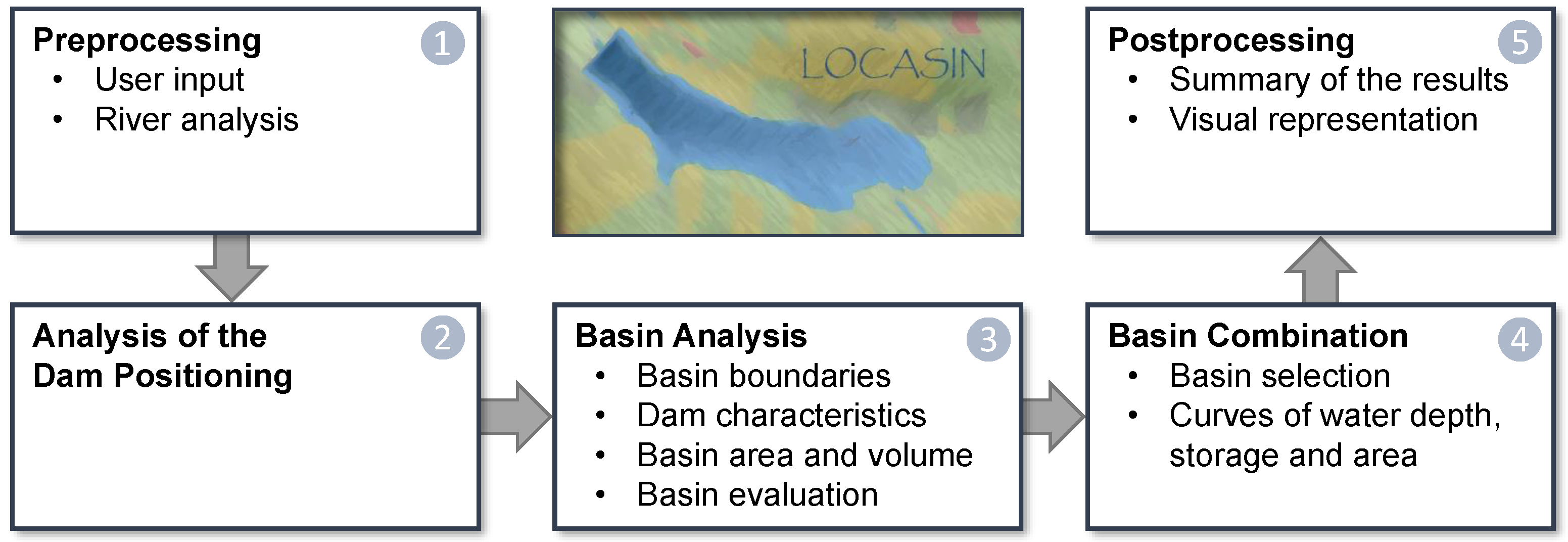
The methodology section follows the structure of the program code developed with MATLAB R2018b and comprises five parts, which are executed consecutively (Figure 1). The preprocessing result is a list of all candidate dam sites (Figure 1, Step 1). The sites are analyzed with respect to the dam positioning (Figure 1, Step 2) and the basin characteristics (Figure 1, Step 3). If sites are inappropriate for the defined criteria, they are excluded for further analyses and assigned to a specific exit code (

Table 1. Exit codes and definitions; exit codes > 0: excluded sites, exit codes ≤ 0: considered sites.

fun_1_river_analysis.m
1	river point is too close to the grid border or excluded by user defined spatial data for dam restrictions
2	river point is excluded by user defined spatial data for basin restrictions (e.g., land use)
3	target basin volume is too small for the target specific volume (=too large rivers are excluded)
4	target basin volume is too large for the target specific volume (=too small rivers are excluded)
fun_2_determine_shortest_dam.m
5	river point is excluded for further analysis, because a potential dam exists within a predefined distance
6	no possible dam orientation available to close the valley (with the defined dam length)
−1	dam height had to be reduced to close the valley (with the defined dam length)
fun_3_determine_river_points_in_basin.m
7	no basin endpoint exists (river point) for the minimum dam height
−2	dam height had to be reduced, because the basin endpoint could be found within the extent of the DEM
fun_5_determine_basin_area_and_volume.m
8	no upstream river point available for the basin area analysis
9	no basin due to an erroneous dam orientation
10	basin area touches the borders (usually occurs, if the dam does not close the valley totally)
−3	dam height had to be reduced, because the basin touched the borders of the DEM
fun_6_evaluate_basins.m
11	points of the dam axis or the whole dam are higher than the defined maximum dam height
12	maximum dam height smaller than the defined minimum dam height (dam_height_min)
13	dam axis is longer than the defined maximum dam length (dam_length_max)
14	basin volumes smaller than the defined minimum basin volume (basin_volume_min)
15	basin volumes larger than the defined maximum basin volume (basin_volume_max)
16	specific volume of the basin is smaller than the defined minimum specific volume (sV_min)
17	specific volume of the basin is larger than the defined maximum specific volume (sV_max)
18	too many exclusion-cells in the basin

) to allow for the plausibility check of the procedure. The resulting dam sites are evaluated to automatically select a reasonable combination of basins (Figure 1, Step 4) and provide a description of the relations between water depth, storage and area. The postprocessing step includes a summary and a visual representation of the results (Figure 1, Step 5). Several examples following these five steps are provided in the case study (Section 4) and the tutorial in Appendix B.

2.1. Preprocessing

The required data for the analysis of candidate dam sites are defined and imported in the preprocessing step. The user input (Section 2.1.1) describes the input data, the dam and the basin characteristics. The data are imported, structured and analyzed in the river analysis function (Section 2.1.2).

2.1.1. User Input

The user input contains mandatory and optional spatial input data (

Table 2. Required and optional spatial input data.

Structure Array	Field	Definition
grids_required.	dem	digital elevation model
	dir	flow directions
	acc	flow accumulation sum
	dem_fill	pit-filled DEM (optional)
	x_range / y_range	coordinate area to be analyzed
info_exclude_dam.(field).	name	file name of spatial data to evaluate dam locations
	exclude	array with numbers, which are excluded (all others are included)
	include	array with numbers, which are included (all others are excluded)
info_exclude_basin.(field).	name	file name of spatial data to evaluate dam and basin locations
	exclude	array with numbers, which are excluded (all others are included)
	exclude_threshold	threshold value for the maximum number of cells of one exclude group in one basin (several groups and thresholds can be defined to distinguish between different factors, e.g., settlements and forest)
	include	array with numbers, which are included (all others are excluded)
	well_suited	array with numbers, which are well suited for basin locations
	not_suited	array with numbers, which not suited for basin locations

) and parameters to define the dam and basin characteristics and saving and plotting options (

Table 3. Parameters to define dam and basin characteristics, and running, saving and plotting options.

Variable Name	Definition
dam_height_max	maximum dam height ($\mathrm{m}$, whole dam)
dam_height_min	minimum dam height ($\mathrm{m}$, at the highest position)
dam_height_buffer	dam height buffer value for the exclusion of dams ($\mathrm{m}$)
dam_length_max	maximum length of the dam axis ($\mathrm{m}$)
exclude_longer_dams	definition if the dam length is a restriction parameter (yes/no: 1/0)
basin_volume_max	maximum storage volume of the basin (${\mathrm{m}}^3$)
basin_volume_min	minimum storage volume of the basin (${\mathrm{m}}^3$)
sV_min	minimum specific volume ($\mathrm{m}\mathrm{m}$, optional parameter)
sV_max	maximum specific volume ($\mathrm{m}\mathrm{m}$, optional parameter)
dam_slope_m	slope angle: horizontal length m per 1 $\mathrm{m}$ height difference
dam_crest_width	width of the dam crest ($\mathrm{m}$)
thresh	threshold for the accumulation grid to define rivers (optional if sV_max is defined)
limit_dam_height	dam_height_max is (1): valid for the whole dam; (2): only valid for the dam axis
dam_dist_eval	evaluation step size between dam_height_min and dam_height_max ($\mathrm{m}$)
discretization_number	discretization of the curves for impounding heights, storage volumes and basin areas (number of points)
neighbors_exclude _distance	distance in which neighboring river points are excluded for further analysis after a dam location has been determined ($\mathrm{m}$)
w1_damVolume_per _basinVolume	weighting factor for criterion 1 (dam volume per basin volume)
w2_basinArea_per _basinVolume	weighting factor for criterion 2 (basin area per basin volume)
w3_share_well_suited	weighting factor for criterion 3 (share of well-suited cells)
w4_share_not_suited	weighting factor for criterion 4 (share of not-suited cells)
debug_on	debugging option to assess the analysis process (activate = 1, deactivate = 2)
save_memory	definition if inappropriate dam sites are deleted immediately to reduce main memory requirements (yes/no: 1/0)
save_grids	input grids (yes/no: 1/0, Table 4)
save_river_points	general information on all analyzed river points (yes/no: 1/0, Table 4)
save_dam_points	information on all suitable basin locations (yes/no: 1/0, Table 4)
save_basins_selected	detailed information on the selected basin combination (yes/no: 1/0, Table 4)
save_basins_as_ascii	ascii raster file for all sites with dam heights and water depths (yes/no: 1/0)
save_curves_as_excel	excel-file with basin characteristics and depth-storage-area-curves (yes/no: 1/0)
plot_exitcodes	plot with spatial distribution of exit codes (yes/no: 1/0, Table 1)
plot_spatial_overview	plot with spatial distribution of basins and dams (yes/no: 1/0)
plot_factsheet_p1	fact sheet, page 1: basin characteristics (yes/no: 1/0)
plot_factsheet_p2	fact sheet, page 2: characteristics of all dam heights of one site (yes/no: 1/0)
plot_dam_comparison	plot second page of the fact sheet for multiple sites (yes/no: 1/0)
plot_curve_comparison	plot water depth-storage-area-curves for multiple sites (yes/no: 1/0)
plot_visibility	define whether the plot is visible during plotting (visible/only saving: 1/0)
raster_selected.name	name of the background raster for the spatial plots (name from Table 2)
raster_selected.legend	description of the raster ids in ascending order
raster_selected.color	RGB-codes (0-1) of the raster ids in ascending order (one color per line)

).

The spatial input data are imported from ascii raster files and have to have the same extent and resolution. The required grids are essential for the topographic analysis of potential dam and basin sites, while the optional grids are used to evaluate dam and basin sites and can be defined flexibly. The parameters in Table 3 comprise the limits for the dam and basin dimensions; the characteristics of the dam geometry; the level of detail of the basin analyses; the weighting factors of the objective function; and debug, save and plotting options. Accordingly, they are decisive for the characteristics of the basin sites. A more detailed description of the input data is presented in Section 3.2.

2.1.2. River Analysis

In the river analysis section, the mandatory input data are imported and analyzed to define river cells based on the flow accumulation grid and the predefined threshold value thresh. The resulting river points are characterized with regard to their IDs, locations, elevation levels, upstream and downstream neighboring river point IDs and the exit codes (Table 1). The required data for this analysis are the DEM and the flow direction grid. Finally, the river points are evaluated with respect to their locations. That implies that river points which are too close to the borders or which are located in restricted areas (e.g., within settlements) are excluded from the potential dam sites and the following analyses.

2.2. Analysis of the Dam Positioning

The evaluation of the best dam axis orientation in the valley is performed for all potential dam sites separately. The DEM is clipped for the analyses with respect to the river point and the predefined maximum dam length to save computational costs. The procedure to determine the dam positioning is based on three criteria:

• The dam axis has to be an almost straight line through the respective river point.
• The orientation of the dam axis has to be the shortest waylength to close the valley.
• The elevation at the boundaries of the clipped DEM in extension of the dam axis has to be above the dam crest.

The bases for the analysis are multiple generated raster datasets, which are intersected in order to establish potential dam orientations. These include the distance of any raster cell to the river point, the angles of the line to the river point in horizontal and vertical directions and a separation of the cells in the east and west to guarantee a positioning of the dam endpoints at opposing sides of the river point. Furthermore, the shoreline for the potential water level is determined and evaluated regarding the elevation in extension of the dam. The selected final dam axis is the shortest linkage of two points on the shoreline, which fulfills the conditions of the angles, and thus, defines a straight line through the river point.

The shoreline is defined by the potential maximum dam height. If no possible dam axis can be determined, an iterative extension of the clipped DEM is performed, which is followed by a consecutive reduction of the dam height by the distance until a dam axis is found or the minimum dam height is reached. Thus, both variables largely influence the computational power needed. A reduction of the computation time can be achieved through an increase of the variable neighbors_exclude_distance, which results in the exclusion of neighboring river points of a dam location within a specific distance.

2.3. Basin Analysis

The analysis of potential basins is performed consecutively for all possible dam locations and is separated in four steps. If a site does not fulfill the predefined criteria, it is excluded after the respective step (Table 1).

2.3.1. Basin Boundaries

The purpose of the first step is to determine the approximate extent of a potential basin area, which is necessary to clip the DEM, and consequently, to reduce the main memory requirements of the following steps. The extent is estimated by including all points, which may be within the basin. These comprise all upstream neighbors of the dam river point with an elevation below the dam crest elevation. Additionally, the endpoints of potential dams at these neighboring points are considered. It may happen that no river points having an elevation above the dam crest can be found within the total extent of the analyzed DEM. In this case, the dam crest elevation is set to the elevation of the highest upstream neighbor, where the resulting dam height needs to be within the predefined range.

2.3.2. Dam Characteristics

The dam characteristics and its geometry are decisive for the economical evaluation of a basin, and thus, are considered in detail. The geometry of the dams is described by four parameters: the elevation of the dam crest, the dam axis orientation (Section 2.2), the width of the dam crest and the dam slopes perpendicular to the dam axis. The elevation of the dam crest is defined by the river point elevation and the maximum dam height, which may have been reduced from the predefined value in Section 2.3.1.

The basis to build the dam surface is the dam axis orientation. In a first step, the line representing the dam axis is extrapolated to the borders of the clipped basin-DEM (Section 2.3.1). Next, the dam is widened and the surface elevation is recorded for every point on the dam for the predefined potential dam heights (steps from dam_height_max to dam_height_min by distances of dam_dist_eval). The result represents the surface elevations of dams with different maximum heights. The final dam geometry is obtained by subtracting the dam surface and the DEM. Every potential dam is described by its height, its volume and its dam axis length.

2.3.3. Basin Area and Volume

The potential efficiency of a basin is usually evaluated with respect to its storage volume. The determination of the basin volume and area is the final step in the description of a potential dam site. The analysis is based on the intersection of the clipped DEM (Section 2.3.1) and the surface elevations for all potential dam heights (Section 2.3.2), resulting in the shorelines of potential basins. The basin area of the maximum dam height is determined with a river point upstream of the dam point. This point lies within the respective shoreline, and thus, defines which side of the shoreline is water. As a consequence, the inundation areas for the smaller dam heights equal the reduced maximum basin area based on the DEM-surface elevation-intersection. The flooded areas and the respective storage volumes are calculated for all potential dam heights. The storage volume is additionally determined for a wall geometry of the dam to quantify the storage volume that is lost due to the slopes of a realistic dam geometry.

2.3.4. Basin Evaluation

The last step of the basin analysis is an evaluation of all potential dam heights and the respective basins for each site. The selection of the best dam for a respective site is based on user-defined weighting factors. At the beginning of the evaluation, the potential dam heights are checked with regard to predefined criteria. These include the ranges of the dam height, the dam length, the basin volume and the specific volume. Furthermore, the number of restricted cells in the flooded area is determined and compared to its respective threshold values. If all potential dam heights are excluded, the site is rejected. The selection of the ideal dam height is based on an objective function (Equation (2)), which includes four criteria to compare the dam and basin characteristics with one another:

• Criterion 1: dam volume per basin volume (m${}^3$/m${}^3$).
• Criterion 2: basin area per basin volume (1/m).
• Criterion 3: share of well-suited cells in the basin area (−) (Section 3.2).
• Criterion 4: share of not-suited cells in the basin area (−) (Section 3.2).

In order to combine the criteria, a scaling of the individual criteria between zero and one is performed, where the optimum of the resulting dimensionless parameters $C_1$ to $C_4$ is one.

$$C_x=\left\{\begin{array}{}\mathrm{(1a)}& 1-\frac{\mathrm{criterion}x-min\left(\mathrm{criterion}x\right)}{max\left(\mathrm{criterion}x\right)-min\left(\mathrm{criterion}x\right)},\hfill & \mathrm{where}x=1,2,4\hfill \mathrm{(1b)}& \frac{\mathrm{criterion}x-min\left(\mathrm{criterion}x\right)}{max\left(\mathrm{criterion}x\right)-min\left(\mathrm{criterion}x\right)},\hfill & \mathrm{where}x=3\hfill \end{array}\right.$$

The respective weighting factors are defined by the user (Section 3.2). The factors $w_1$ to $w_4$ are adapted to ensure that their sum equals one. Thus, the value of the objective function f ranges between zero and one with its optimum at the upper limit.

$$f=w_1\times C_1+w_2\times C_2+w_3\times C_3+w_4\times C_4$$

(2)

The optimum dam height of every site is characterized by the maximum value of the objective function. It is picked for the following selection procedure.

2.4. Basin Combination

The resulting basins from the previous analysis include all potential dam sites. However, the dam and basin areas of the different sites are overlapping, which implies that not all of them can be included in the same basin combination. Thus, an assorting of the basins is required based on their suitability.

2.4.1. Basin Selection

The selection of the basin combination is based on the same objective function and criteria which were described in Section 2.3.4. The scaling procedure of the four criteria to determine the parameters $C_1$ to $C_4$ comprises the best dam heights of all possible dam locations. The basins of the final combination are chosen in an iterative procedure: The first basin is the one with the largest objective function value. Consequently, all overlapping basins are deleted from the database, which brings the second-best basin to the top of the list. Again, this basin is chosen and overlapping basins are deleted, and so forth. The final result is a combination of basins which do not interfere with one another.

2.4.2. Curves of the Basin Depth, Volume and Area

The characteristics of a basin depend on the relationship between water depth, storage volume and flooded area. Hence, the respective curves are determined for the dam geometry and for the wall geometry. The number of sampling points is defined by the variable discretization_number. The results can be used, e.g., as input data for estimating the efficiency of a basin with a hydrological model [10].

2.5. Postprocessing

The postprocessing section includes the summary, storage and visual representation of the results.

2.5.1. Summary of the Results

The results contain information about the analysis process, the characteristics of all possible dam sites and the dams of the selected combination. The required level of detail depends on further planned applications; e.g., the visualization of the results (Section 2.5.2) or hydrological efficiency estimations of basin combinations. A detailed description of the output data is given in Section 3.3.

2.5.2. Visual Representation

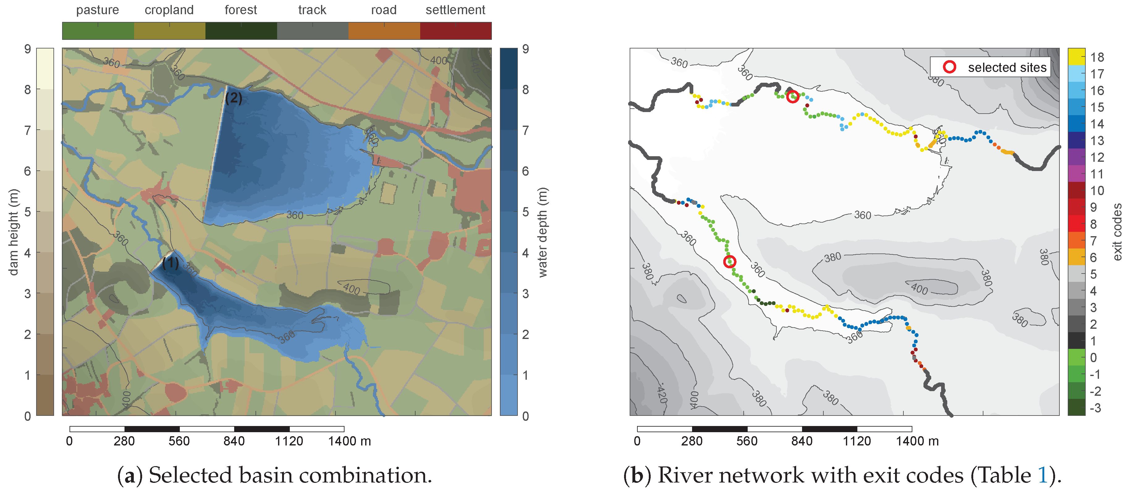
The summarized output data can be analyzed and visualized in multiple ways. The included visual representation comprises six figures: 1 and 2 give an overview on the results (Figure 2a) and the sorting procedure (Figure 2b). 3 and 4 characterize the single basins on a double-sided fact sheet (Figure 3). 5 and 6 allow one to compare the dam sites (not shown). The figures are taken from one of the examples of the case study.

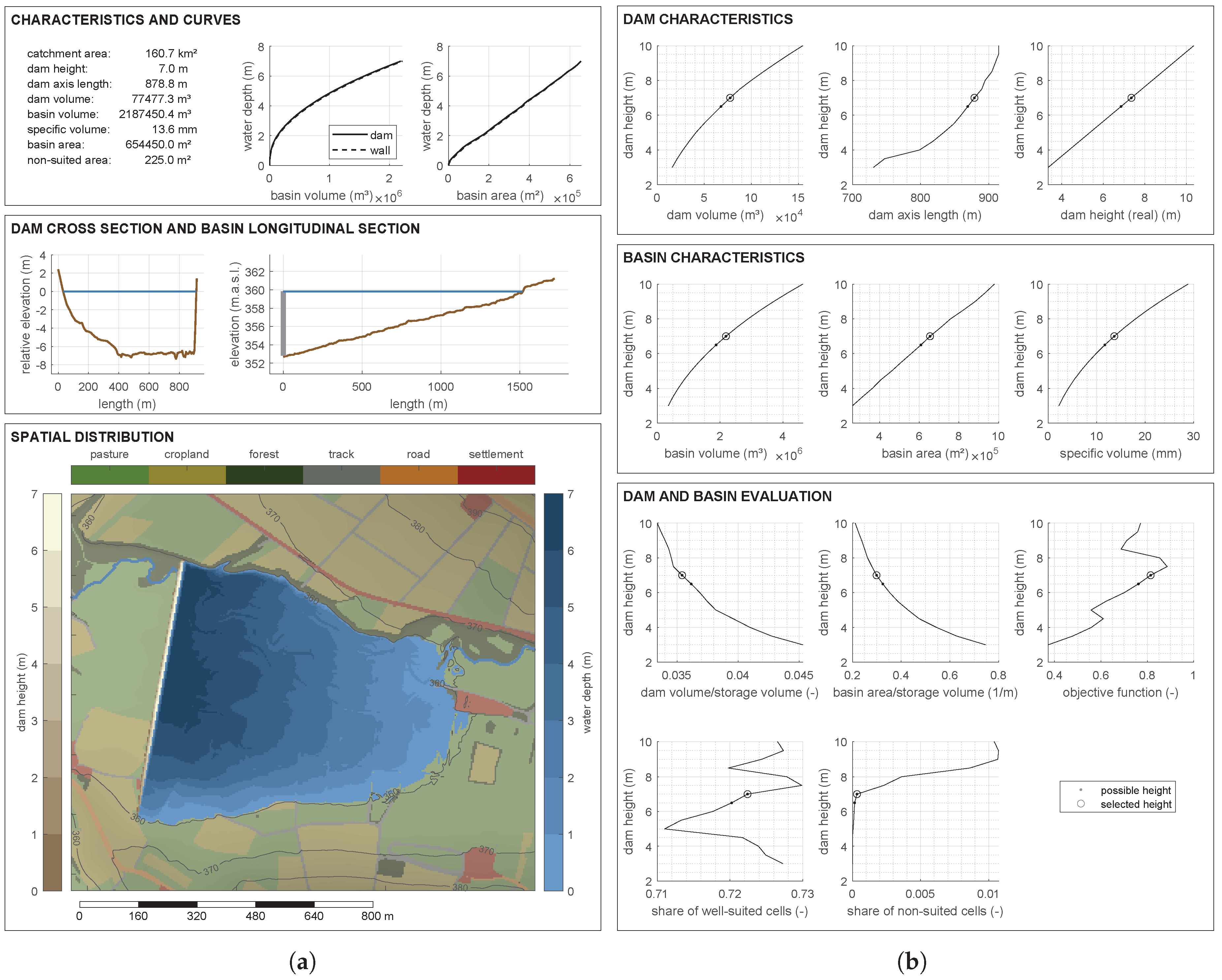
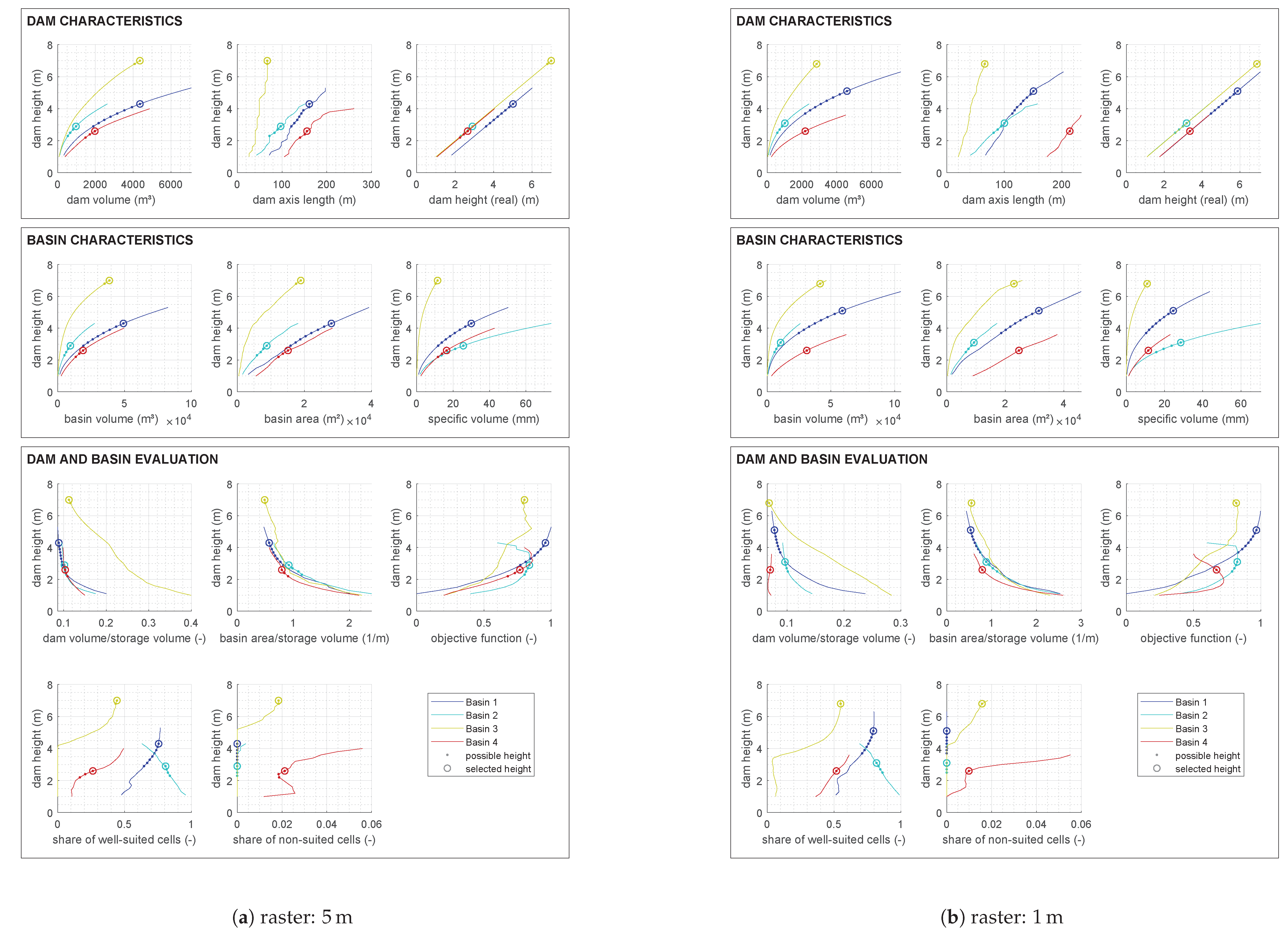
While the first page of the fact sheet (Figure 3a) shows the characteristics of the basin for the selected dam height, the second page (Figure 3b) allows one to understand the selection and to examine alternatives. The variable dam height in this illustration corresponds to the dam height at the location of the river, whereas the term dam height (real) indicates the maximum dam height of the entire dam structure. The marked possible dam heights represent dam heights for which the corresponding basins meet the criteria defined by the user and thus could potentially be implemented. In this test case, for example, the maximum number of unsuitable cells within a basin area causes the maximum value of the target function not to be selected. The different curves can be used to evaluate the properties at alternative dam heights and to adjust the limits if necessary.

3. Code Structure and Data Definitions

The general procedure of the analyses is explained in Section 2, whereas the following paragraphs comprise technical aspects of the code structure and a more detailed description of the input data and output data.

3.1. Code Structure

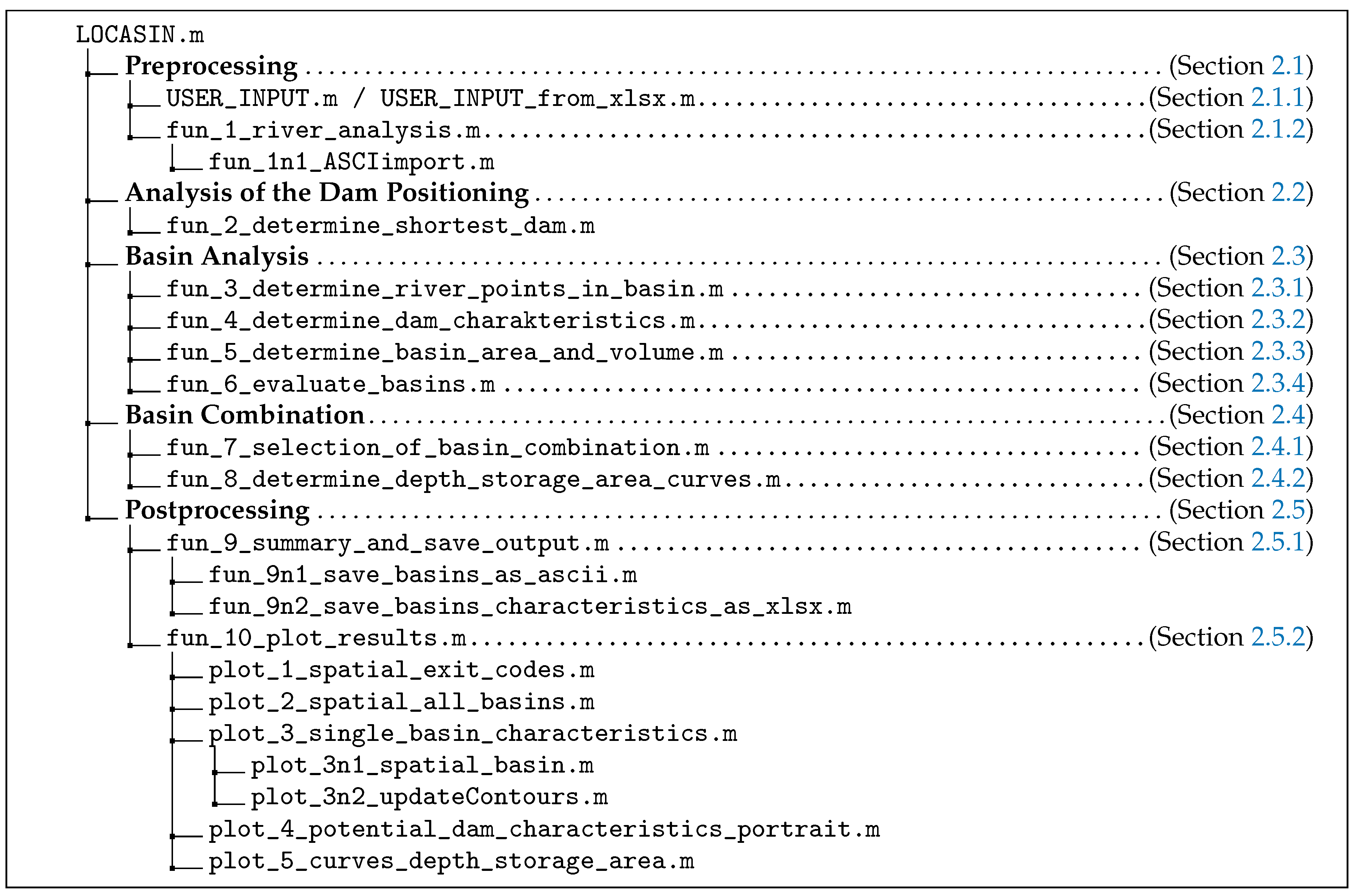
The program structure, including the single functions’ names and the references to the methodology section, is illustrated in Figure 4. The variables, which can be adapted by the user, are summarized in the function USER_INPUT.m. Alternatively, the specified data can be defined in an Excel-table, which is imported and allocated by the function USER_INPUT_from_xlsx.m. The parameters are specified in Section 3.2. They include required and optional spatial input data (Table 2) and parameters to define dam and basin characteristics and saving and plotting options. The functions listed in Figure 4 are run consecutively for each potential site. If a dam or basin with the user-defined properties is not possible at the particular location, the respective exit_code is adjusted (Table 1). Positive exit_codes lead to an exclusion of the location for further analyses, whereas negative exit_codes only indicate a reduction in the target dam height.

3.2. Input Data

The spatial input data (Table 2) is the basis for the analyses (required grids) and site evaluations (optional grids). The required grids include a digital elevation model (DEM) and grids with flow direction and flow accumulation information. The pit-filled DEM can optionally be considered for the visualization of the basin cross-section and longitudinal section. The coordinate ranges are also optional parameters, which can be defined to extract a subarea of a larger grid, and thus, reduce the main memory requirements during the actual analysis. Further optional grids can be assigned to the structure arrays info_exclude_dam and info_exclude_basin: the structure array info_exclude_dam is applied to analyze potential dam positions, whereas info_exclude_basin is used for basin and dam areas. The first parameter is used to exclude certain dam points already at the beginning of the analyses, and thus, save calculation time. The aim of the second parameter is to evaluate the influenced area of the combination of dam and basin after the analyses are completed. The field names (field) of both structure arrays are customizable (e.g., river_buffer, landuse, geology, conductivity) and thus can contain various data, allowing the input data for the evaluation of the sites to be individually selected and extended. In contrast, the second order fields (column field in Table 2) require predefined names (e.g., name, exclude, include; Table 2). These fields contain user-defined numbers, which are used to exclude specific sites or to rank the suitability of basins. Basins for which the areas that are described with the parameter exclude exceed the specified limit exclude_threshold are not considered in the results. In contrast, the ranking of the basins is based on the fields well_suited and not_suited, in which for instance land use numbers can be defined that are well suited for a basin location (e.g., grassland) or not suited for a basin location (e.g., settlement areas). e.g., the inclusion of settlement areas in the exclude and not_suited variables leads to a reduction of the corresponding factor of the objective function ($C_4$, Equation (2)). In case the value of exclude_threshold is exceeded, e.g., when having a higher dam heigth, the corresponding basin of this dam height is excluded accordingly.

The user-defined parameters in Table 3 are subdivided into seven groups. The first group describes the limits for the dam and basin extents. Potential dams or basins beyond these values are excluded. The second group defines the characteristics of the dam structure. The respective parameters do not influence the feasibility of implementing a dam site, but its (economic) suitability. The third group affects the level of detail of the basin detection procedure. The values are decisive for the number of investigated dam positions, the number of potential dam heights and the accuracy of the output curves. Thus, they affect the computational effort; i.e., computation time and main memory requirements. The fourth group are weighting factors of the objective function to favor specific basin locations (Equation (2)). The save and debug options are for analysis purposes; With the debugging-option, intermediate stages of the analyses can be plotted to understand and assess the site-selection process. The save options define the level of detail of the saved output data. The requirements are user-specific and depend on the purpose for which the results are needed. The plotting options define the way how results are visualized. The figures can also be plotted separately with the LOCASINplotting tool using already saved results. The variable raster_selected defines the background map for the spatial overview of the results.

3.3. Output Data

The most common output data configurations are summarized in

Table 4. Output data files and variables (“r”: row, “c”: column).

Variable	Definition
input_grids_used.mat
grids	required grids for the analysis (DEM)
grids_exclude	variable grids for the exclusion of dams or basins (e.g., land use)
info_exclude_dam	additional information on the grids to exclude dams
info_exclude_basin	additional information on the grids to exclude basins
river_points.mat
id	identification number of the river point
x_coord	x-coordinate in the used metric coordinate system
y_coord	y-coordinate in the used metric coordinate system
exit_code	exit codes to analyze why river points had to be excluded (Table 1)
dem	elevation of the river point
dem_fill	elevation of the river point taken from the DEM with filled sinks
acc	accumulation value of the river point
vorgaenger	upstream neighbor(s) of the river point
nachfolger	downstream neighbor of the river point
dam_points.mat | basins_selected.mat
id, x_coord, y_coord and dem as in river_points.mat
dam_top_elev	elevation of the dam crest
dam_height	maximum dam height
dam_axis_lengths	length of the dam axis
dam_volumes	dam volume (c1: whole dam, c2: waterside of the dam)
basin_volumes	maximum storage volume of the basin (cross-section type: c1: dam, c2: wall)
basin_areas	maximum flooding area of the basin (cross-section type: c1: dam, c2: wall)
dam_axis_lengths_segments	length of single segments of the dam axis to analyze the dam cross-section
dam_axis_heights	dam heights for the single segments of the dam axis
refGK_dam_coords	coordinates of all dam points including the crest and the slopes in metric coordinate system (row 1: x-coordinates, row 2: y-coordinates)
dam_heights	heights of all dam points including the crest and the slopes
dam_elevation	elevations of all dam points including the crest and the slopes
refGK_BASIN_x	x-coordinates of the basin raster data
refGK_BASIN_y	y-coordinates of the basin raster data
refBASIN_depth_dam_cross.	basin raster data with water depth for a dam cross-section
refBASIN_depth_wall_cross.	basin raster data with water depth for a wall cross-section
ShA_dam	curves of basin storage, water depth and basin area (dam cross-section)
ShA_wall	curves of basin storage, water depth and basin area (wall cross-section)
crit1_damvol_per_storage	criterion 1: dam volume per basin storage volume (Section 2.3.4)
crit2_area_per_storage	criterion 2: basin area per basin storage volume (Section 2.3.4)
crit3_share_wellsuited_c.	criterion 3: share of well-suited cells in the basin (Section 2.3.4)
crit4_share_notsuited_c.	criterion 4: share of not-suited cells in the basin (Section 2.3.4)
objective_function	result of the objective function (for basins_selected.mat)
curve_potential_dam_basin	dam and basin characteristics for all possible potential dam heights (rows: potential dam heights; c1: evaluated dam heights, c2: dam volumes, c3: dam axis lengths, c4: basin volumes, c5: basin areas, c6: specific volume, c7: objective function, c8: correspondence to user requirements (1: possible, NaN: restricted), c9: real maximum dam height, c10: criterion 1, c11: criterion 2, c12: criterion 3, c13: criterion 4, c14: number on non-suited cells)

. The variables to define the files to be saved are described in Table 3. The input grids and the user-defined exclusion information are saved in the file input_grids_used.mat, which may be required for the plotting of background maps. The file river_points.mat contains general information of all river points and enables an analysis of the reasons for the exclusion of specific river points (exit codes in Table 1).

The detailed descriptions of possible dam sites are given in the files dam_points.mat and basins_selected.mat. The latter involves the dams of the selected combination and can be used for a combined efficiency analysis. In contrast, dam_points.mat contains all possible dam sites, which have not been excluded in the previous analysis. The file can be used to characterize potential dam sites and to conduct a manual selection of basin locations.

4. Case Study

The objective of the case study is to illustrate the applicability and flexibility of LOCASIN. We selected two area extents from the Main catchment in Bavaria (Germany) with maximum accumulation areas of about 5 $\mathrm{k}$$\mathrm{m}$${}^2$ and 200 $\mathrm{k}$$\mathrm{m}$${}^2$. The different catchment sizes and valley types of the sections allow one to detect a large range of basin volumes.

4.1. Input Data and Parameters

The required file names and parameters are summarized in

Table 5. Input data and parameter selection for the case study.

Variable Name	Case 1	Case 2	Case 3	Case 4
investigation area	region 1		region 2
raster resolution	5 $\mathrm{m}$	1 $\mathrm{m}$	5 $\mathrm{m}$	1 $\mathrm{m}$
required and optional spatial input data
grids_required.x_range	[ 4,476,340 , 4,477,111 ]		[ 4,471,081 , 4,477,113 ]
grids_required.y_range	[ 5,548,272 , 5,549,619 ]		[ 5,543,462 , 5,546,414 ]
grids_required.dem	dem5.txt	dem1.txt	dem5.txt	dem1.txt
grids_required.dem_fill	demfill5.txt	demfill1.txt	demfill5.txt	demfill1.txt
grids_required.dir	dir5.txt	dir1.txt	dir5.txt	dir1.txt
grids_required.acc	acc5.txt	acc1.txt	acc5.txt	acc1.txt
info_exclude_dam.river_buffer.name	buffer5.txt	buffer1.txt	buffer5.txt	buffer1.txt
info_exclude_dam.river_buffer.include	70
info_exclude_basin.landuse.name	use5.txt	use.txt	use5.txt	use.txt
info_exclude_basin.landuse.exclude{1}	[5 , 6]
info_(...).landuse.exclude_threshold{1}	1000
info_exclude_basin.landuse.well_suited	1
info_exclude_basin.landuse.not_suited	[5 , 6]
parameters to define dam and basin characteristics
dam_height_max	7		10
dam_height_min	1		3
dam_height_buffer	0.05
dam_length_max	100		500
exclude_longer_dams	0
basin_volume_max	60,000		4,000,000
basin_volume_min	5000		800,000
sV_max	30
sV_min	10
dam_slope_m	2
dam_crest_width	3
thresh	[ ]
limit_dam_height	1
dam_dist_eval	0.2		0.5
discretization_number	41
neighbors_exclude_distance	4		24
w1_damVolume_per_basinVolume	0.3
w2_basinArea_per_basinVolume	0.3
w3_share_well_suited	0.2
w4_share_not_suited	0.2
run, save and plotting options (identical for Case 1 to Case 4)
debug_on	0	plot_visibility		0
save_memory	1
save_grids	1	plot_exitcodes		1
save_river_points	1	plot_spatial_overview		1
save_dam_points	0	plot_factsheet_p1		1
save_basins_selected	1	plot_factsheet_p2		1
save_basins_as_ascii	1	plot_dam_comparison		1
save_curves_as_excel	1	plot_curve_comparison		1

. The four cases differ in terms of the spatial extent (region 1, region 2), raster resolution (1 m, 5 m) and specific dam and basin characteristics.

We defined two raster files to include or exclude potential dam sites. The raster river_buffer defines an area of 70 $\mathrm{m}$ along the real river network; potential dam points outside this range are excluded. The second raster contains land use information, which is used to exclude dam sites and to evaluate the suitability of the basins. Basins containing more than 1000 $\mathrm{m}$${}^2$ of the land use classes 5 (large roads) or 6 (settlements) are excluded. The shares of well suited cells (1: grassland) and not suited cells are considered in the objective function for the dam and basin evaluation. The parameter to define the dam and basin characteristics differs in the ranges of dam heights and basin volumes. Furthermore, the level of detail varies with regard to the respective computational effort. The run and save options are identical. The threshold value is left empty and in is consequently defined based on the minimum basin volume and the maximum specific volume.

4.2. Performance Evaluation

The applicability of LOCASIN is flexible with regard to the input data and the raster resolution, the level of detail of the results and the computational effort. The results of the four cases and their visualization are described in Section 4.3.

Table 6. Evaluation extent and computation time of the four cases.

Parameter	Case 1	Case 2	Case 3	Case 4
evaluation extent
raster size (cells)	4.2 × 104	1.6 × 106	7.1 × 105	1.7 × 107
potential sites	653	4408	2660	15546
analyzed sites	361	418	420	930
possible sites	147	148	56	68
selected sites	4	4	2	2
computation time ($\min$)
preprocessing	0.847	1.817	0.951	2.455
dam analysis	0.038	0.313	0.138	5.620
basin analysis	0.210	3.954	1.289	32.327
combination selection	0.001	0.007	0.003	0.049
saving results	0.011	0.087	0.578	0.511
plotting results	0.074	2.182	1.374	24.860
total duration	2.022	8.547	4.505	66.012

gives an overview over the evaluation extents, i.e., the raster size and number of river points, and the resulting computational effort of the four cases (Intel(R) Xeon(R) CPU E3-1270 V2 at 3.50GHz, 32.0 GB RAM). While there is only a relatively small difference with regard to the raster resolution among case 1 and case 2 (factor: 4.2), the computation time of the basin analysis increases significantly by a factor of about 14.7 from case 3 to case 4. In consequence, the required level of detail may be adjusted to obtain a reasonable computational effort.

4.3. Results and Visualization

The visualization of the results provides a basis for a plausibility check and an evaluation of the results. It includes six figures:

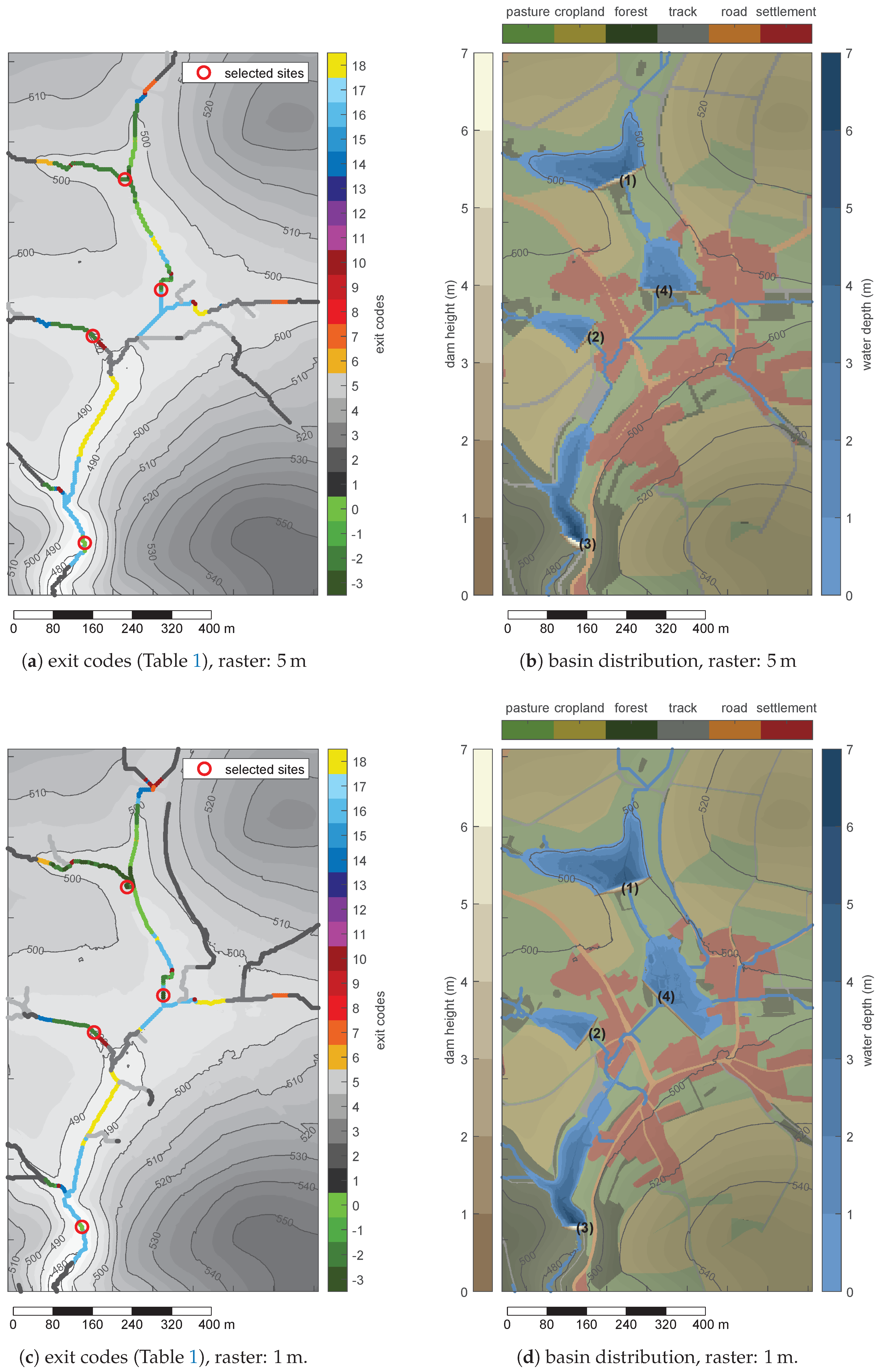
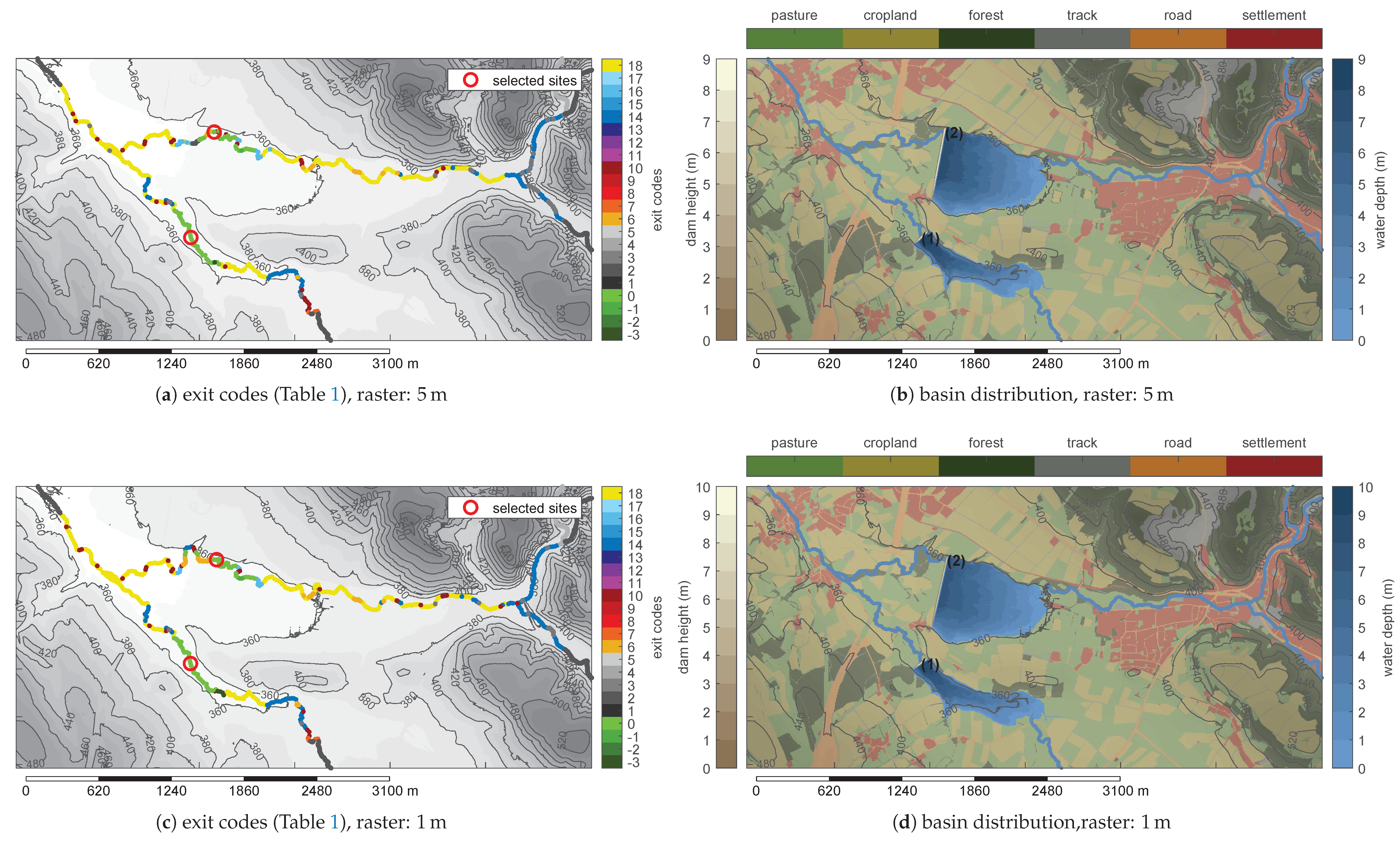
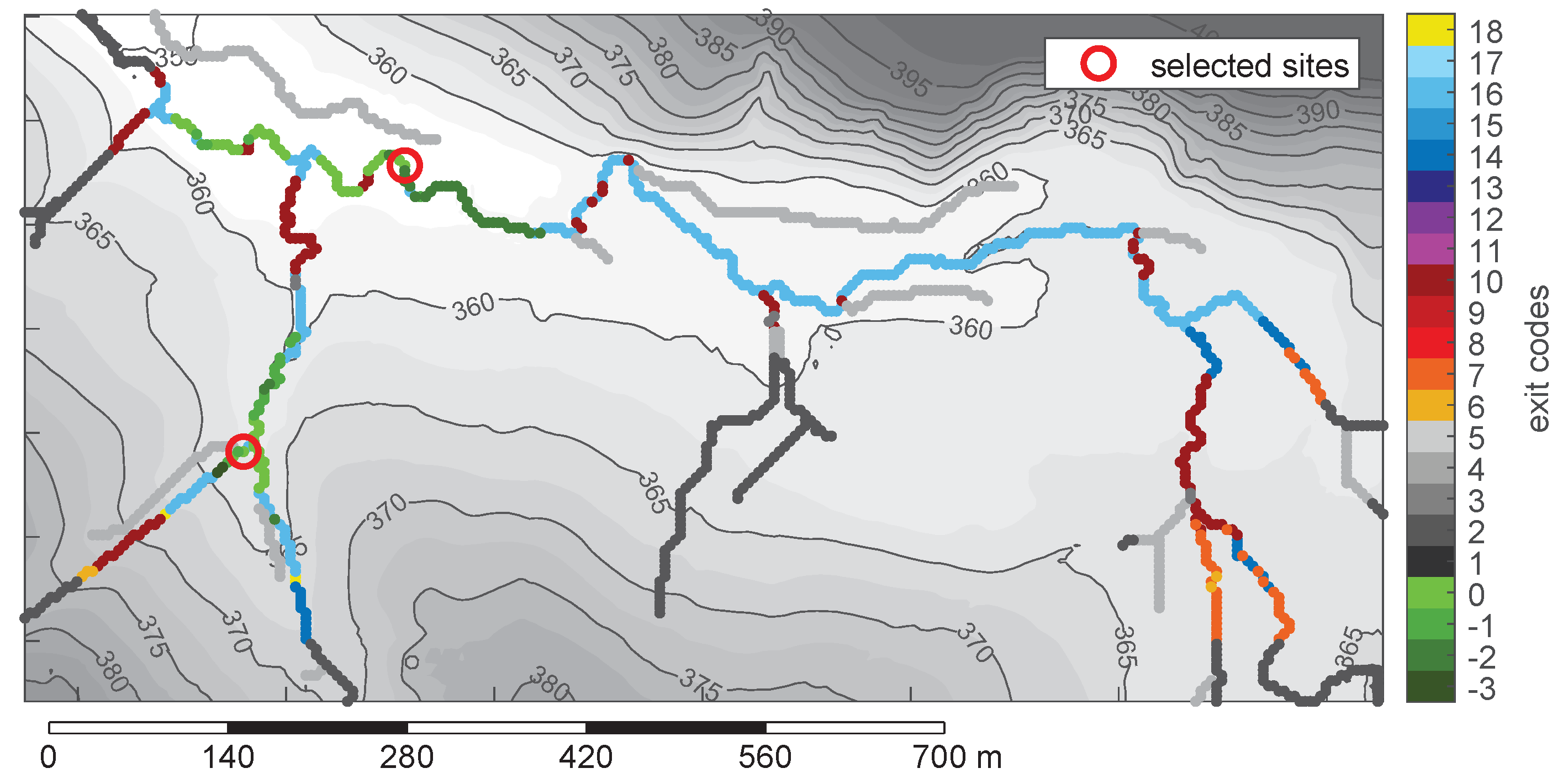
• The spatial distribution of the river points is plotted with different colors for the exit codes (Table 1). Individual raster data (e.g., DEM) can be displayed as a background map. The purpose of the figure is to analyze the plausibility of the results and the sorting procedure (Figure A1a,c and Figure A7a,c).
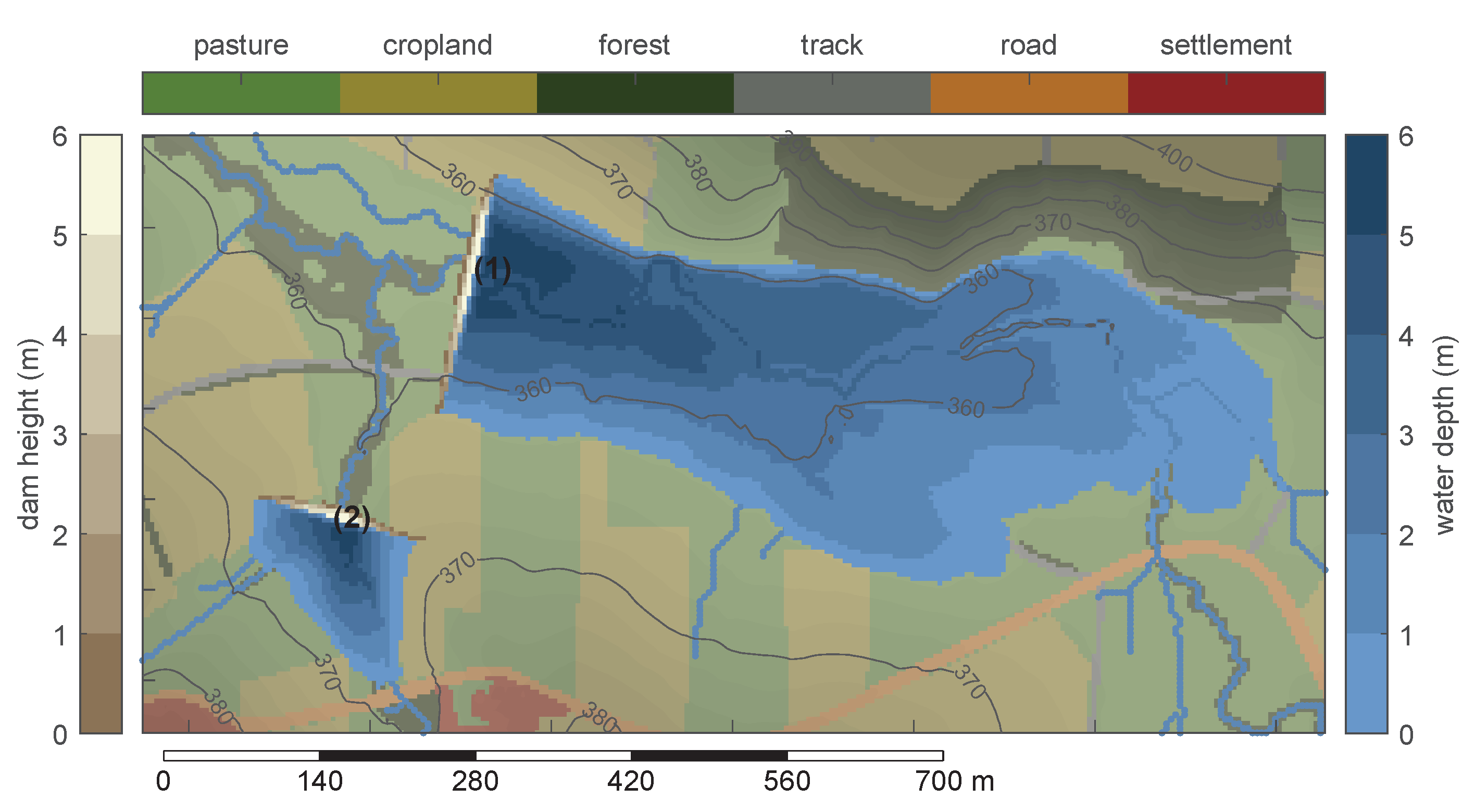
• The selected basin combination is displayed to give an overview of the final results. It includes the basin number, the dam orientation with the respective dam heights and the basin area with distributed water depths. The background map includes the DEM, an individual map (e.g., landuse) and the river network (Figure A1b,d and Figure A7b,d).
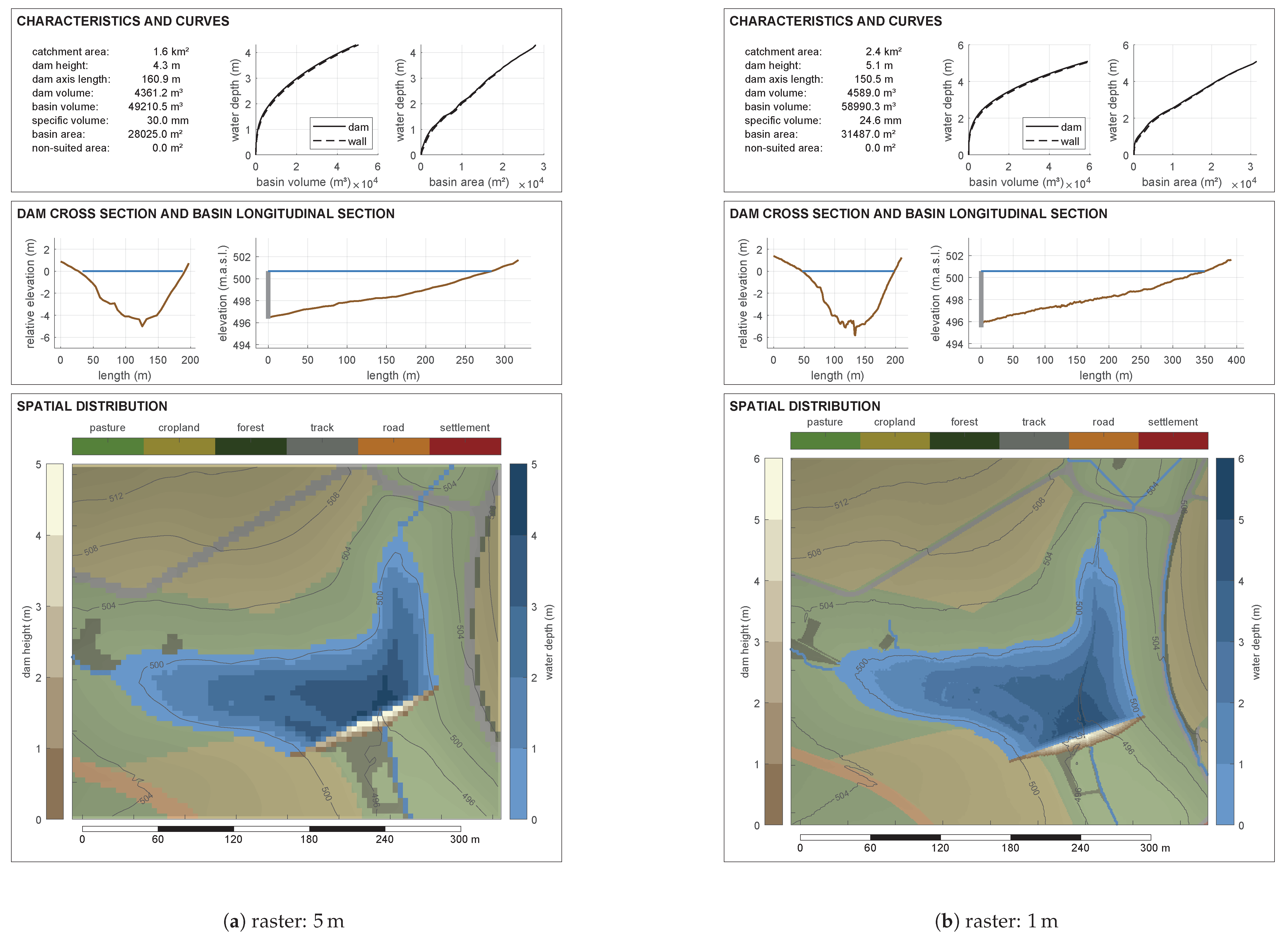
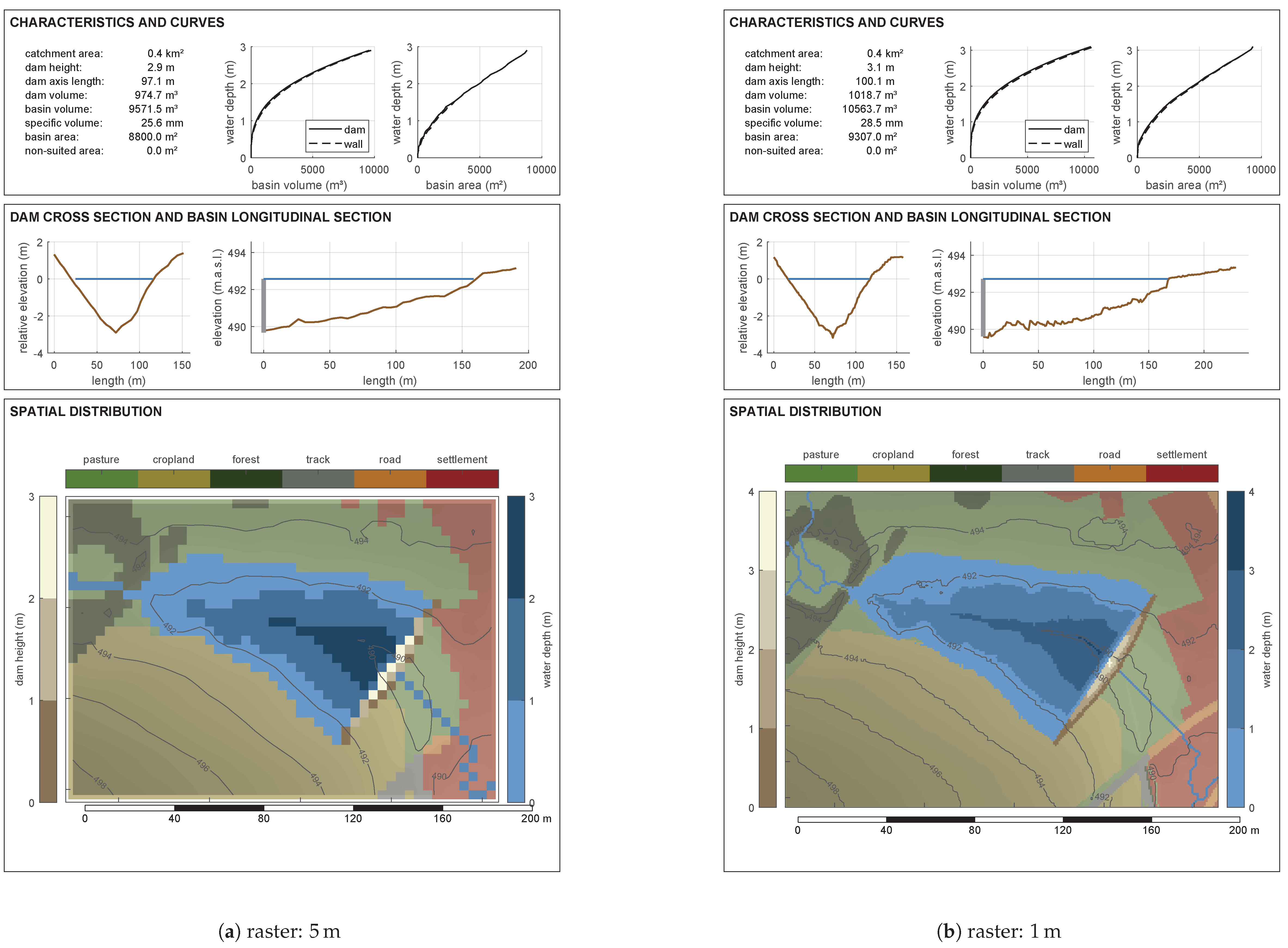
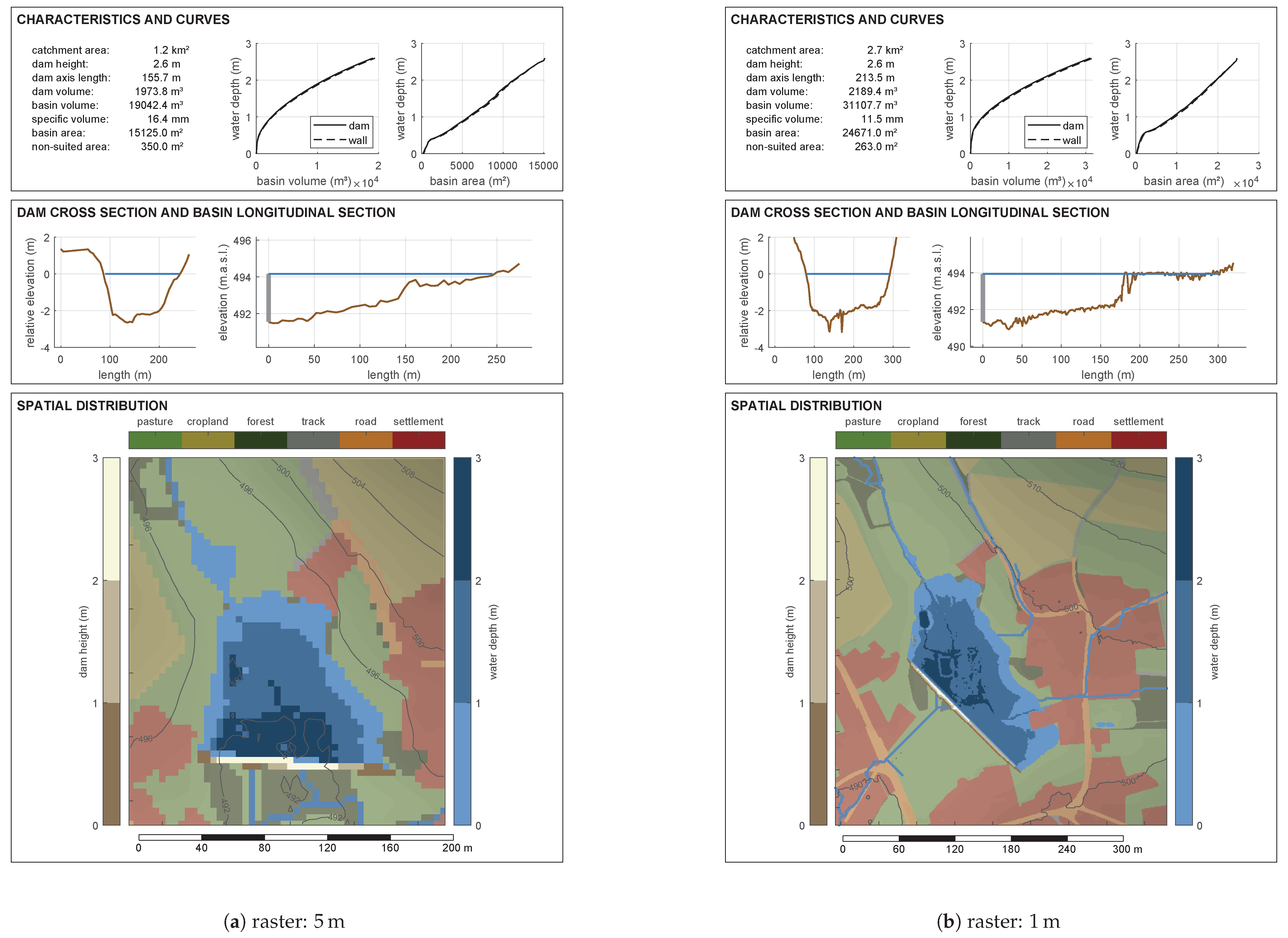
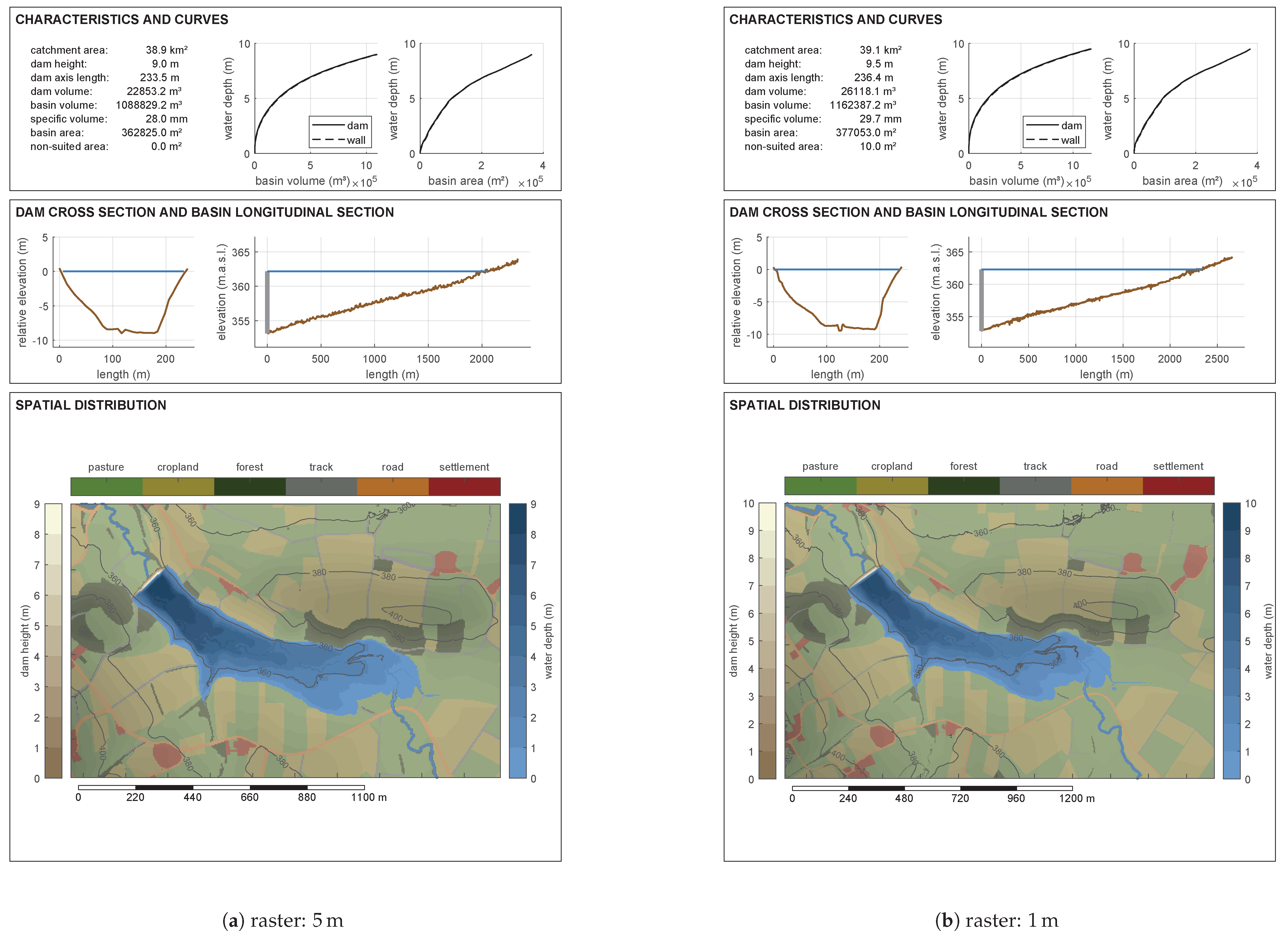
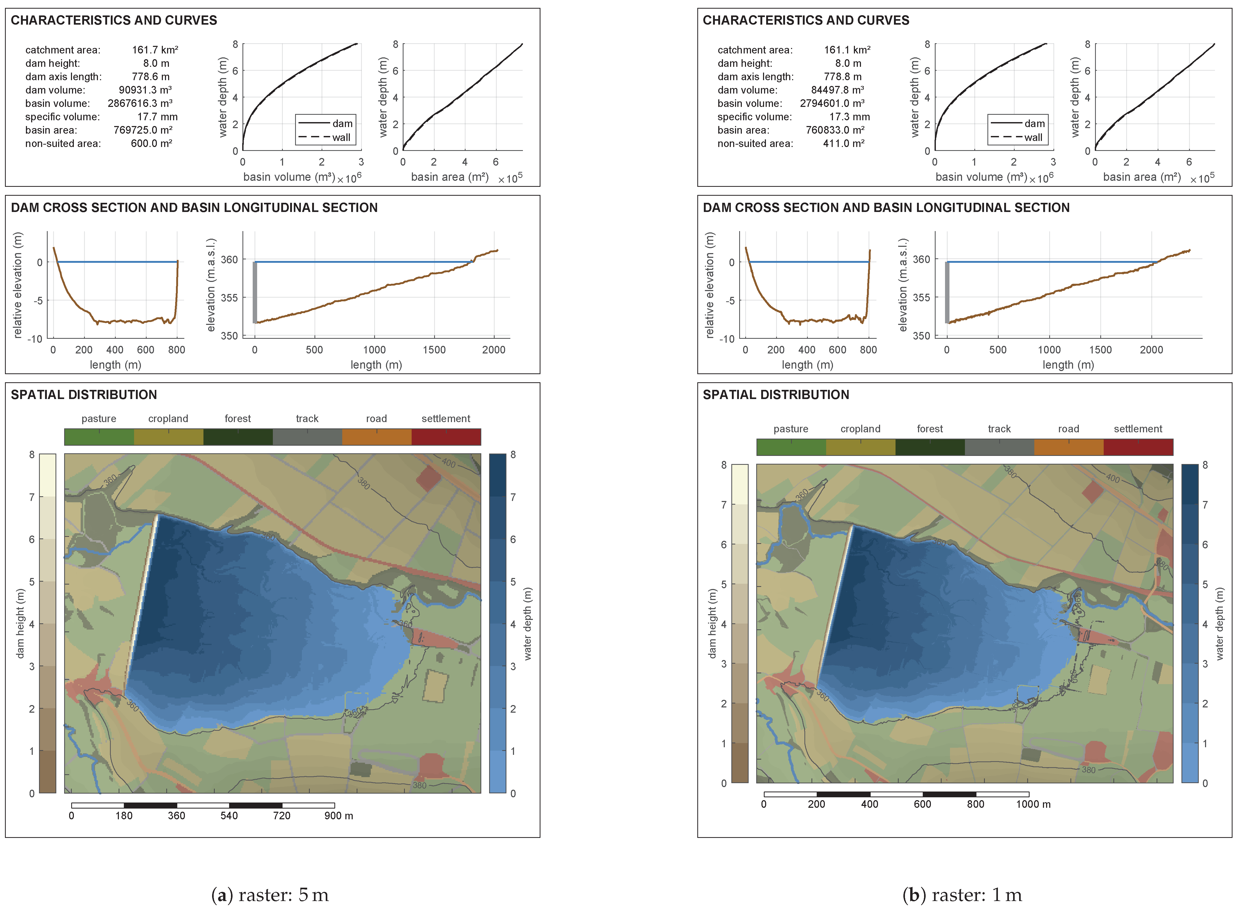
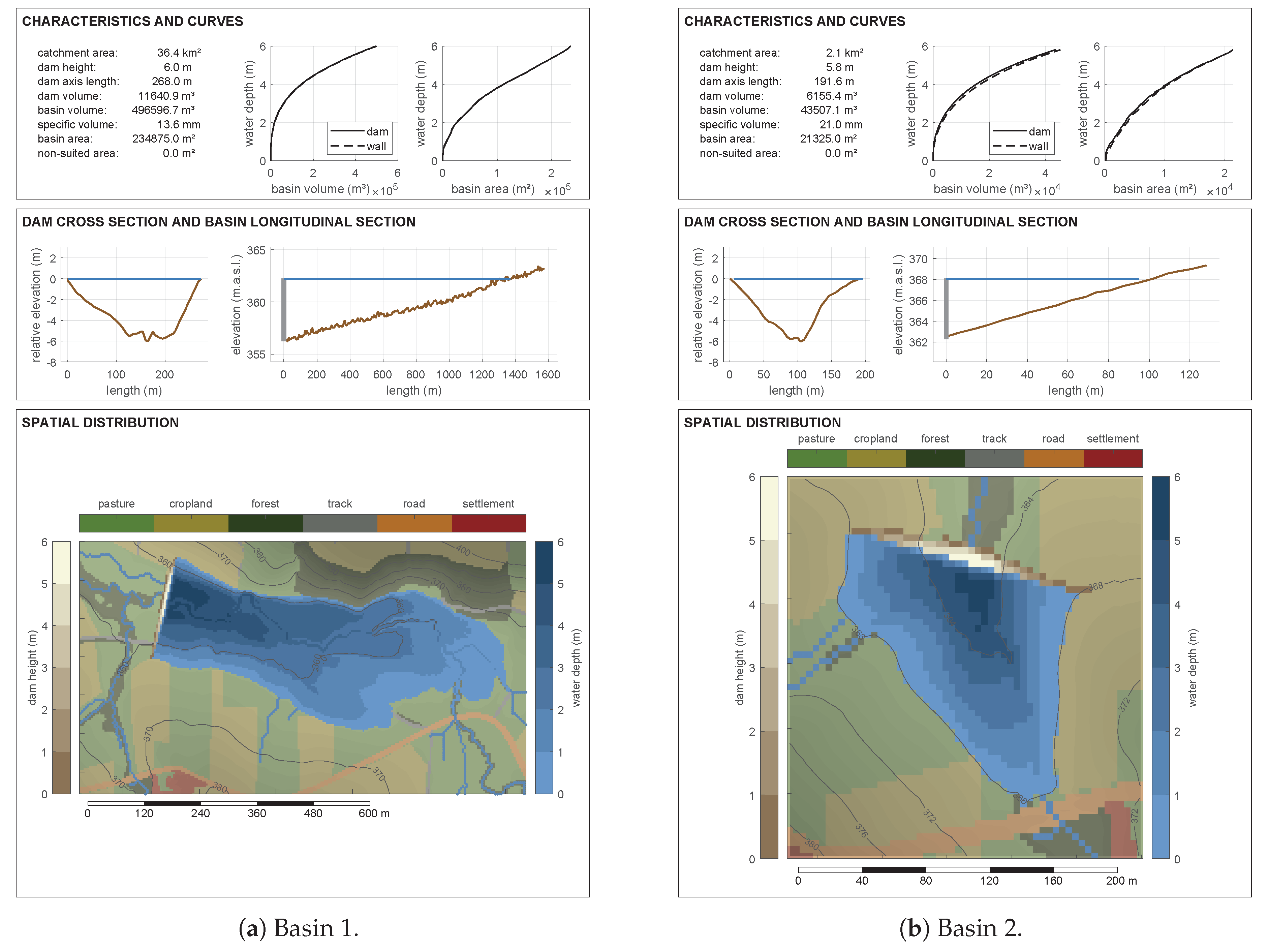
• The characterization of the single basins is summarized on a double-sided fact sheet. The first page includes general information on the selected basin; curves of the water depths, the storage volume and the flooding area; the dam’s cross-section; the basin longitudinal section; and a top view of the basin (Figure A3, Figure A4, Figure A5, Figure A6, Figure A9 and Figure A10).
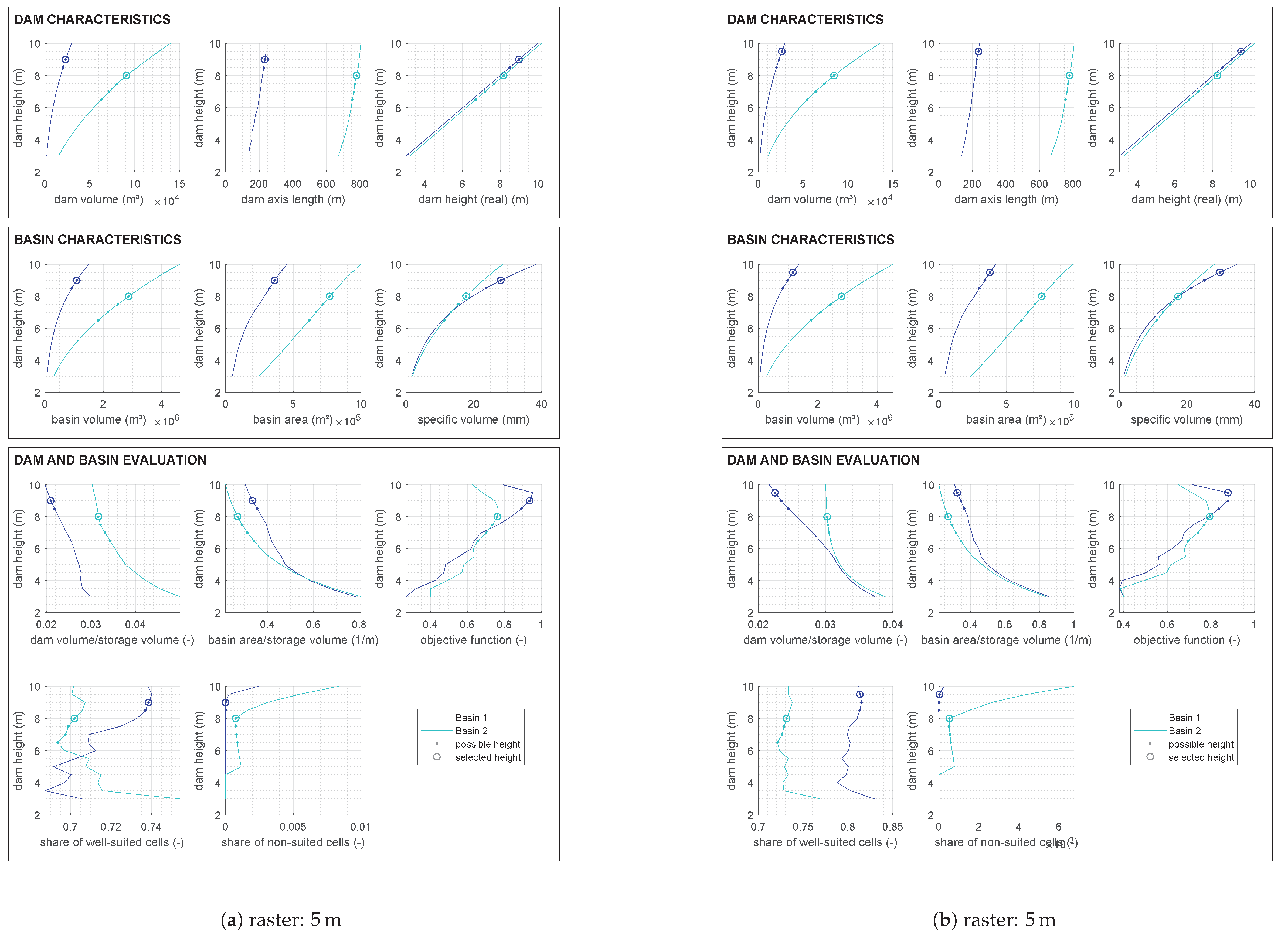
• The second page displays information on all potential dam heights; i.e., the dam characteristics, the basin characteristics and the dam and basin evaluation criteria.
• The curve of water depth, basin volume and basin area is decisive for the efficiency estimation and the influencing area of a basin. It is, thus, included on the first page of the fact sheet, but can additionally be compared among different dam sites.
• The second plot to compare multiple dam sites is based on the second page of the fact sheet. It may be relevant for decision making to manually evaluate potential dam sites and heights (Figure A2 and Figure A8).

Those six figures can be combined in multiple ways. In the following we show a possible arrangement of the figures for the four cases, which allows for a comparison of the effects of the raster resolution. Figure A1, Figure A2, Figure A3, Figure A4, Figure A5 and Figure A6 illustrate the results of case 1 and case 2, whereas Figure A7, Figure A8, Figure A9 and Figure A10 represent the results of case 3 and case 4. The difference in grid resolution is more pronounced between cases 1 and 2 (Figure A3, Figure A4, Figure A5 and Figure A6) than between cases 3 and 4 (Figure A9 and Figure A10), illustrating the dependence on the target size of the dam height and retention volume. On the one hand, the locations of the basins are not identical for different grid resolutions, which leads to different characteristics. On the other hand, the percentage influence of the grid resolution is distinctly larger for small basin and dam volumes. When searching for locations for larger basins, the grid resolution can be increased without substantial loss of information, which considerably reduces the compuational effort (Table 6).

5. Conclusions

Retention basins have multiple objectives, including flood and drought management. Due to different demands of the site characteristics, a flexible methodology is required to fulfill the respective needs. We presented an open-source MATLAB tool, LOCASIN, which allows one to automatically detect, evaluate and select basins based on user-defined characteristics. LOCASIN is highly customizable in terms of raster resolution, the desired dam and basin characteristics (e.g., dam length, dam height, basin volume, specific volume) and the input data types to evaluate the suitability of the basins (e.g., land use, hydraulic conductivities, groundwater levels). Given the flexibility of possible input data combinations, LOCASIN represents a tool that can be employed for multiple practical applications such as flood, drought and water resources management on small or large spatial scales.

Potential users of LOCASIN are policy makers who are responsible for an integrated and resilient water management system, water authorities and engineering offices designing water management systems and scientists evaluating mitigation strategies. The practical use of LOCASIN can be made easier by the addition of a graphical user interface and the resulting simplified usability. Within the scope of scientific studies, there is potential for improvement, especially in the scope of the objective function. In addition to the four factors used, environmental, social and economic assessment criteria could also be taken into account.

References

- Rossetto, R.; De Filippis, G.; Borsi, I.; Foglia, L.; Cannata, M.; Criollo, R.; Vázquez-Suñé, E. Integrating free and open source tools and distributed modelling codes in GIS environment for data-based groundwater management. Environ. Model. Softw. 2018, 107, 210–230. [Google Scholar] [CrossRef]
- Bittner, D.; Rychlik, A.; Klöffel, T.; Leuteritz, A.; Disse, M.; Chiogna, G. A GIS-based model for simulating the hydrological effects of land use changes on karst systems—The integration of the LuKARS model into FREEWAT. Environ. Model. Softw. 2020, 127, 104682. [Google Scholar] [CrossRef]
- Heudorfer, B.; Stahl, K. Comparison of different threshold level methods for drought propagation analysis in Germany. Hydrol. Res. 2017, 48, 1311–1326. [Google Scholar] [CrossRef]
- Yang, Q.; Shao, J.; Scholz, M.; Plant, C. Feature selection methods for characterizing and classifying adaptive Sustainable Flood Retention Basins. Water Res. 2011, 45, 993–1004. [Google Scholar] [CrossRef] [PubMed]
- Collentine, D.; Futter, M.N. Realising the potential of natural water retention measures in catchment flood management: Trade-offs and matching interests. J. Flood Risk Manag. 2018, 11, 76–84. [Google Scholar] [CrossRef]
- Dillon, P.; Stuyfzand, P.; Grischek, T.; Lluria, M.; Pyne, R.D.G.; Jain, R.C.; Bear, J.; Schwarz, J.; Wang, W.; Fernandez, E.; et al. Sixty years of global progress in managed aquifer recharge. Hydrogeol. J. 2019, 27, 1–30. [Google Scholar] [CrossRef] [Green Version]
- Baek, C.W.; Lee, J.H.; Paik, K. Optimal location of basin-wide constructed washlands to reduce risk of flooding. Water Environ. J. 2014, 28, 52–62. [Google Scholar] [CrossRef]
- Bellu, A.; Fernandes, L.F.S.; Cortes, R.M.; Pacheco, F.A. A framework model for the dimensioning and allocation of a detention basin system: The case of a flood-prone mountainous watershed. J. Hydrol. 2016, 533, 567–580. [Google Scholar] [CrossRef]
- Reinhardt, C.; Bölscher, J.; Schulte, A.; Wenzel, R. Decentralised water retention along the river channels in a mesoscale catchment in south-eastern Germany. Phys. Chem. Earth Parts A B C 2011, 36, 309–318. [Google Scholar] [CrossRef]
- Teschemacher, S.; Rieger, W. Ereignisabhängige Optimierung dezentraler Kleinrückhaltebecken unter Berücksichtigung von Standort, Retentionsvolumen und Drosselweite. Hydrol. Wasserbewirtsch. 2018, 62, 321–335. [Google Scholar]
- Faulkner, J.W.; Steenhuis, T.; van de Giesen, N.; Andreini, M.; Liebe, J.R. Water use and productivity of two small reservoir irrigation schemes in Ghana’s Upper East Region. Irrig. Drain. J. Int. Comm. Irrig. Drain. 2008, 57, 151–163. [Google Scholar] [CrossRef]
- Massuel, S.; Perrin, J.; Mascre, C.; Mohamed, W.; Boisson, A.; Ahmed, S. Managed aquifer recharge in South India: What to expect from small percolation tanks in hard rock? J. Hydrol. 2014, 512, 157–167. [Google Scholar] [CrossRef]
- Perez-Pedini, C.; Limbrunner, J.F.; Vogel, R.M. Optimal location of infiltration-based best management practices for storm water management. J. Water Resour. Plan. Manag. 2005, 131, 441–448. [Google Scholar] [CrossRef]
- Nooka Ratnam, K.; Srivastava, Y.K.; Venkateswara Rao, V.; Amminedu, E.; Murthy, K.S.R. Check dam positioning by prioritization of micro-watersheds using SYI model and morphometric analysis—Remote sensing and GIS perspective. J. Indian Soc. Remote Sens. 2005, 33, 25–38. [Google Scholar] [CrossRef]
- Fedorov, M.; Badenko, V.; Maslikov, V.; Chusov, A. Site selection for flood detention basins with minimum environmental impact. Procedia Eng. 2016, 165, 1629–1636. [Google Scholar] [CrossRef]
- Petheram, C.; Gallant, J.; Read, A. An automated and rapid method for identifying dam wall locations and estimating reservoir yield over large areas. Environ. Model. Softw. 2017, 92, 189–201. [Google Scholar] [CrossRef]
- Wimmer, M.; Pfeifer, N.; Hollaus, M. Automatic Detection of Potential Dam Locations in Digital Terrain Models. ISPRS Int. J. Geo-Inf. 2019, 8, 197. [Google Scholar] [CrossRef] [Green Version]
- Convertino, M.; Annis, A.; Nardi, F. Information-theoretic portfolio decision model for optimal flood management. Environ. Model. Softw. 2019, 119, 258–274. [Google Scholar] [CrossRef] [Green Version]
- Jairaj, P.; Vedula, S. Multireservoir system optimization using fuzzy mathematical programming. Water Resour. Manag. 2000, 14, 457–472. [Google Scholar] [CrossRef]
- Rashid, M.U.; Latif, A.; Azmat, M. Optimizing irrigation deficit of multipurpose Cascade reservoirs. Water Resour. Manag. 2018, 32, 1675–1687. [Google Scholar] [CrossRef]
- Rahman, M.A.; Rusteberg, B.; Gogu, R.; Ferreira, J.L.; Sauter, M. A new spatial multi-criteria decision support tool for site selection for implementation of managed aquifer recharge. J. Environ. Manag. 2012, 99, 61–75. [Google Scholar] [CrossRef] [PubMed]
- Scanlon, B.R.; Reedy, R.C.; Faunt, C.C.; Pool, D.; Uhlman, K. Enhancing drought resilience with conjunctive use and managed aquifer recharge in California and Arizona. Environ. Res. Lett. 2016, 11, 035013. [Google Scholar] [CrossRef] [Green Version]
- Read, A.M.; Gallant, J.C.; Petheram, C. DamSite: An automated method for the regional scale identificatin of dam wall locations. In Hydrology and Water Resources Symposium 2012; Engineers Australia: Barton, Australia, 2012; pp. 1999–2105. [Google Scholar]
- Rieger, W.; Teschemacher, S.; Haas, S.; Springer, J.; Disse, M. Multikriterielle Wirksamkeitsanalysen zum dezentralen Hochwasserschutz. Wasserwirtschaft 2017, 107, 56–60. [Google Scholar] [CrossRef]
- Esri. ArcMap. 2019. Available online: https://desktop.arcgis.com/de/documentation/ (accessed on 19 December 2019).
- Bayerische Vermessungsverwaltung. Geländemodell DGM1: Gitterweite: 1 m, 2015. München: Landesamt für Digitalisierung, Breitband und Vermessung. Available online: https://www.ldbv.bayern.de/produkte/3dprodukte/gelaende.html (accessed on 19 December 2019).
- Bayerische Vermessungsverwaltung. Gewässernetz: Grundlage: ATKIS Basis-DLM25, 2014. Augsburg: Bayerisches Landesamt für Umwelt. Available online: https://www.lfu.bayern.de/wasser/gewaesserverzeichnisse/fachlicher_hintergrund/index.htm (accessed on 19 December 2019).
- Bayerische Vermessungsverwaltung. Tatsächliche Nutzung der Erdoberfläche: Bestandteil von ALKIS, 2015. München: Landesamt für Digitalisierung, Breitband und Vermessung. Available online: https://www.ldbv.bayern.de/produkte/kataster/tat_nutzung.html (accessed on 19 December 2019).
Figure 1.
Conceptual sketch of the program structure.
Figure 2.
Spatial distribution of potential dam sites and selected basin locations.
Figure 3.
Fact sheet of one exemplary basin. (a) Information on the selected basin: (1) curves of the water depths, the storage volume and the flooding area; (2) dam cross-section and basin longitudinal section; (3) topview of the basin. (b) Information on all potential dam heights: (1) dam characteristics; (2) basin characteristics; (3) dam and basin evaluation criteria.
Figure 4.
Code structure of LOCASIN.