Real Time Flow Forecasting in a Mountain River Catchment Using Conceptual Models with Simple Error Correction Scheme


1
Department of Mathematics, Physics and Technological Sciences, University CEU Cardenal Herrera, C/San Bartolomé 55, 46115 Alfara del Patriarca, València, Spain
2
Hydraulic and Environmental Engineering Department, Universitat Politècnica de València, Cno. de Vera s/n, 46022 Valencia, Spain
*
Author to whom correspondence should be addressed.
Water 2020, 12(5), 1484; https://doi.org/10.3390/w12051484
Submission received: 28 April 2020
/
Revised: 14 May 2020
/
Accepted: 18 May 2020
/
Published: 22 May 2020
(This article belongs to the Special Issue Nature-Based Approaches in River Engineering)
Abstract
:Methods in operational hydrology for real-time flash-flood forecasting need to be simple enough to match requirements of real-time system management. For this reason, hydrologic routing methods are widely used in river engineering. Among them, the popular Muskingum method is the most extended one, due to its simplicity and parsimonious formulation involving only two parameters. In the present application, two simple conceptual models with an error correction scheme were used. They were applied in practice to a mountain catchment located in the central Pyrenees (North of Spain), where occasional flash flooding events take place. Several relevant historical flood events have been selected for calibration and validation purposes. The models were designed to produce real-time predictions at the downstream gauge station, with variable lead times during a flood event. They generated accurate estimates of forecasted discharges at the downstream end of the river reach. For the validation data set and 2 h lead time, the estimated Nash-Sutcliffe coefficient was 0.970 for both models tested. The quality of the results, together with the simplicity of the formulations proposed, suggests an interesting potential for the practical use of these schemes for operational hydrology purposes.
1. Introduction
Real-time forecasting techniques can be useful to minimize the destructive effects of flood events, optimize the management of water resources systems where dam safety is relevant, and effectively support real-time decision-making process during the flood event. Complex hydraulic and hydrological models involving a large number of parameters and data requirements are not so appealing for operational purposes [1], while simpler models can produce important practical benefits for real-time forecasting applications, especially if they are implemented with an adaptive scheme to update their parameters in real-time.
In the case of a river reach of sufficient length with available real-time information of flow discharges at both upstream and downstream ends, conceptual routing scheme procedures provide an attractive framework to achieve reliable real-time estimates of downstream flows. In such a case, there is a limited forecasting horizon conditioned by the flood wave movement through the river reach [2].
Among them, the Muskingum method [3] is probably the most popular one. It has been widely used in engineering hydrology practice for flood routing in channels and rivers, as it involves only two parameters. Its name comes from its first practical application to the Muskingum River, a tributary of the Ohio River (USA). This method has been intensively investigated [4,5,6,7,8,9,10,11,12,13,14,15,16,17,18,19,20,21]. During recent decades, there has been intense debate concerning the nature and range of acceptable values of both Muskingum parameters and about their conceptual and/or physical interpretations. An interesting discussion on this topic can be found in References [22,23]. Numerous contributions are found in the literature, proposing improvements of either the basic original Muskingum formulation or the methods to estimate its parameters. Probably the most worldwide extended formulation is due to Reference [7], who proposed expressions for both parameters in terms of physical characteristics of the channel reach, based on the kinematic wave approximation to the Saint Venant equations. This approach gave rise to the popular Muskingum–Cunge method.
In its original formulation, the Muskingum method is linear, being formulated without accounting for lateral inflows in the reach. Different variants of the method were proposed by several authors, expanding its range of applications [13,16,23,24,25,26,27,28,29,30,31,32,33,34,35,36,37].
Nevertheless, it should be pointed out that all different forms of the Muskingum scheme are essentially simple in nature, although parameter estimation for each particular case study remains challenging in most cases. This fact explains the many algorithms and numerical techniques that have been explored in the literature in search of optimized Muskingum parameters estimation, for both linear and non-linear versions of the model. Apart from the classical parameter estimation procedures, many other techniques are reported, including the Broyden–Fletcher–Goldfarb–Shanno technique [38] fuzzy inference system rules [39], Nelder–Mead simplex algorithm [40], hybrid harmony search algorithm [41], artificial neural networks [42,43], honey bee mating optimization [44], genetic algorithms [45,46], improved gravitational search algorithm [37], particle swarm algorithm [37,47,48], pigeon-inspired optimization algorithm [49].
In the present research, two simple conceptual models have been tested. Both of them involve two parameters, plus an error correction scheme to enhance flow forecasting reliability. The performance of the models is evaluated for forecasting lead times up to the flood wave propagation time along the reach, through selected validation flood events. Several performance index and error statistics are computed in order to evaluate the accurateness of real-time flow forecasts at the downstream end of the reach. The goal of the research was to prove that very parsimonious conceptual routing schemes with straight-forward parameter estimation can be efficient and robust for practical real-time forecasting purposes, if supplemented with an adequate error updating scheme. The results show the ability of the coupled models to generate accurate forecasts, strongly relying on the mentioned error updating scheme. The requirements of operational hydrology for real-time management are very strict, particularly when a very fast hydrological response occurs, i.e., flash floods events. The models presented herein provide a simple and useful practical modeling alternative for this engineering problem.
2. Case Study
2.1. Catchment Description
The case study considered herein is a typical mountain catchment located in the Pyrenees mountain range, located in the North of Spain. The main river is river Ésera, with a total length of 105 km, while the whole catchment has a drainage area of 1532 km2 (Figure 1).
The higher part of the catchment has mountains with peaks over 3000 m, while in the lower part of the catchment topographic elevations are around 350 m over the sea level. Thus, the main Ésera river presents very steep slopes and high flow velocities during floods events.
In the central and lower Ésera river, two automatic gauge stations exist: Campo (upstream) and Graus (downstream), as shown in Figure 1. At the upstream Campo gauge station, there are five small hydraulic power plants, summing up a total of 177.9 MW. Figure 2 shows the geographical location of these small hydroelectric plants. The normal operation of the hydroelectric power plants yields fluctuations in river flow, which are obviously attenuated as water flows downstream.
The reach which was studied herein is the river length between Campo and Graus gauge stations. The approximate length of the reach is 36 km. The model forecasts were obtained for the Graus station.
2.2. Data Set
The data set employed in this research consists of a family of selected relevant flood events that took place in the Ésera river during the period 1999 to 2018. All of them are defined with a time resolution of 15 min and include flow gauge data from Campo and Graus stations. Four events named C1, C2, C3 and C4 are used for calibration purposes, while the other four (V1, V2, V3 and V4) are used for the validation of the real-time forecasting models (Table 1, Figure 3).
It should be noted that most relevant floods in the area result from runoffs are mainly generated in the upper part of the catchment, i.e., the upstream Campo gauge station. Topographical and local climate conditions, together with the very reduced Shumm elongation ratio [50] that presents the intermediate sub-catchment (Re = 0.48), make the routing process along the river reach a dominant driver explaining the outflow values at the downstream end. Consequently, the downstream peak flows tend to be attenuated, as shown in Figure 3 and Table 1.
3. Real-Time Forecast Modeling
Two simple real-time forecasting models were developed herein. Both of them include two components: A basic conceptual term plus an added real-time error updating term. The latter term is common for both formulations, being applied exactly in the same way for model-1 and model-2. Thus, the difference between them strictly relies on the basic component. In the case of model-1, such component is the Muskingum classic formulation, while for model-2 an even simpler linear formulation is proposed, involving only inflow values at the upstream end of the modeled river reach.
Concerning basic Muskingum formulation, variable storage-time parameter K is assumed, accounting for the non-linearity of the process. This parameter is expressed as a function of the inflow discharge at the upstream gauge station. For the model-2 basic component, the outflow measured values at the end of the river reach were not involved in the conceptual model operation. These downstream observations were exclusively used in the error updating scheme.
The two modeling schemes developed were applied for real-time flow forecasting in the catchment previously described in Section 2. They make use of real-time flow data with a time resolution of = 15 min, provided by flow gauges of an automatic hydrological information system managed by the Ebro River Water Authority. In particular, data from the two gauge stations were used: Campo (upstream) and Graus (36 km downstream). The formulation and parameter estimation of the models is described below.
3.1. Model-1 Basic Component
As mentioned before, the model employed herein is based on the popular Muskingum method [3], probably the most extended lumped hydrological flood routing technique. Its main advantage relies on its simplicity, making it particularly attractive for practical use.
The basic Muskingum routing method is based on the continuity equation for a given channel reach without lateral inflow, expressed as Equation (1):
where t is the time, S is the storage volume of water in the channel reach, I is the upstream flow and O is the outflow rate at the downstream end of the channel reach. In its original formulation [3], a linear relationship is assumed between S, I and Q, according to Equation (2):
where K and X are parameters to be calibrated. K is a parameter associated with the average flood hydrograph propagation time along the reach, while X is a nondimensional weighting factor. According to Reference [7], the recommended values for X are in the range , in order to guarantee the numerical stability of the method and be physically meaningful. According to Reference [51], most streams present X values between 0.1 and 0.3. Following Reference [52], a commonly accepted value is 0.2 for many practical applications.
To solve Equations (1) and (2) numerically, they are discretized for a given time interval (t; t+Δt), resulting in the following expressions (Equations (3) and (4)):
with being K expressed in the same time units as .
According to Reference [53], a recommended range for and K is . Reference [10] established the condition implying that the numerator in Equation (4) for C0 should be a non-negative value.
If Equation (4) is to be applied for real-time forecasting of downstream outflow , it needs to be adapted considering a given forecasting lead time. According to Reference [54], the minimum lead time is the routing time interval , which in turn, has a minimum recommended value of , as stated before. The maximum recommended lead time, following Reference [23], will be approximately the flood hydrograph movement from the upstream river section to the downstream site of forecast interest. Using larger lead times beyond that limit would affect forecasting accuracy.
If the forecasting lead time is chosen exactly as [54,55,56], the coefficient C0 in Equation (4) would result in a zero value, and Equation (3) can be then rewritten as follows (Equation (5)):
being .
Thus, the term is eliminated from the right-hand side of Equation (3), allowing it to be used as a real-time forecasting model, as It and Ot are known values at time t, and the forecasted discharge at the downstream end of the reach would be .
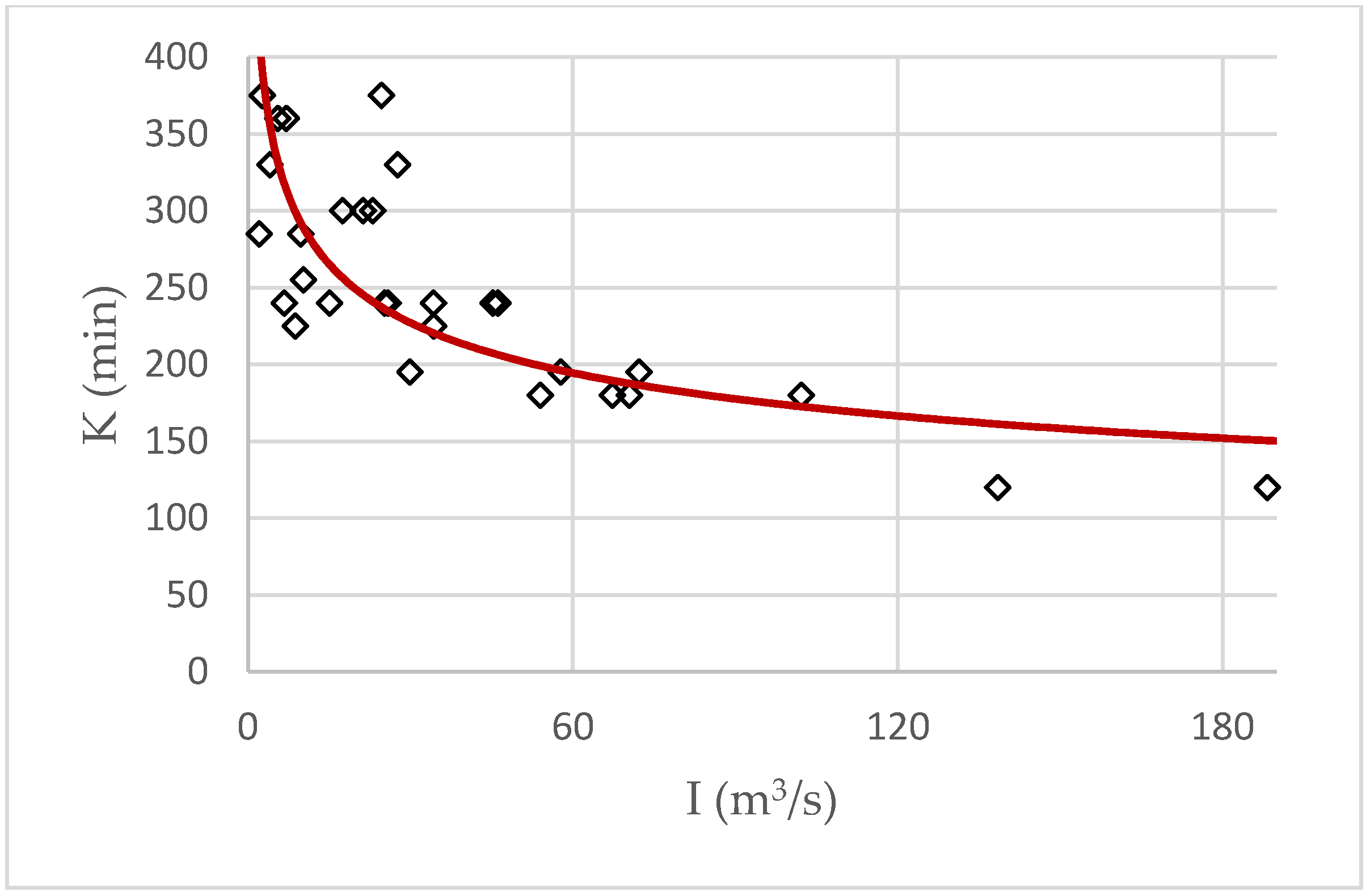
Following the lines of previous research, a variable K parameter has been used in this application [57]. In our case, K has been estimated as a function of the inflow values at the upstream station [53]. To do so, a number of peaks were previously identified in the hydrographs of the selected calibration flood events. The flood wave propagation time can be readily approximated from characteristic points on the recorded hydrographs at either end of a reach [58].
3.2. Model-2 Basic Component
This second proposed model is a simpler model than the Muskingum approach, as the outflow measured values at the end of the river reach were not involved in the basic conceptual model. They were only used in the error updating scheme. According to it, the flow forecasted value can be written in the simple form , standing for a lead time prediction of H min, being O the outflow rate (m3/s) at the downstream gauge station, and I the inflow rate (m3/s) at the upstream gauge station. σ is a non-dimensionless attenuation parameter, associated with the ratio between outflow and inflow discharge rates. Its value should be expected to be less than 1 during the rising limb of the flood hydrograph and over 1 during the hydrograph recession. Concerning H, estimates will be taken as the time lag associated with flood hydrograph routing process along the river reach. Although estimated values will be equivalent to those of Section 3.1, it is convenient to use a different notation, as the parameter itself plays a different role in this second formulation.
For a given time interval k, the conceptual model will produce an initial forecast given by the Equation (6):
where is the predicted flow value at the downstream gauge station for time (t + H). The value of will be either or , depending on the real-time situation, i.e., rising or decreasing flows, Equation (7):
Ik is the last observed flow value at Campo station, and Ik−1 is the penultimate one. A vector of n predictions is also generated, for all intermediate intervals ( min) between k and (k + H), Equation (8).
where is the forecasted value generated in the previous time step (k−1), is the one generated two-time steps before, etc.
This vector has n + 1 components, which were updated as the real-time forecasting procedure advanced. It should be noted that the length n + 1 of the vector in Equation (11) is variable, depending on the actual lead-time H.
3.3. Error Updating Scheme
A straight forward error-correction scheme was implemented, adequately coupled with each of the previously described basic conceptual models.
The forecasting error can be defined as the difference between the forecasted flow value (no matter which of the two previous basic models was used), and the really observed flow value at Graus downstream gauge station (Equation (9))
Obviously, a vector of errors is built for a given time, in each of the time steps of the real-time forecasting procedure Equation (13), in the same way as a basic model forecasts a vector of flow forecasts, i.e., Equation (8) for the case of the model-2 basic component.
The basic conceptual model forecasts values, either Muskingum or the model-2 basic component, were corrected using the previous immediate time step computed error, as indicated in Equation (11):
These estimates changed dynamically as the real-time forecasting process evolved, with the error updating term treated as a time series of pure correction of the conceptual basic model’s predictions. An upper threshold for the error correction term absolute change from one to the next time step was adopted, preventing eventual amplifications of errors that eventually originated from a given large error after the basic deterministic model estimation.
3.4. Model Evaluation
Three performance indexes have been estimated in order to assess the forecasting ability of the model to reproduce the observed discharge values at the downstream gauge station. Higher values of these indexes correspond to better performance of the model. They are described below:
r = Pearson’s correlation coefficient, Equation (12):
where Oobs (t) is the outflow discharge at Campo station and Opred (t) is the predicted discharge at Graus station. and refer to the respective average values of the series.
The NS coefficient [59], Equation (13):
where Oobs (t) is the measured flow discharge at time t in the downstream gauge station. Opred (t) is the predicted outflow value for that given time t, and is the average value of the flow discharge at the downstream gauge station. Both summations were extended over all predictions provided by the model and compared to the corresponding observed values at the Graus station.
Persistence coefficient [60,61], Equation (14):
where is the measured flow discharge at time , and is the lead time.
PC compares the forecasting error of the model to the error associated with a naïve model based on the hypothetical persistence of the flow discharge. In other words, a model for which the forecast is assumed to coincide with the most recent observed value at the downstream end of the reach. Once again, a value of the index PC = 1 would imply a perfect match of modeled discharge to the observed data, and values close to 1 indicate a good performance of the model. A value of PC = 0 would indicate that our model goodness of forecast is comparable to that of the discharge persistence naïve model, which assumes a steady-state over the forecasting lead time.
The average ratio has been also computed for both models and for each data set, where Opred is the forecasted flow value, and Oobs is the observed one. Therefore, implies flow underestimation, while indicates overestimation.
Concerning error statistics, several descriptors have been included in Section 4. First, the empirical distribution of errors is described, for calibration and validation samples. The mean and standard deviation of each of the distributions were estimated. In order to quantify the prediction uncertainty, 5% and 95% percentiles were obtained for the empirical distributions of flow forecasting errors (m3/s). Finally, the goodness of flood peak forecasts was evaluated in terms of the average errors (absolute and relative) and maximum errors, computed only over the hydrograph peaks for both samples (calibration and validation).
4. Results and Discussion
This section presents the flow forecasting results derived from the application of the two models described above. The performance indexes presented in Section 3.4 have been obtained for calibration and validation data sets, corresponding to selected historical flood hydrographs in the river Ésera (Section 2). Model-1 and model-2 results are presented in Section 4.1 and Section 4.2. A comparison of the results and discussion are presented in Section 4.3.
4.1. Results for Model-1
Firstly, Muskingum parameters were estimated for the calibration data set, for optimal representation of outflow hydrographs in terms of the time delay between inflow and outflow peaks, and peak flow values. Concerning parameter X, values estimated were in all cases close to 0.2, which is also a commonly accepted value in the literature, as stated before [52]. Thus, such a reference value was adopted herein for the present case study, providing satisfactory results. The K parameter, though, has been shown to depend strongly on discharge values (Figure 4).
For the case study analyzed herein, the estimated K values are well represented by a potential trend, Equation (15):
where and .
Model-1 was then implemented in terms of this Muskingum conceptual approach plus the error correction term described in Section 3.3. The forecasting accuracy has been tested through the indexes and error statistics introduced in Section 3.4. They have been obtained for both calibration and validation data sets (Table 2 and Table 3).
Figure 5a presents plots of the flow forecasts vs the measured flows at the downstream end of the river reach, for the calibration data set. Figure 5b shows the empirical frequency distribution of errors.
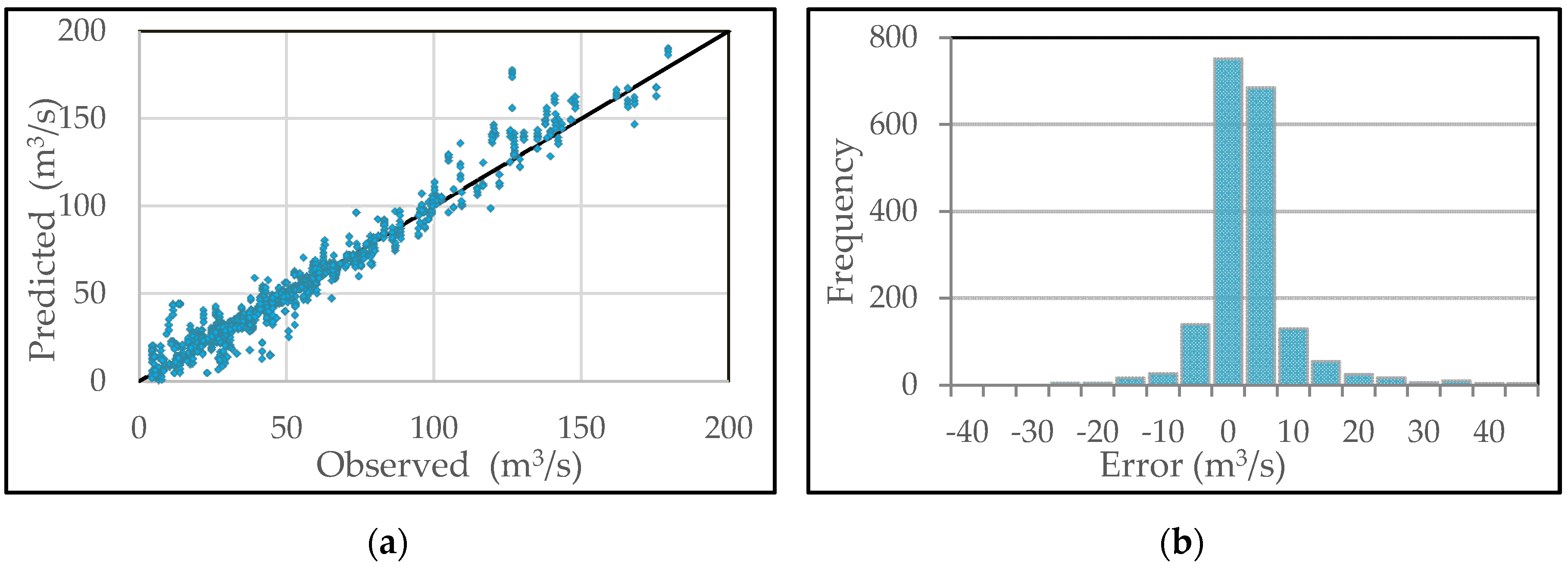
The same graphs obtained for the validation data set are shown in Figure 6a,b.
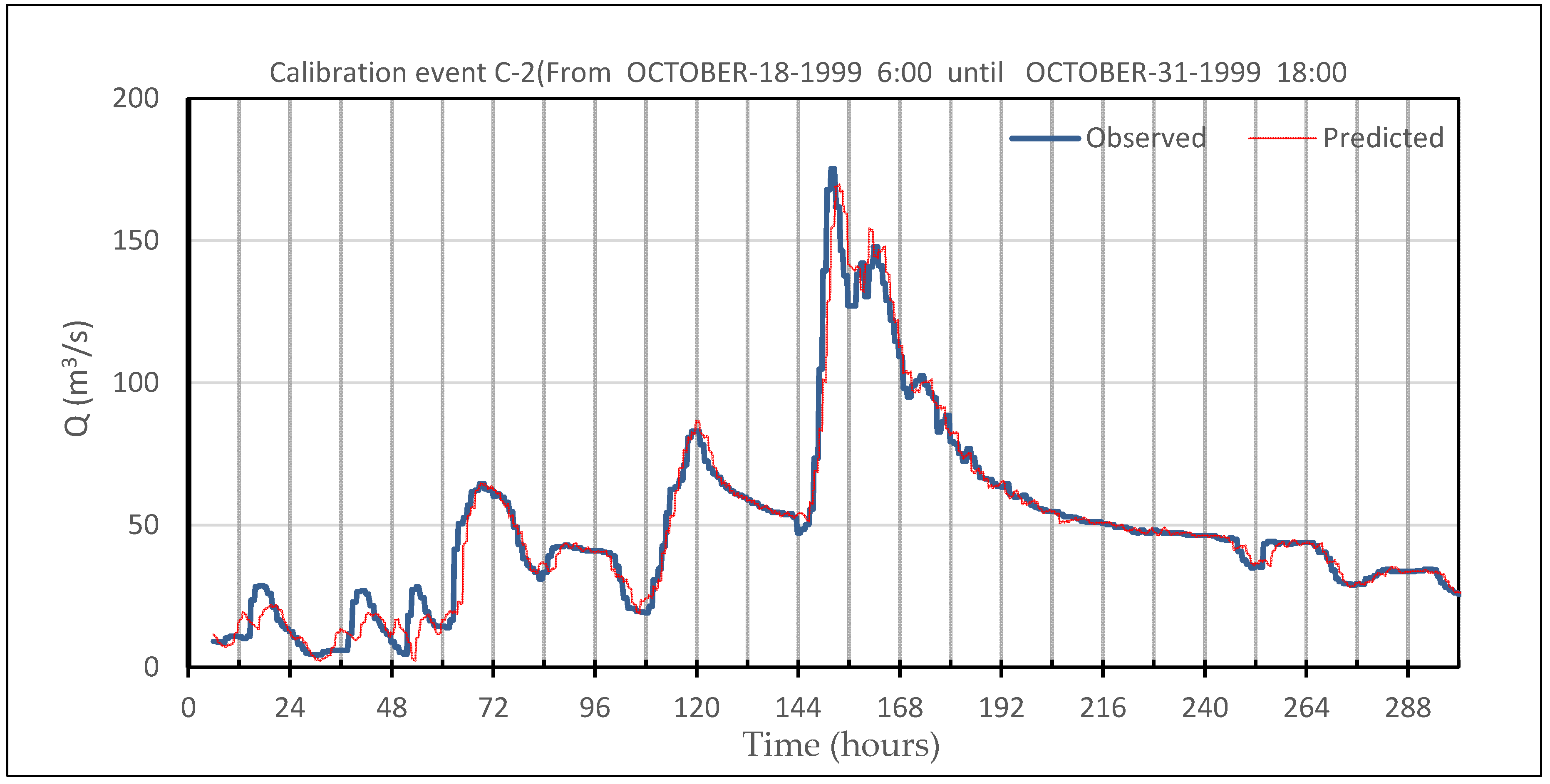
Figure 7 and Figure 8 show the flow forecasting results for two given calibration and validation flood events, respectively.
The goodness of the flood peak forecasts was evaluated in terms of the average errors (absolute and relative) computed only over several hydrograph peaks identified in both data sets. Table 4 presents the results obtained.
4.2. Results for Model-2
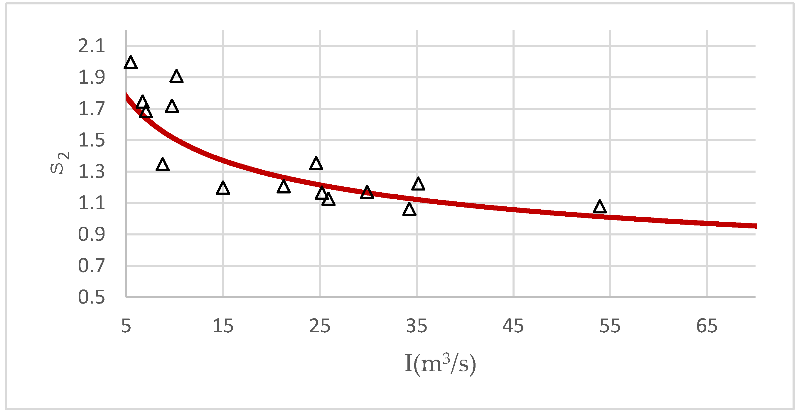
The estimation of both parameters and H introduced in Section 3.2 was carried out from the sample of calibration hydrographs. To do so, empirical data were extracted from historical hydrographs rising limbs and recession limbs, in order to estimate the average attenuation and time lags. For the rising limbs, was shown to be stable. The average value estimated was , with a standard deviation of 0.002, for the sample of calibration flow peaks. On the contrary, for the recession limbs, the value of clearly shows a decaying trend with respect to the inflow discharge I. Concerning the H values, and following previous explanation in Section 3.2, their estimates follow the empirical values in Figure 4. For clarity of formulation, we will refer now to Equation (16). Thus, for both parameters H and σ2 in model-2, the same formal functional relationship was assumed (Equations (16) and (17)):
.
Being ai and bi (i = 1,2) directly estimated from the calibration hydrograph data. For the case study considered herein, the estimated values that best represented the observed empirical relationships where (Figure 4 and Figure 9).
Figure 10a presents plots of the flow forecasts vs measured flows at the downstream end of the river reach, for the calibration data set. Figure 10b shows the empirical frequency distribution of errors.
The same graphs obtained for the validation data set are shown in Figure 11.
4.3. Comparison of Results and Discussion
The results obtained from the two models developed are discussed in this section. To do so, the computed outflow hydrograph at the Graus gauge station, at the downstream end of the river reach, was validated by comparison with the measured flow at such station. As presented in the previous section (Table 3 and Table 6), this was done for several selected lead-times, ranging from one hour to two hours. Thus, only short time real-time forecasting intervals were considered, with an upper threshold (2 h) limited by the empirically observed time lag between respective flow peaks in the calibration data set. We will refer to the validation set statistics for the discussion about the models performance.
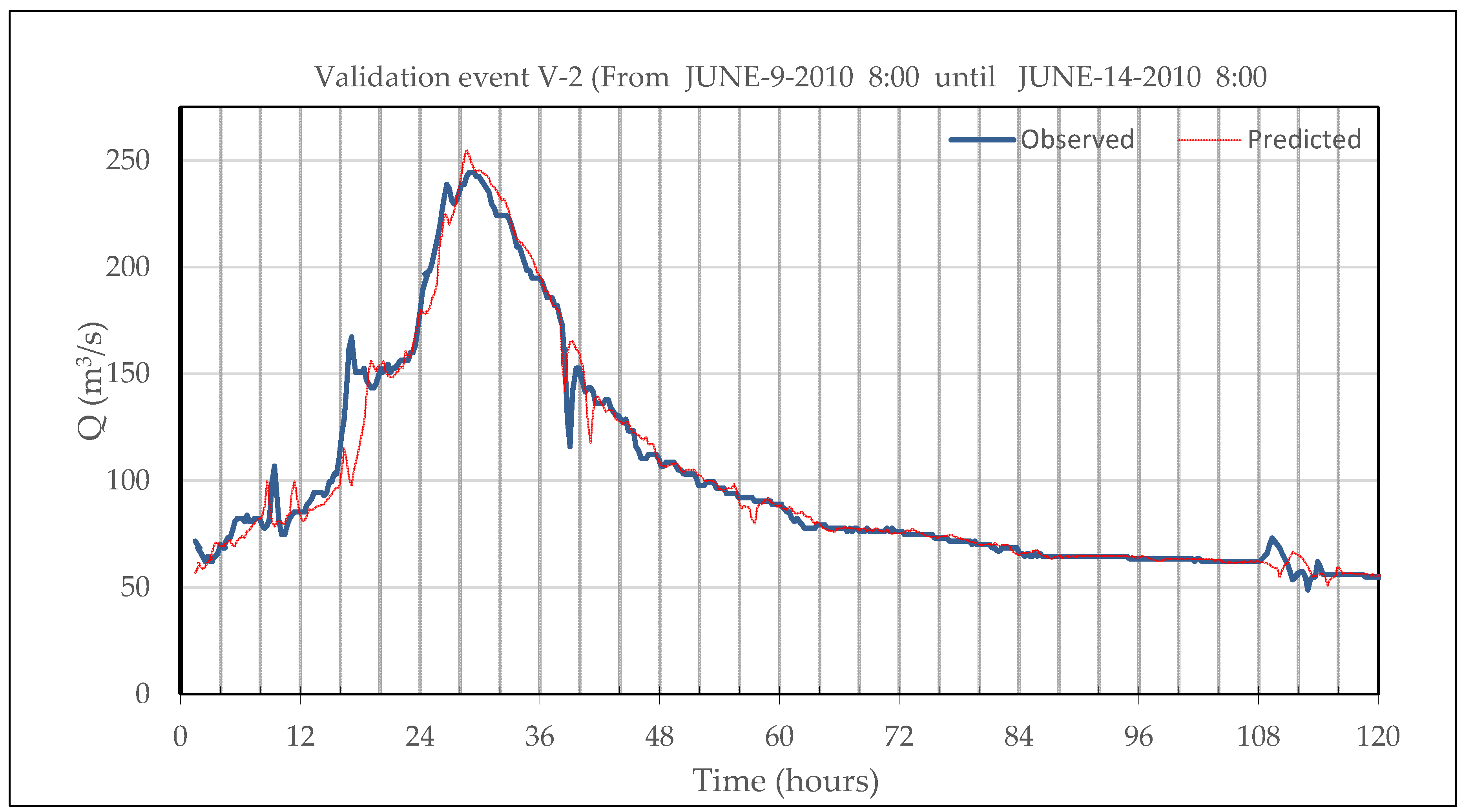
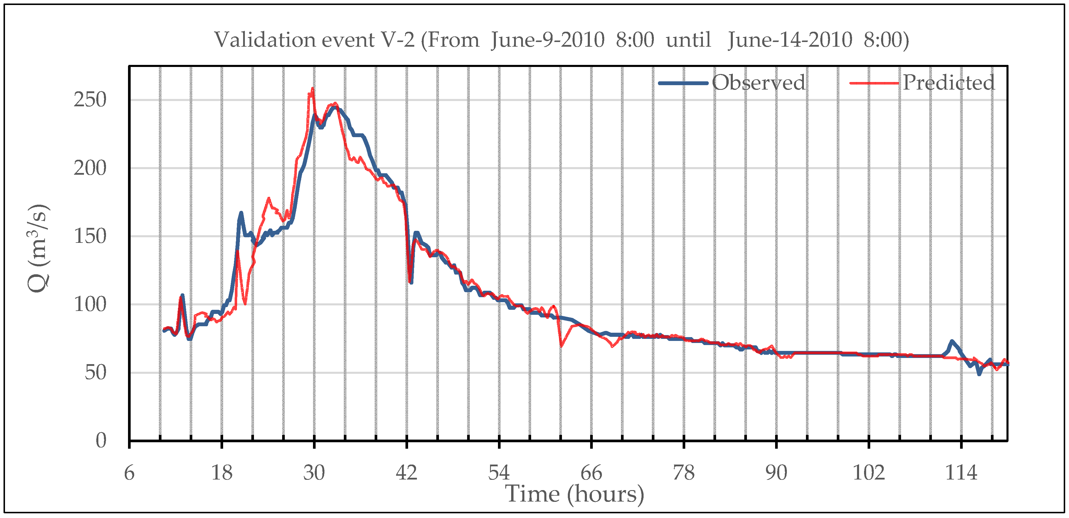
The validation results indicate a satisfactory performance of both models, with correlation coefficients of 0.985 and Nash-Sutcliffe efficiency coefficient of 0.970 when a 2 h flow forecasting lead time was considered. Figure 8 and Figure 13 show a comparison of observed vs computed values for the validation flood event V3.
For the recession limb of the hydrograph, both lines were not easily distinguishable, and thus, forecasted values showed a high level of accuracy. This was obviously not the most relevant part of the hydrograph, as operational hydrology potential benefits relied mainly on the ability of the models to accurately reproduce the rising limb, and anticipated the flood peak with maximum reliability. It was in this part of the hydrograph where some significant performance differences were found between both models tested. Model-1 reproduced better the rising limb, although none of them reproduced adequately the first observed peak (165 m3/s). The main peak of the flood event (250 m3/s), though, was correctly anticipated by both modeling schemes. With regards to the family of validation hydrographs, model-1 showed a better ability to predict more accurately the flow peaks, with flow forecasting errors under 4% (20% for model-2), for a 2 h lead-time. Model-2 tended to overestimate the hydrographs peaks (), that is, an average approximate overestimation of around 6%.
The general performance of model-1 was slightly better. The forecasting error standard deviation was approximately 7 m3/s, versus 9 m3/s for model-2. On the other hand, model-2 tended to overestimate outflows (average values over 1, for all the lead-times considered in the case study), while values remained very close to 1 for the model-1 flow real-time forecasts.
Another interesting behavior of the tested models concerns the variation of the performance indexes when the forecasting lead-time was increased. The results presented in Table 2, Table 3, Table 5 and Table 6 clearly indicate that there was no significant deterioration of the accuracy when the lead time changed from 1 h to 2 h. This result is consistent with the fact that basic conceptual formulations represented by Equations (5) and (8), respectively, that were only applied for lead-times matching estimated flood wave propagation times along the river reach [62,63]. These have been shown to vary during the flood event but remained well over 1 h for the presented case study. Thus, intermediate forecasted values for smaller lead-times resulted basically from the real-time error-correction scheme implemented, described in Section 3.2. Concerning forecasting confidence intervals, Table 2, Table 3, Table 5 and Table 6 show that for shorter lead-times there was less uncertainty, although the forecasting accuracy does not vary significantly as the lead-time was extended to two hours.
On the contrary, PC values clearly increased as the lead-time was extended, proving the relative merit of the models to enhance future flows knowledge, as compared to the flow persistence naïve hypothesis. In fact, PC coefficient estimates were over 0.6 for a 2 h lead time, falling down to smaller values (0.2) for a 1 h lead-time. For very short lead-times (under 30 min), the relative contribution of the developed models should be considered almost negligible when compared to the trivial flow persistence hypothesis.
It should be remarked that the conceptual component of model-1 was based on the classic Muskingum formulation, conveniently adapted to real-time requirements. As such, real-time measurements of both ends of the river were actually used in Equation (5). On the contrary, the model-2 basic component only involved upstream real-time measurements (Equation (8)). From this point of view, model-1 should be expected to present better performance than model-2, as it actually did. However, as discussed above, differences between them were not very significant. This fact proves the prevailing role of the error-correction scheme when short-term forecasts were generated, as it the case of the presented case study. This remark is also consistent with the fact that no explicit account of possible lateral inflows (or eventual losses along the river reach) has been introduced in the basic conceptual formulations, nor in Equation (5) or Equation (8).
While the quality of the forecasting results is comparable to previous research on short-term flow forecasting, two interesting aspects should be outlined concerning the results obtained herein. The first one is related to the fact that very short lead times yield efficient and accurate predictions but at the same time, the PC index deteriorated to the point where no actual improvement from a flow persistence naïve model was obtained. The second one is related to the evaluation of the relative merit and actual role played by the conceptual part of the models. While the model-2 basic component was not comparable on a theoretical basis to the well-established Muskingum scheme, the quality of the results was quite similar. This puts into the spotlight the practical relevance of the error updating scheme in the real-time operational context.
5. Conclusions
The research presented herein analyzed the behavior of simple real-time forecasting techniques implemented in a small mountain catchment located in the Pyrenees, North of Spain. The hydrological response, in this case, was particularly fast, due to the steep slopes and the resulting high average flow velocities during floods events, which can be considered typical flash-flood events. Two gauge stations, Campo and Graus, are respectively located at the upstream and downstream end of the analyzed river reach. For high flow values, the flood hydrograph movement along the reach took approximately 2 h.
Several small hydraulic power plants (<100 MW power) are located upstream Campo gauge station, as previously explained in Section 2.1, introducing some fluctuations in the river flow due to turbine operations. There is no available information concerning detailed turbine operations in the power plants, but they are obviously reflected directly in the measured discharges at the Campo gauge station, which is located only 0.3 km downstream of the Campo power plant. The observed flow fluctuations in this gauge station were attenuated along the 36 km length reach, as water flows downstream. However, they can affect downstream infrastructure in different ways. The models tested herein can estimate the time required to reach the downstream end, and also the expected flow attenuation, in order to assess potential downstream affections. It is precisely this anticipation that can provide the basis for optimal decisions in real-time. On the other hand, the ability of the models to reproduce the routing process along the river reach makes them useful to assess required limitations concerning turbine operation to ensure downstream flow conditions within advisable fluctuations.
In these terms, the pursued objective in this research was the generation of reliable real-time flow forecasts at the Graus station, for lead times between 1 and 2 h. Highly parsimonious hydrological routines have been implemented, enhanced with a simple real-time error updating scheme. Their characteristics were suited to the requirements of typical tools for real-time short term flow forecasts. Thus, they were simple, robust and easily programmed, allowing a straight-forward practical implementation in a given operational hydrology context.
The results obtained show that both tested models were adequate as they reproduced with good accuracy the peak flows observed in the downstream gauge station for lead times up to the flood wave propagation time. The first model, based on the Muskingum classical formulation, slightly over-performed the second one, which was derived from an even simpler formulation. Both methods proved to be computationally efficient and fully adapted to the requirements of operational hydrology for real time management.
The PC performance coefficient was estimated, in order to quantify the relative merits of the models to enhance knowledge of future flows, as compared to the flow persistence naïve hypothesis. The resultant PC coefficients were over 0.6 for the 2 h lead time. Summing up, Muskingum’s basic formulation with an added simple error updating scheme provided a useful practical response to the engineering problem outlined above. However, the importance of the latter term is outlined, as previously explained in Section 4.3.
This applied even if no particular assumption concerning lateral inflows along the river reach was made. In other words, the method can be applied with or without the significant presence of effective rainfall, as the real-time error correction algorithm implicitly accounted for the potential lateral inflows due to rainfall-runoff processes taking place in the catchment. Although these are not relevant in the particular case-study considered herein, further research will be conducted for other cases.
Author Contributions
Conceptualization, N.M., J.Á.A. and R.G.-B.; Data curation, N.M. and J.Á.A.; Formal analysis, J.Á.A. and R.G.-B.; Investigation, N.M. and J.Á.A.; Methodology, N.M. and R.G.-B.; Project administration, R.G.-B.; Resources, J.Á.A.; Software, N.M.; Supervision, R.G.-B.; J.Á.A. and R.G.-B.; Visualization, J.Á.A.; Writing—original draft, N.M., J.Á.A. and R.G.-B.; Writing—review and editing, R.G.-B. All authors have read and agreed to the published version of the manuscript.
Funding
This research received no external funding.
Acknowledgments
The authors wish to acknowledge support from Confederación Hidrográfica del Ebro.
Conflicts of Interest
The authors declare no conflict of interest.
References
- Moramarco, T.; Barbetta, S.; Melone, F.; Singh, V.P. A real-time stage Muskingum forecasting model for a site without rating curve. Hydrol. Sci. J. 2006, 51, 66–82. [Google Scholar] [CrossRef]
- Perumal, M.; Moramarco, T.; Barbetta, S.; Melone, F.; Sahoo, B. Real-time flood stage forecasting by Variable Parameter Muskingum Stage hydrograph routing method. Hydrol. Res. 2011, 42, 150–161. [Google Scholar] [CrossRef]
- McCarthy, G. The unit hydrograph and flood routing. In Proceedings of the Conference North Atlantic Divsion, Chapel Hill, NC, USA, 20–25 April 1938. [Google Scholar]
- Clark, C.O. Storage and the Unit Hydrograph. Trans. Am. Soc. Civ. Eng. 1945, 110, 1419–1446. [Google Scholar]
- Te Chow, V. Open-Channel Hydraulics; McGraw-Hill Book Company: New York, NY, USA, 1959; pp. 507–510. [Google Scholar]
- Nash, J.E. The Form of the Instantaneous Unit Hydrograph; International Association of Scientific Hydrology: Wallingford, UK, 1957. [Google Scholar]
- Cunge, J.A. On The Subject Of A Flood Propagation Computation Method (Musklngum Method). J. Hydraul. Res. 1969, 7, 205–230. [Google Scholar] [CrossRef]
- Dooge, J.C.; Strupczewski, W.G.; Napiorkowski, J. Hydrodynamic derivation of storage parameters of the Muskingum model. J. Hydrol. 1982, 54, 371–387. [Google Scholar] [CrossRef]
- Ponce, V.M.; Yevjevich, V. Muskingum-Cunge method with variable parameters. J. Hydraul. Div. 1978, 104, 1663–1667. [Google Scholar] [CrossRef]
- Ponce, V.M.; Theurer, F.D. Accuracy Criteria in Diffusion Routing. J. Hydraul. Eng. 1983, 109, 806–807. [Google Scholar] [CrossRef]
- Kundzewicz, Z.W. Physically based hydrological flood routing methods. Hydrol. Sci. J. 1986, 31, 237–261. [Google Scholar] [CrossRef] [Green Version]
- Singh, V.P. Kinematic Wave Modeling in Water Resources. Surface-Water Hydrology; John Wiley: Chichester, UK, 1996. [Google Scholar]
- Singh, V.P.; Scarlatos, P.D. Analysis of Nonlinear Muskingum Flood Routing. J. Hydraul. Eng. 1987, 113, 61–79. [Google Scholar] [CrossRef]
- Perumal, M. Multilinear Muskingum flood routing method. J. Hydrol. 1992, 133, 259–272. [Google Scholar] [CrossRef]
- Perumal, M. Removing some anomalies of the Muskingum method. Watershed Hydrol. 2003, 6, 180. [Google Scholar]
- Ponce, V.; Changanti, P. Variable-parameter Muskingum-Cunge method revisited. J. Hydrol. 1994, 162, 433–439. [Google Scholar] [CrossRef]
- Tang, X.; Knight, D.W.; Samuels, P. Variable parameter Muskingum-Cunge method for flood routing in a compound channel. J. Hydraul. Res. 1999, 37, 591–614. [Google Scholar] [CrossRef]
- Al-Humoud, J.M.; Esen, I.I. Approximate Methods for the Estimation of Muskingum Flood Routing Parameters. Water Resour. Manag. 2006, 20, 979–990. [Google Scholar] [CrossRef]
- Todini, E. A mass conservative and water storage consistent variable parameter Muskingum-Cunge approach. Hydrol. Earth Syst. Sci. 2007, 11, 1645–1659. [Google Scholar] [CrossRef] [Green Version]
- Brakensiek, D.L. Estimating coefficients for storage flood routing. J. Geophys. Res. Space Phys. 1963, 68, 6471–6474. [Google Scholar] [CrossRef]
- Birkhead, A.; James, C. Muskingum river routing with dynamic bank storage. J. Hydrol. 2002, 264, 113–132. [Google Scholar] [CrossRef]
- Xiaofang, R.; Fanggui, L.; Mei, Y. Discussion of Muskingum method parameter X. Water Sci. Eng. 2008, 1, 16–23. [Google Scholar]
- Perumal, M.; Price, R.K. A fully mass conservative variable parameter McCarthy–Muskingum method: Theory and verification. J. Hydrol. 2013, 502, 89–102. [Google Scholar] [CrossRef]
- O’Donnell, T. A direct three-parameter Muskingum procedure incorporating lateral inflow. Hydrol. Sci. J. 1985, 30, 479–496. [Google Scholar] [CrossRef] [Green Version]
- Kshirsagar, M.; Rajagopalan, B.; Lal, U. Optimal parameter estimation for Muskingum routing with ungauged lateral inflow. J. Hydrol. 1995, 169, 25–35. [Google Scholar] [CrossRef]
- Barbetta, S.; Brocca, L.; Melone, F.; Moramarco, T. On the lateral inflows assessment within a real-time stage monitoring addressed to flood forecasting. In Proceedings of the 4th International Congress on Environmental Modelling and Software, iEMSs 2008, Barcelona, Spain, 7–10 July 2008; Volume 1, pp. 438–445. [Google Scholar]
- Yadav, B.; Perumal, M.; Bárdossy, A. Variable parameter McCarthy–Muskingum routing method considering lateral flow. J. Hydrol. 2015, 523, 489–499. [Google Scholar] [CrossRef]
- Perumal, M. Hydrodynamic derivation of a variable parameter Muskingum method: 1. Theory and solution procedure. Hydrol. Sci. J. 1994, 39, 431–442. [Google Scholar] [CrossRef] [Green Version]
- Perumal, M.; O’Connell, E.; Raju, K.G.R. Field Applications of a Variable-Parameter Muskingum Method. J. Hydrol. Eng. 2001, 6, 196–207. [Google Scholar] [CrossRef]
- Perumal, M.; Sahoo, B. Applicability criteria of the variable parameter Muskingum stage and discharge routing methods. Water Resour. Res. 2007, 43. [Google Scholar] [CrossRef]
- Gill, M.A. Flood routing by the Muskingum method. J. Hydrol. 1978, 36, 353–363. [Google Scholar] [CrossRef]
- Tung, Y. River Flood Routing by Nonlinear Muskingum Method. J. Hydraul. Eng. 1985, 111, 1447–1460. [Google Scholar] [CrossRef] [Green Version]
- Papamichail, D.M.; Georgiou, P.E. River flood routing by a nonlinear form of the Muskingum method. In Proceedings of the 5th Conference of the Greek Hydrotechnical Association, Larisa, Greece, 3–6 July 1992; pp. 141–149. [Google Scholar]
- Yoon, J.; Padmanabhan, G. Parameter estimation of linear and nonlinear Muskingum models. J. Water Resour. Plan. Manag. 1993, 119, 600–610. [Google Scholar] [CrossRef]
- Mohan, S. Parameter Estimation of Nonlinear Muskingum Models Using Genetic Algorithm. J. Hydraul. Eng. 1997, 123, 137–142. [Google Scholar] [CrossRef]
- Luo, J.; Xie, J. Parameter Estimation for Nonlinear Muskingum Model Based on Immune Clonal Selection Algorithm. J. Hydrol. Eng. 2010, 15, 844–851. [Google Scholar] [CrossRef]
- Kang, L.; Zhang, S. Application of the Elitist-Mutated PSO and an Improved GSA to Estimate Parameters of Linear and Nonlinear Muskingum Flood Routing Models. PLoS ONE 2016, 11, e0147338. [Google Scholar] [CrossRef] [PubMed]
- Geem, Z.W. Parameter Estimation for the Nonlinear Muskingum Model Using the BFGS Technique. J. Irrig. Drain. Eng. 2006, 132, 474–478. [Google Scholar] [CrossRef]
- Chu, H.-J.; Chang, L.-C. Applying Particle Swarm Optimization to Parameter Estimation of the Nonlinear Muskingum Model. J. Hydrol. Eng. 2009, 14, 1024–1027. [Google Scholar] [CrossRef]
- Barati, R. Parameter Estimation of Nonlinear Muskingum Models Using Nelder-Mead Simplex Algorithm. J. Hydrol. Eng. 2011, 16, 946–954. [Google Scholar] [CrossRef]
- Karahan, H.; Gurarslan, G.; Geem, Z.W. Parameter Estimation of the Nonlinear Muskingum Flood-Routing Model Using a Hybrid Harmony Search Algorithm. J. Hydrol. Eng. 2013, 18, 352–360. [Google Scholar] [CrossRef]
- Chen, X.; Chau, K.-W.; Busari, A. A comparative study of population-based optimization algorithms for downstream river flow forecasting by a hybrid neural network model. Eng. Appl. Artif. Intell. 2015, 46, 258–268. [Google Scholar] [CrossRef]
- Latt, Z.Z. Application of Feedforward Artificial Neural Network in Muskingum Flood Routing: A Black-Box Forecasting Approach for a Natural River System. Water Resour. Manag. 2015, 29, 4995–5014. [Google Scholar] [CrossRef]
- Niazkar, M.; Afzali, S.H. Application of New Hybrid Optimization Technique for Parameter Estimation of New Improved Version of Muskingum Model. Water Resour. Manag. 2016, 30, 4713–4730. [Google Scholar] [CrossRef]
- Dong, S.; Su, B.; Zhang, Y. Optimization Estimation of Muskingum Model Parameter Based on Genetic Algorithm. In Recent Advances in Computer Science and Information Engineering; Springer: Berlin/Heidelberg, Germany, 2012; pp. 563–569. [Google Scholar]
- Kucukkoc, I.; Zhang, D.Z. Integrating ant colony and genetic algorithms in the balancing and scheduling of complex assembly lines. Int. J. Adv. Manuf. Technol. 2015, 82, 265–285. [Google Scholar] [CrossRef] [Green Version]
- Bazargan, J.; Norouzi, H. Investigation the Effect of Using Variable Values for the Parameters of the Linear Muskingum Method Using the Particle Swarm Algorithm (PSO). Water Resour. Manag. 2018, 32, 4763–4777. [Google Scholar] [CrossRef]
- Ehteram, M.; Mousavi, S.F.; Karami, H.; Farzin, S.; Singh, V.P.; Chau, K.-W.; El-Shafie, A. Reservoir operation based on evolutionary algorithms and multi-criteria decision-making under climate change and uncertainty. J. Hydroinform. 2018, 20, 332–355. [Google Scholar] [CrossRef]
- Pei, J.; Su, Y.; Zhang, D. Fuzzy energy management strategy for parallel HEV based on pigeon-inspired optimization algorithm. Sci. China Ser. E Technol. Sci. 2016, 60, 425–433. [Google Scholar] [CrossRef]
- Schumm, S.A. Evolution of drainage systems and slopes in badlands at perth amboy, New Jersey. GSA Bull. 1956, 67, 597. [Google Scholar] [CrossRef]
- Fread, D.L. Flow Routing in Handbook of Hydrology; Maidment, D.R., Ed.; McGraw-Hill Inc.: New York, NY, USA, 1993. [Google Scholar]
- McCuen, R.H. Hydrologic Analysis and Design; Prentice-Hall: Englewood Cliffs, NJ, USA, 1989. [Google Scholar]
- Balaz, M.; Danáčová, M.; Szolgay, J. On the use of the Muskingum method for the simulation of flood wave movements. Slovak J. Civ. Eng. 2010, 18, 14–20. [Google Scholar] [CrossRef] [Green Version]
- Franchini, M.; Lamberti, P. A flood routing Muskingum type simulation and forecasting model based on level data alone. Water Resour. Res. 1994, 30, 2183–2196. [Google Scholar] [CrossRef]
- Yadav, P.; Singh, N.; Goel, P.S.; Itabashi-Campbell, R. A framework for reliability prediction during product development process incorporating engineering judgments. Qual. Eng. 2003, 15, 649–662. [Google Scholar] [CrossRef]
- Tayfur, G. Soft Computing in Water Resources Engineering: Artificial Neural Networks, Fuzzy Logic and Genetic Algorithms; WIT Press: Southampton, NY, USA, 2014. [Google Scholar]
- Song, X.-M.; Kong, F.-Z.; Zhu, Z.-X. Application of Muskingum routing method with variable parameters in ungauged basin. Water Sci. Eng 2011, 4, 1–12. [Google Scholar]
- Weinmann, P.E.; Laurenson, E.M. Approximate flood routing methods: A review. J. Hydraul. Div. 1979, 105, 1521–1536. [Google Scholar]
- Nash, J.E.; Sutcliffe, J.V. River flow forecasting through conceptual models part I—A discussion of principles. J. Hydrol. 1970, 10, 282–290. [Google Scholar] [CrossRef]
- Kitanidis, P.K.; Bras, R.L. Real-time forecasting with a conceptual hydrologic model: 2. Applications and results. Water Resour. Res. 1980, 16, 1034–1044. [Google Scholar] [CrossRef]
- Franchini, M.; Bernini, A.; Barbetta, S.; Moramarco, T. Forecasting discharges at the downstream end of a river reach through two simple Muskingum based procedures. J. Hydrol. 2011, 399, 335–352. [Google Scholar] [CrossRef]
- Alhumoud, J.M.; Almashan, N. Muskingum Method with Variable Parameter Estimation. Math. Model. Eng. Probl. 2019, 6, 355–362. [Google Scholar] [CrossRef]
- Yang, R.; Hou, B.; Xiao, W.; Liang, C.; Zhang, X.; Li, B.; Yu, H. The applicability of real-time flood forecasting correction techniques coupled with the Muskingum method. Hydrol. Res. 2019, 51, 17–29. [Google Scholar] [CrossRef] [Green Version]
Figure 1.
Ésera River catchment.

Figure 2.
Hydroelectric power plants location.

Figure 3.
Observed hydrograph at Campo and Graus gauge stations (event C3).

Figure 4.
Empirical estimation of K as a function of inflow values at the Campo gauge station.

Figure 5.
(a) Flow forecasts vs measured flows at the Graus station. (b) Empirical frequency distribution of the errors (calibration data set).
Figure 5.
(a) Flow forecasts vs measured flows at the Graus station. (b) Empirical frequency distribution of the errors (calibration data set).

Figure 6.
(a) Flow forecasts vs measured flows at the Graus station. (b) Empirical frequency distribution of the errors (validation data set).
Figure 6.
(a) Flow forecasts vs measured flows at the Graus station. (b) Empirical frequency distribution of the errors (validation data set).

Figure 7.
Comparison of flow forecasts and observed outflows at the Graus station (calibration event C-2).
Figure 7.
Comparison of flow forecasts and observed outflows at the Graus station (calibration event C-2).

Figure 8.
Comparison of 2 h lead time flow forecasts and observed outflows at the Graus station (validation event V3).
Figure 8.
Comparison of 2 h lead time flow forecasts and observed outflows at the Graus station (validation event V3).

Figure 9.
Empirical estimation of attenuation parameter—recession limb of the hydrograph.

Figure 10.
(a) Flow forecasts vs measured flows at the Graus station (left). (b) Empirical frequency distribution of the errors (calibration data set) (right).
Figure 10.
(a) Flow forecasts vs measured flows at the Graus station (left). (b) Empirical frequency distribution of the errors (calibration data set) (right).

Figure 11.
(a) Flow forecasts vs measured flows at the Graus station. (b) Empirical frequency distribution of the errors (validation data set).
Figure 11.
(a) Flow forecasts vs measured flows at the Graus station. (b) Empirical frequency distribution of the errors (validation data set).

Figure 12.
Comparison of flow forecasts and observed outflows at the Graus station (calibration event C2).
Figure 12.
Comparison of flow forecasts and observed outflows at the Graus station (calibration event C2).

Figure 13.
Comparison of 2 h lead time flow forecasts and observed outflows at the Graus station (validation event V3).
Figure 13.
Comparison of 2 h lead time flow forecasts and observed outflows at the Graus station (validation event V3).


Table 1.
Historical floods statistics.
| Event | Initial Date | Qmax Campo (m3/s) | Qmax Graus (m3/s) | Volume Campo (106 m3) | Volume Graus (106 m3) | Time lag (hour) |
|---|---|---|---|---|---|---|
| Calibration Events | ||||||
| C1 | 19 September 1999 | 154.8 | 127.8 | 18.2 | 17.7 | 1.75 |
| C2 | 18 October 1999 | 169.4 | 145.0 | 49.1 | 46.8 | 2.00 |
| C3 | 22 November 2000 | 103.7 | 95.7 | 11.0 | 11.1 | 2.50 |
| C4 | 20 October 2004 | 64.8 | 56.8 | 7.7 | 7.0 | 3.25 |
| Validation Events | ||||||
| V1 | 22 September 2006 | 117.5 | 109.7 | 21.1 | 22.8 | 2.25 |
| V2 | 16 October 2006 | 210.5 | 178.7 | 65.4 | 56.6 | 3.25 |
| V3 | 08 June 2010 | 229.1 | 219.8 | 34.7 | 39.4 | 2.75 |
| V4 | 1 November 2011 | 151.7 | 158.1 | 19.8 | 28.3 | 2.50 |
Table 2.
Model-1 performance evaluation coefficients and forecasting error statistics (calibration data set).
Table 2.
Model-1 performance evaluation coefficients and forecasting error statistics (calibration data set).
| Lead Time (min) | Calibration | Error Distribution | 5% and 95% Percentiles | |||||
|---|---|---|---|---|---|---|---|---|
| r | NS | PC | Mean (m3/s) | Std. dev. (m3/s) | Err. (m3/s) | |||
| 60 | 0.986 | 0.971 | 0.244 | 1.026 | −0.038 | 5.077 | −7.28 | 7.75 |
| 75 | 0.984 | 0.968 | 0.401 | 1.030 | −0.029 | 5.268 | −7.93 | 7.96 |
| 90 | 0.982 | 0.963 | 0.489 | 1.034 | −0.015 | 5.331 | −7.88 | 8.24 |
| 105 | 0.980 | 0.959 | 0.536 | 1.038 | −0.037 | 5.342 | −8.01 | 8.00 |
| 120 | 0.978 | 0.954 | 0.574 | 1.045 | −0.060 | 5.360 | −8.01 | 7.97 |
Table 3.
Model-1 performance evaluation coefficients and forecasting error statistics (validation data set).
Table 3.
Model-1 performance evaluation coefficients and forecasting error statistics (validation data set).
| Lead Time (min) | VALIDATION | Error Distribution | 5% and 95% Percentiles | |||||
|---|---|---|---|---|---|---|---|---|
| r | NS | PC | Mean (m3/s) | Std. dev. (m3/s) | Err. (m3/s) | |||
| 60 | 0.987 | 0.974 | 0.205 | 0.996 | −0.110 | 6.777 | −10.29 | 9.29 |
| 75 | 0.987 | 0.974 | 0.387 | 0.997 | −0.104 | 6.911 | −10.40 | 9.45 |
| 90 | 0.986 | 0.973 | 0.491 | 0.998 | −0.108 | 6.963 | −10.46 | 9.41 |
| 105 | 0.986 | 0.972 | 0.557 | 0.999 | −0.110 | 6.986 | −10.58 | 9.37 |
| 120 | 0.985 | 0.970 | 0.601 | 1.001 | −0.121 | 6.996 | −10.59 | 9.37 |
Table 4.
Error statistics estimated over a selected family of peak flows in both samples.
| Average | Maximum | |||||||
|---|---|---|---|---|---|---|---|---|
| Lead Time (min) | h | Absolute Error m3/s | Relative. Error% | Min h sub | Max h over | Absolute Error m3/s | Relative. Error % | |
| Calibration | 120 | 0.972 | −3.581 | −2.822 | 0.955 | 0.986 | −6.77 | −4.54 |
| Validation | 120 | 1.059 | 9.712 | 5.945 | 0.997 | 1.193 | 31.38 | 19.33 |
Table 5.
Model-2 performance evaluation coefficients and forecasting error statistics (calibration data set).
Table 5.
Model-2 performance evaluation coefficients and forecasting error statistics (calibration data set).
| Lead Time (min) | Calibration | Error Distribution | 5% and 95% Percentiles | |||||
|---|---|---|---|---|---|---|---|---|
| r | NS | PC | Mean(m3/s) | Std. dev(m3/s) | Err.(m3/s) | |||
| 60 | 0.984 | 0.965 | 0.468 | 0.818 | −0.728 | 6.186 | −10.80 | 5.99 |
| 75 | 0.983 | 0.963 | 0.570 | 1.008 | −0.751 | 6.487 | −11.45 | 6.90 |
| 90 | 0.982 | 0.960 | 0.631 | 1.014 | −0.745 | 6.790 | −11.44 | 7.09 |
| 105 | 0.981 | 0.958 | 0.676 | 1.024 | −0.727 | 7.129 | −11.56 | 7.36 |
| 120 | 0.979 | 0.955 | 0.712 | 0.890 | −0.723 | 7.460 | −12.07 | 7.66 |
Table 6.
Model-2 performance evaluation coefficients and forecasting error statistics (validation data set).
Table 6.
Model-2 performance evaluation coefficients and forecasting error statistics (validation data set).
| Lead Time (min) | Validation | Error Distribution | 5% and 95% Percentiles | |||||
|---|---|---|---|---|---|---|---|---|
| r | NS | PC | mean(m3/s) | Std. dev(m3/s) | Err.(m3/s) | |||
| 60 | 0.988 | 0.977 | 0.318 | 1.006 | −0.560 | 8.486 | −10.25 | 9.09 |
| 75 | 0.988 | 0.975 | 0.465 | 1.006 | −0.549 | 8.695 | −9.84 | 9.47 |
| 90 | 0.987 | 0.974 | 0.545 | 1.006 | −0.567 | 8.869 | −11.01 | 9.98 |
| 105 | 0.986 | 0.972 | 0.601 | 1.007 | −0.546 | 8.997 | −11.42 | 10.63 |
| 120 | 0.985 | 0.970 | 0.648 | 1.008 | −0.483 | 9.096 | −12.79 | 11.19 |
Table 7.
Error statistics estimated over a selected family of peak flows in both samples.
| Average | Maximum | |||||||
|---|---|---|---|---|---|---|---|---|
| Lead Time (min) | h | Absolute Error m3/s | Relative Error % | Min h sub | Max h over | Absolute Error m3/s | Relative. Error % | |
| Calibration | 120 | 1.031 | 3.630 | 3.060 | 0.958 | 1.114 | 12.68 | 11.44 |
| Validation | 120 | 1.059 | 9.712 | 5.945 | 0.997 | 1.193 | 31.38 | 19.33 |
© 2020 by the authors. Licensee MDPI, Basel, Switzerland. This article is an open access article distributed under the terms and conditions of the Creative Commons Attribution (CC BY) license (http://creativecommons.org/licenses/by/4.0/).
Share and Cite
MDPI and ACS Style
Montes, N.; Aranda, J.Á.; García-Bartual, R. Real Time Flow Forecasting in a Mountain River Catchment Using Conceptual Models with Simple Error Correction Scheme. Water 2020, 12, 1484. https://doi.org/10.3390/w12051484
AMA Style
Montes N, Aranda JÁ, García-Bartual R. Real Time Flow Forecasting in a Mountain River Catchment Using Conceptual Models with Simple Error Correction Scheme. Water. 2020; 12(5):1484. https://doi.org/10.3390/w12051484
Chicago/Turabian StyleMontes, Nicolás, José Ángel Aranda, and Rafael García-Bartual. 2020. "Real Time Flow Forecasting in a Mountain River Catchment Using Conceptual Models with Simple Error Correction Scheme" Water 12, no. 5: 1484. https://doi.org/10.3390/w12051484
Note that from the first issue of 2016, this journal uses article numbers instead of page numbers. See further details here.