Accelerating Contaminant Transport Simulation in MT3DMS Using JASMIN-Based Parallel Computing


1
School of Water Resources and Environment, China University of Geosciences (Beijing), Beijing 100083, China
2
China Nuclear Power Engineering Co. Ltd., Beijing 100840, China
3
Institute of Applied Physics and Computational Mathematics, Beijing 100088, China
4
CAEP Software Center for High Performance Numerical Simulation, Beijing 100088, China
*
Author to whom correspondence should be addressed.
Water 2020, 12(5), 1480; https://doi.org/10.3390/w12051480
Submission received: 9 April 2020
/
Revised: 19 May 2020
/
Accepted: 19 May 2020
/
Published: 22 May 2020
(This article belongs to the Special Issue Groundwater and Soil Remediation)
Abstract
:To overcome the large time and memory consumption problems in large-scale high-resolution contaminant transport simulations, an efficient approach was presented to parallelize the modular three-dimensional transport model for multi-species (MT3DMS) (University of Alabama, Tuscaloosa, AL, USA) program on J adaptive structured meshes applications infrastructures (JASMIN). In this approach, a domain decomposition method and a stencil-based method were used to accomplish parallel implementation, while a ghost cell strategy was used for communication. The MODFLOW-MT3DMS coupling mode was optimized to achieve the parallel coupling of flow and contaminant transport. Five types of models were used to verify the correctness and test the parallel performance of the method. The developed parallel program JMT3D (China University of Geosciences (Beijing), Beijing, China) can increase the speed by up to 31.7 times, save memory consumption by 96% with 46 processors, and ensure that the solution accuracy and convergence do not decrease as the number of domains increases. The BiCGSTAB (Bi-conjugate gradient variant algorithm) method required the least amount of time and achieved high speedup in most cases. Coupling the flow and contaminant transport further improved the efficiency of the simulations, with a 33.45 times higher speedup achieved on 46 processors. The AMG (algebraic multigrid) method achieved a good scalability, with an efficiency above 100% on hundreds of processors for the simulation of tens of millions of cells.
1. Introduction
Groundwater pollution has become a serious problem in many areas of the world. Numerical simulation of contaminant transport present convenient characteristics and have become useful tools in subsurface contaminant assessment and remediation [1]. To obtain accurate and stable results from simulations, a small size in both spatial and temporal discretization is usually desired [2]. However, for large-scale, long-term, and high-resolution real-world three-dimensional (3D) models, the number of cells can reach up to hundreds of millions. These huge computational simulations take hours or days to complete, sometimes are beyond the limit of serial processor computing memory and computation time. For example, Hammond and Lichtner carried out a 3D simulation to model uranium transport at the Harford 300 area. This model involved over 28 million degrees of freedom for 15 chemical components, which exceeded the computing power of a single processor [3]. Consequently, developing a more efficient method is necessary for such cases.
In recent years, parallel computing has proven to be an effective method for dealing with large computational tasks, and it has attracted the attention of scholars. In the field of groundwater flow and contaminant transport, many scholars have presented different parallel strategies on parallel platforms. For example, HBGC123D [4], P-PCG [5], HydroGeoSphere [6], and MT3DMSP [7] were parallelized using the OpenMP programming paradigm based on a shared memory architecture. This parallel approach can be implemented with minor modifications to the computer codes but is limited to a relatively small number (i.e., 8–64) of processors [6]. To overcome this limitation, codes such as TOUGH2 [8], ParFlow [9,10], TOUGH2-MP [11], and THC-MP [12], use message passing interface (MPI) distributed memory architecture for parallelism. Although more cores can be involved, considerable code modifications, debugging, and performance optimization work are needed. To further improve the parallel performance, Tang et al. [13] used the hybrid MPI-OpenMP to parallelize HydroGeoChem 5.0 (Oak Ridge National Laboratory, Oak Ridge, TN, USA) and reduced the calibration time from weeks to a few hours. The hybrid program is structured as an MPI processor at a high level. This program has the same shortcomings of MPI programming and may not be as effective as a pure MPI approach [14]. In addition, researchers have accelerated simulations by using a graphics processing unit (GPU) [15,16,17]. However, such work requires programming developers to have a good knowledge of the hierarchy of its memory structure. In short, developing an effective parallel code is often a complex problem and challenging task (e.g., understanding the hierarchy of memory, implementing parallel solvers etc.), which may exceed the capabilities of a single research group. With the rapid upgrading of computer architectures, a total rewrite of applications is required to obtain better performance and parallel scalability [18,19]. Therefore, convenient parallel development tools are required.
The development of application software based on a parallel computing framework has been gradually recognized and applied in recent years. Researchers and communities have developed efficient toolkits and application infrastructures, such as SAMRAI [20], Uintah [21], PETSc [22], PARAMESH [23], and J adaptive structured meshes applications infrastructures (JASMIN) [24]. JASMIN, for example, shields complex parallel details, provides parallel programming interfaces and contains many mature solvers (e.g., HYPRE, which is a scalable linear solvers and multigrid methods). The JASMIN parallel framework facilitate parallel programming and has achieved good results in the field of groundwater simulation. For example, Cheng et al. [25,26] used the JASMIN framework to parallelize the well-known groundwater simulation software MODFLOW (USGS, Denver, CO, USA). A good scalability was achieved on thousands of cores. In the field of contaminant transport simulation, modular three-dimensional transport model for multi-species (MT3DMS) [27] has been widely used [28,29] and has been as a core component of a number of commercial software programs (e.g., GMS (Aquaveo, Provo, UT, USA), Visual MODFLOW). Currently, MT3DMS cannot easily perform large-scale, high-resolution simulations that involve millions to hundreds of millions of cells. Although Abdelaziz et al. [7] developed a parallel code of MT3DMS with OpenMP, the method is limited by memory capacity and the number of processors. Therefore, in this study, a parallel MT3DMS code, JMT3D (JASMIN MT3DMS), was developed using the JASMIN framework.
This paper is organized as follows. First, we briefly introduce the theoretical bias and data structures of the JASMIN framework. Then, we provide the implementation details of JMT3D (i.e., parallel method, communication strategies, solver design, a coupling of flow and solute, etc.). Finally, the correctness and performance of JMT3D are verified and discussed through five types of tests (correctness, steady flow, high heterogeneity, transient flow, and scaling tests) about water soluble inorganic contaminant models.
2. Methodology and Implementations
2.1. Governing Equation
The governing equation for three-dimensional contaminant transport is an advection-diffusion-reaction equation [18]. In this work, we focus only on the advection-diffusion simulation. The governing equation can be expressed as follows:
where denotes porosity (-), C denotes the dissolved concentration of species (M/L3), t denotes time (T), D denotes hydrodynamic dispersion coefficient tensor (L2/T), xij denotes distance along the respective Cartesian coordinate axis (L), vi denotes the Darcy velocity (L/T), qs denotes the volumetric flow rate per unit volume at sources(positive) and sinks(negative) (T−1), and Cs denotes the concentration of the source of sink flux for species (M/L3).
Generally, the equation 1 can be assembled as AX = RHS [18], where A is a non-symmetric coefficient matrix, X is a vector of the concentration, and RHS is the right-hand of the equation.
2.2. JASMIN Data Structures
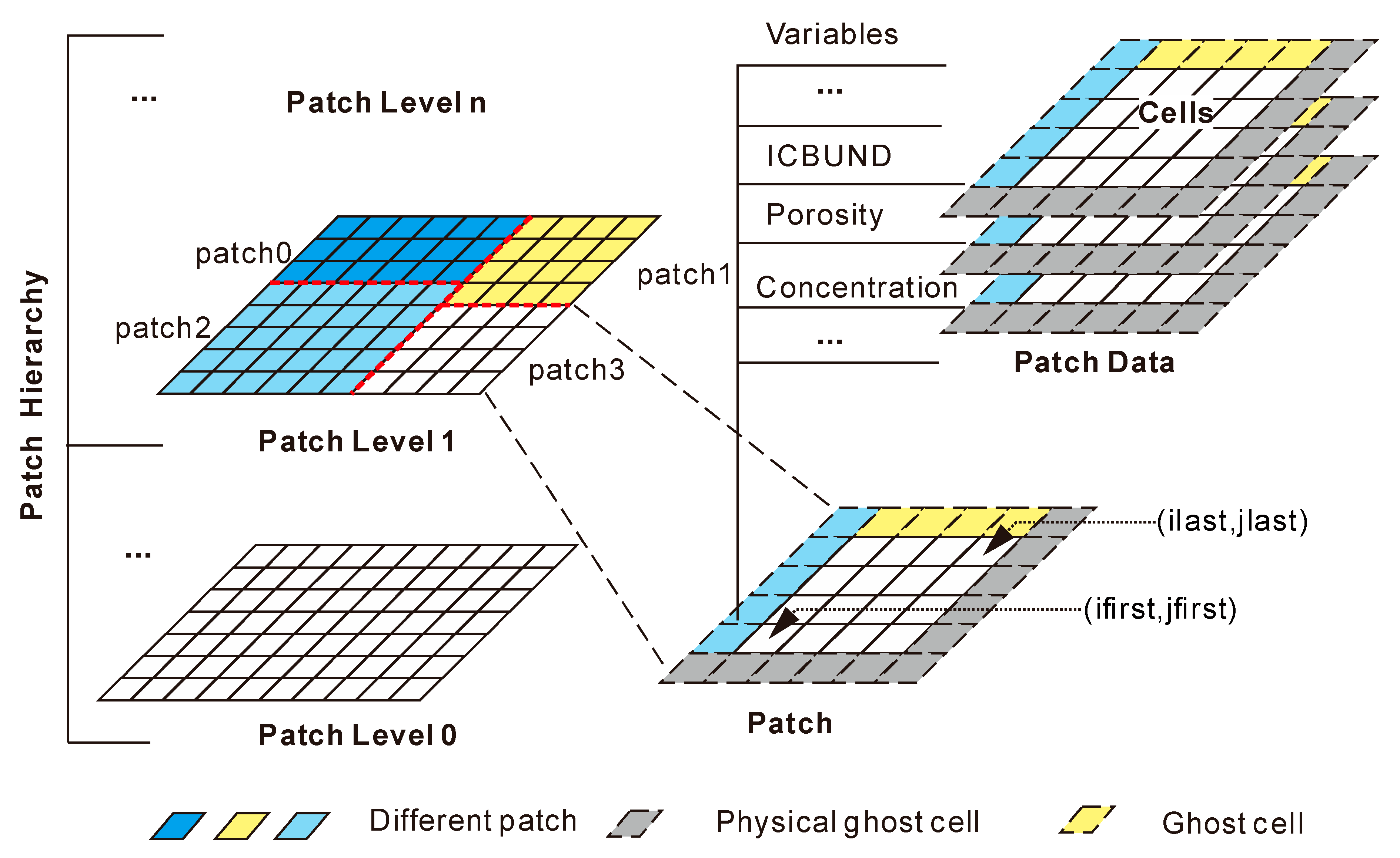
To understand the parallel implementation process, the JASMIN framework is briefly introduced. The JASMIN framework is based on the patch-based data structure of “Patch Hierarchy-Patch Level-Patch-Patch Data-Cells,” which is used to define variables and carry out parallel computing (Figure 1). The patch hierarchy contains multiple patch levels that, can be used to manage patch level reconstruction and refinement. Patch levels consist of non-overlapping patches. As shown in Figure 1, patches contain different patch data (i.e., different variables in programs). In the implementation of parallelization, users need to define only variables on patch data, design parallel algorithms in a simple way, and conduct time integration by adding slight modification to JASMIN-specific data structures. More details about JASMIN can be found in a number of previous studies [24,25,30].
2.3. Parallel Computing Strategies
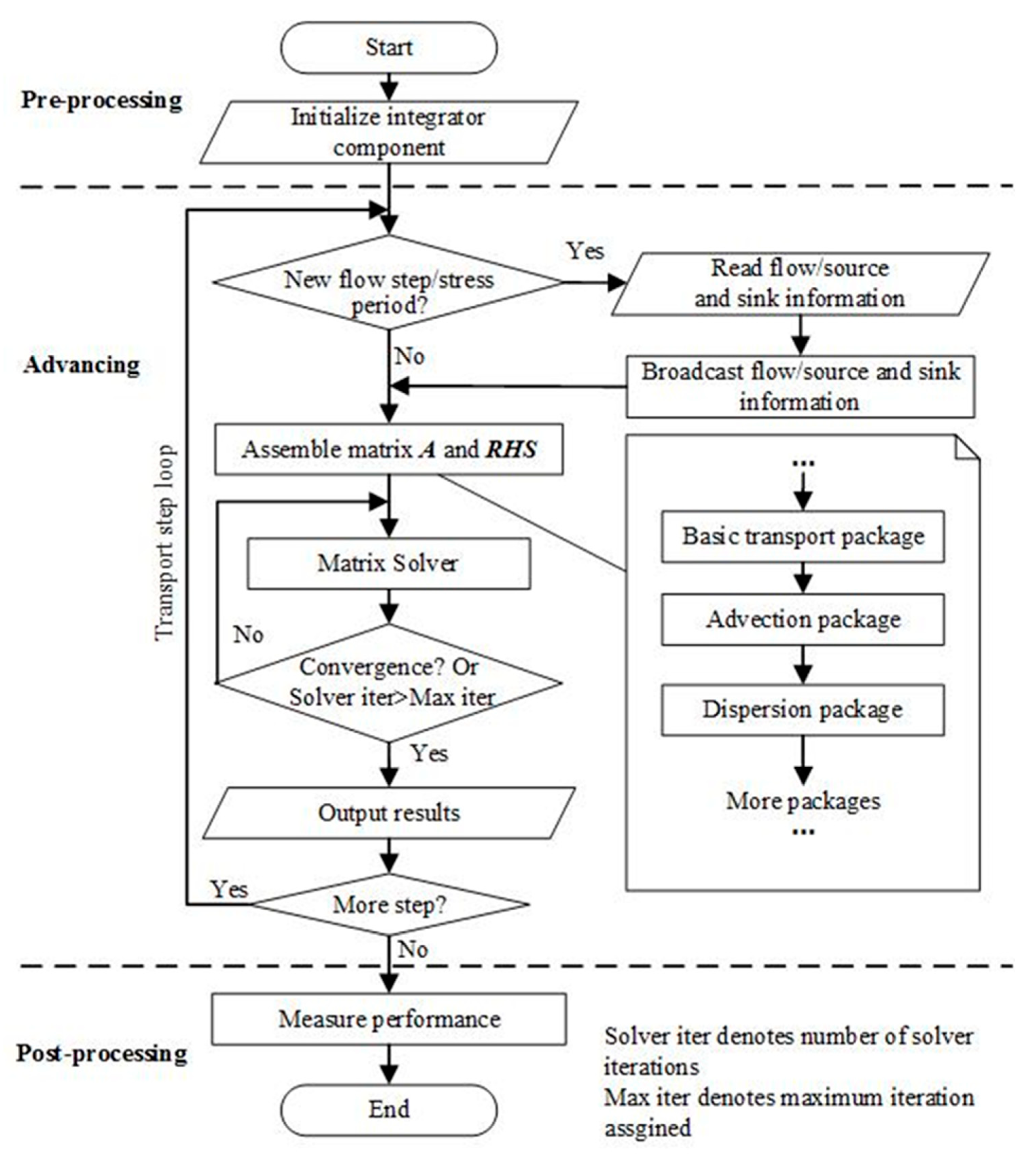
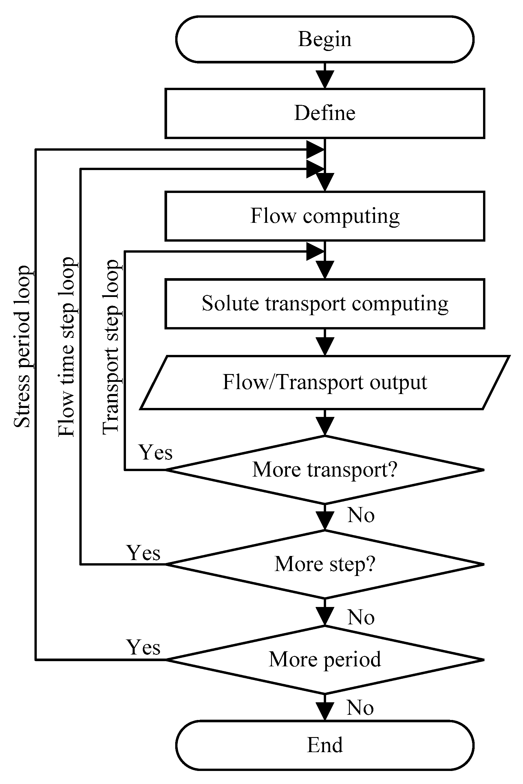
The whole process of JMT3D is similar to MT3DMS. However, these methods have quite different implementations. The flowchart of JMT3D can be divided into three stages—pre-processing, advancing, and post-processing (Figure 2).
In the pre-processing stage, the program mainly accomplishes parallel environment building and data initialization. First, the program initializes the time integrators, which are in charge of data initialization, data replication, numerical calculations, etc. [24], and then builds data structures. Then, the program reads the data from MT3DMS model input files (i.e., .btn, .adv, .ssm, etc. These are input files of MT3DMS. btn stands for basic transport package, adv stands for advection package, ssm stands for the sink & source mixing package) [27] to initialize the patch data (i.e., ICBUND, which indexes specifying the boundary condition type, porosity, starting concentration, etc.) and certain global parameters (i.e., the number of columns, rows, etc.). The patches are then automatically and evenly partitioned to different processors. Global parameters are broadcast to all processors.
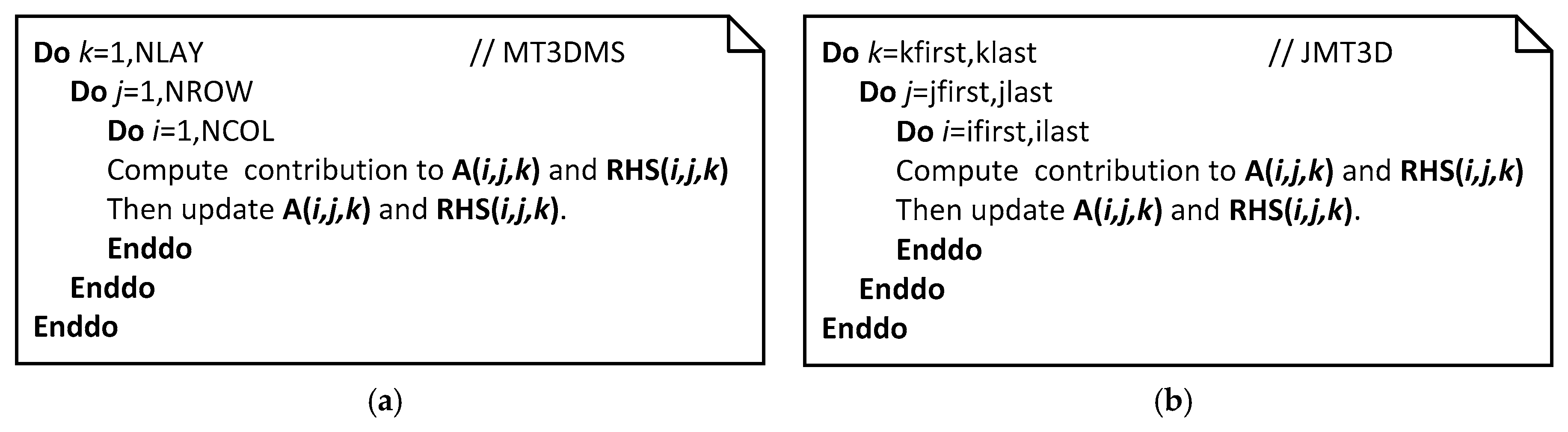
In the advancing stage, the program is mainly responsible for assembling and solving equations (i.e., AX = RHS). The program will initially identify whether the information indicates a new time step or a new stress period of solute. The master processor will read in the flow information and source/sink data and broadcast it to all processors. Next, the program will assemble the coefficient matrix A and RHS depending on different packages via a parallel method. Taking the basic transport package (BTN) as an example, the MT3DMS program loops all columns, rows, and layers in a serial process as shown in Figure 3a. However, this process is inefficient for large models. The JMT3D program is based on patches and loops in the range of patches as shown in Figure 3b. Therefore, different processors can simultaneously perform the assembly of the coefficient matrix of A and RHS.
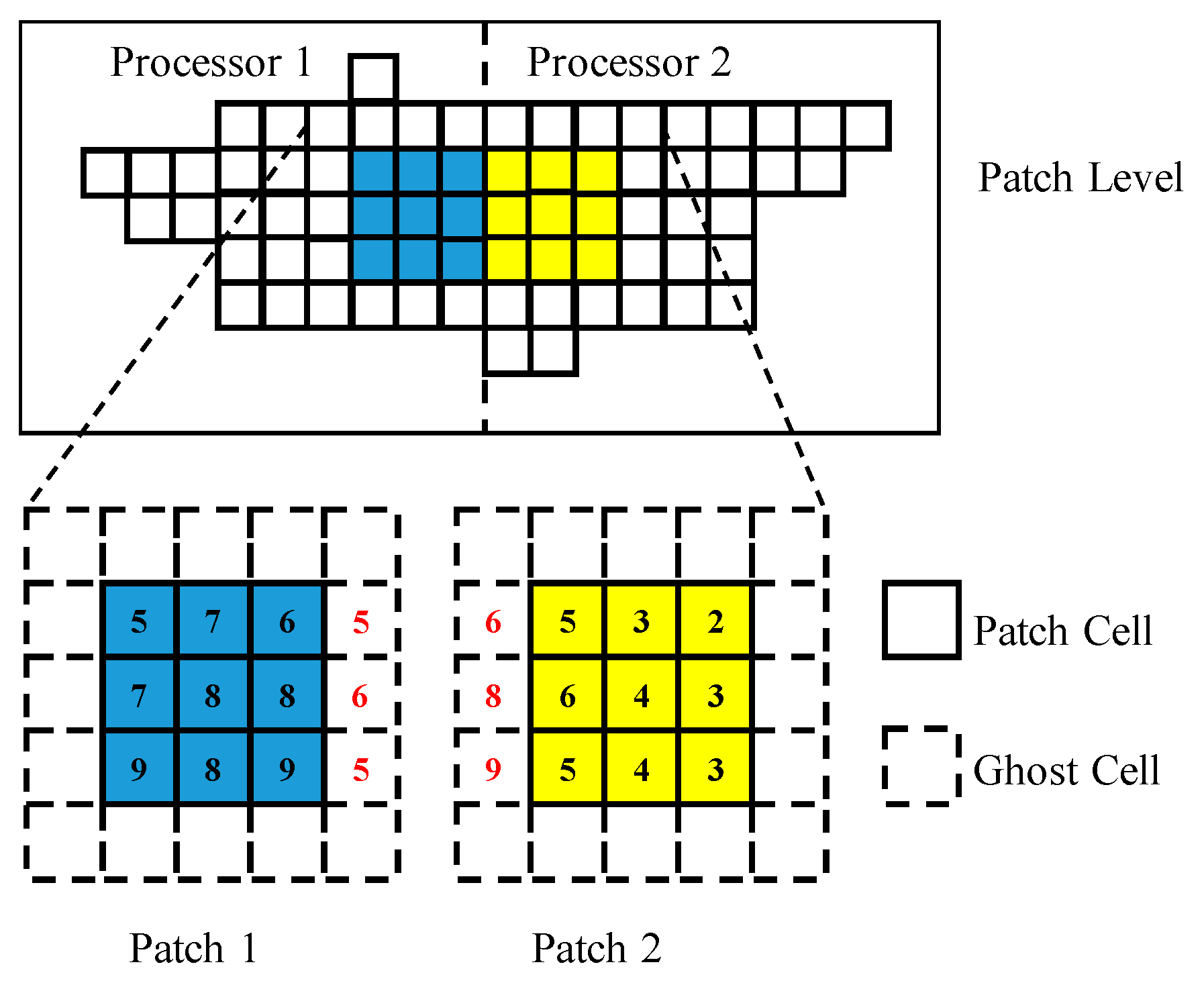
Data communication is required among neighboring patches (processors) for certain packages. For example, assembling equations in a dispersion (DSP) package requires the volumetric flow rates of neighboring cells. The JMT3D program extends each patch to a ghost cell (overlapped with other patches) as shown in Figure 4 by the dashed line. The red numbers of the figure are copied from the cells on the adjacent patch before numerical computing so that each patch can assemble the coefficient matrix A and RHS independently instead of changing information during computation. This approach is called batching the data communication, and it can reduce communication costs and can be highly efficient [25].
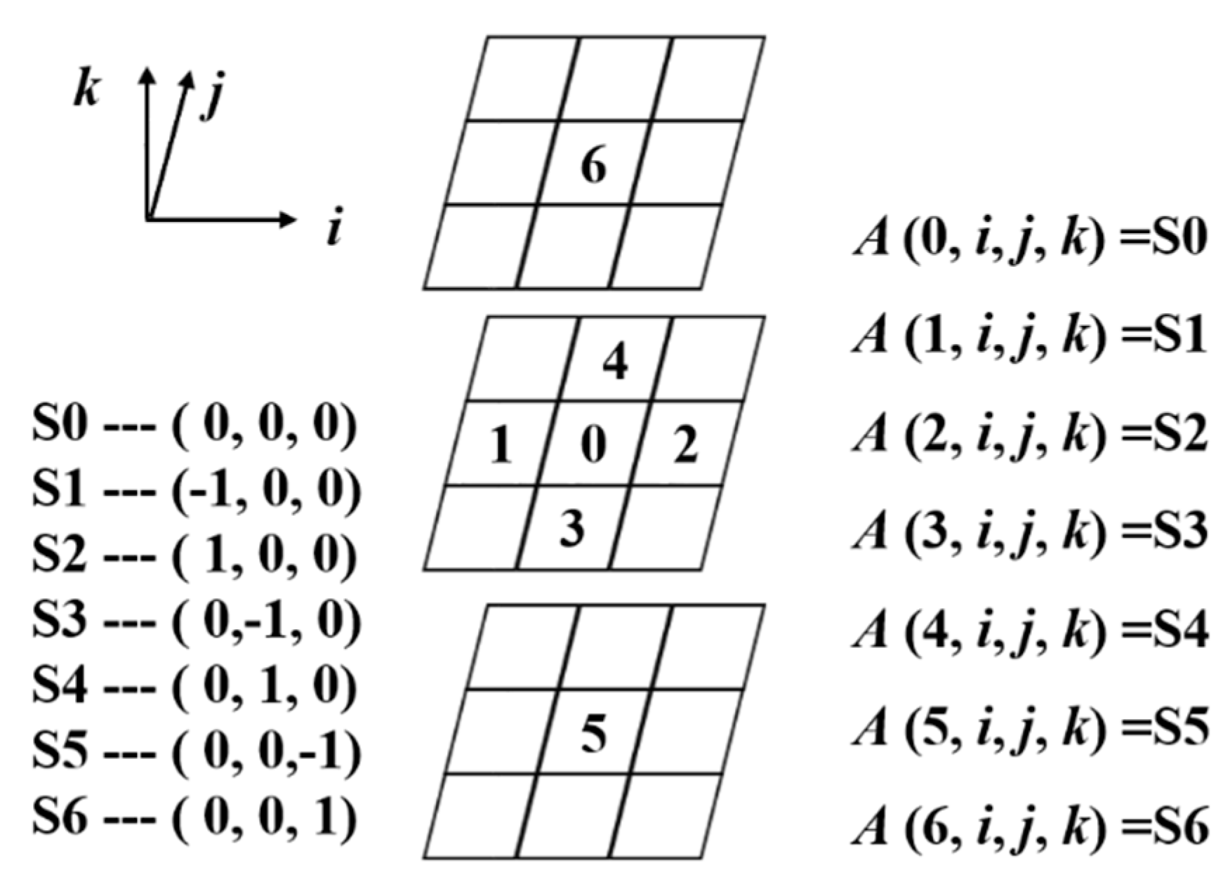
Solving equations is one of the most time-consuming parts of contaminant transport simulation [6]. Therefore, solver methods are significant to parallel performance. The JASMIN framework provides many parallel iterative methods, such as Krylov subspace methods (e.g., CG (conjugate gradient), GMRES (generalized minimal residual algorithm), BiCGSTAB) and preconditioners (e.g., AMG). To conveniently use these methods, a stencil-based is designed for advection-diffusion equation. The stencil-based represents the offset between the stencil component and stencil center (Figure 5). Using the stencil-based method can allow the parallel program to simultaneously solve contaminant transport equations as serial program does, which ensures that the parallel result is consistent with the serial result. When the residual error meets the convergence criterion or exceeds the max iteration number specified by users, the solver stops. Then, the concentration results are outputted.
In the post-processing stage, memory-consumption and time-consumption statistics are outputted in a log file. All types of computing resources are outputted, and the results of the concentration can be visualized by Javis [31].
2.4. Coupling Flow and Solute Simulation
Because MT3DMS needs to read the flow information (i.e., saturated thickness, volumetric flow rates per cell interfaces, etc.) from an intermediate file of the integrated MODFLOW-MT3DMS model, contaminant transport simulations cannot be performed until all flow computing is completed [32]. For a steady flow, the contaminant transport model needs to read only the information of the flow information once. However, for a transient flow, the contaminant transport model needs to read the flow information at each time step. Intermediate files, which store flow information, can become extremely large in large-scale and high-resolution simulation. In addition, reading the intermediate file too frequently will hamper the parallel performance of the program. Therefore, in this study, the MODFLOW-MT3DMS coupling mode was optimized. The JMT3D was enriched by embedding contaminant transport loops into the loop of flow simulation along with the parallel flow simulation program JOGFLOW [25] as shown in Figure 6. The coupled JOGFLOW-JMT3D model can share common variables, such as porosity, layer thickness, etc., as well as internal transport flow information. In addition, the coupled model can output the concentration result immediately after each water flow time step.
3. Results and Discussion
To test the correctness and performance of JMT3D, five types of tests were conducted. First, the correctness of the solution was verified by a transient model. Second, the speedup and memory consumption of different iteration methods were analyzed. Third, the effects of high heterogeneity and transient flow on the performance of the model were tested. Finally, a scaling test with 10 million cells was conducted on dozens to hundreds of processors.
3.1. Correctness Verification
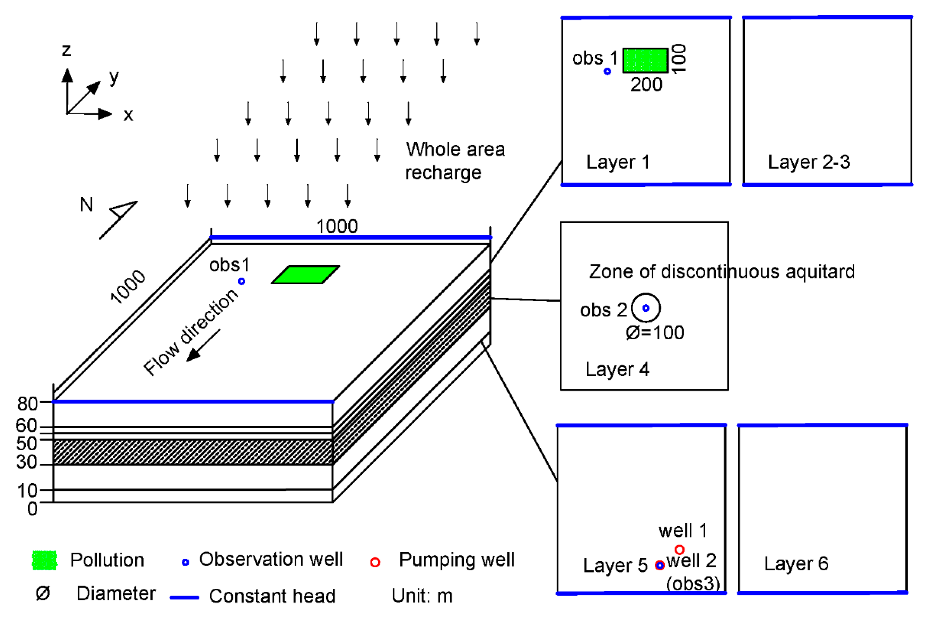
In the correctness verification test, a typical model with three aquifers is designed. The model is composed of an upper sand and gravel aquifer, a lower sand and gravel aquifer, and a middle a clay and silt aquitard with a discontinuous zone in the center of the aquifer. The model is similar to the demo of Waterloo airport in [33]. To increase the accuracy of the computational task, the upper aquifer is divided into three layers, and the lower aquifer is divided into two layers (Figure 7).
The numerical model was simulated using a domain covering an area of 1000 × 1000 m2 with a thickness of 80 m. The problem size can be represented as 20 × 20 × 6 in the x, y, and z directions.
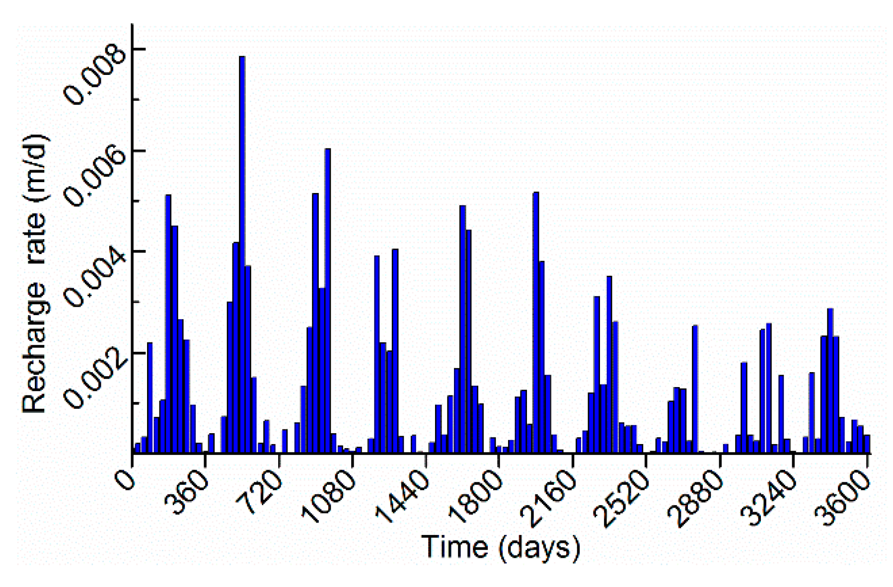
The first layer was defined as an unconfined aquifer, and the others were defined as confined aquifers. Except layer 4, all layers were set as specified heads at the north side (68 m) and south side (70 m). Layer 4 was set no-flow boundary all around. The east and west boundaries of all layers were defined as no-flow boundaries. At the center of the fourth layer, a permeable circular area with a diameter of 100 m is observed, and the center coordinate of the circular area is (500, 500). At the fifth layer, two wells located at (725, 225) and (625, 175) with a rate of −800 m3/d per well. Dynamic recharge occurs at the first layer with the rate in Figure 8. For the contaminant transport model, a rectangular contaminated area with an area of 200 × 100 m2 was located in the first layer. The upper left corner of the rectangular area was located at (400, 900). The contaminant area was treated as initial concentration without other sources. The initial concentration was set to 5000 mg/L. Three observation wells were set at obs 1 (325, 825) in layer 1, obs 2 (525, 475) in layer 4, and obs 3 (625, 175) in layer 5. The model was run for 3600 days with 120 stress periods with one time step per stress period. The contaminant transport program automatically calculates transport steps depending on the flow velocity and Courant number. The others parameters of the flow model and contaminant transport model are shown in Table 1.
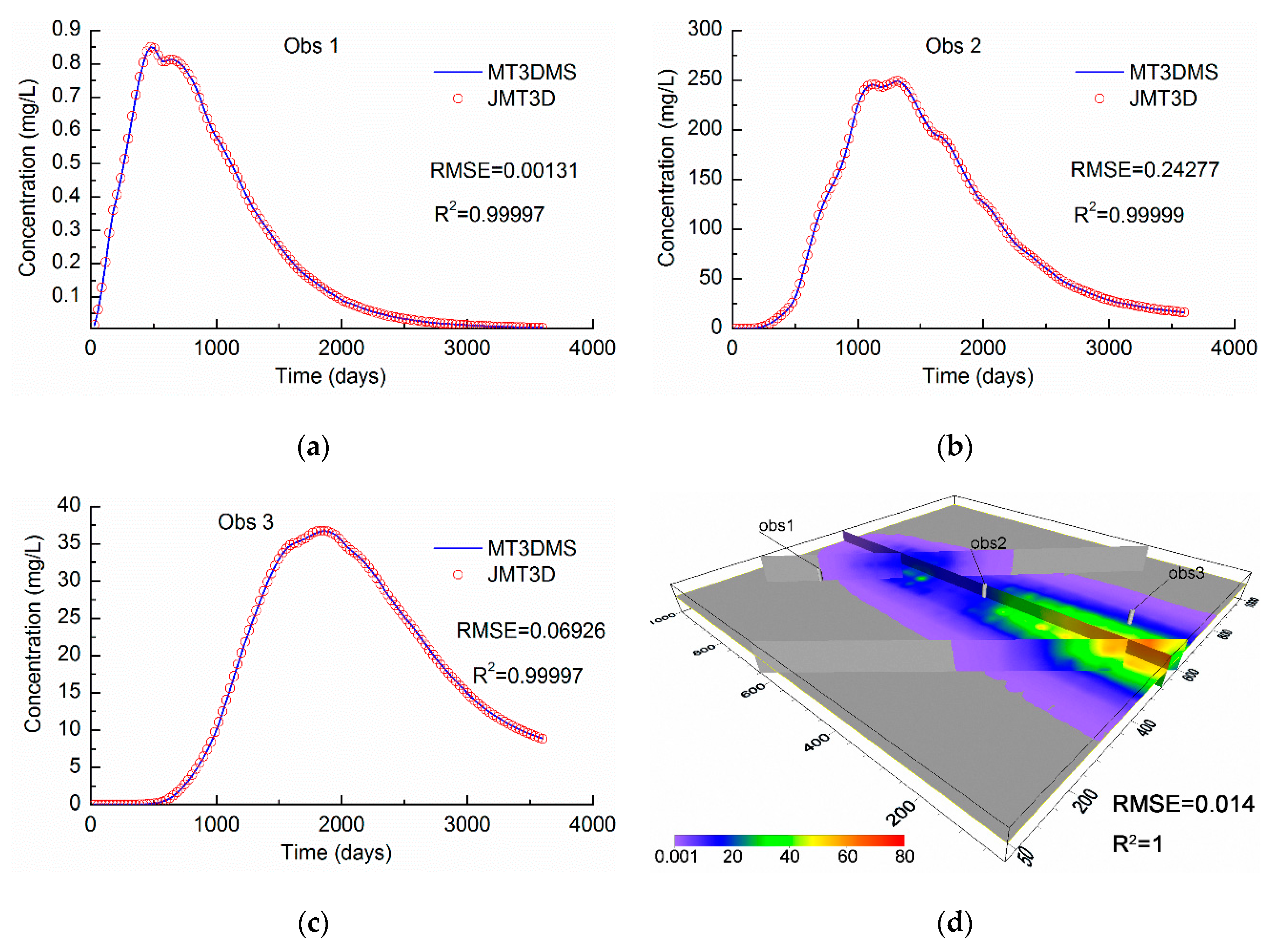
The flow and contaminant transport convergence standard were both set to 1 × 10⁻⁶. The test was carried out on an SR4803S Linux workstation with 4 AMD OPTERON 6174 CPUs (2.2 GHz). Each CPU contained 12 processors, and the memory was 64 GB DDR3. The JASMIN framework version 2.1 (CAEP software center for high performance numerical simulation, Beijing, China) and the visual software JAVIS 1.2.3 (CAEP software center for high performance numerical simulation, Beijing, China) were used. All codes were compiled by GCC 4.5.1 with -O2 flags. The solutions of JMT3D on one processor were compared with numerical solutions of MODFLOW-MT3DMS. The root-mean-square error (RMSE) and the coefficient of determination were used to evaluate the correctness. The smaller the RMSE value, the better the result. The closer the coefficient of determination to 1, the better the result.
where RMSE denotes the root-mean-square error, R2 denotes the coefficient of determination, Ci MT3DMS denotes the concentration of cell i of MT3DMS, Ci JMT3D denotes the concentration of cell i of JMT3D, and denotes the average concentration of MT3DMS or JMT3D.
As shown in Figure 9, all the R2 values of the observation wells are above 0.99. The concentration at 3600 days presents values of RMSE = 0.014 mg/L and R2 = 1, and the average relative error is 1.72 × 10⁻³. These findings show that the results of JMT3D can maintain a small error compared with the original results from the MODFLOW-MT3DMS program. The reason for the error is that JMT3D continues to use the flow information of JOGFLOW. Although the results of JOGFLOW are consistent with the results of MODFLOW [25], it is impossible to guarantee that all flow information is exactly the same. The difference of flow will be transmitted to the contaminant transport computation. A comparison of the higher initial concentration and the final concentration shows that the relative errors ranged from 10−4~10−6, and the accuracy is sufficient to meet the actual need. In our opinion, the result fits well with the MT3DMS. In addition, some tests were conducted to compare the serial with parallel processes. The relative errors between the serial and parallel processes are less than 10−6. The errors are affected only by the rounding error at different core numbers.
3.2. The Parallel Performance with Different Iteration Methods
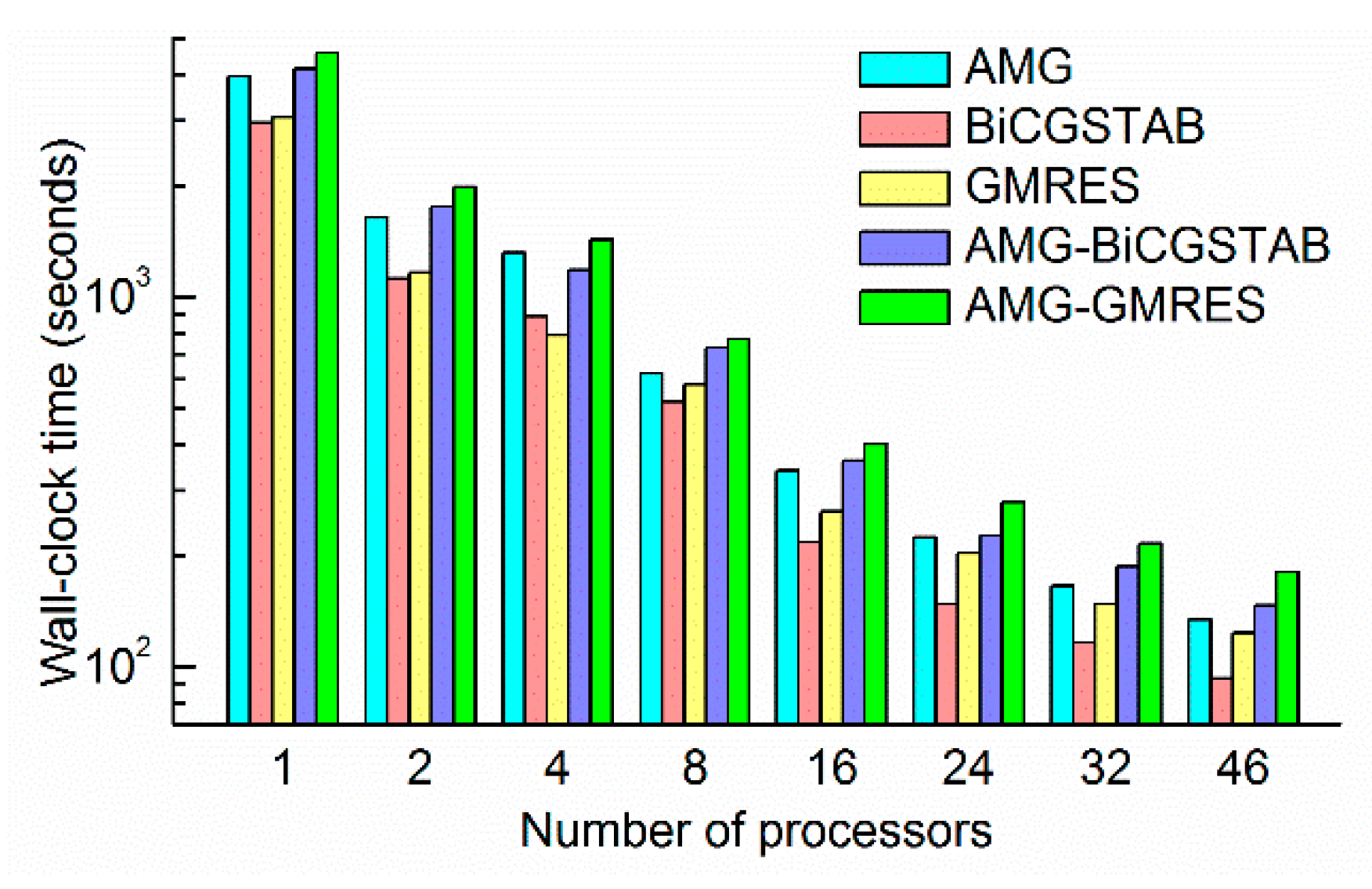
To test the parallel performance of JMT3D, the model for correctness verification was refined 10 times in both the x and y direction. The new problem size can be represented as 200 × 200 × 6 in the x, y, and z directions. The size of each cell is 5 × 5 × N m (N is the thickness of different layers). First, a steady flow was performed, and the rate of recharge was changed to 6 × 10⁻⁴ m/d. The other parameters were unchanged. The flow model was solved by the common CG iteration method. The contaminant transport model was solved by the algebraic multigrid (AMG), Bi-conjugate gradient variant algorithm (BiCGSTAB), generalized minimal residual algorithm (GMRES), BiCGSTAB with preconditioner AMG (AMG-BiCGSTAB), and GMRES with preconditioner AMG (AMG-GMRES) methods. Every method was tested on 1, 2, 4, 8, 16, 24, 32, and 46 processors, respectively. The flow and contaminant transport convergence standard were both set to 1 × 10⁻⁶, and the maximum iteration number was set to 100. To exclude occasional errors, the model was tested at least three times for each method.
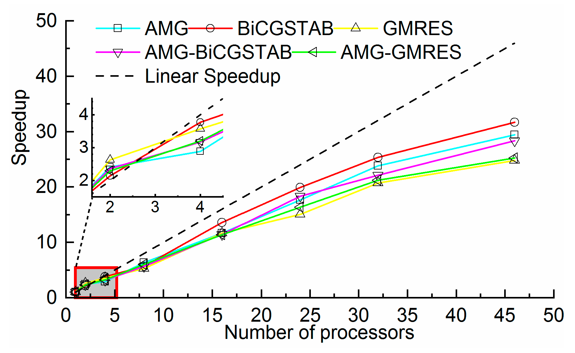
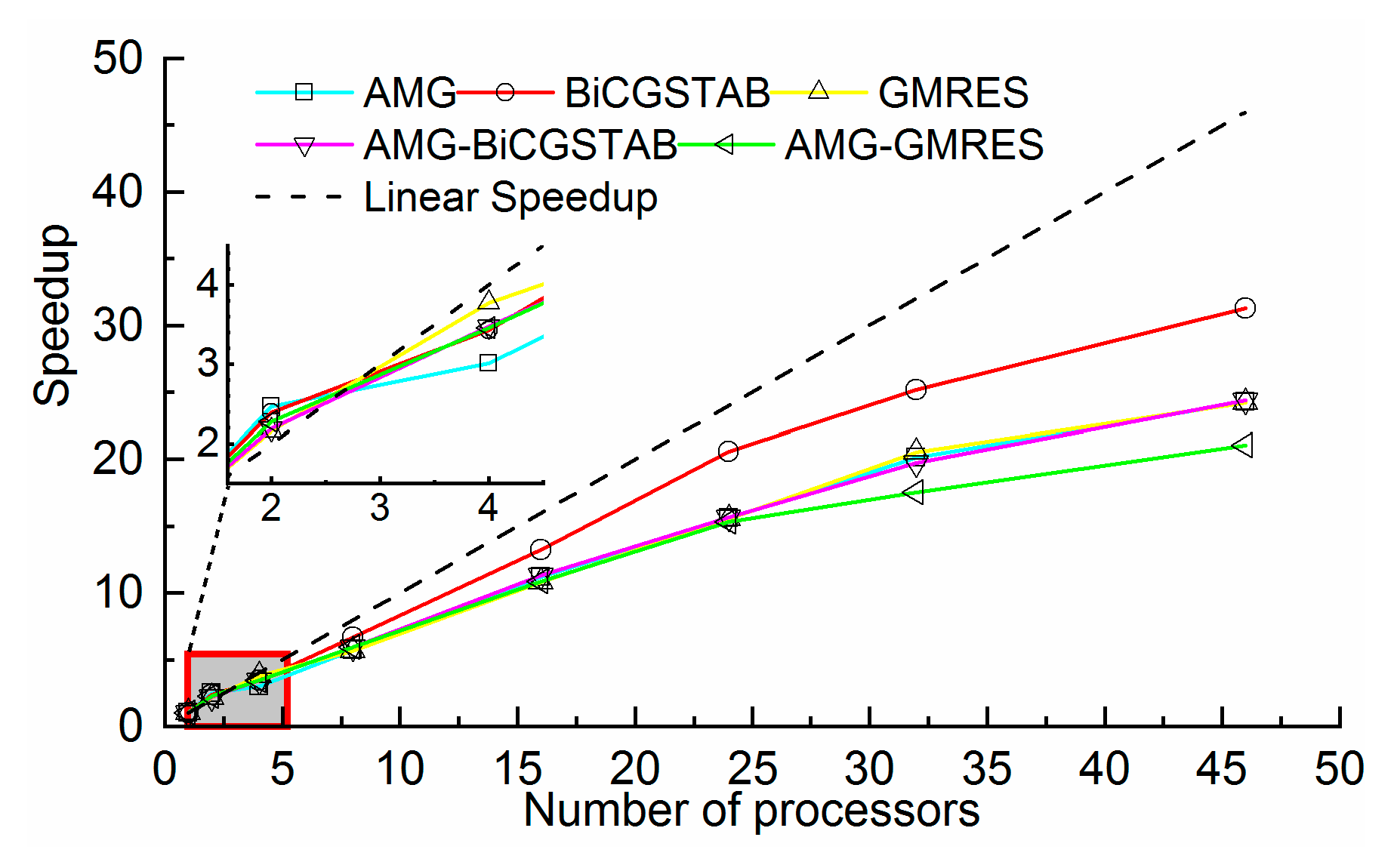
Parallel performance is usually measured by speedup and efficiency [19,34]. Speedup represents the ratio of serial wall-clock time to parallel wall-clock time. Linear speedup represents the ratio of the number of parallel processor to the number of basic processor (in general one). When a speedup is larger than the linear speedup, it is called a super-linear speedup. Efficiency represents the ratio of speedup to the number of processors.
where Sp denotes the speedup, Ts denotes the wall-clock time in the serial program, Tp denotes the wall-clock time in the parallel program, Ep denotes the efficiency of a parallel program, and P denotes the number of processors.
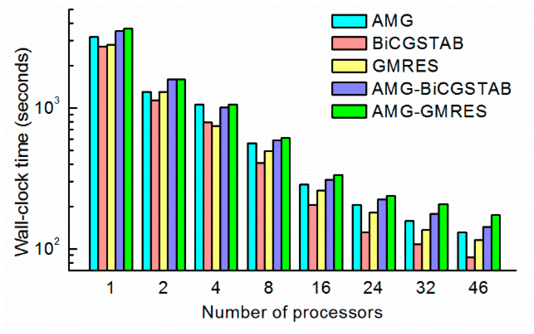
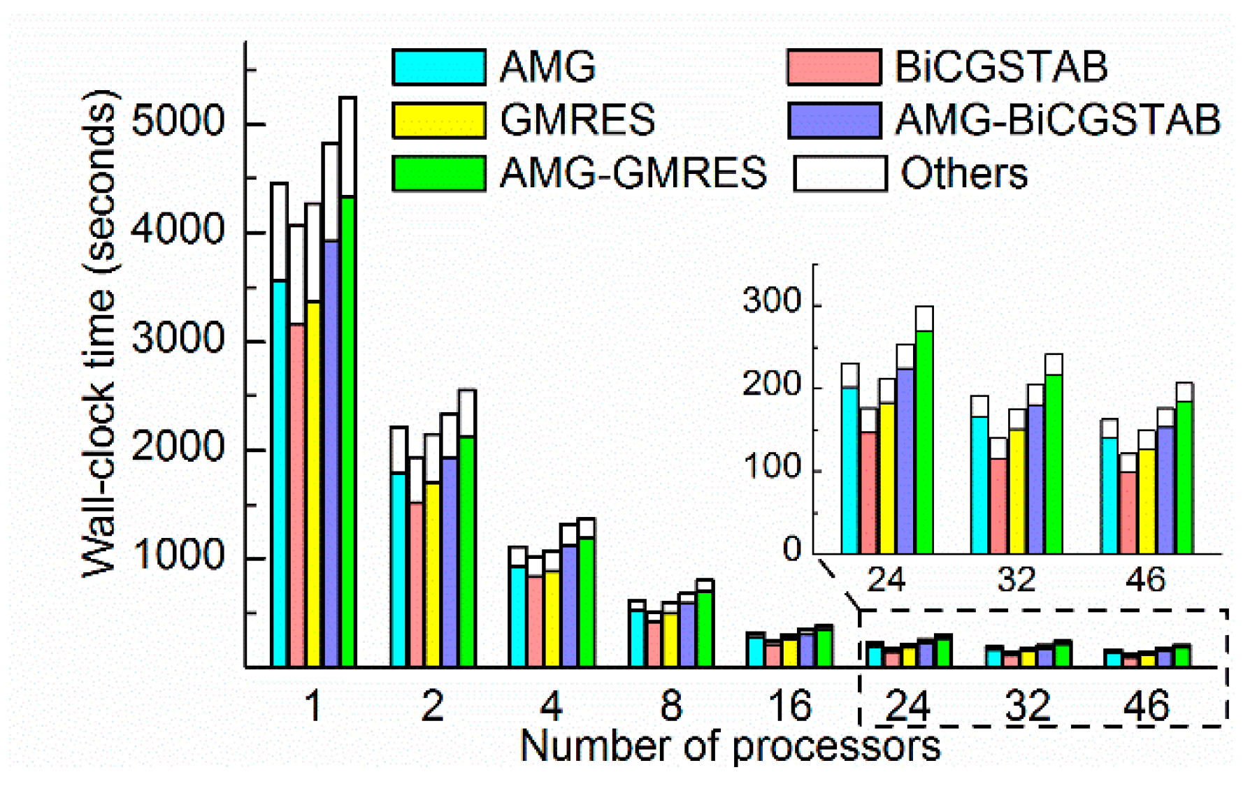
The time-consumption and speedup of each method is shown in Figure 10 and Figure 11. All the wall- clock times were gradually reduced as the number of processors increased. Different methods, even with the same number of processors, required a significantly different amount of time. For example, the AMG-GMRES method required 180 s on 46 processors, where the BiCGSTAB method required only 93 s. These findings demonstrate the importance of choosing a convenient solver method. As shown in Figure 10, the BiCGSTAB method required the least time in most cases. The wall-clock time of BiCGSTAB significantly decreased from 2948 s on one processor to 93 s on 46 processors. The wall-clock time of the GMRES method was slightly lower than that of the BiCGSTAB method with four processors, which indicates that the task of each processor (60 k cells per processor) was more suitable for the GMRES methods. The AMG and AMG as preconditioner methods required more time than the BiCGSTAB and GMRES methods because the AMG required more time for setup and per iteration [35].
As shown in Figure 11, the BiCGSTAB method also achieved high speedups, when the number of processors was greater than 16. A maximum speedup 31.7 was achieved with 46 processors. In addition, all methods achieved super-linear speedup on two processors. The speedup of the GMRES method ranked first with an efficiency of 132%. The reason for the super-linear speedup is that the access data fit in the cache of each processor. The time saved by the cache effect offset the communication overhead time in parallel computing. With an increasing number of processors, the parallel communication overhead increased, and the cache effect became obvious. Although the super-linear speedup disappeared, all the methods achieved a good speedup. The parallel efficiency was between 53% and 132%. Therefore, the JMT3D can effectively reduce the time-consumption and achieve high speedup.
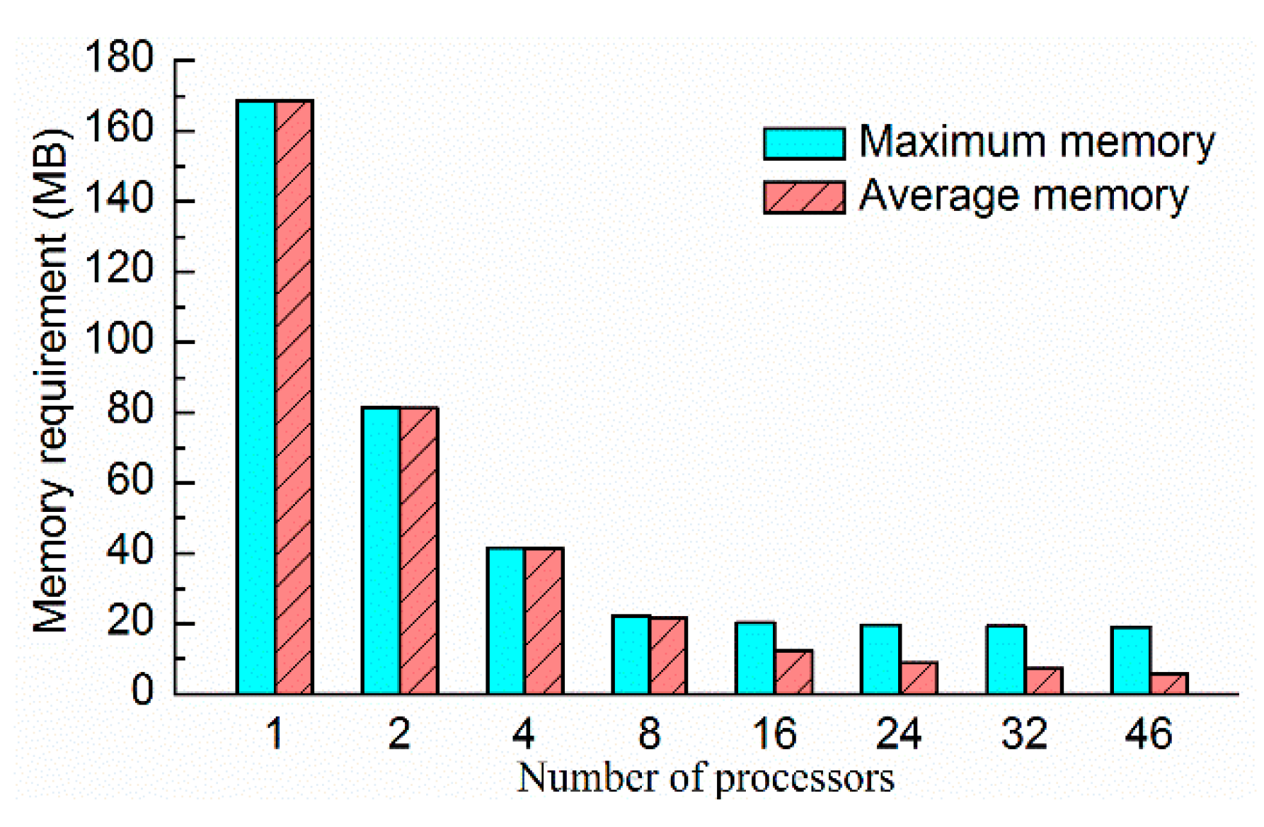
The JMT3D not only reduced the wall-clock time but also reduced the memory consumptions. The memory consumptions of different methods were approximately the same. Taking the AMG method as an example, both the maximum memory consumption and average memory consumption decreased as the number of processors increased. As shown in Figure 12, the maximum memory consumption was reduced significantly from 169 MB on one processor to 22 MB on eight processors. The maximum memory consumption was slightly reduced as the number of processors increased. Memory consumption is related to global variables and various types of objects for framework running. The maximum memory consumption was determined by the master processor because the master processor is in charge of data initialization, reading, and broadcasting source data. Compared with one processor, the maximum memory consumption on 46 processors decreased by 89%, and the average memory consumption on 46 processors decreased by 96%. The results demonstrate that the JMT3D can reduce both the maximum memory consumption and average memory consumption. Reducing the maximum memory consumption can solve the memory consumption bottleneck problem for large-scale simulations, and reducing the average memory consumption can reduce the hardware demands for the non-master processor.
3.3. The Parallel Performance with High Heterogeneity
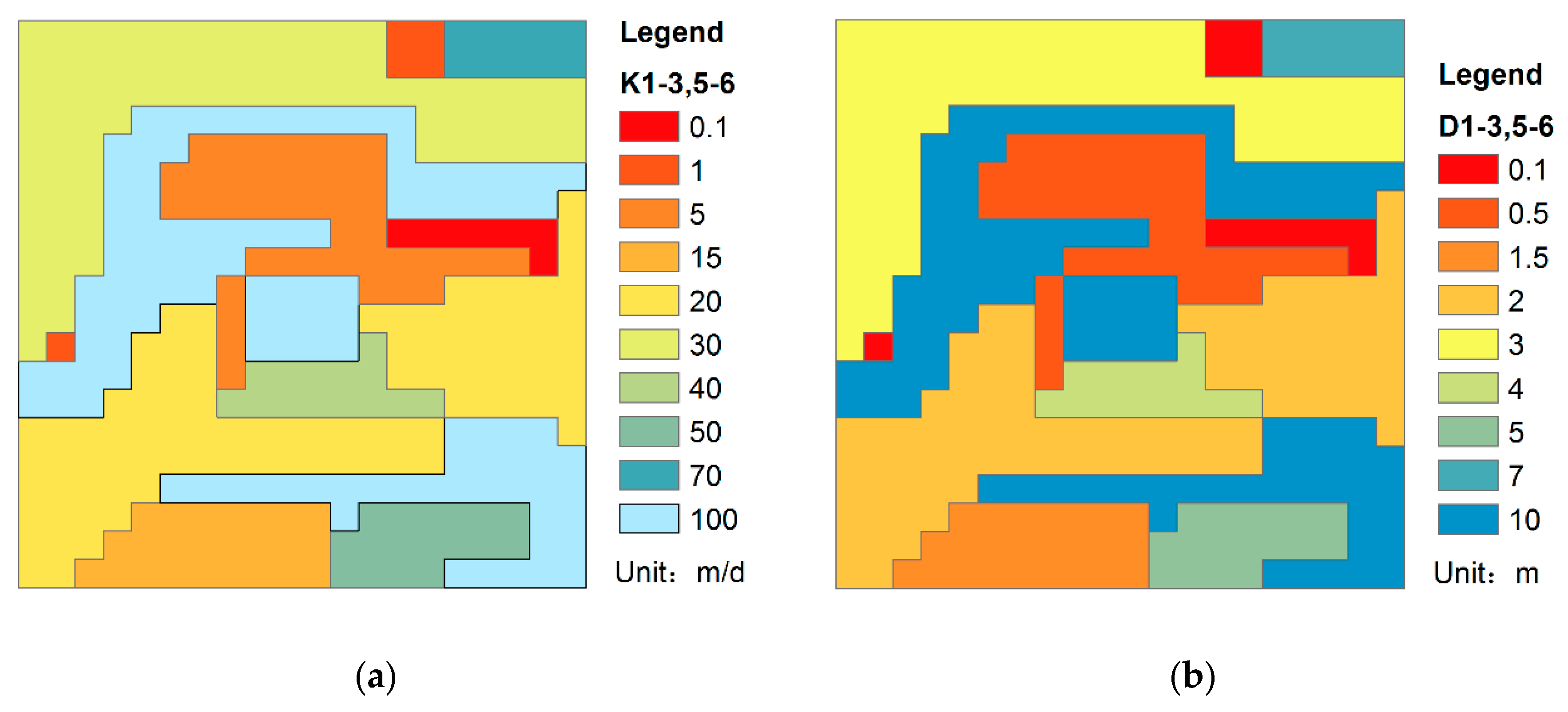
Heterogeneity usually exists in the study areas and affects contaminant transport. To determine whether heterogeneity will affect parallel performance, random hydraulic conductivity and longitudinal dispersion area were constructed. Except for the fourth level (silt aquitard), all the layers were set as shown Figure 13. The other parameters were the same as the model in Section 3.2.
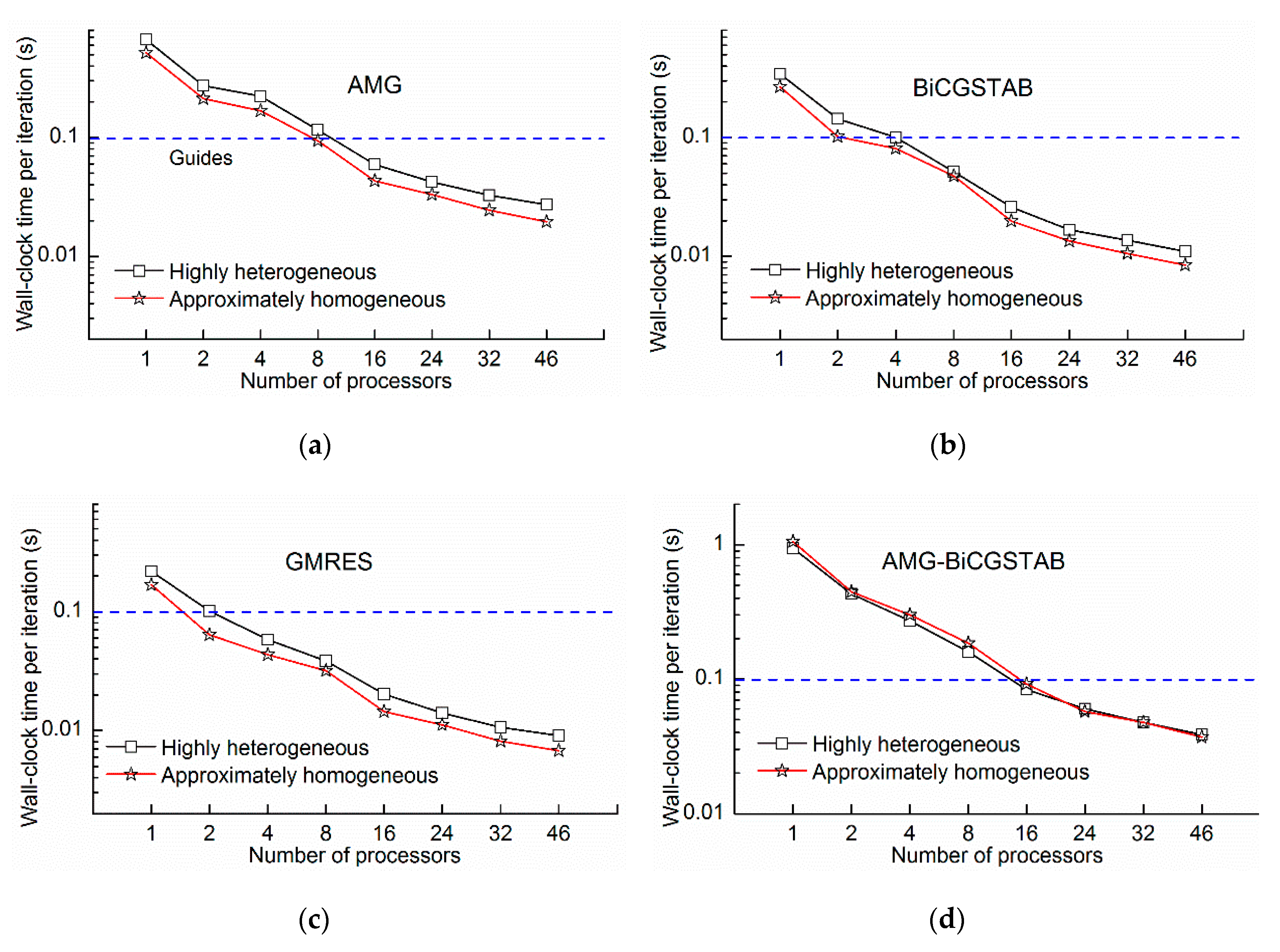
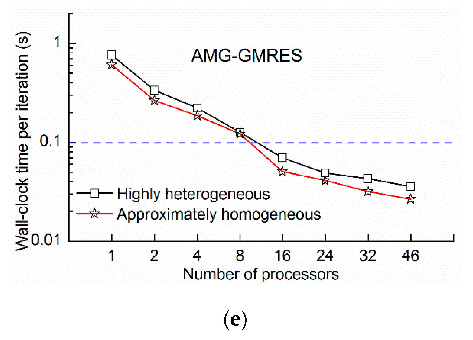
To facilitate the analysis, the model in Section 3.2 is called the approximately homogeneous model, and the model in this section is called the highly heterogeneous model. As shown in Figure 14, the wall-clock times of the highly heterogeneous model were lower than those of the approximately homogeneous model because the transport step of highly heterogeneous model was 0.97 days compared with the 0.91 days of the approximately homogeneous model, and the number of transport steps decreased. The phenomenon was extensively analyzed by the wall-clock time per iteration. As shown in Figure 15, the wall-clock times per iteration of the highly heterogeneous model were generally higher than those of the approximately homogeneous model. Due to heterogeneity, the solver does not converge easily. However, the wall-clock time per iteration of the AMG-BiCGSTAB method is almost unchanged for both the highly heterogeneous model and the approximately homogeneous model, which indicated that the AMG-BiCGSTAB model was less affected by heterogeneity.
The GMRES method required the least time per iteration (Figure 15); however, the convergence of the GMRES was not as good as the other solutions, and it presented the highest number of iterations (Table 2). Moreover, the number of iterations of BiCGSTAB and GMRES with AMG as the preconditioner was significantly reduced, indicating that AMG improved the convergence abilities of the BiCGSTAB and GMRES method. The iterations of different methods with different numbers of processors remained almost unchanged (Table 2). The contaminant transport equations should be solved simultaneously by using the stencil-based method. The stencil-based method and domain decomposition method can ensure that the solution accuracy and convergence do not decrease as the number of domains increase, thereby maintaining as much consistency in the results as possible. The difference in the number of iterations of the AMG method was caused by rounding errors on different processors. The greatest difference in the number of iterations was smaller than 2%, which is inconsistent with previous work, which iterations increased with increasing numbers of processors [6,19].
As shown in Figure 16, all the methods achieved super-linear speedup on the two processors. The BiCGSTAB method achieved the largest speedup of 31.3 on 46 processors and presented an efficiency of 68%, and its speedup ranked first on 8, 16, 24, 32, and 46 processors. The speedups of other methods were approximately similar. These results indicate that the heterogeneity had little effect on the speedup performance of JMT3D.
3.4. The Parallel Performance with Transient Flow
To address concern related to the effect of transient flows on performance, the highly heterogeneous steady flow model in Section 3.3 was changed to a transient flow model. The dynamic recharge and stress periods were the same as that of the model in Section 3.1. All other parameters were unchanged.
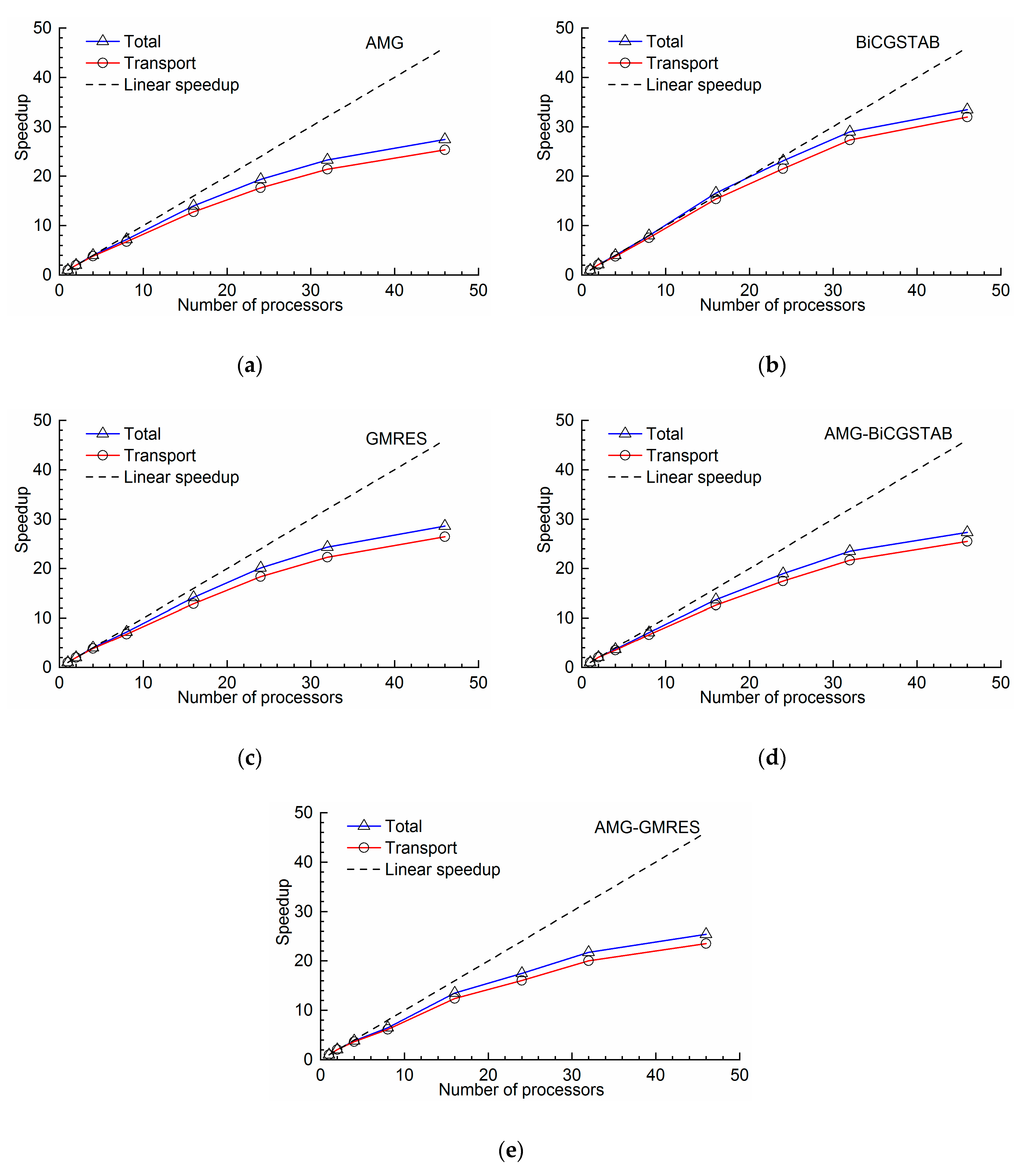
The wall-clock time of contaminant transport and the total wall-clock time (the sum of contaminant transport and others) are shown in Figure 17. The wall-clock time of contaminant transport accounted for the greatest amount of total wall-clock time (from approximately 80% on one processor to approximately 90% on 46 processors), because the transport step length is automatically reduced with the limit of the Courant number; and a flow time step is refined into more transport steps [2]. For example, the flow time step is 30 days in this model. To guarantee a value of Courant = 1, the transport step length was adjusted to 0.009~0.28 days depending on the velocity of flow. In the high-resolution contaminant transport simulation, the smaller the mesh size, the shorter the length of transport step. Therefore, solving contaminant transport effectively is the key to performing high-resolution simulation of integrated flow and containment transport.
The speedups of total and contaminant transport were shown in Figure 18. It shows that the total speedup of each method is better than that of contaminant transport. A further detailed analysis of the wall-clock time of each part was conducted. Using the BiCGSTAB method as an example (Table 3), the flow and contaminant transport account for the major percentage of wall-clock time. The share of flow decreased; and the share of other components slightly increased as the number of processors increased because non-parallel parts, such as initialization and reading recharge sources, exist in the program. These non-parallel parts run in serial and require a constant time. When the total wall-clock time decreases, the proportion of these parts increases. The acceleration of the flow part improved the total speedup. Coupling the flow and contaminant transport in parallel can further increase the parallel efficiency. For example, the BiCGSTAB method achieved remarkable speedup (i.e., 33.45 for the total progress, and 31.98 for the contaminant transport part on 46 processors) (Figure 18). In addition, the flow and solute results can be outputted instantly without waiting for the computation of all periods of flow to be finished, which is of great significance to the online simulation system.
3.5. Scaling Tests
Scaling tests can be used to evaluate the abilities of parallel programs, and provide the optimal number of processors on a certain type of parallel machine. The performance on a larger processor can be predicted based on the parallel performance of the program on a small scale processor. In this study, strong scalability (the problem size remains fixed as the number of processors increase) [19] was used to evaluate the performance of JMT3D. The highly heterogeneous model in Section 3.3 was refined eight times in both the x and y directions. The new model size was fixed to 1600 × 1600 × 6. When the cell size is small, the length of the per transport step changes to 0.08 days with the limitation of the Courant number. The results show that the transport step shortens when the resolution increase. Considering the limitation of computer runtime and testing purposes, 1000 transport steps were performed. Moreover, to ensure that most areas presented concentrations, the concentrations of the 1500th day in the heterogeneous model of the transient flow in Section 3.4 were used as the initial concentrations. The flow was set to a steady flow in this model. The wall-clock time of flow was less than 1%, which can be disregarded. The test was performed on a petascale supercomputer at the High-Performance Computing Center of the Institute of Applied Physics and Computational Mathematics in Beijing, China. The AMG and BiCGSTAB methods were used to solve the problem on 28, 56, 112, and 224 processors.
As shown in Table 4, the wall-clock time reduced as the number of processors increased. The BiCGSTAB method achieved the global minimum wall-clock time (516 s) on 224 processors and required less time than the AMG method on a different number of processors. The wall-clock time of AMG method was 2.6 times greater than that of the BiCGSTAB method on 28 processors, which shows that choosing an appropriate method is very important. Although the AMG method required more time, it showed a remarkable scalability in this test and achieved more than 100% efficiency on 112 and 224 processors. The BiCGSTAB method can also achieve good efficiency above 50% on hundreds of processors. The number of iterations of BiCGSTAB was approximately 2.5 times that of the AMG method, which indicates that the AMG method had a better convergence ability than the BiCGSTAB method. The iteration number of different methods on different processors was still unchanged, which demonstrates that the solution accuracy and convergence do not decrease as the region increases. The average consumed memory showed that JMT3D reduced the memory consumption by 80%.
TA and TB denote the wall-clock time of the AMG and BiCGSTAB methods, respectively. EA and EB denote the efficiency of the AMG and BiCGSTAB methods, respectively. IA and IB denote the number of iterations of the AMG and BiCGSTAB methods, respectively.
4. Summary and Outlook
In this study, the high-performance parallel framework JASMIN was used to reconstruct the MT3DMS. To domain decomposition method, ghost cells communication strategy, and stencil-based method were designed and implemented. The flow and contaminant transport simulation were parallel coupled. Then, the developed parallel code JMT3D was verified and tested for correctness and parallel performance using five types of models.
The main contribution and conclusion of this paper are summarized as follows:
- The MT3DMS was parallelized by a high-performance parallel framework, and models with hundreds of thousands to tens of millions of cells were simulated on tens to hundreds of processors. The developed parallel JMT3D speeded up 31.7 times and reduced memory consumption by 96% on 46 processors.
- A domain decomposition method and stencil-based method were implemented. Equations can be solved simultaneously as a serial program. The number of iterations does not increase as the number of processors. This can ensure that results from serial and parallel are as consistent as possible.
- The test results showed that the BiCGSTAB method required the least time and achieved high speedup in most cases. Highly heterogeneity and transient flow have little effect on the speedups. The parallel coupling flow and contaminant transport can further improve the parallel performance, which achieved a 33.45 times greater speedup on 46 processors.
- Contaminant transport simulation is the main time-consuming component of high-resolution flow and contaminant transport simulation. The higher the resolution, the greater the proportion of the contaminant transport simulation.
In the next study, chemical reaction modules will be added into JMT3D, and the load balancing strategy for irregular study areas will be considered in realistic problems.
Author Contributions
Q.Z. and X.L. proposed and designed the research. X.L. and T.C. developed the methodology, conducted the experiments, performed the formal analysis. T.C. and Q.Z. provided the computing resources and fundings. All authors made fairly equal contributions to the writing of the paper. All authors have read and agreed to the published version of the manuscript.
Funding
This research was funded by the special foundation for the basic resources survey program of the ministry of science and technology, China, Grant No. 2017FY100405, and the Natural Science Foundation of China under Grant No. 61602047.
Conflicts of Interest
The authors declare no conflict of interest.
References
- Wheeler, M.F.; Peszynska, M. Computational engineering and science methodologies for modeling and simulation of subsurface applications. Adv. Water Resour. 2002, 25, 1147–1173. [Google Scholar] [CrossRef]
- Zheng, C.M.; Bennett, G.D. Applied Contaminant Transport Modeling, 2nd ed.; Wiley-Interscience: New York, NY, USA, 2002; pp. 273–282. [Google Scholar]
- Hammond, G.E.; Lichtner, P.C. Field-scale model for the natural attenuation of uranium at the Hanford 300 Area using high-performance computing. Water Resour. Res. 2010, 46, 389–390. [Google Scholar] [CrossRef]
- Gwo, J.P.; D’Azevedo, E.F.; Frenzel, H.; Mayes, M.; Yeh, G.T.; Jardine, P.M.; Salvage, K.M.; Hoffman, F.M. HBGC123D: A high-performance computer model of coupled hydrogeological and biogeochemical processes. Comput. Geosci. 2001, 27, 1231–1242. [Google Scholar] [CrossRef]
- Dong, Y.; Li, G. A parallel PCG solver for MODFLOW. Groundwater 2009, 47, 845–850. [Google Scholar] [CrossRef] [PubMed]
- Hwang, H.T.; Park, Y.J.; Sudicky, E.A.; Forsyth, P.A. A parallel computational framework to solve flow and transport in integrated surface-subsurface hydrologic systems. Environ. Model. Softw. 2014, 61, 39–58. [Google Scholar] [CrossRef]
- Abdelaziz, R.; Le, H.H. MT3DMSP - A parallelized version of the MT3DMS code. J. Afr. Earth Sci. 2014, 100, 1–6. [Google Scholar] [CrossRef]
- Wu, Y.S.; Zhang, K.N.; Ding, C.; Pruess, K.; Elmroth, E.; Bodvarsson, G.S. An efficient parallel-computing method for modeling nonisothermal multiphase flow and multicomponent transport in porous and fractured media. Adv. Water Resour. 2002, 25, 243–261. [Google Scholar] [CrossRef]
- Kollet, S.J.; Maxwell, R.M. Integrated surface-groundwater flow modeling: A free-surface overland flow boundary condition in a parallel groundwater flow model. Adv. Water Resour. 2006, 29, 945–958. [Google Scholar] [CrossRef] [Green Version]
- Kollet, S.J.; Maxwell, R.M.; Woodward, C.S.; Smith, S.; Vanderborght, J.; Vereecken, H.; Simmer, C. Proof of concept of regional scale hydrologic simulations at hydrologic resolution utilizing massively parallel computer resources. Water Resour. Res. 2010, 46, W04201. [Google Scholar] [CrossRef]
- Zhang, K.; Wu, Y.-S.; Pruess, K. User’s Guide for TOUGH2-MP-a Massively Parallel Version of the TOUGH2 Code; Report LBNL-315E; Lawrence Berkeley National Laboratory: Berkeley, CA, USA, 2008. [Google Scholar]
- Wei, X.; Li, W.; Tian, H.; Li, H.; Xu, H.; Xu, T. THC-MP: High performance numerical simulation of reactive transport and multiphase flow in porous media. Comput. Geosci. 2015, 80, 26–37. [Google Scholar] [CrossRef]
- Tang, G.; D’Azevedo, E.F.; Zhang, F.; Parker, J.C.; Watson, D.B.; Jardine, P.M. Application of a hybrid MPI/OpenMP approach for parallel groundwater model calibration using multi-core computers. Comput. Geosci. 2010, 36, 1451–1460. [Google Scholar] [CrossRef]
- Mahinthakumar, G.; Saied, F. A hybrid MPI-OpenMP implementation of an implicit finite-element code on parallel architectures. Int. J. High Perform. Comput. Appl. 2002, 16, 371–393. [Google Scholar] [CrossRef]
- Le, P.V.V.; Kumar, P. Interaction between ecohydrologic dynamics and microtopographic variability under climate change. Water Resour. Res. 2017, 53, 8383–8403. [Google Scholar] [CrossRef]
- Le, P.V.V.; Kumar, P.; Valocchi, A.J.; Dang, H.-V. GPU-based high-performance computing for integrated surface-sub-surface flow modeling. Environ. Model. Softw. 2015, 73, 1–13. [Google Scholar] [CrossRef] [Green Version]
- Ji, X.; Li, D.; Cheng, T.; Wang, X.-S.; Wang, Q. Parallelization of MODFLOW using a GPU library. Groundwater 2014, 52, 618–623. [Google Scholar] [CrossRef] [PubMed]
- Miller, C.T.; Dawson, C.N.; Farthing, M.W.; Hou, T.Y.; Huang, J.; Kees, C.E.; Kelley, C.T.; Langtangen, H.P. Numerical simulation of water resources problems: Models, methods, and trends. Adv. Water Resour. 2013, 51, 405–437. [Google Scholar] [CrossRef]
- Hammond, G.E.; Lichtner, P.C.; Mills, R.T. Evaluating the performance of parallel subsurface simulators: An illustrative example with PFLOTRAN. Water Resour. Res. 2014, 50, 208–228. [Google Scholar] [CrossRef] [Green Version]
- SAMRAI: Structured Adaptive Mesh Refinement Application Infrastructure. Available online: http://computation.llnl.gov/projects/samrai (accessed on 9 April 2020).
- Benzi, M. Preconditioning techniques for large linear systems: A survey. J. Comput. Phys. 2002, 182, 418–477. [Google Scholar] [CrossRef] [Green Version]
- PESTc. Available online: http://www.mcs.anl.gov/petsc/index.html (accessed on 9 April 2020).
- MacNeice, P.; Olson, K.M.; Mobarry, C.; De Fainchtein, R.; Packer, C. PARAMESH: A parallel adaptive mesh refinement community toolkit. Comput. Phys. Commun. 2000, 126, 330–354. [Google Scholar] [CrossRef] [Green Version]
- Mo, Z.; Zhang, A.; Cao, X.; Liu, Q.; Xu, X.; An, H.; Pei, W.; Zhu, S. JASMIN: A parallel software infrastructure for scientific computing. Front. Comput. Sci. China 2010, 4, 480–488. [Google Scholar] [CrossRef]
- Cheng, T.; Mo, Z.; Shao, J. Accelerating groundwater flow simulation in MODFLOW using JASMIN-Based parallel computing. Groundwater 2014, 52, 194–205. [Google Scholar] [CrossRef] [PubMed]
- Cheng, T.; Shao, J.; Cui, Y.; Mo, Z.; Han, Z.; Li, L. Parallel simulation of groundwater flow in the North China Plain. J. Earth Sci.-China 2014, 25, 1059–1066. [Google Scholar] [CrossRef]
- Zheng, C.; Wang, P.P. MT3DMS: A Modular Three-Dimensional Multispecies Transport Model for Simulation of Advection, Dispersion, and Chemical Reactions of Contaminants in Groundwater Systems. In Documentation and User’s Guide; Alabama University: Tuscaloosa, AL, USA, 1999. [Google Scholar]
- Ehtiat, M.; Mousavi, S.J.; Srinivasan, R. Groundwater modeling under variable operating conditions using SWAT, MODFLOW and MT3DMS: A catchment scale approach to water resources management. Water Resour. Manag. 2018, 32, 1631–1649. [Google Scholar] [CrossRef]
- Hecht-Mendez, J.; Molina-Giraldo, N.; Blum, P.; Bayer, P. Evaluating MT3DMS for heat transport simulation of closed geothermal systems. Ground Water 2010, 48, 741–756. [Google Scholar] [CrossRef] [PubMed]
- Cao, X.; Mo, Z.; Liu, X.; Xu, X.; Zhang, A. Parallel implementation of fast multipole method based on JASMIN. Sci. China-Inf. Sci. 2011, 54, 757–766. [Google Scholar] [CrossRef]
- Xiao, L.; Cao, X.; Cao, Y.; Ai, Z.; Xu, P. Efficient coupling of parallel visualization and simulations on tens of thousands of cores. In Proceedings of the International Conference on Virtual Reality and Visualization, Beijing, China, 4–5 November 2011. [Google Scholar] [CrossRef]
- Zheng, C.; Hill, M.C.; Hsieh, P.A. MODFLOW-2000, the US Geological Survey Modular Ground-Water Model: User Guide to the LMT6 Package, the Linkage with MT3DMS for Multi-Species Mass Transport Modeling (No. 2001–2082); USGS: Denver, CO, USA, 2001. [Google Scholar]
- Guiguer, N.; Franz, T. Visual MODFLOW, User’s Manual; Waterloo hydrogeologic Inc.: Waterloo, ON, Canada, 1996. [Google Scholar]
- Amdahl, G.M. Validity of the single processor approach to achieving large scale computing capabilities. In Proceedings of the spring joint computer conference, Atlantic City, NJ, USA, 18–20 April 1967; ACM: New York, NY, USA, 1967; pp. 483–485. [Google Scholar] [CrossRef]
- Ghai, A.; Lu, C.; Jiao, X. A comparison of preconditioned Krylov subspace methods for large-scale nonsymmetric linear systems. Numer. Linear Algebra Appl. 2018. [Google Scholar] [CrossRef] [Green Version]
Figure 1.
Data structures of J adaptive structured meshes applications infrastructures (JASMIN).

Figure 2.
JASMIN modular three-dimensional transport model for multi-species (JMT3D) program flowchart.
Figure 2.
JASMIN modular three-dimensional transport model for multi-species (JMT3D) program flowchart.

Figure 3.
The operational principle of basic transport (BTN) package. (a) Modular three-dimensional transport model for multi-species (MT3DMS) BTN package, (b) JMT3D BTN package.
Figure 3.
The operational principle of basic transport (BTN) package. (a) Modular three-dimensional transport model for multi-species (MT3DMS) BTN package, (b) JMT3D BTN package.

Figure 4.
Concentration data exchanges between different patches on different processors.

Figure 5.
The offset (i.e., S) and stencil (i.e., A) for the cell (i, j, k).

Figure 6.
The flowchart of the coupled flow and contaminant transport program.

Figure 7.
Schematic diagram of the conceptual model.

Figure 8.
Dynamic recharge rate.

Figure 9.
(a–c) Transport breakthrough curves of JMT3D and MT3DMS at each observation well. (d) Three-dimension profile of the concentration at 3600 days.
Figure 9.
(a–c) Transport breakthrough curves of JMT3D and MT3DMS at each observation well. (d) Three-dimension profile of the concentration at 3600 days.

Figure 10.
Wall-clock time of different methods.

Figure 11.
Speedup of different methods.

Figure 12.
Memory consumption of algebraic multigrid (AMG) methods.

Figure 13.
(a) Hydraulic conductivity of layer 1–3,5–6. (b) Longitudinal dispersion of layer 1–3,5–6.
Figure 13.
(a) Hydraulic conductivity of layer 1–3,5–6. (b) Longitudinal dispersion of layer 1–3,5–6.

Figure 14.
Wall-clock time of different methods on different processors.

Figure 15.
(a–e) represent the wall-clock per iteration of AMG, BiCGSTAB, GMRES, AMG-BiCGSTAB, AMG-GMRES respectively.
Figure 15.
(a–e) represent the wall-clock per iteration of AMG, BiCGSTAB, GMRES, AMG-BiCGSTAB, AMG-GMRES respectively.


Figure 16.
The speedup of different methods.

Figure 17.
The time-consuming of each part of transient flow.

Figure 18.
(a–e) represent the speedup of AMG, BiCGSTAB, GMRES, AMG-BiCGSTAB, AMG-GMRES respectively.
Figure 18.
(a–e) represent the speedup of AMG, BiCGSTAB, GMRES, AMG-BiCGSTAB, AMG-GMRES respectively.


Table 1.
Hydrogeology parameters in the model.
| Name | Value | Name | Value | Name | Value |
|---|---|---|---|---|---|
| K1 | 40 m/d | Sy | 0.25 | D1 | 5 m |
| K2 | 40 m/d | Ss | 2.5 × 10⁻⁴ | D2 | 5 m |
| K3 | 40 m/d | Ss | 2.5 × 10⁻⁴ | D3 | 5 m |
| K4 | 1 m/d | Ss | 2.5 × 10⁻⁴ | D4 | 1 m |
| K4-2 | 100 m/d | Ss-2 | 3.0 × 10⁻⁴ | ||
| K5 | 100 m/d | Ss | 3.0 × 10⁻⁴ | D5 | 5 m |
| K6 | 100 m/d | Ss | 3.0 × 10⁻⁴ | D6 | 5 m |
| Porosity | 0.3 | TRPT | 0.2 | TRPV | 0.1 |
Note: K1 (2, 3, …) denotes the hydraulic conductivity of layer 1 (2, 3, …); Sy and Ss denote the specific yield and storage coefficient, respectively; D1 (2,3, …) denotes the longitudinal dispersivity of layer 1 (2, 3, …); K4-2 and Ss-2 are parameters for the circle area of layer 4; TRPT is the ratio of horizontal transverse dispersivity to longitudinal dispersivity, and TRVT is the ratio of vertical transverse dispersivity to longitudinal dispersivity.
Table 2.
The number of iterations of each solution on different processor number.
| Number of Processors | AMG | BiCGSTAB | GMRES | AMG-BiCGSTAB | AMG-GMRES |
|---|---|---|---|---|---|
| 1 | 4780 | 7885 | 12817 | 3710 | 4777 |
| 2 | 4746 | 7885 | 12817 | 3710 | 4742 |
| 4 | 4742 | 7885 | 12817 | 3710 | 4738 |
| 8 | 4839 | 7885 | 12817 | 3710 | 4837 |
| 16 | 4820 | 7885 | 12818 | 3710 | 4818 |
| 24 | 4826 | 7885 | 12817 | 3710 | 4824 |
| 32 | 4835 | 7885 | 12817 | 3710 | 4833 |
| 46 | 4839 | 7885 | 12817 | 3710 | 4837 |
Table 3.
The Bi-conjugate gradient variant algorithm (BiCGSTAB) method wall-clock time percentages of different parts (Unit: %).
Table 3.
The Bi-conjugate gradient variant algorithm (BiCGSTAB) method wall-clock time percentages of different parts (Unit: %).
| Processor | Solute | Flow | Others |
|---|---|---|---|
| 1 | 77 | 21 | 2 |
| 2 | 78 | 20 | 2 |
| 4 | 81 | 17 | 2 |
| 8 | 82 | 16 | 2 |
| 16 | 83 | 13 | 4 |
| 24 | 83 | 13 | 4 |
| 32 | 82 | 13 | 5 |
| 46 | 80 | 14 | 6 |
Table 4.
Strong scalability tests, time and efficiency statistics of different processes.
| Processors | TA (S) | TB (S) | EA (%) | EB (%) | IA | IB | Average Memory (MB) |
|---|---|---|---|---|---|---|---|
| 28 | 5650 | 2133 | 100.0 | 100.0 | 1028 | 2677 | 449 |
| 56 | 2956 | 1708 | 95.6 | 62.4 | 1028 | 2676 | 260 |
| 112 | 1407 | 971 | 100.4 | 54.9 | 1029 | 2677 | 141 |
| 224 | 644 | 516 | 109.7 | 51.7 | 1030 | 2676 | 88 |
© 2020 by the authors. Licensee MDPI, Basel, Switzerland. This article is an open access article distributed under the terms and conditions of the Creative Commons Attribution (CC BY) license (http://creativecommons.org/licenses/by/4.0/).
Share and Cite
MDPI and ACS Style
Liu, X.; Zhang, Q.; Cheng, T. Accelerating Contaminant Transport Simulation in MT3DMS Using JASMIN-Based Parallel Computing. Water 2020, 12, 1480. https://doi.org/10.3390/w12051480
AMA Style
Liu X, Zhang Q, Cheng T. Accelerating Contaminant Transport Simulation in MT3DMS Using JASMIN-Based Parallel Computing. Water. 2020; 12(5):1480. https://doi.org/10.3390/w12051480
Chicago/Turabian StyleLiu, Xingwei, Qiulan Zhang, and Tangpei Cheng. 2020. "Accelerating Contaminant Transport Simulation in MT3DMS Using JASMIN-Based Parallel Computing" Water 12, no. 5: 1480. https://doi.org/10.3390/w12051480
Note that from the first issue of 2016, this journal uses article numbers instead of page numbers. See further details here.