A Pragmatic Slope-Adjusted Curve Number Model to Reduce Uncertainty in Predicting Flood Runoff from Steep Watersheds

Abstract

The applicability of the curve number (CN) model to estimate runoff has been a conundrum for years, among other reasons, because it presumes an uncertain fixed initial abstraction coefficient (λ = 0.2), and because choosing the most suitable watershed CN values is still debated across the globe. Furthermore, the model is widely applied beyond its originally intended purpose. Accordingly, there is a need for more case-specific adjustments of the CN values, especially in steep-slope watersheds with diverse natural environments. This study scrutinized the λ and watershed slope factor effect in estimating runoff. Our proposed slope-adjusted CN (CN_IIα) model used data from 1779 rainstorm–runoff events from 39 watersheds on the Korean Peninsula (1402 for calibration and 377 for validation), with an average slope varying between 7.50% and 53.53%. To capture the agreement between the observed and estimated runoff, the original CN model and its seven variants were evaluated using the root mean square error (RMSE), Nash–Sutcliffe efficiency (NSE), percent bias (PB), and 1:1 plot. The overall lower RMSE, higher NSE, better PB values, and encouraging 1:1 plot demonstrated good agreement between the observed and estimated runoff by one of the proposed variants of the CN model. This plausible goodness-of-fit was possibly due to setting λ = 0.01 instead of 0.2 or 0.05 and practically sound slope-adjusted CN values to our proposed modifications. For more realistic results, the effects of rainfall and other runoff-producing factors must be incorporated in CN value estimation to accurately reflect the watershed conditions.

1. Introduction

There is plethora of process-based hydrological models, but they require extensive data, which is a limitation in ungauged watersheds. These process-based models are broadly used to estimate and/or predict hydrologic processes across landscapes and to assess the corresponding impacts of land use/cover changes [1]. Rainfall-runoff modeling is among the most fundamental concepts in hydrology, providing a starting point to estimate flood peaks and design structures. The rainfall-runoff process is a dynamic and complex hydrological phenomenon affected by different physical factors and their interactions [2]. Due to the non-linear relationship between rainfall and runoff, the development of a robust model to predict runoff in ungauged watersheds is difficult and time-consuming [3]. The least complex model that reliably meets the anticipated application is often preferable [4]. The advantages of the Natural Resources Conservation Service (NRCS) curve number (CN) [1] model are its simplicity, predictability, and dependence on only one parameter. The CN model has well-documented data, has been globally tested, and has a rich literature. The CN is a function of soil permeability/infiltration capacity, land use/cover, and other runoff-producing conditions of a watershed; it quantifies direct runoff, requiring only the cumulative rainfall depth and the watershed’s CN [5]. The initial abstraction coefficient (λ) and the CN in the CN model are vital to accurately estimate runoff from a watershed [6].

1.1. The CN Model Framework

The CN model is structured to quantify runoff depth (Q) using the cumulative rainstorm depth (P) and maximum potential water retention amount (S), a measure of the ability of a watershed to abstract and retain storm precipitation. Here, P, S, and Q are measured in millimeters.

$$\begin{gathered} \mathrm{Q}=\frac{{(\mathrm{P}-\mathsf{\lambda }\mathrm{S})}^2}{\mathrm{P}+(1-\mathsf{\lambda })\mathrm{S}}\mathrm{for}\mathrm{P}\ge \mathsf{\lambda }\mathrm{S} \\ \mathrm{Q}=0\mathrm{otherwise} \end{gathered}$$

(1)

The initial abstraction is the rainstorm depth required before runoff begins. Originally, it was taken as I_a = λS = 0.2S; here, S (mm) is related to CN via

$$\mathrm{CN}=100\left(\frac{\mathrm{x}}{\mathrm{x}+\mathrm{S}}\right)\mathrm{or}\mathrm{S}=\mathrm{x}\left(\frac{100}{\mathrm{CN}}-1\right)\mathrm{for}\mathrm{x}=254\mathrm{mm}\left(\mathrm{or}10\mathrm{in}\right)$$

(2)

The dimensionless CN varies from 0 to 100 [5]. Handbook tables for CN selection are based on soil types and land use/land cover. The threshold of λ = 0.2 is being actively debated across the globe for its inconsistent watershed runoff estimation because λ = 0.05 has been found to be much more representative [2]. Nevertheless, essentially all handbook CN table values correspond to λ = 0.2. The corresponding S for λ = 0.05 is different from that for λ= 0.2 and, hence, the resulted runoff values are different. The adjustment of CN from λ = 0.2 to λ = 0.05 has recently been adopted by the Task Group on Curve Number Hydrology [5], which recommends a new relation as S_0.05 = 1.42S_0.2, and leads to

$${\mathrm{CN}}_{0.05}=\frac{100}{1.42-{0.0042\mathrm{CN}}_{0.2}}$$

(3)

Several studies have shown considerable differences between handbook-tabulated CN values based on land cover/use and those estimated from watershed observations of rainfall–runoff events [2,5,7,8,9,10]. The differences are more prominent with smaller CN values and land types not clearly described in the CN tables [5]. Different studies have evidenced runoff prediction from different biomes using λ < 0.2 values [2,10,11,12,13,14,15,16], suggesting λ in the range of 0.01 to 0.05.

1.2. Effect of Slope on CN and Runoff Estimation

There is no handbook convention but, intuitively, higher-sloped watersheds should have higher CN values. Several CN-based models have documented positive slope-adjustment techniques [10,17,18,19,20,21,22,23,24]. However, some mild negative relationships for limited data are also available [5]. Steep slopes generally give a higher potential for runoff [25], but the impact of slope steepness on runoff generation is a debatable topic. Researchers from different biomes have reported increases in runoff that were attributed to a decrease in infiltration, less detention storage and ponding depth, and high flow velocity [10,19,20,21,22,25,26]. Some researchers have captured reduced runoff generation per unit of slope length from steep-slope watersheds with pronounced decreasing storm duration, which might be due to thinning and/or disruption of the crust, differential soil cracking, formation of rills, and more ponding depth [27,28,29,30,31,32,33]. However, other studies [34,35] found insignificant effects of slope steepness on runoff. These discrepancies are possibly due to contradiction in experimental settings, as well as land cover and use differences.

To accurately estimate runoff, the CN values found in handbook tables are more effective for rain-fed agricultural watersheds, are less efficient for semi-arid watersheds, and are least successful for forested watersheds [36]. The CN model has a spotty and inconsistent performance history for some forested watersheds (i.e., those in which infiltration potential usually exceeds the rainfall intensities), and for frequent, low-volume, and low-intensity rainfalls. Some researchers found notable problems associated with the tabulated CN values for heavy land cover and humid, forested watersheds, suggesting that the model is inapplicable for runoff estimation in such watersheds [2,9]. For many years, the CN values obtained from handbook tables have been problematic and may need case-specific adjustment when applied in regions with more complex natural environments. The accuracy of the CN value is vital in runoff estimation [37]. The objective of this study was to frame a practically sound slope-adjusted CN equation that could follow the CN theoretical limits (0, 100) and enhance the runoff prediction capability of the CN model from rainstorm events in steep-sloped watersheds.

2. Materials and Methods

2.1. Study Area Description and Climate

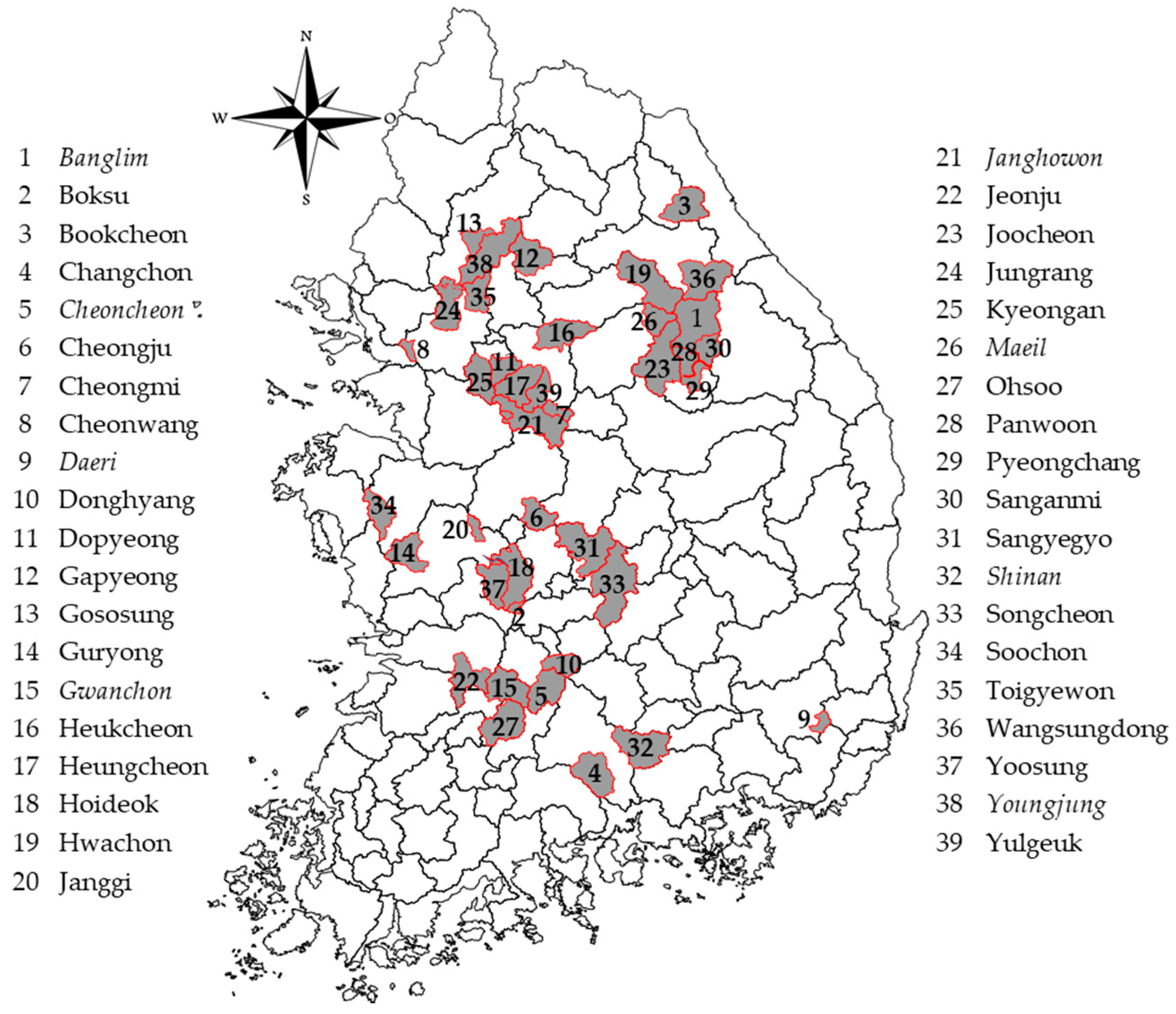
South Korea is typical of regions largely influenced by complicated geographical features. Its precipitation patterns have diverse seasonal and regional variability [38]. The elevation (area) of the watersheds included in this study vary from 26 m (42.32 km²) to 911 m (879.10 km²) above mean sea level. The average slope of the watershed ranges between 7.50% and 53.53%. The majority of the land cover (about 70.50%) is upland forests, followed by 20.26% agricultural land, urban areas (5.22%), grassland (1.56%), and other land cover distribution (2.45%). The dominant soil types are loam and sandy loam, with some fractions of silt loam. The location of watersheds is shown in Figure 1, and other details can be found in [10].

The climatic patterns over the study area are quite variable due to the Asian monsoon. Winter is extremely dry and cold, and summer is warm and moist with frequent heavy rainstorms [38]. The mean annual precipitation (from 1970 to 2000) ranged between 1000 and 1800 mm from the central to the southern regions. Approximately 50% to 60% of this precipitation falls at a high intensity and short duration from July to September [10].

2.2. Data Collection and Interpretation

Continuous rainfall and discharge data (from 2005 to 2012) for this study were collected from the Hydrological Survey Center (HSC) of South Korea. The straight-line hydrograph approach was used to separate direct runoff from the total discharge [10]. For any rain event, the prior five days’ cumulative rainfall (P₅) was used to identify the watershed antecedent moisture [10,20,22,39]. The watershed weighted curve number (CN_II) corresponding to the normal conditions were derived from the documented tables on the basis of land use/cover and soil types. The CN_I (CN_III) for dry (wet) conditions were adjusted as recommended by Mishra et al. [40].

2.3. Slope-Adjusted Curve Number Considerations and Development

Although the CN model is extensively used for predicting runoff from ungauged watersheds, one study found considerable uncertainties when tabulated CN values were applied to estimate runoff from 10 mountainous, forested watersheds in the eastern United States [9]. Similarly, another study [41] observed substantial change in the watershed CN values, ranging from 55 to 70. Moreover, the use of hydrologic soil group D (and its corresponding CN) for forested, mountainous watersheds is incompatible with the National Engineering Handbook [42] guidelines. Although very limited attention has been given to incorporate slope factors in the existing CN models [43], one study reported that adjusting handbook CN values for slope factors significantly enhanced the predicted runoff [26]. To better capture the watershed response in runoff prediction, a slope-adjusted CN is required for steep-slope, mountainous watersheds [10].

Assuming that the handbook CN value is appropriate for a 5% slope [10,17,19,20,22,23], it needs to be adjusted for steep-slope watersheds. To improve the runoff prediction capability of the CN model, the slope-adjusted CN suggested by Sharpley and Williams [17] is generally expressed as

$${\mathrm{CN}}_{\mathrm{II}\mathsf{\alpha }}={\mathrm{a}(\mathrm{CN}}_{\mathrm{III}}-{\mathrm{CN}}_{\mathrm{II}}\left)\right(1-{\mathrm{be}}^{-\mathrm{c}\times \mathsf{\alpha }}{)+\mathrm{CN}}_{\mathrm{II}}$$

(4)

where CN_IIα is the slope-adjusted CN for the antecedent runoff condition representing the watershed normal moisture (ARC-II), CN_II and CN_III are the handbook CN values obtained from watershed characteristics for ARC-II and ARC-III (wet condition), and α is the watershed average soil slope (m/m). The approach of Sharpley and Williams [17] has three empirical parameters—a, b, and c—with optimized values of 1/3, 2, and 13.86, respectively. Their adjusted relationship leads to

$${\mathrm{CN}}_{\mathrm{II}\mathsf{\alpha }}=\left(\frac{{\mathrm{CN}}_{\mathrm{III}}-{\mathrm{CN}}_{\mathrm{II}}}{3}\right)(1-{2\mathrm{e}}^{-13.86\mathsf{\alpha }}{)+\mathrm{CN}}_{\mathrm{II}}$$

(5)

Retaining the assumption of Sharpley and Williams [17] for CN_II values applicable to a 5% average slope, another study [23] developed the following relationship to adjust CN values for other slopes:

$${\mathrm{S}}_{\mathrm{II}\mathsf{\alpha }}={\mathrm{S}}_{\mathrm{II}}\left(1.1-\frac{\mathsf{\alpha }}{{\mathsf{\alpha }+\mathrm{e}}^{(3.7+0.02117\mathsf{\alpha })}}\right)$$

(6)

where S_II and S_IIα are the S values for normal moisture condition and slope-adjusted normal moisture conditions, respectively, and α is the watershed mean slope in percentage. The slope-adjusted CN can be obtained from the above equation using the general S and CN interrelationship as it is found in Equation (2). According to Huang et al. [19], the approach in Sharpley and Williams [17] has not been intensively verified in the field. Hence, they adopted a simplified approach for the CN_IIα determination on the basis of their experiments for soil slopes ranging between 0.14 and 1.40, and proposed the following relationship:

$${\mathrm{CN}}_{\mathrm{II}\mathsf{\alpha }}={\mathrm{CN}}_{\mathrm{II}}\left(\frac{322.79+15.63\mathsf{\alpha }}{\mathsf{\alpha }+323.52}\right)$$

(7)

However, this relationship is unstable because it does not follow the CN theoretical limits.

An investigation by Garg et al. [26] showed that the differences between the tabulated CN values and those calculated from the approach in Huang et al. [19] were very small when compared to that of Sharpley and Williams [17]. This is why the approach in Huang et al. [19] depicted modest improvement in estimating large as well as small runoff events and produced results very close to the original CN model with handbook CN values. Any underestimation of the runoff events using the approach in Huang et al. [19] can be attributed to the empirically selected numerical constants of Equation (7), and needs validation using the measured rainfall-runoff data.

In another study, Ajmal et al. [10] developed a slope-adjusted average CN relationship using data from 39 mountainous watersheds. They calibrated the CN_IIα using 1402 measured rainfall-runoff events from 31 watersheds and validated this with 377 rainfall–runoff events from the remaining eight watersheds. This is represented as

$${\mathrm{CN}}_{\mathrm{II}\mathsf{\alpha }}={\mathrm{CN}}_{\mathrm{II}}\left[\frac{1.9274\mathsf{\alpha }+2.13273}{\mathsf{\alpha }+2.1791}\right]$$

(8)

The above relationship was derived on the basis of data from watersheds with an average slope between 7.50% and 53.53%, where, besides other typical watershed geophysical characteristics, most of the area (approximately 70.50%) was covered with upland forests. However, their approach was also inconsistent with the CN theoretical limits on the basis of the presumption that the CN tables were originally developed with a 5% average slope in their experimental plots [10,17,19]. Knowing CN_II, CN_III, and α as the mean slope of a watershed, the proposed slope-adjusted CN (CN_IIα) in its general form is presented as

$${\mathrm{CN}}_{\mathrm{II}\mathsf{\alpha }}=\left(\frac{{\mathrm{CN}}_{\mathrm{III}}-{\mathrm{CN}}_{\mathrm{II}}}{2}\right)\left[1-{\mathrm{e}}^{-\mathrm{b}\times (\mathsf{\alpha }-0.05)}\right]{+\mathrm{CN}}_{\mathrm{II}}$$

(9)

2.4. Steps of Slope-Adjusted CN Parameter Optimization

• Data pertaining to 39 watersheds in which 1779 rainstorms events occurred provided the known values of the rainstorm events, P; the observed runoff, Q_o; and the optimized CNs for each watershed. The least squares nonlinear orthogonal distance regression objective function in Origin Pro 9.6 software produced the optimized CN values from the following equation.

  $${{\displaystyle \sum }}_{\mathrm{i}=1}^{\mathrm{n}}{\left({\mathrm{Q}}_{\mathrm{o}}-{\mathrm{Q}}_{\mathrm{e}}\right)}^2={\displaystyle \sum }{\left\{{\mathrm{Q}}_{\mathrm{o}}-\left[\frac{{\left(\mathrm{P}-0.2\times \left(\raisebox{1ex}{$25400$}\!\left/ \!\raisebox{-1ex}{$\mathrm{CN}$}\right.-254\right)\right)}^2}{\mathrm{P}+0.8\times \left(\raisebox{1ex}{$25400$}\!\left/ \!\raisebox{-1ex}{$\mathrm{CN}$}\right.-254\right)}\right]\right\}}^2=\mathrm{Minimum}$$

  (10)
• To optimize parameter b in Equation (9), the CNs obtained for the 39 watersheds from Equation (10) were divided into two sets, those of 31 watersheds (1402 rainstorm–runoff events) for calibration and those of 8 watersheds (377 rainstorm-runoff events) for validation. For calibration, the optimized CNs in step 1 were set as the target values challenging the right side of Equation (9) using the nonlinear regression least squares Levenberg–Marquardt algorithm in SPSS v.25 software. To take into account the individual watersheds’ effects on parameter b optimization, the leave-one-out (LOOV) technique was adopted. The average of 31 calibrations repetitions was the value of b = 7.125. This led to recasting the proposed CN_IIα as

  $${\mathrm{CN}}_{\mathrm{II}\mathsf{\alpha }}=\left(\frac{{\mathrm{CN}}_{\mathrm{III}}-{\mathrm{CN}}_{\mathrm{II}}}{2}\right)\left[1-{\mathrm{e}}^{-7.125\times (\mathsf{\alpha }-0.05)}\right]{+\mathrm{CN}}_{\mathrm{II}}$$

  (11)

This can also be represented as

$${\mathrm{CN}}_{\mathrm{II}\mathsf{\alpha }}=(0.5-{0.714\mathrm{e}}^{-7.125\mathsf{\alpha }}{\left)\right(\mathrm{CN}}_{\mathrm{III}}-{\mathrm{CN}}_{\mathrm{II}}{)+\mathrm{CN}}_{\mathrm{II}}$$

(12)

Introducing the CN_III conversion from CN_II after a suggestion in Mishra et al. [40] gives

$${\mathrm{CN}}_{\mathrm{III}}=\frac{{\mathrm{CN}}_{\mathrm{II}}}{0.430+{0.0057\mathrm{CN}}_{\mathrm{II}}}$$

(13)

Imputing Equation (13) into Equation (11) and simplifying it, the proposed relationship can be recast as

$${\mathrm{CN}}_{\mathrm{II}\mathsf{\alpha }}=\left[\frac{{\mathrm{CN}}_{\mathrm{II}}\left(50-{0.5\mathrm{CN}}_{\mathrm{II}}\right)}{{\mathrm{CN}}_{\mathrm{II}}+75.43}\right]\times \left[1-{\mathrm{e}}^{-7.125(\mathsf{\alpha }-0.05)}\right]{+\mathrm{CN}}_{\mathrm{II}}$$

(14)

This proposed CN_IIα relationship has twofold advantages over the previous three suggested relationships. The proposed model has only one parameter to be optimized compared to three in Sharpley and Williams [17] and Williams and Izaurralde [23], and two in Huang et al. [19], if the suggested parameter values are not applicable. Our proposed CN_IIα works within the theoretical limits (i.e., 0 to 100), unlike that in Huang et al. [19], which loses its effectiveness after CN_II = 94.27 using the highest average slope of their watersheds. Similarly, the adjustment in Williams and Izaurralde [23] and Ajmal et al. [10] also fails to follow the CN theoretical limits. The different variants of the CN model are shown in

Table 1. Models and their descriptions.

	Parameters
Model Identity	λ	CN (CNIIα)	Model Expression
M1	0.20	*NEH-4 Tables	Equations (1) and (2)
M2	0.05	NEH-4 Tables	Equations (1)–(3)
M3	0.20	Sharpley and Williams [17]	Equations (1), (2) and (5)
M4	0.20	Huang et al. [19]	Equations (1), (2) and (7)
M5	0.20	Ajmal et al. [10]	Equations (1), (2) and (8)
M6	0.20	Proposed	Equations (1), (2) and (12)
M7	0.05	Proposed	Equations (1)–(3) and (12)
M8	0.01	Proposed	Equations (1), (2) and (12)

*NEH-4: National Engineering Handbook Section-4 [42].

.

3. Statistical Analysis for Model Performance Evaluation

This study estimated the agreement between a series of observed and estimated runoffs using the root mean square error (RMSE), Nash–Sutcliffe efficiency (NSE), percent bias (PB) [34], and/or graphical assessments augmented with model performance ratings [44]. Mathematically, these indicators are

$$\mathrm{RMSE}=\sqrt{\frac{1}{\mathrm{n}}{{\displaystyle \sum }}_{\mathrm{i}=1}^{\mathrm{n}}{{(\mathrm{Q}}_{\mathrm{oi}}-{\mathrm{Q}}_{\mathrm{ei}})}^2}$$

(15)

$$\mathrm{NSE}=1-\left[\frac{{\displaystyle \sum }_{\mathrm{I}=1}^{\mathrm{n}}{{(\mathrm{Q}}_{\mathrm{oi}}-{\mathrm{Q}}_{\mathrm{ei}})}^2}{{\displaystyle \sum }_{\mathrm{I}=1}^{\mathrm{n}}{{(\mathrm{Q}}_{\mathrm{oi}}-{\overline{\mathrm{Q}}}_{\mathrm{o}})}^2}\right]$$

(16)

$$\mathrm{PB}=\left[\frac{{{\displaystyle \sum }}_{\mathrm{I}=1}^{\mathrm{n}}{(\mathrm{Q}}_{\mathrm{oi}}-{\mathrm{Q}}_{\mathrm{ei}})}{{{\displaystyle \sum }}_{\mathrm{I}=1}^{\mathrm{n}}{\mathrm{Q}}_{\mathrm{oi}}}\right]\times 100$$

(17)

where Q_oi and Q_ei are the observed and estimated runoff values for rainstorm events 1 to n, and $\overline{Q_O}$ is the mean observed runoff in each watershed. The RMSE (0 to ∞) values closer to zero depict more appropriateness of the model to estimate runoff. The NSE (−∞ to 1) illustrates how well a plot of observed vs. estimated runoff fits a 1:1 line (i.e., a perfect fit) [39]. The PB (optimum = 0) describes the average tendency of estimated values to be larger or smaller than their observed ones. Positive (negative) values indicate underestimation (overestimation) bias [44]. It is notable that perfect agreement of the estimated vs. observed data does not essentially indicate a perfect model, because observed data could have uncertainties [39]. However, we are confident about the good quality of the data used in this study. Performance evaluation of different statistical indicators and their suggested ratings [44,45] are given

Table 2. Statistical indicators and associated performance ratings [44,45].

Performance Rating	NSE [44]	NSE [45]	PB (%)
Very good	0.75 < NSE ≤ 1.00	0.90 < NSE ≤ 1.00	−10 < PB < +10
Good	0.65 < NSE ≤ 0.75	0.80 ≤ NSE ≤ 0.90	±10 ≤ PB < ±15
Satisfactory	0.50 < NSE ≤ 0.65	0.65 ≤ NSE < 0.80	±15 ≤ PB < ±25
Unsatisfactory	NSE ≤ 0.50	NSE ≤ 0.65	PB ≥ ±25

.

4. Results and Discussion

The performance evaluation of the existing models (M1–M5) and our proposed approach (M6–M8) was accomplished in two steps. First, the basic statistics of the observed runoff were compared to the models’ estimated runoff both for the calibration and validation watersheds. In the second step, commonly used statistical indicators were used to check the model’s predictive credibility [20,34,44] in conjunction with a 1:1 plot graphical judgement between the observed and modeled runoff values [46].

4.1. Models’ Analysis Based on Descriptive Statistics

The basic descriptive statistics (

Table 3. Summary statistic of rainfall (P), observed runoff (Q_o), and modeled runoff (M1–M8) in the calibration and validation watersheds.

Calibration Watersheds (1402 Rainstorm–Runoff Events)
Parameter/Model	Mean	Minimum	First Quartile (Q1)	Median	Third Quartile (Q3)	Maximum
P	80.96	12.10	39.92	59.09	98.27	519.68
Qo	38.60	0.17	8.23	19.61	49.04	348.46
M1	25.57	0.00	1.49	6.13	27.03	415.63
M2	23.56	0.00	1.14	7.26	25.79	383.27
M3	28.79	0.00	1.30	7.95	32.94	436.28
M4	26.06	0.00	1.52	6.31	28.33	419.65
M5	30.06	0.00	1.35	8.83	35.39	443.28
M6	30.26	0.00	1.23	9.38	35.34	445.73
M7	28.98	0.00	2.54	10.77	34.57	417.11
M8	39.67	0.53	7.93	20.13	49.30	458.55
Validation Watersheds (377 Rainstorm–Runoff Events)
P	75.22	20.52	40.97	57.05	86.95	376.86
Qo	35.03	0.24	8.30	19.10	43.20	364.38
M1	22.04	0.00	1.48	6.35	20.35	294.27
M2	19.85	0.00	0.85	5.55	19.93	265.59
M3	24.75	0.00	1.52	6.27	25.99	309.31
M4	22.49	0.00	1.39	6.63	21.48	296.26
M5	26.48	0.00	2.03	7.87	30.12	309.72
M6	26.07	0.00	1.71	6.66	29.04	314.48
M7	24.98	0.00	2.10	9.43	26.71	293.91
M8	34.77	0.87	7.70	17.91	40.12	325.07

Note: The highlighted values show the good agreement between the observed and the estimated runoff.

) favor the M8 model using the CN_IIα and lower λ = 0.01 followed by the M6 and M5 models. However, the M6 model was preferred over the M5 due to its practically sound CN_IIα to follow the CN theoretical bounds (0–100). In estimating runoff, the M2 model was not plausibly different from the M1 model. Therefore, lowering λ from 0.2 to 0.05, along with its corresponding CN adjustment using Equation (3), produced only modest changes in the estimated runoff values. Nonetheless, using λ = 0.05 and retaining handbook CN values without adjustment can improve the model’s runoff predictive capability, which is not shown in the assessment but is reflected in the comparison of the M6 and M7 models. The majority of the existing CN model variants underestimated the runoff in different watersheds. Nevertheless, it can be inferred that the watershed CN was not the only important parameter; selecting the proper λ also played a crucial role in estimating accurate runoff. Additionally, the prominent response of CNs to the rainstorm depth was vital in runoff depth estimation [1].

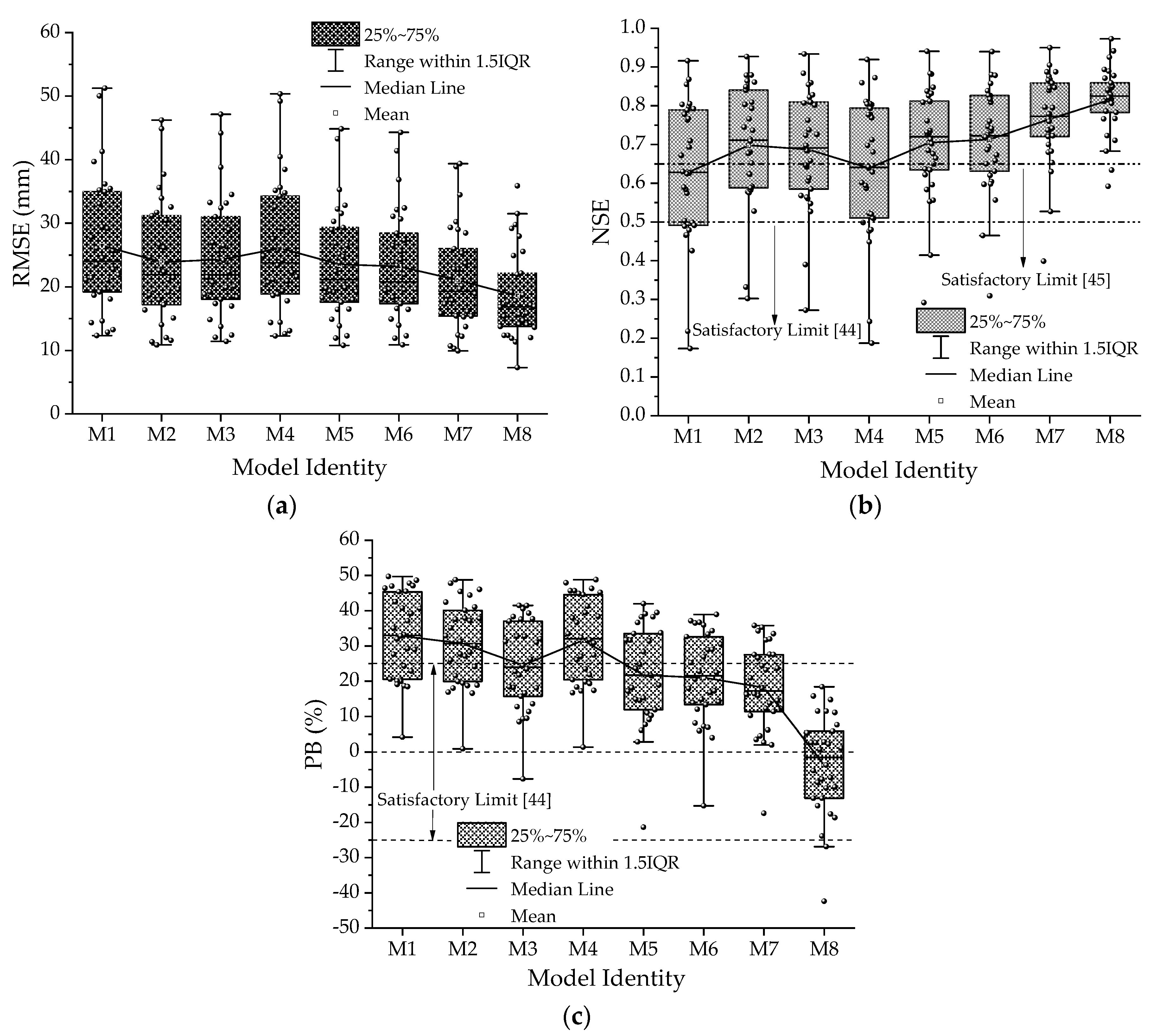
4.2. Model Performance Evaluation in Watersheds Used for Calibration

We evaluated the runoff predictability performance of the existing CN models (M1 to M5) and the proposed variants (M6 to M8) for the calibration watersheds (Figure 2). Because of minimal difference in the CN_IIα values proposed by Williams and Izaurralde [23] and Sharpley and Williams [17], we compared only the latter with the other approaches. As mentioned earlier, the RMSE can vary from 0 to ∞, and a value close to zero indicates a nearly perfect fit [15,20,34]. On the basis of the RMSE (mean, median) values, the M2 (23.90, 21.91) and M3 (24.30, 21.90) models exhibited similar but improved runoff estimation compared to the M1 (26.49, 24.02) model. The mean value for all of the statistical indicators is shown on each box plot through connected lines. The M2 model’s enhanced runoff estimation could be attributed to the lower λ = 0.05 [2], whereas the M3 model’s improved predictability could be ascribed to CN_Iiα, which was comparatively higher than the tabulated CN [17]. The M4 model (26.08, 23.78) showed almost no improvement compared to the M1 model. Comparatively better runoff prediction was found for the M5 model (23.53, 21.15), and that of the M6 model (23.23, 20.79) was almost equal in the calibration watersheds. However, the runoff predictive capabilities of the M7 model (21.06, 19.29) and M8 model (18.59, 16.87) were better, as was also evident from their overall RMSE values (Figure 2a). It can be inferred that setting a lower λ and a comparatively higher CN_Iiα, as was the case in model M8, possibly reduces the infiltration and surface water retention capacity.

Following the model performance ratings shown in Table 2 and the box plot statistics (Figure 2b), the NSE (mean, median) for the M1 model (0.58, 0.63) and the M4 model (0.59, 0.64) were the smallest among the eight variants of the CN model. It must be kept in mind that the Gusosung watershed statistics were excluded, meaning the mean and median values were calculated for the remaining 30 calibration watersheds. In that particular watershed, only the M8 model showed a reasonable runoff prediction, whereas the rest of the models’ performance indicators ratings were unsatisfactory. The M3 model (0.64, 0.68) results showed modest improvement, followed by the M2 (0.66, 0.71) and M5 (0.66, 0.71) models. However, the M6 (0.67, 0.72) and M7 (0.74, 0.77) models exhibited significantly improved results compared to the M1 model. In addition, the M8 model (0.80, 0.82) outperformed all the other models in the majority of the watersheds. The best performance of the M8 model is also evident from Figure 2b, followed by the M7 and M6 models, in that order. The lack of effectiveness of the M1 and M4 models could be attributed to the fixed and higher λ = 0.2 and inconsistent watershed tabulated CN values [10,15]. Similarly, on the basis of the PB performance ratings (Table 2), the accuracy runoff predictability of the different CN model variants is shown in Figure 2c. Using PB (mean, median), the order for accurately estimating runoff was M8 (−2.43, 0.67) > M7 (19.47, 18.06) > M6 (22.37, 22.51) > M5 (23.22, 21.93) > M3 (25.93, 24.46) > M2 (31.86, 31.26) > M4 (32.93, 32.41) > M1 (34.19, 33.14). In addition, Figure 2c shows that the PB values obtained from the M8 model in estimating runoff in the study area, except for two watersheds, were rated either very good, good, or at least satisfactory.

4.3. Models’ Performance Evaluation in Watersheds Used for Validation

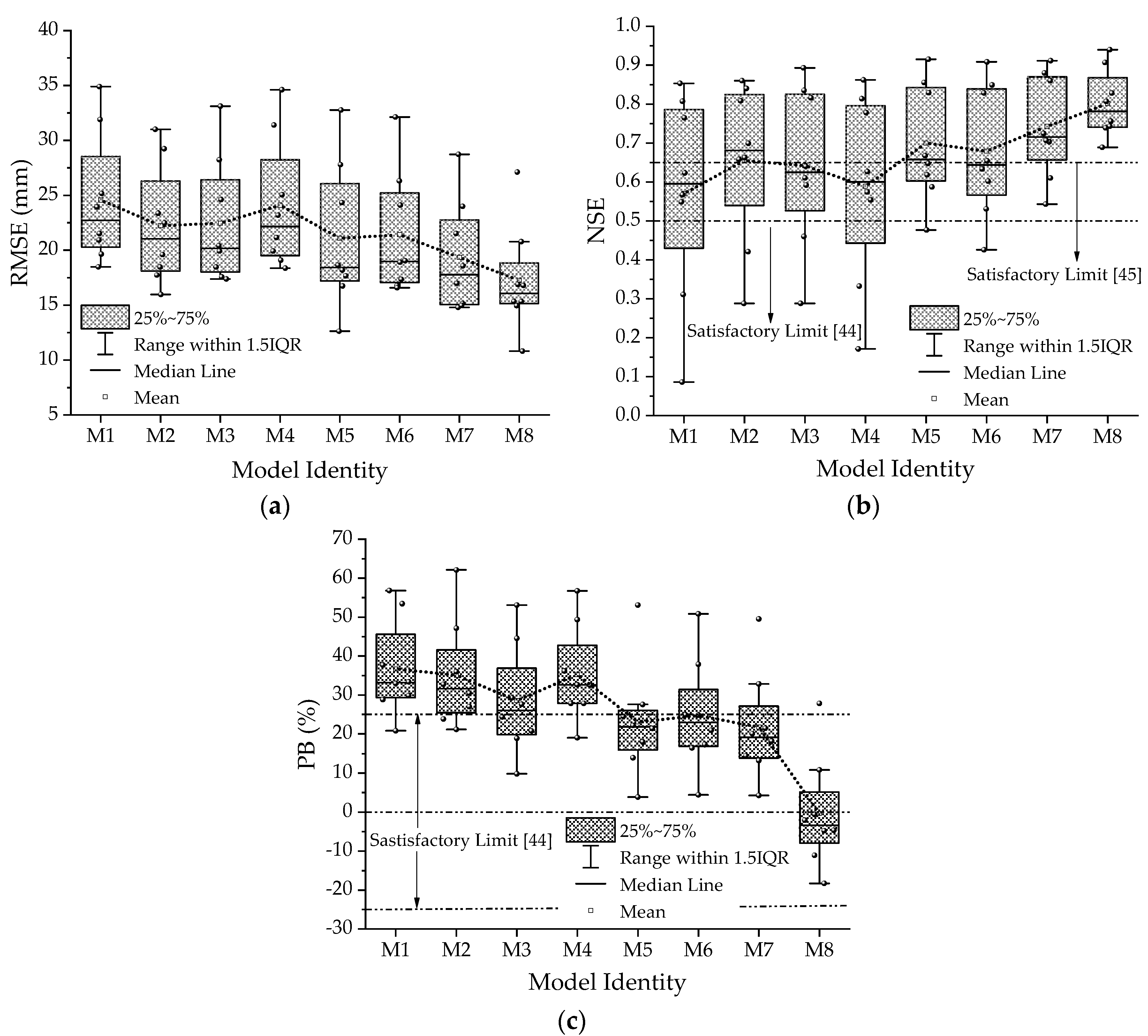
The performance of the CN model variants in the validation watersheds using the RMSE, NSE, and PB is shown in Figure 3. The superior performance of the M8 model is evident, whereas the least efficient was the M1 model with its RMSE, NSE, and PB (mean, median) values of (24.56, 22.73), (0.57, 0.60), and (36.73, 33.18), respectively. The corresponding best runoff prediction by the M8 model was recorded with RMSE (17.25, 16.07), NSE (0.80, 0.78), and PB (−0.35, −3.35). Similarly, the higher PB positive values by the M1 model in the majority of the watersheds indicated underestimation and were in the unsatisfactory range, as found by other researchers [10,20,34,44]. Nevertheless, the M8 model overestimated runoff in the majority of the watersheds, but, was within the acceptable performance range. In addition, among the remaining six variants of the CN model, the M7 model predicted more accurate runoff, followed by the M5, M6, M2, M3, and M4 models, in that order. On the basis of the PB values (Figure 3), the M8 model predicted runoff well in all the watersheds except one.

4.4. Overall Performance of Models and Comparison Based on 1:1 Plot

Table 4. Performance of the CN model and its variants in 39 watersheds in the study area.

	M1	M2	M3	M4	M5	M6	M7	M8
Performance Criteria	NSE [44]
0.75 < NSE ≤ 1.00	14	15	14	14	14	14	20	30
0.65 < NSE ≤ 0.75	3	10	7	3	10	12	13	6
0.50 < NSE ≤ 0.65	10	9	13	13	11	9	4	2
NSE ≤ 0.50	12	5	5	9	4	4	2	1
	NSE [45]
0.90 < NSE ≤ 1.00	1	1	1	1	2	2	3	5
0.80 ≤ NSE ≤ 0.90	6	12	12	8	11	11	11	20
0.65 ≤ NSE < 0.80	10	12	8	8	11	13	19	11
NSE ≤ 0.65	22	14	18	22	15	13	6	3
	PB (%)
−10 < PB < +10	1	1	5	1	5	6	6	19
±10 ≤ PB < ±15	0	0	3	0	6	5	8	9
±15 ≤ PB < ±25	10	11	12	10	13	12	12	7
PB ≥ ±25	28	27	19	28	15	16	13	4

summarizes the credibility of the eight variants of the CN model in estimating runoff from rainstorm events in different watersheds. It is obvious that the M8 model exhibited more accurate results for a very good performance rating based on NSE (PB) in 30 (19) out of 39 watersheds. The corresponding goodness-of-fit ratting for the M1 model was found only in 14 (1) watershed(s). Applying the model evaluation criteria recommended by Ritter and Muñoz-Carpena [45], the M1 and M4 model predictions were “satisfactorily” to “very good” in only 43.6% of the watersheds, followed by the M3, M5, M2, M6, and M7 models with their corresponding values of 53.9%, 61.5%, 64.1%, 66.7%, and 84.6% of the watersheds, respectively. The more plausible model for efficiently predicting runoff was M8 in 92.3% (36 out of 39) watersheds. It is notable that the majority of the runoff was underestimated by the M1 model, as has also been reported for rangeland and cropland in Montana and Wyoming [47], Mississippi [48], the Loess Plateau of China [19], India [20,22,26,43], South Korea [10,15], and Poland [49]. After M8, the M7 and M6 models predicted runoff more coincident with the observed values. The M4 model’s inferior performance could possibly be linked to very little difference in the CN_IIα and the handbook CN values (CN_IIα–CN), which varied in the range of 0.73 to 1.46. The corresponding CN differences for the M3, M5, and M6 models were in the range of 1.37 to 6.52, 0.73 to 11.28, and 1.15 to 9.48, respectively. It is notable that the M6 and M8 models used the same CN_IIα values. The M8 model’s outperformance in predicting runoff was probably because of its lower λ = 0.01, as suggested for Korean steep-slope watersheds [10], and its comparatively higher CN_IIα values.

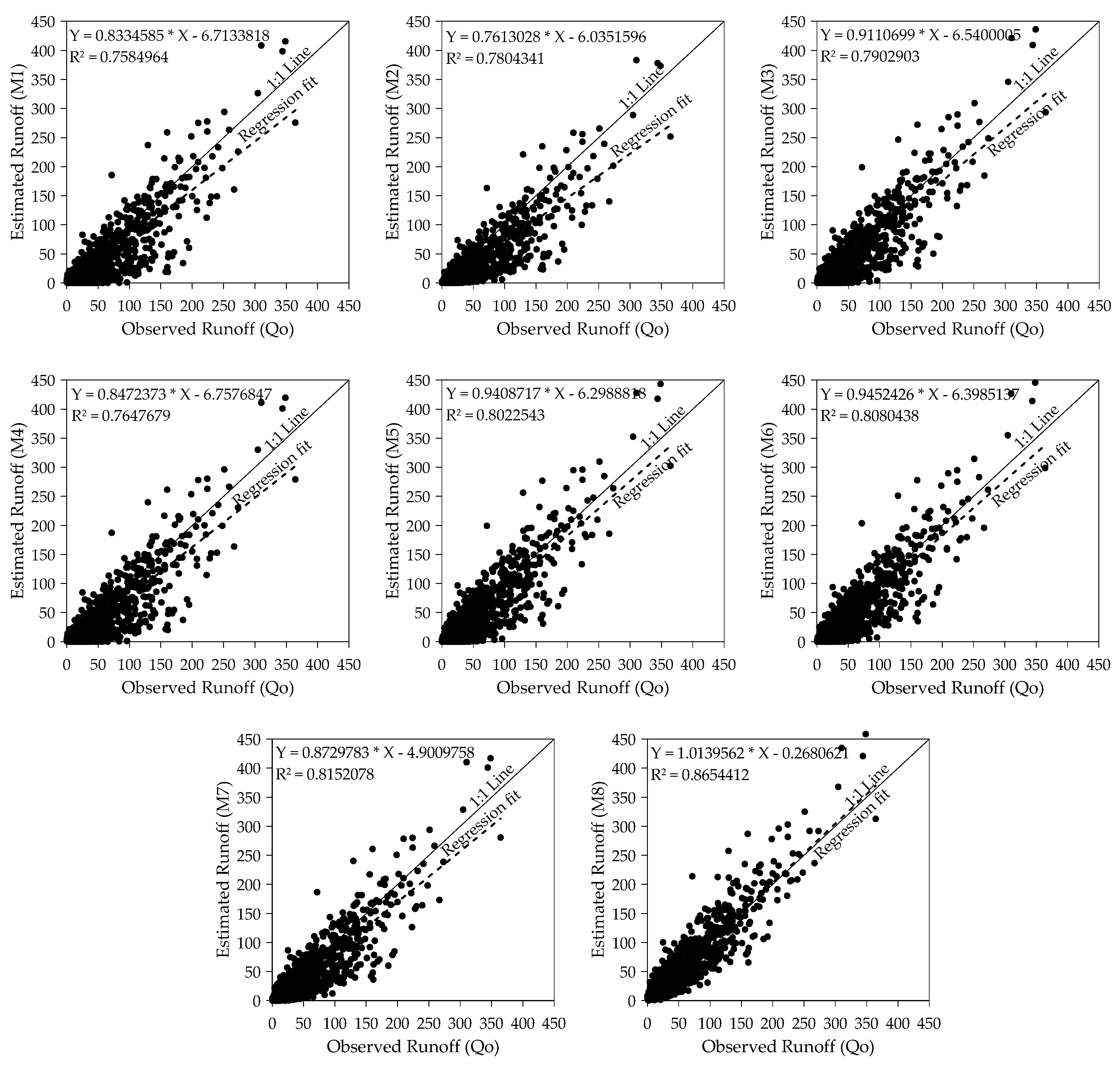
We further compared the different CN model variants on the basis of cumulative observed and estimated runoff from the 39 watersheds using the 1:1 plot and the coefficient of determination, R². The moderately high R² value supported better runoff prediction capability of the M2 model compared to the M1 model. However, deviation of the observed–estimated runoff best-fit-regression line from the 1:1 plot shows that both the M1 and M2 models underestimated the majority of the runoff events (Figure 4). Although the M2 model R² value was comparatively high, the runoff predictability of the M1, M2, and M4 models was almost indistinguishable. Nevertheless, the closeness of data points around the 1:1 plot and the higher R² values of the M5 through M8 models favored these models for comparatively better runoff prediction. The best agreement between the observed and estimated runoff was evidenced by applying the M8 model, as shown in Figure 4. It should be noted that the R² statistics used for model evaluation could mislead practitioners. These statistics are oversensitive to extremely high values and insensitive to additive and proportional differences between model predictions and measured data [44]. The overall promising results of the M8 model support its suitability for runoff prediction in the steep-slope watersheds. Therefore, the original CN model and the majority of its variants discussed here do not well represent complex watershed characteristics, and thus the abstraction coefficient, the CN values from watershed, and the CN model itself need to be revised for general application. A very recent and comprehensive review by the NRCS Task Group on Curve Number Hydrology [5] also suggested changes to update the handbook and its associated procedures on the basis of lessons learned from global experiences and additional data analyses. To avoid jumps in runoff estimation, the CN model could be made to be more robust by not fixing the initial abstraction coefficient and considering the effect of rainfall as well as the spatial and temporal variability while estimating the watershed CN values.

There is an evidence that the CN tables that were documented a few decades back that were based on soils and land use/cover are often wide of the mark and not supported by real ground data or by critical analyses [10,15,50]. The original CN model response demonstrated in different studies is very sensitive in selecting the watershed-representative CN. Moreover, the runoff response from some watersheds were found to be very erratic, leading to great discrepancies between the modeled data and reality [50]. Like our findings, various studies have reported underestimated runoff in the steep-slope watersheds using the original CN methodology [10,17,18,19,20,21,22,23], and slope adjustment for CN was proposed to capture the watershed response in predicting runoff [10,17,18,19,21,22,23,24]. Application of the suggested approach by Sharpley and Williams [17] was criticized for being tested with very limited data in the field [19]. To support the findings of Williams et al. [18], two other slope-adjusted CN approaches were developed by Ajmal et al. [10] and Sharpley and Williams [17], but they were not structurally sound due to incapability to follow the CN theoretical limits. Because of the plausible response in replicating the watershed runoff, the slope-adjusted CN approach proposed in this study was not only structurally sound in terms of following the theoretical bounds of the CN, but also in supporting its application for better runoff prediction. However, the model results could be further improved by introducing the effects of spatial variability in CN for the soil–cover complex along watersheds [51,52].

5. Conclusions and Practical Implications

The CN model is being updated continuously on the basis of new measured rainfall–runoff data and innovation in research. When handbook CN values are used, the inconsistent runoff prediction capability of this model has led researchers to adjust the CN values using the effect of rainfall magnitudes [2,5] and watershed slope [10,17,18,19,24,26]. However, some researchers agree that the handbook CN values are fit for runoff estimation from watersheds with a maximum 5% average slope. Hence, there is a room for further refinement in determining CN values. This study investigated and proposed a practically sound slope-adjusted CN (CN_IIα) approach to improve the runoff prediction capability of the CN model in steep-slope watersheds in order to reduce possible uncertainties. The proposed CN_IIα not only followed the theoretical limits (0, 100) [17], but in addition, unlike other existing CN_IIα approaches [10,19,23], it provided a promising runoff prediction capability in the study area. The use of λ = 0.05 in place of λ = 0.2 and their adjusted CN_0.05 values modestly improved the CN model runoff predictability, but not well enough for runoff estimation from steep-slope watersheds. On the basis of different performance indicators, we found that the proposed CN_IIα had a positive impact on the CN model runoff prediction. Users of the CN model should know the limitations in its procedures and assumptions because the model produces diverse responses when applied to different land types and watersheds [5]. Assuming a fixed λ value and its associated three fixed values of initial abstraction for dry, normal, and wet conditions are among the major limitations of the original CN model and variants used in this study. The model needs an overhaul for various compelling reasons to circumvent the fixed λ value, as well as unjustified sudden jumps in CN values and its associated estimated runoff. In this era of cutting-edge technology, researchers of different biomes have introduced new parameters in the model to improve its runoff prediction capability. However, inculcating new parameters has increased the model complexity and restricted its application in ungauged watersheds. The CN methodology must be overhauled using experiences from the modern hydrologic engineering without losing the simplicity rule.

References

- Muche, M.E.; Hutchinson, S.L.; Hutchinson, J.S.; Johnston, J.M. Phenology-adjusted dynamic curve number for improved hydrologic modeling. J. Environ. Manag. 2019, 235, 403–413. [Google Scholar] [CrossRef] [PubMed]
- Hawkins, R.H.; Ward, T.J.; Woodward, D.E.; Van Mullem, J.A. ASCE EWRI Task Committee Report on State of the Practice in Curve Number Hydrology; ASCE: Reston, VA, USA, 2009; Volume 106. [Google Scholar]
- Fan, F.; Deng, Y.; Hu, X.; Weng, Q. Estimating composite curve number using an improved SCS-CN method with remotely sensed variables in Guangzhou, China. Remote Sens. 2013, 5, 1425–1438. [Google Scholar] [CrossRef] [Green Version]
- Beck, H.E.; van Dijk, A.I.; de Roo, A.; Dutra, E.; Fink, G.; Orth, R.; Schellekens, J. Global evaluation of runoff from ten state-of-the-art hydrological models. Hydrol. Earth Sys. Sci. 2017, 21, 2881–2903. [Google Scholar] [CrossRef] [Green Version]
- Hawkins, R.H.; Theurer, F.D.; Rezaeianzadeh, M. Understanding the basis of the curve number method for watershed models and TMDLs. J. Hydrol. Eng. 2019, 24, 06019003. [Google Scholar] [CrossRef]
- Ling, L.; Yusop, Z.; Chow, M.F. Urban flood depth estimate with a new calibrated curve number runoff prediction model. IEEE Access 2020, 8, 10915–10923. [Google Scholar] [CrossRef]
- Pandit, A.; Heck, H.H. Estimations of soil conservation service curve numbers for concrete and asphalt. J. Hydrol. Eng. 2009, 14, 335–345. [Google Scholar] [CrossRef]
- Stewart, D.; Canfield, E.; Hawkins, R. Curve number determination methods and uncertainty in hydrologic soil groups from semiarid watershed data. J. Hydrol. Eng. 2012, 17, 1180–1187. [Google Scholar] [CrossRef]
- Tedela, N.H.; McCutcheon, S.C.; Rasmussen, T.C.; Hawkins, R.H.; Swank, W.T.; Campbell, J.L.; Adams, M.B.; Jackson, C.R.; Tollner, E.W. Runoff curve numbers for 10 small forested watersheds in the mountains of the eastern United States. J. Hydrol. Eng. 2012, 17, 1188–1198. [Google Scholar] [CrossRef] [Green Version]
- Ajmal, M.; Waseem, M.; Ahn, J.-H.; Kim, T.-W. Runoff estimation using the NRCS slope-adjusted curve number in mountainous watersheds. J. Irrig. Drain. Eng. 2016, 142, 04016002. [Google Scholar] [CrossRef]
- Fu, S.; Zhang, G.; Wang, N.; Luo, L. Initial abstraction ratio in the SCS-CN method in the Loess Plateau of China. Trans. ASABE 2011, 54, 163–169. [Google Scholar] [CrossRef]
- D’Asaro, F.; Grillone, G. Empirical investigation of curve number method parameters in the Mediterranean area. J. Hydrol. Eng. 2012, 17, 1141–1152. [Google Scholar] [CrossRef]
- D’Asaro, F.; Grillone, G.; Hawkins, R.H. Curve number: Empirical evaluation and comparison with curve number handbook tables in Sicily. J. Hydrol. Eng. 2014, 19, 04014035. [Google Scholar] [CrossRef]
- Singh, P.K.; Mishra, S.K.; Berndtsson, R.; Jain, M.K.; Pandey, R.P. Development of a modified SMA based MSCS-CN model for runoff estimation. Water Res. Manag. 2015, 29, 4111–4127. [Google Scholar] [CrossRef]
- Ajmal, M.; Kim, T.-W. Quantifying excess stormwater using SCS-CN–based rainfall runoff models and different curve number determination methods. J. Irrig. Drain. Eng. 2015, 141, 04014058. [Google Scholar] [CrossRef]
- Baltas, E.; Dervos, N.; Mimikou, M. Determination of the SCS initial abstraction ratio in an experimental watershed in Greece. Hydrol. Earth Sys. Sci. 2007, 11, 1825–1829. [Google Scholar] [CrossRef] [Green Version]
- Sharpley, A.; Williams, J. Epic—Erosion/Productivity Impact Calculator: I. Model Documentation. II: User Manual; Technical Bulletin, No. 1768 1990; United State Department of Agriculture: Washington, DC, USA, 1990.
- Williams, J.R.; Izaurralde, R.C.; Steglich, E.M. Agricultural policy/environmental extender model. Theor. Doc. Version 2008, 604, 2008–2017. [Google Scholar]
- Huang, M.; Gallichand, J.; Wang, Z.; Goulet, M. A modification to the soil conservation service curve number method for steep slopes in the Loess Plateau of China. Hydrol. Process. 2006, 20, 579–589. [Google Scholar] [CrossRef]
- Deshmukh, D.S.; Chaube, U.C.; Hailu, A.E.; Gudeta, D.A.; Kassa, M.T. Estimation and comparision of curve numbers based on dynamic land use land cover change, observed rainfall-runoff data and land slope. J. Hydrol. 2013, 492, 89–101. [Google Scholar] [CrossRef]
- Ebrahimian, M.; Nuruddin, A.A.B.; Soom, M.A.B.M.; Sood, A.M.; Neng, L.J. Runoff estimation in steep slope watershed with standard and slope-adjusted curve number methods. Pol. J. Environ. Stud. 2012, 21, 1191–1202. [Google Scholar]
- Mishra, S.K.; Chaudhary, A.; Shrestha, R.K.; Pandey, A.; Lal, M. Experimental verification of the effect of slope and land use on scs runoff curve number. Water Res. Manag. 2014, 28, 3407–3416. [Google Scholar] [CrossRef]
- Williams, J.; Izaurralde, R. The APEX model. In Watershed Models; CRC Press: Boca Raton, FL, USA, 2005. [Google Scholar]
- Williams, J.; Kannan, N.; Wang, X.; Santhi, C.; Arnold, J. Evolution of the SCS runoff curve number method and its application to continuous runoff simulation. J. Hydrol. Eng. 2012, 17, 1221–1229. [Google Scholar] [CrossRef]
- Fang, H.; Cai, Q.; Chen, H.; Li, Q. Effect of rainfall regime and slope on runoff in a gullied loess region on the Loess Plateau in China. Environ. Manag. 2008, 42, 402–411. [Google Scholar] [CrossRef] [PubMed]
- Garg, V.; Nikam, B.R.; Thakur, P.K.; Aggarwal, S. Assessment of the effect of slope on runoff potential of a watershed using NRCS-CN method. Int. J. Hydrol. Sci. 2013, 3, 141–159. [Google Scholar] [CrossRef]
- Slattery, M.C.; Bryan, R.B. Hydraulic conditions for rill incision under simulated rainfall: A laboratory experiment. Earth Surf. Process. Landf. 1992, 17, 127–146. [Google Scholar] [CrossRef]
- Govers, G. A field study on topographical and topsoil effects on runoff generation. Catena 1991, 18, 91–111. [Google Scholar] [CrossRef]
- Fox, D.; Bryan, R.; Price, A. The influence of slope angle on final infiltration rate for interrill conditions. Geoderma 1997, 80, 181–194. [Google Scholar] [CrossRef]
- Van de Giesen, N.; Stomph, T.J.; de Ridder, N. Surface runoff scale effects in west African watersheds: Modeling and management options. Agric. Water Manag. 2005, 72, 109–130. [Google Scholar] [CrossRef]
- Joel, A.; Messing, I.; Seguel, O.; Casanova, M. Measurement of surface water runoff from plots of two different sizes. Hydrol. Process. 2002, 16, 1467–1478. [Google Scholar] [CrossRef]
- Stomph, T.; De Ridder, N.; Steenhuis, T.; Van de Giesen, N. Scale effects of hortonian overland flow and rainfall-runoff dynamics: Laboratory validation of a process-based model. Earth Surf. Process. Landf. 2002, 27, 847–855. [Google Scholar] [CrossRef]
- Esteves, M.; Lapetite, J.M. A multi-scale approach of runoff generation in a sahelian gully catchment: A case study in Niger. Catena 2003, 50, 255–271. [Google Scholar] [CrossRef]
- Lal, M.; Mishra, S.; Pandey, A.; Pandey, R.; Meena, P.; Chaudhary, A.; Jha, R.K.; Shreevastava, A.K.; Kumar, Y. Evaluation of the soil conservation service curve number methodology using data from agricultural plots. Hydrogeol. J. 2017, 25, 151–167. [Google Scholar] [CrossRef]
- Mah, M.; Douglas, L.; Ringrose-Voase, A. Effects of crust development and surface slope on erosion by rainfall. Soil Sci. 1992, 154, 37–43. [Google Scholar] [CrossRef]
- Kowalik, T.; Walega, A. Estimation of CN parameter for small agricultural watersheds using asymptotic functions. Water 2015, 7, 939–955. [Google Scholar] [CrossRef] [Green Version]
- Lian, H.; Yen, H.; Huang, C.; Feng, Q.; Qin, L.; Bashir, M.A.; Wu, S.; Zhu, A.-X.; Luo, J.; Di, H. CN-China: Revised runoff curve number by using rainfall-runoff events data in China. Water Res. 2020, 177, 115767. [Google Scholar] [CrossRef] [PubMed]
- Qiu, L.; Im, E.-S.; Hur, J.; Shim, K.-M. Added value of very high resolution climate simulations over South Korea using WRF modeling system. Clim. Dyn. 2019, 54, 173–189. [Google Scholar] [CrossRef]
- Isik, S.; Kalin, L.; Schoonover, J.E.; Srivastava, P.; Lockaby, B.G. Modeling effects of changing land use/cover on daily streamflow: An artificial neural network and curve number based hybrid approach. J. Hydrol. 2013, 485, 103–112. [Google Scholar] [CrossRef]
- Mishra, S.K.; Jain, M.K.; Suresh Babu, P.; Venugopal, K.; Kaliappan, S. Comparison of AMC-dependent CN-conversion formulae. Water Res. Manag. 2008, 22, 1409–1420. [Google Scholar] [CrossRef]
- McCutcheon, S.; Tedela, N.; Adams, M.; Swank, W.; Campbell, J.; Hawkins, R.; Dye, C. Rainfall-Runoff Relationships for Selected Eastern us Forested Mountain Watersheds: Testing of the Curve Number Method for Flood Analysis; West Virginia Division of Forestry: Charleston, WV, USA, 2006. [Google Scholar]
- NRCS (Natural Resources Conservation Service). National Engineering Handbook Section-4, Part 630, Hydrology; NRCS: Washington, DC, USA, 2001.
- Lal, M.; Mishra, S.K.; Pandey, A. Physical verification of the effect of land features and antecedent moisture on runoff curve number. Catena 2015, 133, 318–327. [Google Scholar] [CrossRef]
- Moriasi, D.N.; Arnold, J.G.; Van Liew, M.W.; Bingner, R.L.; Harmel, R.D.; Veith, T.L. Model evaluation guidelines for systematic quantification of accuracy in watershed simulations. Trans. ASABE 2007, 50, 885–900. [Google Scholar] [CrossRef]
- Ritter, A.; Muñoz-Carpena, R. Performance evaluation of hydrological models: Statistical significance for reducing subjectivity in goodness-of-fit assessments. J. Hydrol. 2013, 480, 33–45. [Google Scholar] [CrossRef]
- Harmel, R.; Smith, P.; Migliaccio, K.; Chaubey, I.; Douglas-Mankin, K.; Benham, B.; Shukla, S.; Muñoz-Carpena, R.; Robson, B.J. Evaluating, interpreting, and communicating performance of hydrologic/water quality models considering intended use: A review and recommendations. Environ. Model. Softw. 2014, 57, 40–51. [Google Scholar] [CrossRef]
- Van Mullem, J. Runoff and peak discharges using Green-Ampt infiltration model. J. Hydraul. Eng. 1991, 117, 354–370. [Google Scholar] [CrossRef]
- King, K.W.; Arnold, J.; Bingner, R. Comparison of Green-Ampt and curve number methods on Goodwin Creek watershed using SWAT. Trans. ASAE 1999, 42, 919. [Google Scholar] [CrossRef]
- Walega, A.; Salata, T. Influence of land cover data sources on estimation of direct runoff according to SCS-CN and modified SME methods. Catena 2019, 172, 232–242. [Google Scholar] [CrossRef]
- Hawkins Richard, H. Curve Number Method: Time to Think Anew? J. Hydrol. Eng. 2014, 19, 1059. [Google Scholar] [CrossRef]
- Soulis, K.X.; Valiantzas, J.D. Identification of the SCS-CN parameter spatial distribution using rainfall-runoff data in heterogeneous watersheds. Water Res. Manag. 2013, 27, 1737–1749. [Google Scholar] [CrossRef]
- Soulis, K.X. Estimation of SCS curve number variation following forest fires. Hydrol. Sci. J. 2018, 63, 1332–1346. [Google Scholar] [CrossRef]
Figure 1.
Location of watersheds in the study area. The watersheds in italics were used for validation.
Figure 2.
(a) Root mean square error (RMSE), (b) Nash–Sutcliffe efficiency (NSE), and (c) percent bias (PB) for eight variants of the CN model using data of 30 out of 31 calibration watersheds.
Figure 3.
(a) RMSE, (b) NSE, and (c) PB for eight variants of the CN model using data of eight validation watersheds.
Figure 4.
Observed and estimated runoff comparison for eight variants of the CN model using cumulative data of all 39 watersheds.