Heavy Precipitation Systems in Calabria Region (Southern Italy): High-Resolution Observed Rainfall and Large-Scale Atmospheric Pattern Analysis

Abstract

An in-depth analysis of historical heavy rainfall fields clearly constitutes an important aspect in many related topics: as examples, mesoscale models for early warning systems and the definition of design event scenarios can be improved, with the consequent upgrading in the prediction of induced phenomena (mainly floods and landslides) into specific areas of interest. With this goal, in this work the authors focused on Calabria region (southern Italy) and classified the main precipitation systems through the analysis of selected heavy rainfall events from high resolution rain gauge network time series. Moreover, the authors investigated the relationships among the selected events and the main synoptic atmospheric patterns derived by the European Centre for Medium-Range Weather Forecasts (ECMWF) ERA5 Reanalysis dataset, in order to assess the possible large-scale scenarios which can induce heavy rainfall events in the study area. The obtained results highlighted: (i) the importance of areal reduction factors, rainfall intensities and amounts in order to discriminate the investigated precipitations systems for the study area; (ii) the crucial role played by the position of the averaged low-pressure areas over the Mediterranean for the synoptic systems, and by low-level temperature for the convective systems.

1. Introduction

The classification of the main atmospheric patterns related to heavy rainfall fields plays an important role in many topics concerning rainfall modelling and forecasting; moreover, it is very useful for the definition of event scenarios and subsequent risk evaluation for a prefixed study area.

As reported in [1], precipitation systems can be mainly regrouped in convective and stratiform events, and the main worldwide observed rainfall patterns can be considered as a combination of these two components. Focusing on the Mediterranean area, the weather systems are usually grouped into three main classes [2,3,4]: synoptic systems, which are the prevalent ones; convective systems, mainly associated to heat-related instability and Tropical-Like Cyclones (TLC), or Medicanes, which are very intense but less frequent with respect to the previous ones.

The first group comprises rainfall events with an extension of about 10³–10⁴ km² [5], in which cells, or clusters of cells, with a high intensity are often visible. The duration for these events usually varies from several hours to several days. Moreover, their motion regards hundreds of kilometers (according to the atmospheric circulation) and ordinary extreme events (i.e., more frequent and less severe on average) are associated. The maximum values for rainfall intensity usually range from 40 to 140 mm/day [6].

The second group usually regards isolated storm cells, which have a spatial extent of about 10–50 km² [7], or clusters of these. They are associated with convective movements of warm moist air masses towards the cold layers of the overlying atmosphere. They could be also supported by contributions of energy and water vapor from limited areas, carried by a convergent flow of air masses. The instantaneous and average rainfall intensities can vary in a wide range, typically 10–100 mm/h; the total duration could be from one to several hours, depending on the number of active cells to be dissipated.

Lastly, vortices of great intensity and small scale are mainly associated with the third group [8], generally occurring between August and November. TLCs are usually characterized by strong winds (up to 180 km/h), and a duration from a minimum of 6 h to a maximum of five days. The most frequent genesis occurs on the Ionian Sea and the Balearic Sea, with a sea surface temperature (SST) of at least 15 °C; this threshold is less than that for tropical cyclones [9,10,11,12]. The resulting rainfall intensities are much higher when compared with the phenomena related to the first group (i.e., synoptic systems). These events usually generate cumulative rainfall up to 30%–50% of Mean Annual Precipitation (MAP), covering areas up to 100–1000 km² in less than 24 h.

In this context, an important role is played by the study of the main large-scale atmospheric patterns related to the heavy precipitation events, which can be particularly useful for analysis and modelling of Extraordinary Extreme Events (EEEs). EEEs are also indicated as “outliers” or “superextremes” (i.e., events with very high return periods), and they constitute a topic with an increasing interest for the scientific community, as reported in [13,14,15].

In the Mediterranean, [16] performed an atmospheric pattern classification starting by nine years of rain data and using model outputs at 0.5° spatial resolution. Similar approach was used by [17] (7.5 years were analyzed with 0.5° resolution model outputs) and [18] (10 years were analyzed using European Centre for Medium-Range Weather Forecasts (ECMWF) gridded analysis at 0.75° resolution).

This paper focuses on Calabria region (southern Italy), located in the central part of the Mediterranean area. The region is particularly prone to heavy rain events. Many of these events were examined in several papers, both in terms of statistical/climatological analysis [19,20,21] and for the reconstruction of singular extreme occurrences [22,23], in order to understand their characteristics and dynamic. The study of [20] presented the first exploratory results and analyses performed on a 30-year (1978–2007) homogeneous precipitation database for the Calabria region; the authors considered complete time series of daily precipitations from 88 rain gauges over the region. It followed that the orography and the sea have a major role, while the seasonal dependence of rainfall unequivocally reveals the influence of the synoptic scale conditions. Above all, despite the fact that yearly precipitation is larger on the west side of the peninsula, most intense rainstorms affect mainly the east side, where these heavy storms are more frequent. [24] provided an atmospheric patterns classification for Calabria region: the authors selected and regrouped 92 heavy rainfall events in an eight-year period, by analyzing rain gauge daily data and outputs of the mesoscale meteorological model Regional Atmospheric Modeling System (RAMS) [25,26].

This work represents an extension of the above-cited studies, with a twofold observational and modeling approach; in fact:

• a deeper statistical analysis of the rain gauge data, at a finer temporal resolution, is performed, and a larger period of investigation is considered (14 years);
• with the proposed modeling approach, the meteorological conditions that influence the heavy rain events and their spatiotemporal behavior are analyzed. Obviously, this study should not be considered as an alternative to Numerical Weather Prediction models. It represents a survey that can provide very useful information in the more general topic regarding analysis of rainfall fields, mainly in order to evaluate the role of the considered synoptic parameters as possible precursors. In particular, noticeable improvements can be obtained in the definition of design rainfall scenarios in space and time, with consequent progress for evaluation of risk scenarios related to induced phenomena (mainly floods and landslides).

The paper is organized in two main parts:

• in the first part, the authors selected and regrouped heavy events by using sub-hourly data series from a rain gauge network;
• in the second part, the authors investigated the relationships among the selected events and the main synoptic atmospheric patterns derived by the Reanalysis (ERA5) dataset of the European Centre for Medium-Range Weather Forecasts (ECMWF), in order to assess the possible large-scale scenarios which can induce heavy rainfall events in the study area.

2. Materials and Methods

2.1. Study Area

Calabria region (southern Italy) is located in the central part of the Mediterranean area and it presents peculiar micro-climatic characteristics; the meteorological phenomena are strongly related to its geographic position as well as to the its geomorphological features. The western coast of the region is bordered by the Tyrrhenian Sea, while the east and south coasts by the Ionian Sea. The total area is about 15,000 km²; it is hilly for 49.2% and mountainous for 41.8% of the territory, respectively. The main mountains, which reach altitudes up to 2000 m, are: Pollino, Catena Costiera, Sila, Serre, Aspromonte.

In regards to precipitation fields, a study carried out by [21] for the period 1970–2006 indicated higher values of Mean Annual Precipitation (MAP) in mountain areas, such as Pollino (1400 mm), Sila (1200 mm), Serre (1500 mm) and Aspromonte (1400 mm), while lower values occur on the coastal areas east of Pollino (600 mm) and east of Sila (700 mm). This difference is due to the “barrier effect” made by the mountains when the perturbations usually hit Calabria from west to east. Indeed, as explained by [20], most rainfall events are due to cyclones that develop close to the Alps and in the western part of the Mediterranean, which impact on the Tyrrhenian side, moving from west to east. Cyclones from North Africa and the Balkans are less frequent and mainly affect the Ionian side. In general, in the western part of Calabria there are the greatest rain amounts, while in the eastern part the most extreme events occur, as they are exposed to more intense cyclones [24].

2.2. Selection and Classification of Rain Events

The authors used the 20-min data series until 2015, downloaded from the website of the Multi Risk Functional Center of Calabria region (www.cfd.calabria.it). The whole network consists of 155 rain gauges (Figure 1) and the density is about 1 rain gauge in 100 km².

The use of high ∆t-resolution rainfall series is justified by the fact that precipitation is characterized by a high spatial-temporal variability [27] (especially in the Mediterranean area), and therefore sub-hourly information is useful in detailing many events features as much as possible.

In order to work with a consistent rain gauge database, only the data from 2002 to 2015 were taken into consideration, in which at least 100 stations recorded data at the same time. The goal was to have a density of at least one working rain gauge in 150 km².

The selection of heavy rainfall events in space and time was carried out by using a threshold criterion. In this work, starting from 20-min rainfall time series, it was assumed that a heavy event occurs when the rain intensity observed in at least one rain gauge exceeds 16 mm/20 min (i.e., 48 mm/h, see [28]), indicated as I_EVE. Specifically, an event:

• starts when a value higher than I_MIN = 5 mm/20 min (minimum threshold) is observed in at least one rain gauge (located in the spatial domain), and no station records a value greater than or equal to the aforementioned threshold I_MIN in the previous 6 h;
• ends when all the rain gauges in the spatial domain measure values that are lower than I_MIN after the rain peak (which has to be greater than or equal to I_EVE), and no station recorded values higher than I_MIN in the following 6 h.

The waiting time between two consecutive rainfall events was assumed to be at least 6 h, as defined in [29].

For each selected rainfall event, the authors identified:

• the duration d (h);
• the maximum observed value of rainfall amount (mm) in 20 min, from rain gauge network;
• the maximum observed values of cumulative rainfall amount (mm) from rain gauge network, aggregated along the whole event duration and on specific durations (1, 3, 6, 12 and 24 h);
• the associated map of the rainfall field, which was obtained by using the Inverse Distance Weighting (IDW) method [30] for a 1-km resolution grid, and by considering the cumulative rainfall amounts, over the whole event duration, from rain gauge data. IDW is one of the most used deterministic interpolation methods to reproduce rainfall fields. Several studies compared different interpolation techniques concerning rainfall data, and asserted that IDW method is comparable or even more suitable than other techniques (including geostatistics approaches) for finer temporal resolutions, such as a daily resolution or less [31,32,33,34,35,36]. Moreover, having to perform a large number of interpolations, the use of IDW requires shorter computation times than others [33,37];
• from the obtained rainfall field, the maximum value of cumulative rainfall amount (mm) was calculated; it was aggregated on several spatial and time resolutions. The authors considered nxn pixel—moving square grids, with n = 1, 5, 11, 21, 45 and 51 km, and durations equal to 1, 3, 6, 12 and 24 h.

Then, the final step for this part was the regrouping in classes. In technical literature, many methodologies are suggested; the most applied for circulation pattern classification are the Principal Component Analysis (PCA) [38,39] and Cluster Analysis (CA) [40,41]. Scientific discussion on these methods and their climatic applications is extensive [38,40,42,43,44,45].

In this work, the authors proposed a heuristic procedure for regrouping the selected events. This is characterized by an in-depth analysis of each event, firstly in terms of visual inspection of the map related to the aggregated rainfall field over the whole specific duration, and then by analysing the values assumed by maximum intensities (point and areal), duration, and spatial extension. This investigation, although time consuming, can clearly be very useful, because it allows to better understand the specific dynamics in space and time of each event, from which it could be more suitable the selection of the main discriminant aspects from a class to another.

Concerning visual inspection, it is expected that convective events are characterized by intense and localized peaks which are spatially separated by areas without precipitation [46,47,48], while synoptic events usually present a more uniform rainfall field. Consequently, a first level for regrouping was based on the shape of the rainfall field and on its spatial extension as the main discriminants. Duration was also not considered in this first level of regrouping, because it is strictly correlated with spatial extension (as expected and discussed in Introduction). In detail, the investigated events were regrouped in Synoptic Systems (SS) and Convective Systems with Local Effects (CSLE) and:

• an event was classified as SS if the associated map of rainfall field does not present localized peaks surrounded by areas without a significant precipitation, and the spatial extension of this rainfall field is at least 1000 km² [5];
• the other events were classified as CSLE.

In regards to the Medicanes (i.e., the listed third class in the Introduction), it is impossible to identify this type of event only from rain gauge data. In fact, their structure is easily identifiable only through the analysis of meteorological data with high resolution and dense marine observations [9,10,11,12].

Then, a second regrouping level can be carried out in both CSLE and SS classes, on the basis of values related to rainfall intensities and cumulated rainfall amounts.

In order to verify the goodness of the adopted heuristic procedure, mainly concerning the differences in scaling (in space and time) among the classes of extreme events for the selected study region, the authors calculated Areal Reduction Factors (ARFs, [49]) for each investigated event.

ARF is defined as:

$$\mathrm{ARF}\left(\mathrm{A},\mathrm{d}\right)=\frac{{\mathrm{R}}_{\max ,\mathrm{cum}}\left(\mathrm{A},\mathrm{d}\right)}{{\mathrm{R}}_{\max ,\mathrm{cum}}\left(\mathrm{d}\right)}$$

(1)

where, over a specific duration d, ${\mathrm{R}}_{\max ,\mathrm{cum}}\left(\mathrm{A},\mathrm{d}\right)$ is the maximum values of cumulative rainfall amount (mm), spatially aggregated on an assigned nxn-pixel area A, through a moving window over the 1-km grid of the associated interpolated rainfall field, and ${\mathrm{R}}_{\max ,\mathrm{cum}}\left(\mathrm{d}\right)$ is the correspondent maximum point value (observed from a rain gauge).

For an immediate comparison among events with different total durations, a simplified version of ARF was also considered, here indicated as Decay Ratio (DR) and defined as:

$$\mathrm{DR}\left(\mathrm{A}\right)=\frac{{\mathrm{R}}_{\max ,\mathrm{cum}}\left(\mathrm{A}\right)}{{\mathrm{R}}_{\max ,\mathrm{cum}}}$$

(2)

where the whole specific duration is considered for each investigated event and:

• ${\mathrm{R}}_{\max ,\mathrm{cum}}$ is the maximum value of the observed cumulative rainfall amount in a rain gauge;
• ${\mathrm{R}}_{\max ,\mathrm{cum}}\left(\mathrm{A}\right)$ is the maximum value of the average rainfall accumulation over an assigned nxn-pixel area A, through a moving window over the 1-km grid of the associated interpolated rainfall field.

It must be remarked that assuming a moving-window approach for area A implies that the point and areal maximum rainfall amounts can have different locations within the study domain. The authors preferred to use a moving-window with respect to a classical fixed-center approach (in which the center of the nxn-pixel area is fixed and always coincides with the pixel corresponding to the maximum point rainfall) as the former more properly takes into account the multi-center storms over the study area. Clearly, a moving window approach provides ARF and DR values which are greater than the correspondent values from a fixed-center analysis.

Discussion of the obtained results are reported in Section 3.1.

2.3. The ERA5 Dataset

With the aim of studying the main large-scale atmospheric patterns which can be linked to the investigated heavy rain events, the authors used the global climate monitoring dataset known as ERA5 [50], that covers the period from 1950 to date. ERA5 data are open access and free to download for all uses, including commercial use through the C3S Climate Data Store. The name ERA refers to ‘ECMWF ReAnalysis’, with ERA5 being the fifth major global reanalysis produced by ECMWF. The term Reanalysis refers to the combination among model data and observations from across the world into a globally complete and consistent dataset using the laws of physics. For all these aspects, ERA5 dataset clearly constitutes a comprehensive numerical description of the recent climate on a global scale. ERA5 data are available in the C3S Climate Data Store on regular latitude-longitude grids at 0.25° × 0.25° (about 31 km × 31 km) resolution, with atmospheric parameters on 37 pressure levels, from the surface to 0.01 hPa. The fields taken into account in this work are: geopotential height at 500 hPa, temperature at 850 hPa, mean sea level pressure, U and V wind component at 925 hPa. These parameters are extracted at 12 UTC, for the whole 14-year period considered in this work.

3. Results

3.1. Results from Rain Gauge Data

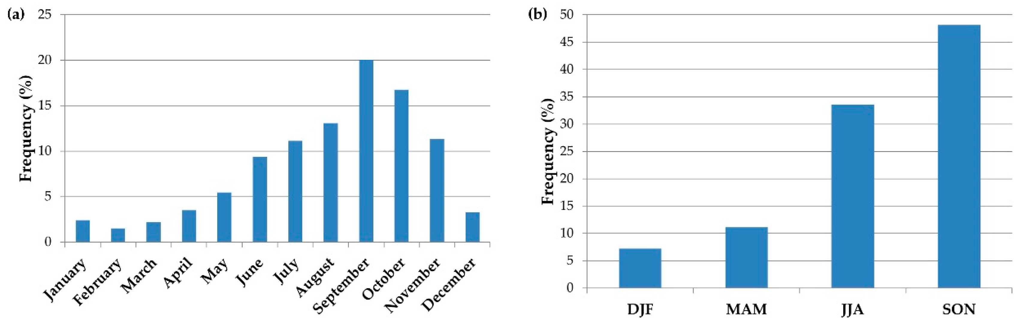
Based on the described criteria in Section 2.2, 459 events were identified in the period between 2002 and 2015. The monthly and seasonal frequency histograms are illustrated in Figure 2 (see also

Table 1. Events number for month.

MONTH	Number	%
January	11	2%
February	7	2%
March	10	2%
April	16	3%
May	25	5%
June	43	9%
July	51	11%
August	60	13%
September	92	20%
October	77	17%
November	52	11%
December	15	3%
TOTAL	459	100%

and

Table 2. Events number for season.

SEASON	Number	%
DJF	33	7%
MAM	51	11%
JJA	154	34%
SON	221	48%
TOTAL	459	100%

); it has been observed that June-July-August (JJA) and September-October-November (SON) seasons were most affected by intense events (see MetOffice classification of meteorological seasons for more details, www.metoffice.gov.uk), with a prevalence for September and October months.

These results are confirmed in several studies, e.g., [24,51]. In particular, between the last part of the summer season and the beginning of autumn, the sea surface temperature (SST) of the Mediterranean Sea reaches its maximum values. A growth for SST induces the increase of humid air, and therefore of the vertical motion of these air masses, which cause intense and abundant precipitations in contact with cooler air of the Atlantic currents. In this context, the orographic characteristics of Calabria play a crucial role: the orographic barriers (which are close to the coast) can mechanically force the motion upwards, favoring the precipitation on the windward side of the mountains.

From application of the heuristic criterion (Section 2.2), the investigated events were regrouped in Synoptic Systems (SS) and Convective Systems with Local Effects (CSLE) at the first level of analysis.

In regards to the Medicanes, from the analysis of [9,10,11,12], only three were associated with the study area in the reference period 2002–2015 (

Table 3. Tropical-Like Cyclones (TLC) characteristics.

Start	End	Max Peak (mm/20 min)	Max Peak Rain Gauge	Max Cum (mm)	Max Cum Rain Gauge
22 October 2005 18:00	23 October 2005 1:00	51.2	Molochio	224.0	Molochio
25 September 2006 22:20	27 September 2006 18:40	43.0	Monasterace—Punta Stilo	131.0	Giffone
6 November 2014 11:40	6 November 2014 12:20	25.8	Cropani	265.8	Cardeto

), which are in the list of the analyzed events by the authors. In consideration of their maximum value of cumulative rainfall, duration, and spatial extension, these three events were classified as SS.

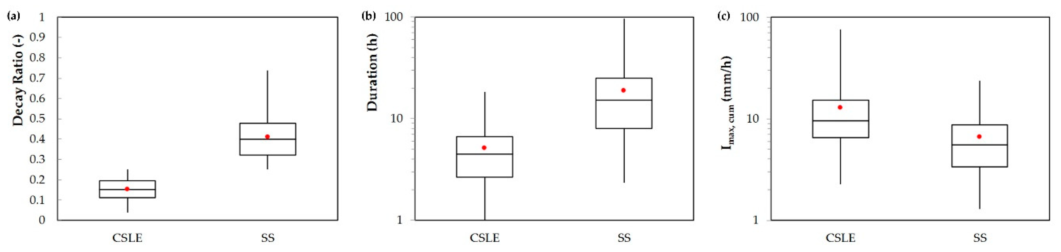
The reliability of the proposed procedure for event classification was firstly analyzed by comparing the box-plots for:

• the Decay Ratio (DR, Equation (2)), in which the authors assumed for area A a square with n = 51 km [52]. A 51-km side implies A = 2525 km²; this value should not make confusion, compared with 1000 km² (i.e., the assumed minimum extension of a strictly positive rainfall field characterizing a SS event, [5]), because two or more isolated peaks could occur inside this larger area A (i.e., a plausible situation for a CSLE event).
• Event duration d (h).
• ${\mathrm{I}}_{\max ,\mathrm{cum}}$ (mm/h), evaluated as ${\mathrm{R}}_{\max ,\mathrm{cum}}/\mathrm{d}$, i.e., the ratio between the maximum value of the observed cumulative rainfall amount and the event duration.

Figure 3a shows that the box-plots do not intersect with each other, and it seems possible to define a threshold value DR = 0.25, from which all the investigated events with DR < 0.25 can be classified as CSLE, and SS when DR > 0.25.

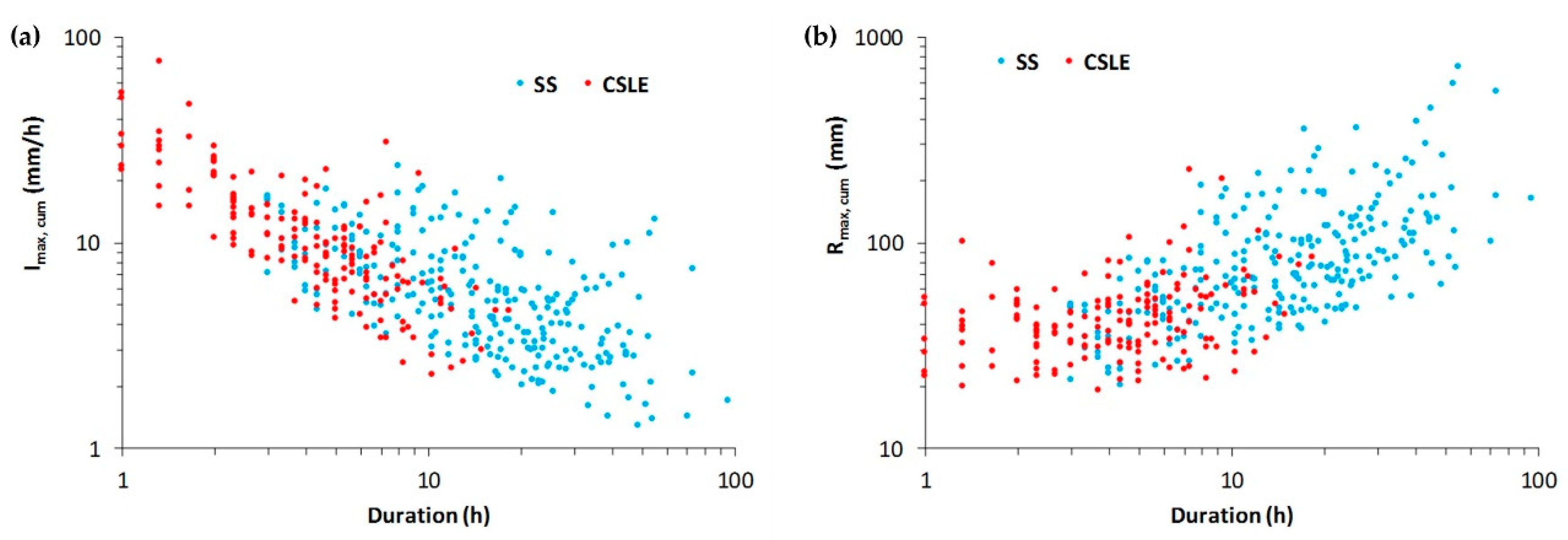
On the contrary, significant intersects can be highlighted by analyzing the box-plots for d and ${\mathrm{I}}_{\max ,\mathrm{cum}}$ (Figure 3b,c), which are also remarked in Figure 4a,b, where the authors reported the plots of ${\mathrm{I}}_{\max ,\mathrm{cum}}$ and ${\mathrm{R}}_{\max ,\mathrm{cum}}$ with respect to event duration. In detail, there are several investigated SS events that:

• are characterized by values for d and ${\mathrm{I}}_{\max ,\mathrm{cum}}$ which are representative of a CSLE event, although they present DR values > 0.25 and shapes of the rainfall field which are typical of a SS event;
• can have a very heavy value for ${\mathrm{R}}_{\max ,\mathrm{cum}}$ for large durations. In these cases, ${\mathrm{R}}_{\max ,\mathrm{cum}}$ can be equal to a significant percentage of the Mean Annual Precipitation (MAP), which is about 1000–1200 mm over the whole Calabria region [19,53].

Consequently, a second level of event classification was carried out, inside the SS group. Specifically:

• if a SS event presents values for d and ${\mathrm{I}}_{\max ,\mathrm{cum}}$ which are representative of a CSLE event or, for large durations (d > 12 h), ${\mathrm{I}}_{\max ,\mathrm{cum}}$ values greater than 140 mm/day (this is the maximum reference value in [6] for identifying an ordinary SS), that means very high values for ${\mathrm{R}}_{\max ,\mathrm{cum}}$, then it is classified as VHSS (Very Heavy Synoptic Systems);
• in the other cases, it is indicated as HSS (Heavy Synoptic Systems).

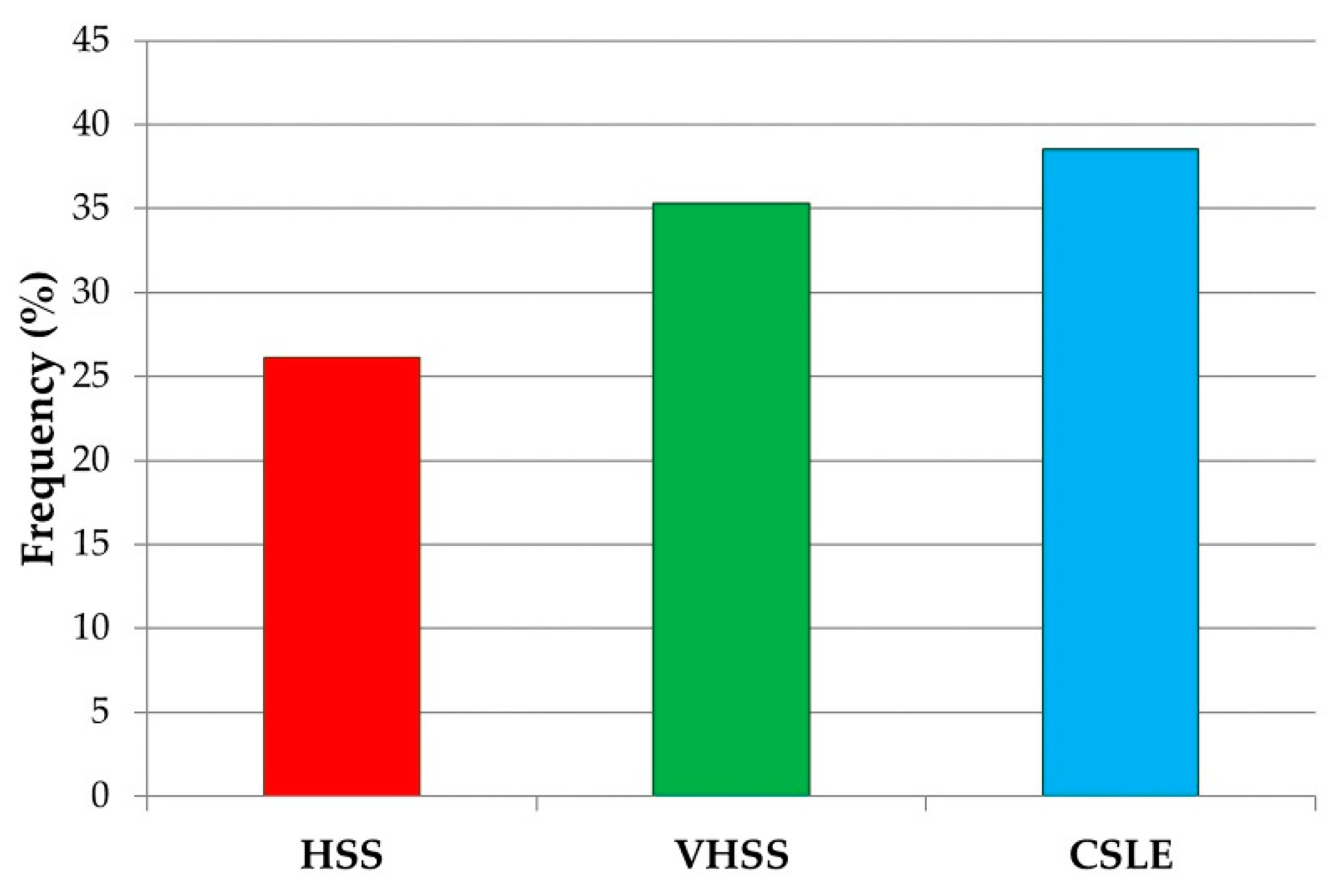
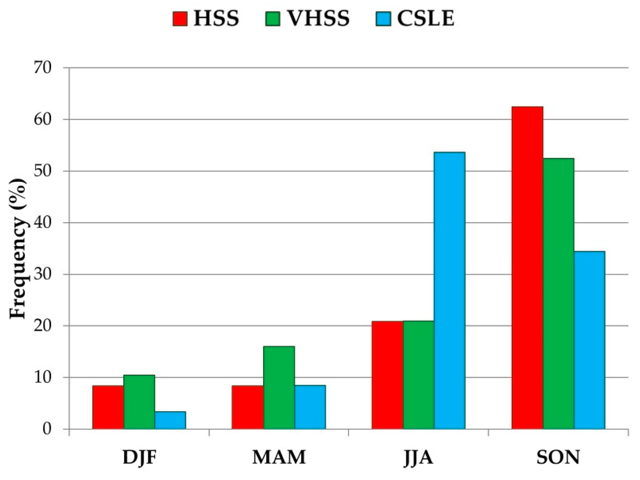
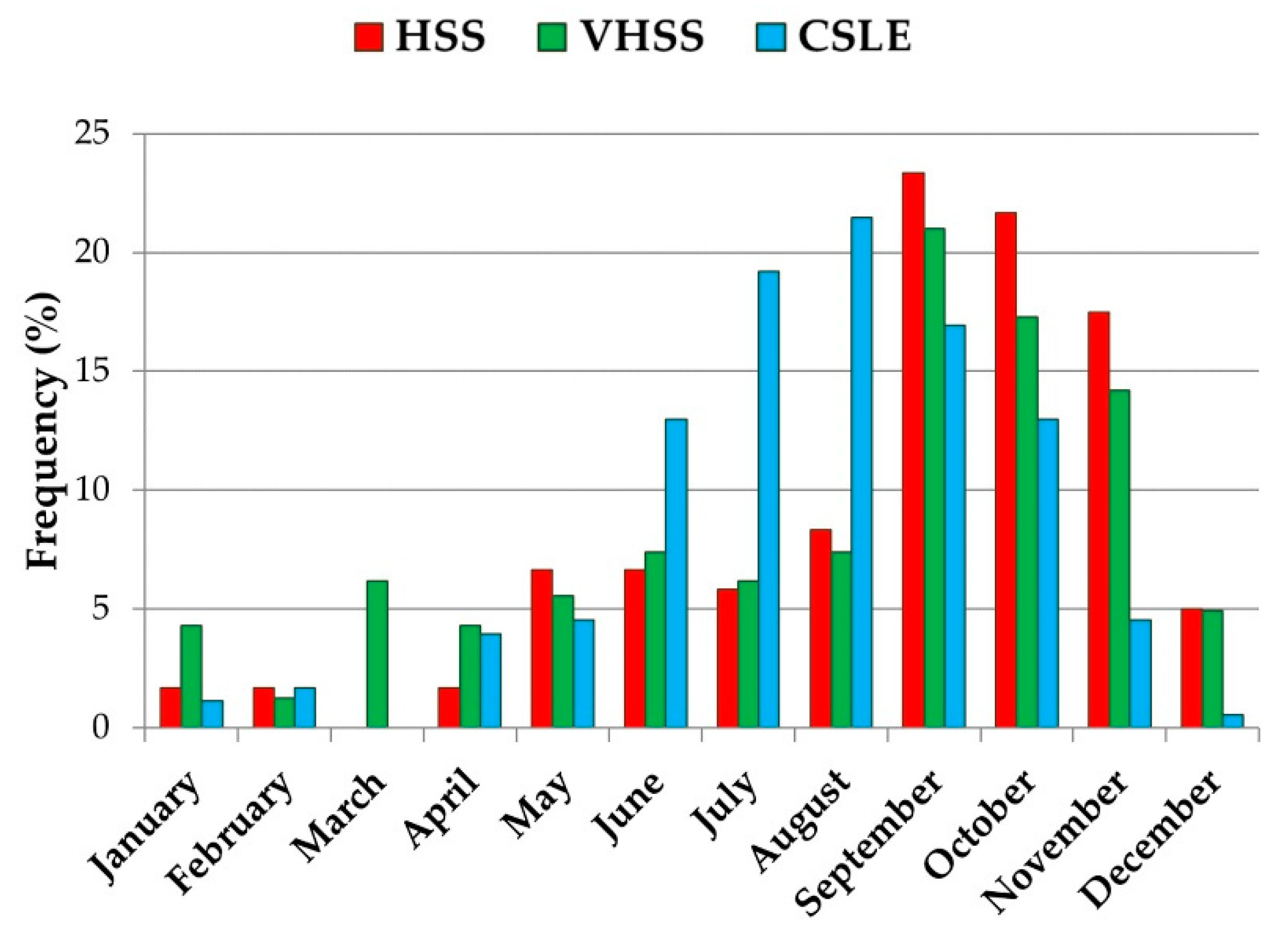
Based on this double-level classification, about 25% of the whole set of analyzed events were classified as HSS, about 35% as VHSS, and about 40% as CSLE (Figure 5). Furthermore, 63% of HSS and 52% of VHSS occurred in SON season (in particular in September and October), while more than 50% of CSLE were observed in JJA season (mainly in July and August) (Figure 6 and Figure 7).

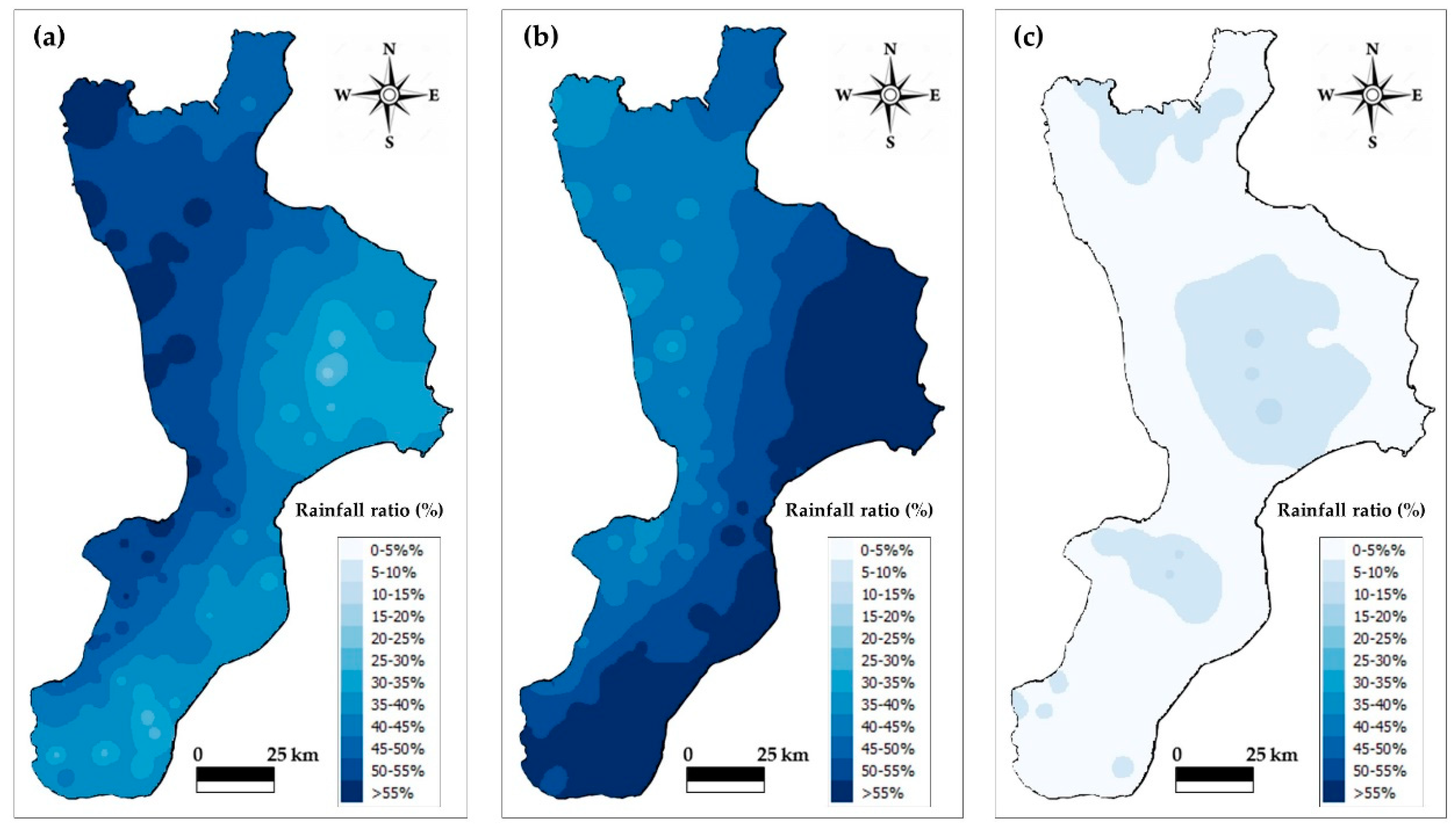
Additionally, for each rain gauge, the authors computed the ratio between the rainfall amounts related to a specific cluster and the total rainfall amounts of all the analyzed events. This ratio was then interpolated along the whole spatial domain by using the IDW method (Figure 8). HSS are characterized by percentages ranging from 22% to 65%, with higher values on the north-western coast of the region. On the contrary, the south-eastern coast of the region is mainly interested by VHSS (up to 70% of total rainfall). CSLE presented the higher percentages (however no greater than 15%) in the mountain areas (mainly in the central part of the region), which highlight the crucial role played by orographic effect for this type of events.

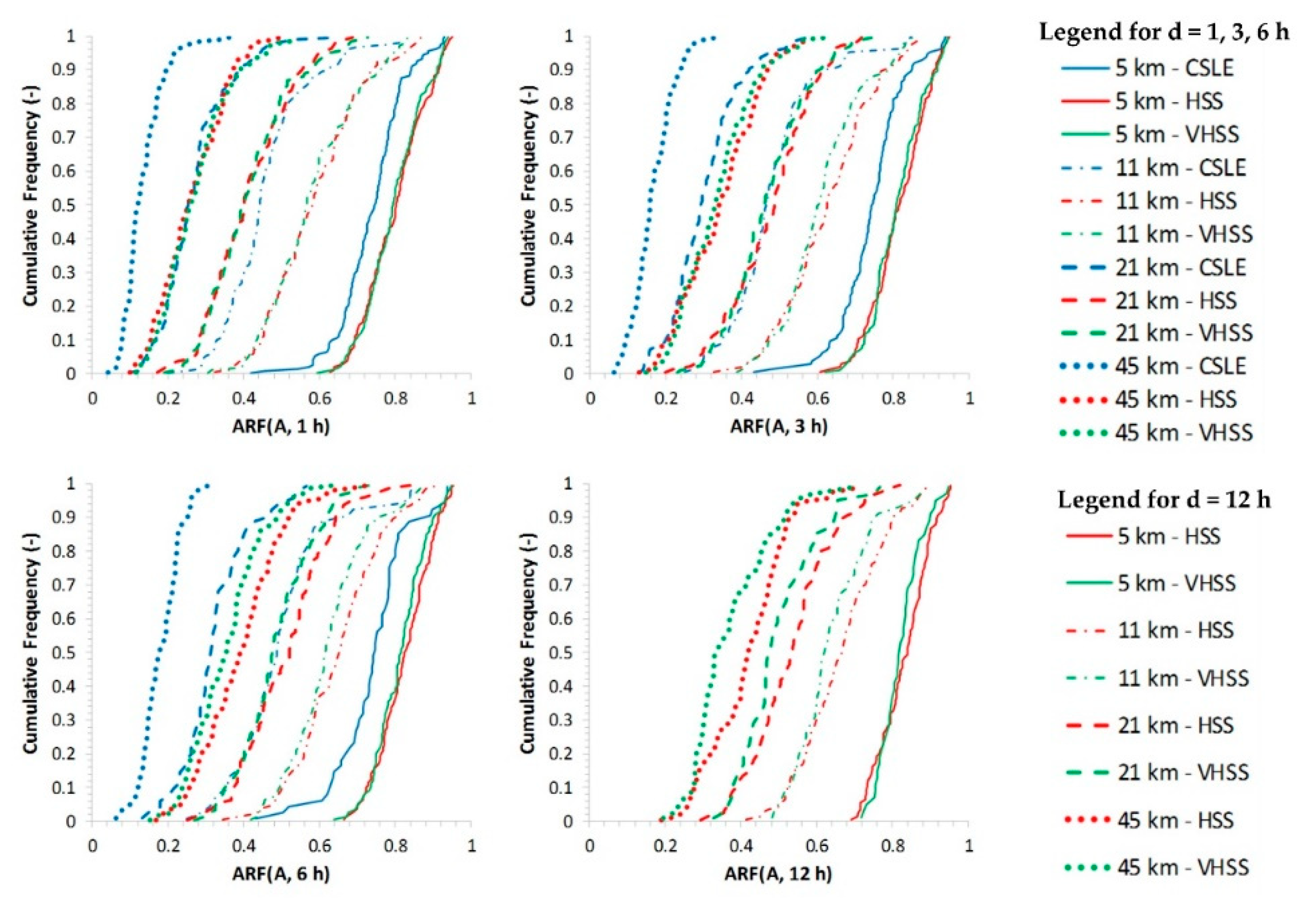
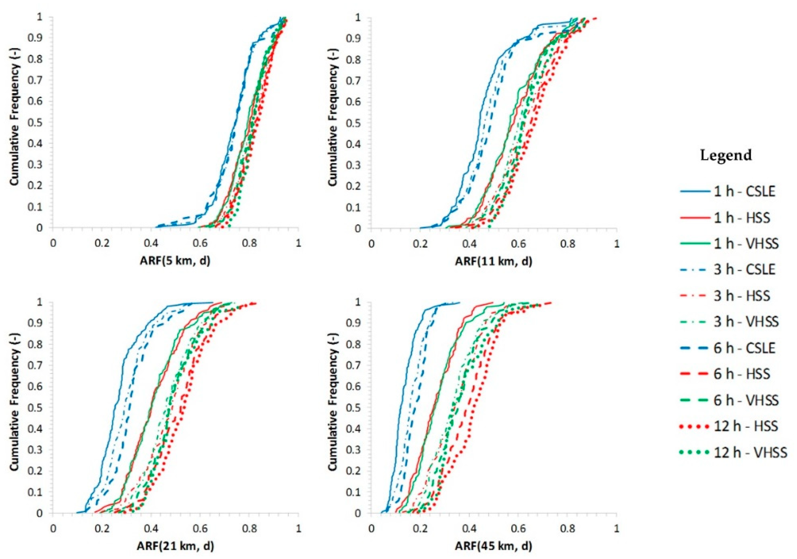
Then, for each investigated group, the authors analyzed the cumulative frequency distributions for Areal Reduction Factor (ARF, Equation (1)).

Similarly, for DR calculation, the authors considered moving nxn-pixel square grids for area A (specifically, n = 5, 11, 21 and 45 km) and moving time windows with a magnitude d = 1, 3, 6, 12 and 24 h.

Focusing on specific durations, the comparison among all the three classes was carried out until the duration of 6 h. In fact, the sample size for CSLE is not so significant for durations greater than 12 h (only six events). Moreover, the comparison between HSS and VHSS was possible until a duration of 12 h, because only 20 VHSS events present a duration greater than 24 h.

In this context, the authors investigated the influence of A, by fixing d (Figure 9), and the influence of d by fixing A (Figure 10).

Fixing the duration, each investigated value for A did not produce strong dissimilarities among the ARF distributions for HSS and VHSS; the relatively more pronounced differences are obtained when d = 12 h. In general, ARF values for HSS are slightly greater than the correspondent values for VHSS. On the contrary, CSLE distributions show marked differences from HSS and VHSS ones. In detail, ARF values for CSLE at 11 km are usually at most equal to the correspondent values for HSS and VHSS at 21 km, and this relationship is also preserved among 21-km CSLE values and 45-km HSS/VHSS.

Fixing A and varying d allow us to better graphically remark the differences among CSLE values and SS (HSS and VHSS).

3.2. ERA5 Large Scale Atmospheric Fields

As also remarked in Section 2.3, the considered ERA5 fields were: geopotential height at 500 hPa (HGT500), temperature at 850 hPa (T850), mean sea level pressure (MSLP), U and V wind component at 925 hPa (the wind components are used to calculate wind speed and direction). A domain considered representative of the synoptic characteristics mainly influencing the study area was chosen (i.e., −10° W 20° S 35° E 60° N).

Firstly, in order to evaluate the deviations of the synoptic fields associated to intense events with respect to the whole considered 14-year period, the ERA5 fields were extracted at 12 UTC of each day. In detail, a statistical sample covering 5113 days was obtained, and the mean values were computed for the all the parameters defined above.

For the successive analysis, the authors focused on the most severe heavy events from the ensemble of the selected 459 events, which represent a topic of increasing interest for the scientific community [13,14,15]. In detail, for each class (CSLE, HSS and VHSS) and starting from the frequency distributions for (i) the maximum intensity in 20 min, (ii) I_{max, cum}, (iii) R_{max, cum} in each class, the authors considered:

• the events which are greater than the sample 90% percentile in at-least one distribution and then;
• from this previous filter, heavy rain events with at least 60 mm in 24 h [54], observed in one rain gauge.

Based on these conditions, the number of events was reduced from 459 to 67 (see

Table A1. List of the selected Most Heavy Rain (MHR) events.

Start	End	Max Peak (mm/20 min)	Max Peak Rain Gauge	Max Cum (mm)	Max Cum Rain Gauge
2 September 2002 12:00	2 September 2002 18:40	36.4	Tiriolo	118.4	Tiriolo
27 September 2003 14:00	27 September 2003 15:20	22.0	Staiti	78.4	Staiti
14 October 2003 12:40	15 October 2003 18:00	38.0	Petronà	237.0	Petronà
29 October 2003 23:20	30 October 2003 17:20	36.4	Lagonegro	95.2	Lagonegro
22 November 2003 3:20	22 November 2003 11:00	27.0	San Luca—Santuario di Polsi	139.2	Santa Cristina d’Aspromonte
11 December 2003 0:00	13 December 2003 4:40	28.6	Antonimina—Canolo Nuovo	588.2	San Luca—Santuario di Polsi
3 June 2004 7:00	3 June 2004 11:20	17.8	C.le Castrocucco	105.6	C.le Castrocucco
20 September 2004 2:40	21 September 2004 1:20	42.0	Cropalati	137.4	Monasterace—Punta Stilo
3 November 2004 14:40	5 November 2004 8:20	27.8	Tarsia	165.0	Tarsia
12 November 2004 11:40	13 November 2004 5:20	41.6	Decollatura	222.4	Parenti
6 September 2005 13:00	6 September 2005 16:40	28.6	Arena	80.6	Arena
22 October 2005 18:00	23 October 2005 1:00	51.2	Molochio	224.0	Molochio
2 January 2006 1:00	2 January 2006 6:00	47.4	Lagonegro	70.2	Lagonegro
3 July 2006 5:00	3 July 2006 14:00	45.0	Vibo Valentia	202.6	Vibo Valentia
8 July 2006 12:40	8 July 2006 18:00	35.2	Roccabernarda—Serrarossa	69.6	Serra San Bruno
25 September 2006 22:20	27 September 2006 18:40	43.0	Monasterace—Punta Stilo	131.0	Giffone
22 December 2006 2:00	23 December 2006 16:40	24.6	Palermiti	243.2	Corigliano Calabro
27 May 2007 21:40	28 May 2007 11:20	33.4	Gioia Tauro	78.8	Castrovillari—Camerata
7 October 2007 1:40	7 October 2007 17:20	30.0	Belvedere Marittimo	103.0	Belvedere Marittimo
28 October 2008 18:40	28 October 2008 23:00	56.8	Gioiosa Ionica	84.0	Gioiosa Ionica
07 November 2008 4:20	07 November 2008 9:20	18.6	Stignano	81.0	Stignano
28 November 2008 12:40	28 November 2008 22:00	21.2	Antonimina—Canolo Nuovo	180.4	Petilia Policastro—Pagliarelle
03 December 2008 16:20	03 December 2008 12:20	20.0	Stignano	120.4	Cropalati
10 December 2008 13:40	12 December 2008 5:40	23.0	Spineto	389.2	Santa Cristina d’Aspromonte
9 January 2009 15:40	10 January 2009 0:40	25.4	Corigliano Calabro	165.8	Corigliano Calabro
13 January 2009 3:20	13 January 2009 22:20	21.2	Santa Cristina d’Aspromonte	283.8	Santa Cristina d’Aspromonte
21 September 2009 23:20	23 September 2009 18:20	30.0	Santa Caterina dello Ionio	301.6	Santa Caterina dello Ionio
24 September 2009 13:40	27 September 2009 14:40	42.6	Chiaravalle Centrale	544.0	Petronà
23 October 2009 16:00	25 October 2009 12:20	43.4	Monasterace—Punta Stilo	126.2	Monasterace—Punta Stilo
10 November 2009 14:00	11 November 2009 22:40	16.8	Rosarno	193.0	Rosarno
14 December 2009 8:20	15 December 2009 4:40	16.0	Santa Cristina d’Aspromonte	119.6	Santa Cristina d’Aspromonte
26 January 2010 18:40	27 January 2010 20:00	25.0	Plati’	360.0	Fabrizia—Cassari
9 March 2010 16:20	10 March 2010 10:40	21.4	Cropani	260.8	Cotronei
03 September 2010 4:40	04 September 2010 10:00	40.8	Reggio Calabria	155.0	San Mauro Marchesato
6 October 2010 5:40	6 October 2010 23:20	20.8	Laino Borgo	101.8	Laino Borgo
18 October 2010 12:20	19 October 2010 20:20	30.4	Bagnara Calabra	218.0	Serralta
2 November 2010 8:20	2 November 2010 16:00	25.2	Gambarie d’Aspromonte	188.6	Rizziconi
14 October 2011 8:40	15 October 2011 5:00	39.2	Ciro’ Marina—Punta Alice	67.6	Sant’Agata del Bianco
23 October 2011 4:20	23 October 2011 18:20	25.6	Cariati Marina	85.0	Cariati Marina
11 November 2011 14:40	12 November 2011 2:40	26.8	Scilla—Tagli	114.2	Scilla—Solano
22 November 2011 10:00	23 November 2011 3:00	43.8	Cittanova	353.4	Cittanova
23 July 2012 20:00	24 July 2012 3:40	36.8	Oriolo	89.0	Oriolo
13 September 2012 11:40	15 September 2012 2:00	37.6	Cetraro Superiore	142.2	Cetraro Superiore
15 November 2012 12:00	16 November 2012 18:00	21.4	Monasterace—Punta Stilo	168.2	Santa Caterina dello Ionio
17 November 2012 0:40	18 November 2012 22:20	27.0	Ciro’ Marina—Punta Alice	167.4	Palermiti
19 November 2012 12:20	21 November 2012 16:20	17.6	Roseto Capo Spulico	182.8	Rosarno
8 July 2013 11:00	8 July 2013 16:40	28.8	San Sosti	71.2	Nocelle—Arvo
7 October 2013 9:00	7 October 2013 15:00	34.4	San Mauro Marchesato	99.2	San Mauro Marchesato
8 October 2013 13:00	8 October 2013 18:40	30.6	Ciro’ Marina—Punta Alice	71.4	Ciro’ Marina—Punta Alice
15 October 2013 23:20	16 October 2013 22:40	39.2	Palermiti	90.4	Serralta
12 November 2013 20:40	14 November 2013 12:00	30.6	Soverato Marina	109.6	Chiaravalle Centrale
15 November 2013 12:40	16 November 2013 17:20	22.6	Borgia— Roccelletta	146.0	Cerenzia
18 November 2013 23:00	19 November 2013 11:00	38.4	Serra San Bruno	215.2	Ciro’ Marina—Punta Alice
31 January 2014 18:00	2 February 2014 14:40	23.2	Palermiti	447.6	Petilia Policastro—Pagliarelle
21 February 2014 4:20	21 February 2014 7:20	22.0	Scilla—Tagli	70.2	Scilla—Tagli
1 September 2014 16:00	2 September 2014 9:40	22.6	Vibo Valentia—Longobardi	106.2	Sinopoli
13 September 2014 4:00	13 September 2014 8:00	39.0	Belvedere Marittimo	66.4	Belvedere Marittimo
4 November 2014 21:00	5 November 2014 23:00	45.4	Roccella Ionica	271.4	Plati’
6 November 2014 11:40	8 November 2014 12:20	25.8	Cropani	265.8	Cardeto
21 June 2015 10:00	21 June 2015 20:40	19.4	Mongiana	73.2	Mongiana
9 August 2015 12:00	9 August 2015 16:00	29.2	Arena	80.4	Arena
11 August 2015 10:00	12 August 2015 23:00	39.4	Oriolo	255.2	Corigliano Calabro
13 August 2015 13:20	13 August 2015 14:20	39.2	Plati’	100.8	Plati’
20 September 2015 11:20	21 September 2015 7:00	37.2	Antonimina—Canolo Nuovo	176.0	Antonimina—Canolo Nuovo
7 October 2015 6:40	7 October 2015 18:00	38.4	Tortora	67.6	San Sosti
20 October 2015 13:00	20 October 2015 20:00	17.4	Ciro’ Marina—Punta Alice	91.4	Ciro’ Marina—Punta Alice
30 October 2015 19:20	2 November 2015 2:00	30.2	Ardore Superiore	717.2	Chiaravalle Centrale

in Appendix A), which were indicated as Most Heavy Rain (MHR) events: 20 of these are HSS, 28 are VHSS and 19 are CSLE. In general, analysis of MHR events clearly plays a crucial role in many contexts, in particular for Civil Protection purposes.

With an a-posteriori analysis, the authors verified that all the most significant events occurred in Calabria in recent years. Moreover, many of these were also studied both by the Multi Risks Center of Calabria region (see the dedicated web page, in Italian language, where several technical reports are listed: http://www.cfd.calabria.it/index.php/pubblicazioni/voce-2; last access 5 April 2020) and by the scientific community (e.g., “the Vibo Valentia case” [55]; “the October-November 2015 case” [23,56]). This confirms the validity of the adopted method, aimed at selecting the most significant rainfall events that occurred in the region.

For each MHR, the related averaged large-scale atmospheric patterns were analysed, taking into account the values of the large-scale fields at 12 UTC of the day before the events themselves.

Upon the events, the ERA5 fields were averaged for the three identified classes (HSS, VHSS and CSLE respectively), with the aim of generating three representative large-scale scenarios.

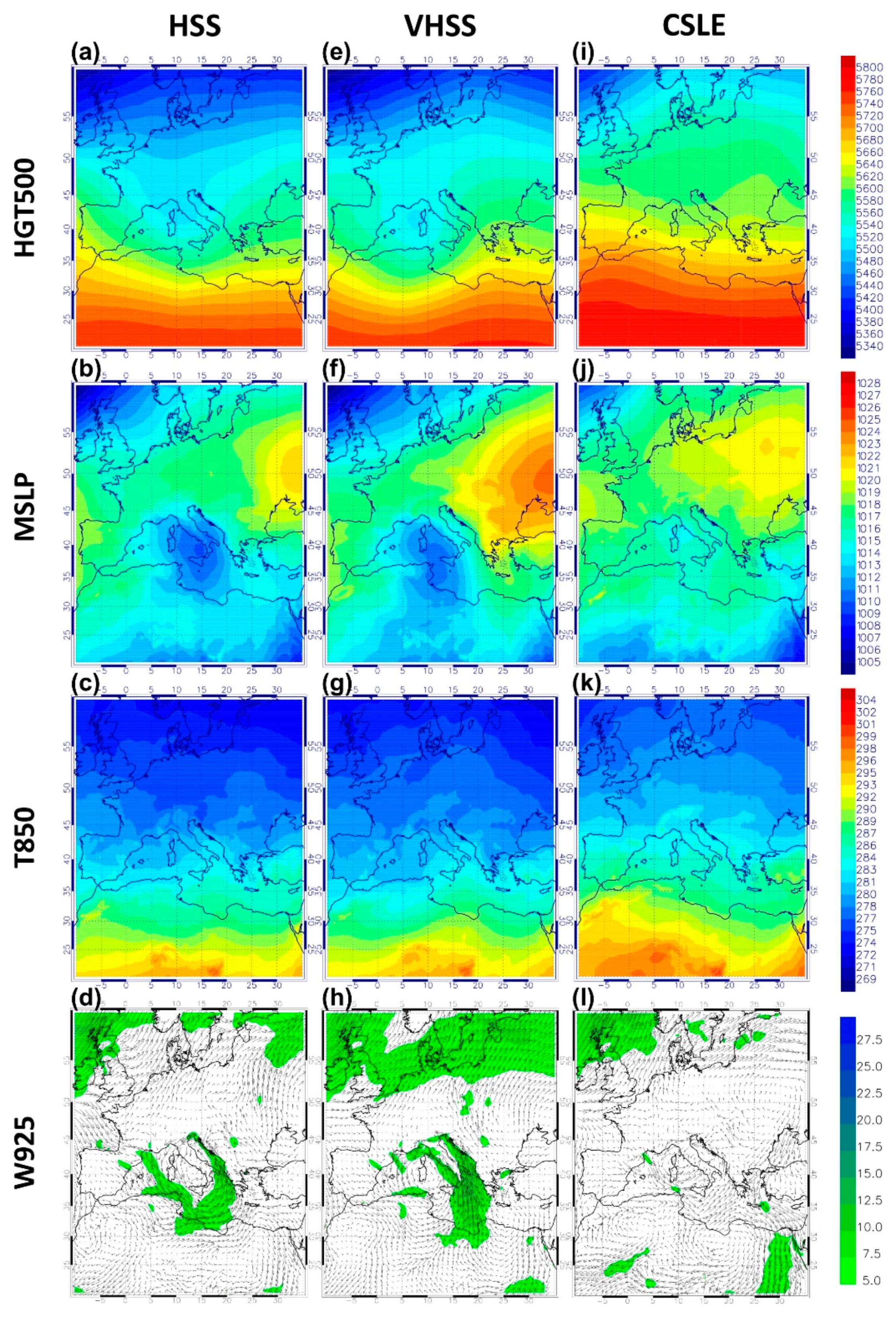
In Figure 11 (multi-panel 4 rows × 3 columns) the following fields are showed: HGT500 (first row), MSLP (second row), T850 (third row) and wind (direction and speed; fourth row) at 925 hPa respectively. These fields are the result of the average made for HSS (first column), for VHSS (second column) and for CSLE (third column).

The computed 14-year averaged fields are not here reported for brevity, but they were taken into account to evaluate (see Figure 12) the anomalies with respect to the average of the specific cases and, therefore, to highlight specific indicators plausible related to the phenomena occurring in the three classes of events.

3.3. Heavy Synoptic Systems (HSS)

In the HSS case, it can be seen that the northern Italy and the northern Tyrrhenian are affected by an upper-level trough, as regards the average value of the HGT500 (Figure 11a). This is indicative of the presence of cold air at the medium layers descending from the central Europe (Figure 11c), and to which corresponds a pronounced low pressure at the surface (Figure 11b).

This situation facilitates the coming of North-Atlantic currents passing through the Rhone valley into the Mediterranean area; these currents appear subsequently deviated by the low and assume a south-western orientation over southern Italy. By observing the average low-level wind field for the HSS case (Figure 11d), it is evident the presence of currents with cyclonic circulation in the Mediterranean. In particular, it is noteworthy a distinction between the north-western currents over the western Tyrrhenian Sea and the south-western currents over the Ionian Sea, and rising on the Adriatic Sea.

In this context, the Calabria region is interested by a low-pressure core and, therefore, the prevailing currents are highly variable and directed (on average) from south-west. The averaged wind values, around the identified low, are between 5 and 10 m/s (green colours in Figure 11d).

3.4. Very Heavy Synoptic Systems (VHSS)

The differences between the VHSS case (second column) and the HSS case discussed above are apparently minimal.

In this case, the upper-level trough appears (Figure 11e) more displaced to West; in fact, the system is now centred between Sardinia/Corsica and the Balearics.

On the surface, this corresponds to the presence of a low-pressure area, which is very similar to that highlighted in the HSS case but more westward, therefore completely extended over the Mediterranean Sea (Figure 11f). Although this does not show significant differences in terms of temperature at about 1500 m (Figure 11g), substantial differences are perceived by observing the mean low-level wind field (Figure 11h). In this case, the cyclonic circulation is also evident compared to the previous case but, being more displaced towards the west, the averaged currents affecting southern Italy are coming from S-SE and appear more intense (locally > 10 m/s).

In such conditions, the disturbances affecting Calabria are most linked to the advection of hot and unstable (maritime in particular) air.

Compared to HSS, VHSS cases are characterized by less extended events which, however, have greater intensity, especially due to the more unstable nature of the air masses of a distinctly maritime nature. This occurrence is confirmed by the climatology of the main disturbance affecting Calabria and it is in agreement with the results obtained by [20]: the most intense rainstorms mainly affect the east side, which is favourably exposed to these storms, although cumulative precipitation is larger on the west side of the Calabria.

3.5. Convective Systems with Local Effects (CSLE)

As previously seen, these are mostly summer events. From a synoptic point of view, only an upper-level ridge is visible over north-western Africa at 500 hPa (Figure 11i). In these circumstances, high-level currents are facilitated to flow from SW to the Tyrrhenian coast of Calabria.

On the surface, there are no significant baric gradients, although a depression area on the northern Tyrrhenian is visible (Figure 11j). This suggests that the events are connected to local phenomena and are caused by short-lived forcing, and therefore they are less affected by the more organized large-scale patterns. In such circumstances, the development of convection and atmospheric instability plays a role of primary importance.

The temperature at 850 hPa is generally higher than in previous cases (HSS and VHSS). The presence of warmer air on the central Mediterranean basin is evident (Figure 11k). Differences up to 5 K are visible over the sea, and about 3 K over Calabria. The warmer air facilitates the development of instability and convection in the areas surrounding the Calabria region. Near surface winds are weaker than in previous cases and meanly oriented from west (Figure 11l).

3.6. Analysis of Anomalies

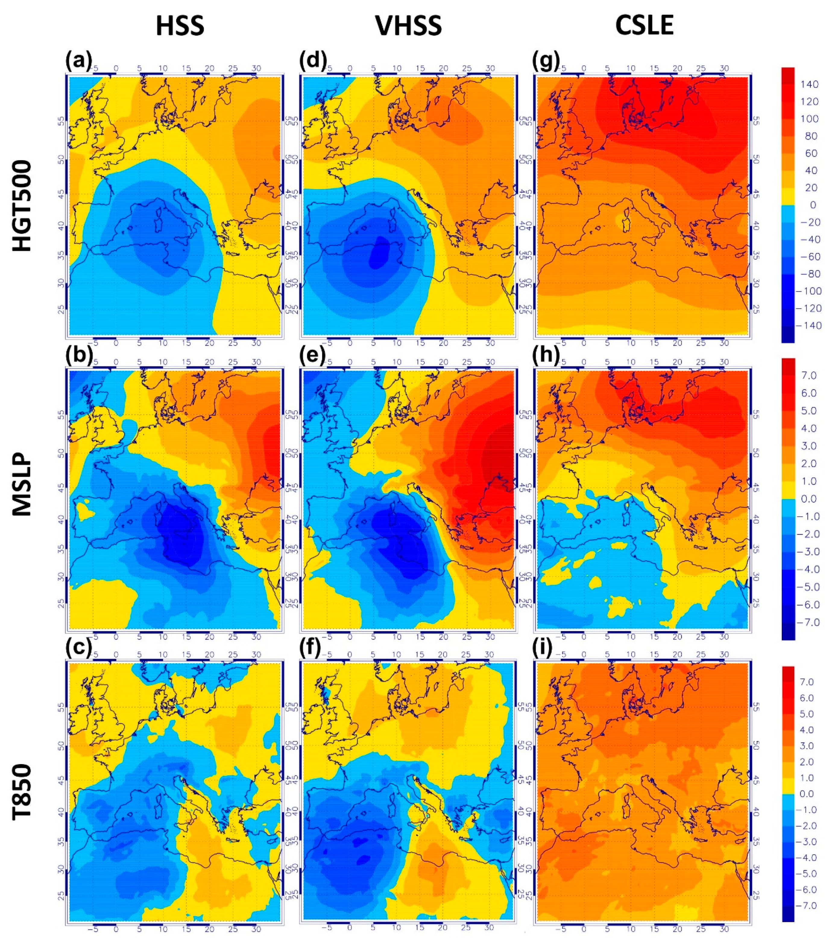
In order to highlight the anomalies of the large-scale patterns with respect to the average, Figure 12 (multi-panel 3 rows × 3 columns) shows the differences between the averaged fields (HGT500 first row, MSLP second row, T850 third row) for HSS (first column), for VHSS (second column), and for CSLE (third column) with respect to the whole considered period of 14 years.

If Figure 11 can be useful to quantify the averaged synoptic fields during the extreme events, then Figure 12 is even more intuitive in defining specific areas where anomalies of pressure, temperature and geopotential height occurred.

From these comparisons, it is possible to outline large-scale predictive indicators which are potentially able to provide prognostic information, in order to evaluate the role of the considered synoptic parameters as possible precursors. These “anomaly-fields” can be considered as indicative benchmarks on Mediterranean area, also in the perspective of climate change and for the potential effects associated with it.

Colours in blue (red) scale indicate negative (positive) values and therefore negative (positive) anomalies of the considered fields; therefore, the values of the fields are lower (higher) than the average in these areas.

By observing the first and second columns of Figure 12, relating to HSS and VHSS cases, it can be assessed that these events are characterized by lower than average geopotential height values (up to −80, Figure 12d) in the central-western Mediterranean and north-western Africa, corresponding to a negative surface pressure anomaly (Figure 12, second row). The consequences of these anomalies, in terms of flows, are further accentuated by the positive anomalies of HGT500 and MSLP on central-eastern Europe.

It is interesting to observe the deviation from the average of the temperature at about 1500 m (Figure 12c,f). An area with temperature values which are lower than the average one (up to 4 degrees) is evident in the north-western African regions; there are equally apparent small deviations from the average (positive anomaly) in the north-eastern African areas (up to 3 degrees) and in central-eastern Europe (locally up to 5 degrees).

The HSS (Figure 12, first column) and the VHSS (Figure 12, second column), as seen in the previous comments, have very similar behaviours. VHSS present more pronounced gradients that are more shifted towards the west; this occurrence, as seen, is the basis of the different (in direction and magnitude) currents that impact the southern Italy regions.

Considering the MSLP, for example for the specific case of VHSS (Figure 12e), it is possible to note a deviation from the average up to −6 mb on the surface pressure, on the entire Mediterranean area. A wide area corresponds to this negative anomaly, in central and eastern Europe, with surface pressure values up to +8 mb higher than the average values.

An omega structure with an inclined axis with NW-SE orientation is clearly visible, especially for the surface pressure fields (Figure 12, second row), but also for HGT500 (Figure 12, first row). The oscillation of this dipolar structure (both in terms of mutual position and magnitude), very similar in form to that relating to the well-known index such as NAO (North Atlantic Oscillation), determines (like the index mentioned above) the trajectories and intensities of the Atlantic disturbances affecting the Mediterranean.

As we can expect, the anomalies relating to the CSLE cases are much less evident than in the previous cases, being more isolated events and less linked to synoptic patterns.

At about 5500 m, the anomaly is slightly positive everywhere (Figure 12g), while on the surface (MSLP, Figure 12h) there is a slight negative anomaly of pressure on the central-western Mediterranean and on the north-western African regions.

It is interesting to note, for this case, the behaviour of the T850 (Figure 12i) which shows a positive anomaly on the entire domain that is indicative of a warmer environment everywhere, up to 3 degrees in some zones. This situation facilitates the development of convective motions and, therefore, of vertical instability, often on the basis of localized intense phenomena (i.e., summer storms).

4. Discussion

The overall obtained results remark the importance of an in-depth analysis of high-resolution rain gauge data (in terms of visual inspection of the rainfall fields and then by analysing specific features), in order to better classify the main precipitations systems associated to extreme events for an assigned study area.

In detail, the areal reduction factor represents an important discriminant between CSLE and SS for Calabria region, while it is not so significant to separate SS events in VHSS and HSS, for which intensity, duration and cumulative rainfall values are more suitable.

The analysis of large-scale modelling products allows for better explaining the study with ground data. Specifically, two main points can be highlighted:

• the investigated synoptic systems are mainly characterized by negative anomalies for geopotential height (between −80 and −100 m) and sea level pressure (up to −6 hPa) in the central-western Mediterranean. For the VHSS, the region of greatest anomaly is more displaced to west respect to HSS, and the low-level winds reach Calabria region coming from S-SE, facilitating the development of favourable conditions for heaviest rainfall on the eastern side of the region. In the HSS case the rainfall is favoured on the western coast of the region, in agreement with the observations (Figure 8a,b);
• the investigated convective systems are predominantly related to the low-level temperature that presents a positive anomaly everywhere (locally up to 3 K), causing localized convection development and major rainfall in correspondence of the orographic reliefs (Figure 8c).

In general, this coupled analysis (ground data with large-scale modelling products) can clearly permit to obtain noticeable improvements in many related topics, from nowcasting models to the definition of design rainfall scenarios in space and time, with consequent progress for evaluation of risk scenarios associated to induced phenomena (mainly floods and landslides).

5. Conclusions

In this work, an integrated analysis was proposed, including datasets from rain gauge network and ECMWF-ERA5 Reanalysis, in order to select the main synoptic fields which can be considered as possible precursors of the intense precipitation events.

The selection and the classification of heavy rainfall events from rain gauge data for Calabria region (southern Italy) allowed to highlight the crucial role played by:

• Areal Reduction Factors (ARFs) for numerically characterizing the differences in scaling (in space and time) between Convective Systems with Local Effects (CSLE) and Synoptic Systems (SS);
• Rainfall Intensity and Cumulative Rainfall amounts for furtherly discriminating Very Heavy Synoptic Systems (VHSS) from Heavy Synoptic Systems (HSS).

The major part of SS usually occurred in SON season (in particular in September and October); HSS events mainly interested the north-western coast of the region, while VHSS events mostly regarded the south-eastern coast of Calabria. More than 50% of CSLE were observed in JJA season (mainly in July and August), and in the mountain areas, mainly in the central part of the region, which highlight the crucial role played by orographic effect for this type of events.

Considering the ERA5 atmospheric fields, it was possible to obtain some useful indicators linked to the main rainfall patterns. In particular, the authors focused attention on the Most Heavy Rainfall events (MHR) from the ensemble of the selected 459 events, which are of increasing interest for the scientific community and for Civil Protection purposes.

For the SS group, further classified in HSS and VHSS, a key role is played by the position of the averaged low-pressure area over the Mediterranean. For the VHSS cases, the low (as well as the corresponding upper level trough) appears more displaced to West; this implies considerable differences in the mean low-level wind field that is more intense and affects southern Italy coming from S-SE, facilitating the advection of moister and hotter maritime air towards the coasts of the Calabria region. With respect to HSS, VHSS cases are characterized by events with less spatial extent but greater intensity, in agreement with the available literature on the climatology of extreme rainfall events in southern Italy.

For the CSLE group, the most important atmospheric parameter seems to be the temperature. In this case, no significant baric gradients are visible but the averaged low-level temperature is higher than in previous cases. The warmer air facilitates the development of convection and atmospheric instability.

As also remarked in the Introduction, the proposed analysis should not be considered alternative to the use of mesoscale Numerical Weather Prediction models, but as a survey able to provide useful information about the rainfall patterns and the related synoptic fields, particularly suitable for the definition of the prevalent heavy-rain scenarios in Mediterranean and for risk mitigation analysis.

References

- Houze, R.A., Jr. Structures of atmospheric precipitation systems—A global survey. Radio Sci. 1981, 16, 671–689. [Google Scholar] [CrossRef]
- De Luca, C.; Furcolo, P.; Rossi, F.; Villani, P.; Vitolo, C. Extreme Rainfall in Mediterranean. In Proceedings of the STAHY 2010 International Workshop Advances In Statistical Hydrology, Taormina, Italy, 23–25 May 2010. [Google Scholar]
- Ulbrich, U.; Lionello, P.; Belusic, D.; Jacobeit, J.; Knippertz, P.; Kuglitsch, F.G.; Leckebusch, G.C.; Luterbacher, J.; Maugeri, M.; Maheras, P.; et al. Climate of the Mediterranean: Synoptic Patterns, Temperature, Precipitation, Winds, and Their Extremes. In Climate of the Mediterranean Region—From the Past to the Future; Lionello, P., Ed.; Elsevier: Sydney, Australia, 2012; Volume 5, pp. 301–346. [Google Scholar] [CrossRef]
- Lionello, P.; Trigo, I.F.; Gil, V.; Liberato, M.L.R.; Nissen, K.M.; Pinto, J.G.; Raible, C.C.; Reale, M.; Tanzarella, A.; Trigo, M.R.; et al. Objective climatology of cyclones in the Mediterranean region: A consensus view among methods with different system identification and tracking criteria. Tellus A 2016, 68, 29391. [Google Scholar] [CrossRef] [Green Version]
- Willems, P. A spatial rainfall generator for small spatial scales. J. Hydrol. 2001, 252, 126–144. [Google Scholar] [CrossRef]
- Rossi, F.; Scannapieco, G.; Villani, P. Una proposta operativa per la rivalutazione del rischio idrogeologico di alluvione in Italia (in Italian). In Proceedings of the XXXV Convegno di Idraulica e Costruzioni Idrauliche, Bologna, Italy, 14–16 September 2016. [Google Scholar]
- Waymire, E.; Gupta, V.K.; Rodriguez-Iturbe, I. A spectral theory of rainfall intensity at the meso-b scale. Water Resour. Res. 1984, 20, 1453–1465. [Google Scholar] [CrossRef]
- Reale, O.; Atlas, R. Tropical Cyclone–Like Vortices in the Extratropics: Observational Evidence and Synoptic Analysis. Weather Forecast. 2001, 16, 7–34. [Google Scholar] [CrossRef]
- Tous, M.; Romero, R. Medicanes: Cataloguing criteria and exploration of meteorological environments. Tethys 2011, 8, 53–61. [Google Scholar] [CrossRef]
- Tous, M.; Romero, R. Meteorological environments associated with medicane development. Int. J. Clim. 2012, 33, 1–14. [Google Scholar] [CrossRef]
- Cavicchia, L.; Von Storch, H. The simulation of medicanes in a high-resolution regional climate model. Clim. Dyn. 2011, 39, 2273–2290. [Google Scholar] [CrossRef]
- Miglietta, M.M.; Laviola, S.; Malvaldi, A.; Conte, D.; Levizzani, V.; Prince, C. Analysis of tropical-like cyclones over the Mediterranean sea through a combined modeling and satellite approach. Geophys. Res. Lett. 2013, 40, 2400–2405. [Google Scholar] [CrossRef]
- Pelosi, A.; Furcolo, P.; Rossi, F.; Villani, P. The characterization of extraordinary extreme events (EEEs) for the assessment of design rainfall depths with high return periods. Hydrol. Process. 2020. [Google Scholar] [CrossRef]
- Libertino, A.; Ganora, D.; Claps, P. Technical note: Space-time analysis of rainfall extremes in Italy: Clues from a reconciled dataset. Hydrol. Earth Syst. Sci. 2018, 22, 2705–2715. [Google Scholar] [CrossRef] [Green Version]
- Castellarin, A.; Merz, R.; Blöschl, G. Probabilistic envelope curves for extreme rainfall events. J. Hydrol. 2009, 378, 263–271. [Google Scholar] [CrossRef]
- Lana, A.; Campins, J.; Genovés, A.; Jansà, A. Atmospheric patterns for heavy rain events in the Balearic Islands. Adv. Geosci. 2007, 12, 27–32. [Google Scholar] [CrossRef] [Green Version]
- Martínez, C.; Campins, J.; Jansà, A.; Genovés, A. Heavy rain events in the Western Mediterranean: An atmospheric pattern classification. Adv. Sci. Res. 2008, 2, 61–64. [Google Scholar] [CrossRef] [Green Version]
- Romero, R.; Ramis, C.; Alonso, S.; Doswell, C.A., III; Stensrud, D.J. Mesoscale Model Simulations of Three Heavy Precipitation Events in the Western Mediterranean Region. Mon. Weather Rev. 1998, 126, 1859–1881. [Google Scholar] [CrossRef]
- Llasat, M.C.; Llasat-Botija, M.; Petrucci, O.; Pasqua, A.A.; Rosselló, J.; Vinet, F.; Boissier, L. Towards a database on societal impact of Mediterranean floods within the framework of the HYMEX project. Nat. Hazards Earth Syst. Sci. 2013, 13, 1337–1350. [Google Scholar] [CrossRef] [Green Version]
- Federico, S.; Avolio, E.; Pasqualoni, L.; De Leo, L.; Sempreviva, A.M.; Bellecci, C. Preliminary results of a 30-year daily rainfall data base in southern Italy. Atmos. Res. 2009, 94, 641–651. [Google Scholar] [CrossRef]
- Federico, S.; Pasqualoni, L.; Avolio, E.; Bellecci, C. Brief communication “Calabria daily rainfall from 1970 to 2006”. Nat. Hazards Earth Syst. Sci. 2010, 10, 717–722. [Google Scholar] [CrossRef]
- Avolio, E.; Federico, S.; Miglietta, M.M.; Lo Feudo, T.; Calidonna, C.R.; Sempreviva, A.M. Sensitivity analysis of WRF model PBL schemes in simulating boundary-layer variables in southern Italy: An experimental campaign. Atmos. Res. 2017, 192, 58–71. [Google Scholar] [CrossRef]
- Avolio, E.; Federico, S. WRF simulations for a heavy rainfall event in southern Italy: Verification and sensitivity tests. Atmos. Res. 2018, 209, 14–35. [Google Scholar] [CrossRef]
- Federico, S.; Avolio, E.; Pasqualoni, L.; Bellecci, C. Atmospheric patterns for heavy rain events in Calabria. Nat. Hazards Earth Syst. Sci. 2008, 8, 1173–1186. [Google Scholar] [CrossRef] [Green Version]
- Pielke, R.A.; Cotton, W.R.; Walko, R.L.; Tremback, C.J.; Lyons, W.A.; Grasso, L.D.; Nicholls, M.E.; Murran, M.D.; Wesley, D.A.; Lee, T.H.; et al. A comprehensive meteorological modelling system-RAMS. Meteorol. Atmos. Phys. 1992, 49, 69–91. [Google Scholar] [CrossRef]
- Cotton, W.R.; Pielke, R.A., Sr.; Walko, R.L.; Liston, G.E.; Tremback, C.J.; Jiang, H.; McAnelly, R.L.; Harrington, J.Y.; Nicholls, M.E.; Carrio, G.G.; et al. RAMS 2001: Current status and future directions. Meteor. Atmos. 2003, 82, 5–29. [Google Scholar] [CrossRef]
- Lionello, P.; Malanotte-Rizzoli, P.; Boscolo, R.; Alpert, P.; Artale, V.; Li, L.; Luterbacher, J.; May, W.; Trigo, W.; Tsimplis, M.; et al. The Mediterranean climate: An overview of the main characteristics and issues. In Mediterranean Climate Variability, Developments in Earth and Environmental Sciences; Lionello, P., Malanotte-Rizzoli, P., Boscolo, R., Eds.; Elsevier: Amsterdam, The Netherlands, 2006; Volume 4, pp. 1–26. [Google Scholar] [CrossRef]
- Llasat, M.C. An objective classification of rainfall events on the basis of their convective features. Application to rainfall intensity in the north-east of Spain. Int. J. Clim. 2001, 21, 1385–1400. [Google Scholar] [CrossRef]
- Wischmeier, W.H.; Smith, D.D. Predicting Rainfall Erosion Losses—A Guide to Conservation Planning; Science and Education Administration: Hyattsville, MD, USA; USDA: Washington, DC, USA, 1978.
- Shepard, D. A two-dimensional interpolation function for irregularly-spaced data. In Proceedings of the 1968 ACM National Conference, New York, NY, USA, 27–29 August 1968. [Google Scholar] [CrossRef]
- Dirks, K.N.; Hay, J.E.; Stow, C.D.; Harris, D. High-resolution studies of rainfall on Norfolk Island. Part 2: Interpolation of rainfall data. J. Hydrol. 1998, 208, 187–193. [Google Scholar] [CrossRef]
- Kurtzman, D.; Navon, S.; Morin, E. Improving interpolation of daily precipitation for hydrologic modeling: Spatial patterns of preferred interpolators. Hydrol. Process. 2009, 23, 3281–3291. [Google Scholar] [CrossRef]
- Ly, S.; Charles, C.; Degré, A. Geostatistical interpolation of daily rainfall at catchment scale: The use of several variogram models in the Ourthe and Ambleve catchments, Belgium. Hydrol. Earth Syst. Sci. 2011, 15, 2259–2274. [Google Scholar] [CrossRef] [Green Version]
- Yang, X.; Xie, X.; Liu, D.L.; Ji, F.; Wang, L. Spatial interpolation of daily rainfall data for local climate impact assessment over greater Sydney region. Adv. Meteorol. 2015, 2015. [Google Scholar] [CrossRef] [Green Version]
- Chen, T.; Ren, L.; Yuan, F.; Yang, X.; Jiang, S.; Tang, T.; Liu, Y.; Zhao, C.; Zhang, L. Comparison of spatial interpolation schemes for rainfall data and application in hydrological modelling. Water 2017, 9, 342. [Google Scholar] [CrossRef] [Green Version]
- Cheng, M.; Wang, Y.; Engel, B.; Zhang, W.; Peng, H.; Chen, X.; Xia, H. Performance Assessment of Spatial Interpolation of Precipitation for Hydrological Process Simulation in the Three Gorges Basin. Water 2017, 9, 838. [Google Scholar] [CrossRef] [Green Version]
- Caruso, C.; Quarta, F. Interpolation methods comparison. Comput. Math. Appl. 1998, 35, 109–126. [Google Scholar] [CrossRef] [Green Version]
- Wilks, D.S. Statistical Methods in the Atmospheric Sciences: An Introduction; International Geophysics Series; Academic Press: St Louis, MO, USA, 1995; p. 59. [Google Scholar]
- Richman, M.B. Rotation of principal components. Int. J. Clim. 1986, 6, 293–335. [Google Scholar] [CrossRef]
- Kalkstein, S.L.; Tan, G.; Skindlov, J.A. An evaluation of three clustering procedures for use in synoptic climatological classification. J. Clim. Appl. Meteorol. 1987, 25, 717–730. [Google Scholar] [CrossRef] [Green Version]
- Gong, X.; Richman, M.B. On the application of cluster analysis to growing season precipitation data in North America east of the Rockies. J. Clim. 1995, 8, 897–931. [Google Scholar] [CrossRef] [Green Version]
- Von Storch, H.; Zwiers, F.W. Statistical Analysis in Climate Research; Cambridge University Press: Cambridge, UK, 1999. [Google Scholar] [CrossRef] [Green Version]
- Barry, R.G.; Carleton, A.M. Synoptic and Dynamic Climatology; Routledge: London, UK, 2001. [Google Scholar] [CrossRef]
- Yarnal, B.; Comrie, A.C.; Frakes, B.; Brown, D.P. Developments and prospects in synoptic climatology. Int. J. Clim. 2001, 21, 1923–1950. [Google Scholar] [CrossRef]
- Zwiers, F.W.; Von Storch, H. On the role of statistics in climate research. Int. J. Clim. 2004, 24, 665–680. [Google Scholar] [CrossRef]
- Austin, P.M.; Houze, R.A., Jr. Analysis of the structure of precipitation patterns in New England. J. Appl. Meteorol. 1972, 11, 926–935. [Google Scholar] [CrossRef] [Green Version]
- Moseley, C.; Berg, P.; Haerter, J.O. Probing the precipitation life cycle by iterative rain cell tracking. J. Geophys. Res. Atmos. 2013, 118, 13361–13370. [Google Scholar] [CrossRef] [Green Version]
- Berg, P.; Moseley, C.; Haerter, J.O. Strong increase in convective precipitation in response to higher temperatures. Nat. Geosci. 2013, 6, 181–185. [Google Scholar] [CrossRef]
- Wright, D.B.; Smith, J.A.; Baeck, M.L. Critical examination of area reduction factors. J. Hydrol. Eng. 2014, 19, 769–776. [Google Scholar] [CrossRef]
- Hersbach, H.; Bell, W.; Berrisford, P.; Horányi, A.; Sabater, J.M.; Nicolas, J.; Radu, R.; Schepers, D.; Simmons, A.; Soci, C.; et al. Global reanalysis: Goodbye ERA-Interim, hello ERA5. In Meteorology Section of ECMWF Newsletter No. 159; Spring: Berlin/Heidelberg, Germany, 2019; pp. 17–24. [Google Scholar] [CrossRef]
- Mastrangelo, D.; Horvat, K.; Riccio, A.; Miglietta, M.M. Mechanism for convection development in a long lasting heavy precipitation event over southeastern Italy. Atmos. Res. 2011, 10, 586–602. [Google Scholar] [CrossRef]
- Eggert, B.; Berg, P.; Haerter, J.O.; Jacob, D.; Moseley, C. Temporal and spatial scaling impacts on extreme precipitation. Atmos. Chem. Phys. 2015, 15, 5957–5971. [Google Scholar] [CrossRef] [Green Version]
- De Luca, D.L.; Galasso, L. Stationary and Non-Stationary Frameworks for Extreme Rainfall Time Series in Southern Italy. Water 2018, 10, 1477. [Google Scholar] [CrossRef] [Green Version]
- Jansa, A.; Genoves, A.; Picornell, M.A.; Campins, J.; Riosalido, R.; Carretero, O. Western Mediterranean cyclones and heavy rain. Part 2: Statistical approach. Meteorol. Appl. 2001, 8, 43–56. [Google Scholar] [CrossRef]
- Gascòn, E.; Laviola, S.; Merino, A.; Miglietta, M.M. Analysis of a localized flash-flood event over the central Mediterranean. Atmos. Res. 2016, 182, 256–268. [Google Scholar] [CrossRef]
- Petrucci, O.; Caloiero, T.; Pasqua, A.A.; Perrotta, P.; Russo, L.; Tansi, C. Civil protection and Damaging Hydrogeological Events: Comparative analysis of the 2000 and 2015 events in Calabria (southern Italy). Adv. Geosci. 2017, 44, 101–113. [Google Scholar] [CrossRef] [Green Version]
Figure 1.
Location of rain gauges in Calabria region (southern Italy).
Figure 2.
Monthly (a) and seasonal (b) frequency histograms for the investigated events.
Figure 3.
Comparison of box-plots for Decay Ratio (DR) (a), event duration (b) and (c).
Figure 4.
Plots for (a) and (b) with respect to event duration.
Figure 5.
Frequency events for weather patterns.
Figure 6.
Seasonal frequency histograms of the Heavy Synoptic Systems (HSS), Very Heavy Synoptic Systems (VHSS) and Convective Systems with Local Effects (CSLE).
Figure 7.
Monthly frequency histograms of HSS, VHSS and CSLE.
Figure 8.
Ratio between cluster rainfall and total rainfall of all events for HSS (a), VHSS (b) and CSLE (c).
Figure 9.
Comparison of cumulative frequency distributions for Areal Reduction Factors (ARFs), by fixing d and varying A.
Figure 10.
Comparison of cumulative frequency distributions for ARFs, by fixing A and varying d.
Figure 11.
Averaged geopotential height (m) at 500 hPa for HSS (a); averaged mean sea level pressure (hPa) for HSS (b); averaged temperature at 850 hPa (K) for HSS (c); averaged wind direction (°) and speed (m/s) at 925 hPa for HSS (d); for VHSS (e) as (a); for VHSS (f) as (b); for VHSS (g) as (c); for VHSS (h) as (d); for CSLE (i) as (a); for CSLE (j) as (b); for CSLE (k) as (c); for CSLE (l) as (d). The maps are generated using Copernicus Climate Change Service Information (2002–2015).
Figure 12.
Differences between the averaged fields of geopotential height (m) at 500 hPa, for HSS, and the whole considered period of 14 years (a); differences between the averaged fields of mean sea level pressure (hPa), for HSS, and the whole considered period of 14 years (b); differences between the averaged fields of temperature at 850 hPa (K), for HSS, and the whole considered period of 14 years (c); for VHSS (d) as (a); for VHSS (e) as (b); for VHSS (f) as (c); for CSLE (g) as (a); for CSLE (h) as (b); for CSLE (i) as (c). The maps are generated using Copernicus Climate Change Service Information (2002–2015).