Flood Risk Evaluation in Ungauged Coastal Areas: The Case Study of Ippocampo (Southern Italy)
by
 , , , and
Ciro Apollonio
1,* ,
,
Maria Francesca Bruno
2,
Gabriele Iemmolo
3,
Matteo Gianluca Molfetta
2 and
Roberta Pellicani
4 1
Department of Agriculture and Forestry Sciences (DAFNE), Tuscia University Via San Camillo de Lellis, 01100 Viterbo, Italy
2
Department of Civil, Environmental, Building Engineering and Chemistry, Polytechnic University of Bari, Via E. Orabona, 4, 70125 Bari, Italy
3
Freelance—Via Nannarone, 11, 71121 Foggia, Italy
4
Department of European and Mediterranean Cultures, University of Basilicata, Via Lanera, 20, 75100 Matera, Italy
*
Author to whom correspondence should be addressed.
Water 2020, 12(5), 1466; https://doi.org/10.3390/w12051466
Submission received: 18 March 2020
/
Revised: 16 May 2020
/
Accepted: 18 May 2020
/
Published: 21 May 2020
(This article belongs to the Special Issue Hydrologic, Hydraulic and Geomorphic Modeling for Small and Ungauged Basins)
Abstract
:The growing concentration of population and the related increase in human activities in coastal areas require numerical simulations to analyze the effects of flooding events that might occur in susceptible coastal areas in order to determine effective coastal management practices and safety measures to safeguard the inhabited coastal areas. The reliability of the analysis is dependent on the correct evaluation of key inputs such as return period of flooding events, vulnerability of exposed assets, and other risk factors (e.g., spatial distribution of elements at risk, their economic value, etc.). This paper defines a methodology to assess the effects of flooding events associated with basin run-off and storm surge in coastal areas. The assessment aims at quantifying in economic terms (e.g., loss of assets) the risk of coastal areas subject to flooding events. The methodology proposed in this paper was implemented to determine the areas subject to inundation on a coastal area in Southern Italy prone to hydrogeological instability and coastal inundation. A two-dimensional hydraulic model was adopted to simulate storm surges generated by severe sea storms coupled with intense rainfalls in order to determine the areas subject to inundation in the low-land area along the Adriatic coast object of this study. In conclusion, the economic risk corresponding to four different flooding scenarios was assessed by correlating the exceedance probability of each flooding scenario with the potential economic losses that might be realized in the inundated areas. The results of the assessment can inform decision-makers responsible for the deployment of risk mitigation measures.
1. Introduction
Urban development that occurred in the last decades is considered one of the key reasons determining an increase in occurrence and intensity of flood events with consequent social and economic damage in the affected areas [1]. Increase in flood occurrence has been recorded especially in small catchments where an increase in land use has had an impact on flooding areas [2,3,4]. In general, floodplains are areas characterized by the presence of stream channels developed by the combined effects of floods of variable scales and geomorphologic processes [5]. These areas are often mentioned as riparian regions or buffers [6,7] and are easily recognizable from adjacent areas due to variances in hydrological storage [8,9,10] and other environmental aspects [11]; therefore, an accurate flood mapping is particularly important to identify such areas. In fact, flood mapping is a crucial element of flood risk management. Furthermore, in small ungauged catchments, the lack of observed discharge data makes flood mapping very difficult as these data are required to calibrate hydrological and hydraulic models [12,13,14].
The increase in human activities due to global population growth requires the employment of numerical simulations to determine the effects of flooding events with the objective of informing risk assessments and management practices to be adopted in the affected coastal areas [15]. Coastal risk is strictly connected to erosion phenomena and marine inundation [16,17,18]. Several studies have been conducted to investigate coastal flooding areas in recent years [19,20].
With regards to the Adriatic Sea, for example, several coastal inundation maps have been produced [21,22,23]; however, most studies have only focused on storm surge contribution.
Nevertheless, even though flood risk has been studied for a long time with the development of numerous numerical approaches [24], several aspects have not yet been completely investigated such as the influence of contemporary event of river floods and marine inundation, which all require further analyses.
Other studies [25,26] focused on floodplains located in hurricane-prone areas subject to heavy rainfall and storm surge have been carried out. These employ coastal hydrodynamic models coupled with topography-based hydrologic methods. These studies adopt a high-resolution modeling approach which requires high spatial/temporal resolution data sensitive to natural hazard characteristics such as storm intensity, track, and topography. This approach results computationally demanding, thus can be hardly applied to large areas.
Ray (2011) [27] and Torres (2015) [28] analyzed the combined effects of storm surge and inland rainfall using HEC-RAS, a widely used flow model, and generated floodplain maps under hurricane scenarios.
Heavy rain and sea storms, in the context of global sea level rise, increase the probability of coastal flooding in areas such as the Mediterranean Sea [29,30]. Recently, both Adriatic and Ionian sides of Apulia were flooded for thousands of square meters due to sea level surges generated by severe storms in connection with intense rainfalls [31].
As a consequence of the recorded sea level rise and the increased probability of extreme events, in recent years, there has been a growing interest in determining the economic consequences floods and erosions risk along coastal areas [32,33,34].
In line with the latest development made in recent years in this area of study, the purpose of this paper is to provide a methodology to assess the economic risk associated with four flooding hazard scenarios generated in a low-lying area by storm surges coupled with intense rainfalls.
Existing flooding maps in the test area have been generated using only rainfall as input to hydrodynamic models without taking into account the contribution of storm surges [35]. However, an economic assessment of inundation risk has never been carried out.
FLO-2D model has already been used to simulate storm surge inundation [36] and marine ingression coupled with intense rainfall [37]. Unfortunately, due to the lack of validation data, these studies have only conducted a qualitative analysis. In contract with previous attempts, a past storm surge event was simulated using the FLO-2D model at a small spatial scale and validation was carried out with the aim of assessing the model accuracy in flooding prediction.
Hence, 1-, 30-, 50-, and 100-year return period predicted floodplains were used to perform an economic assessment. The economic consequences were determined by multiplying the economic value of elements at risk involved in each flooding scenario by their vulnerability, i.e., the percentage of damage associated with each typology of the element at risk [38,39]. The vulnerability was obtained through flood damage functions which are dependent on the damage of each element at risk with flooding water levels and flow velocity [40,41].
In the present paper, a “combined hydraulic modeling” is presented, whereas, in most studies, the risk assessment in a coastal area takes into account only storm surge contribution, even though, in low lying areas with the presence of water channels, the classical approach could provide an underestimation of economic risk (as shown in the “Results and Discussion” section). Moreover, the FLO-2D model output was validated by employing real data, proving the model to be an effective tool in identifying coastal areas exposed to storm surge inundation. In addition, it is very important to highlight that the geographical object of this study, despite being a flood-prone area, has not been the subject of similar studies in the past and therefore this study improves the knowledge around the identification of the most vulnerable areas at a local scale under the guidelines provided by the 2007/60 Flood Directive.
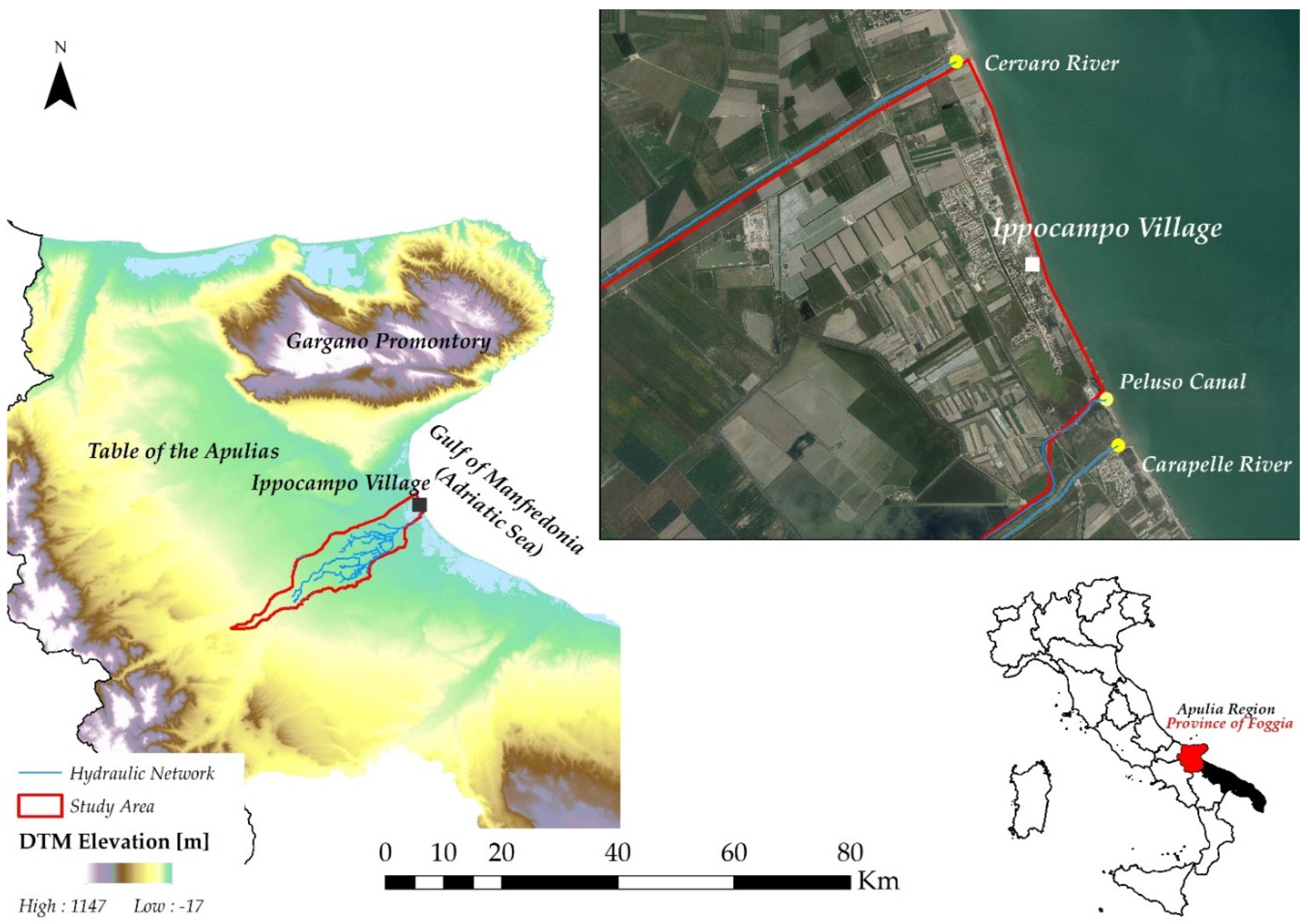
2. The Study Area
The examined area is located within the Gulf of Manfredonia in the Adriatic Sea (Apulia Region, Southern Italy) and the coastline is oriented north–south with a narrow sandy beach backed by salt marshes and cultivated crops.
The study area is crossed by an important hydrographic network and is bounded on the north by the Cervaro River, on the south by the Peluso canal and the Carapelle River, and on the east by the Adriatic Sea (as shown in Figure 1).
The rainfall regime is Mediterranean with an average rainfall of 442.1 mm per year and an average of 63.4 rainy days per year. The maximum rainfall occurs in the autumn–winter period, with a strong dryness during the summer months [42].
Elevation is lower than 15 m above mean sea level and the area also includes a large part of the ancient Salso Lake. This area has historically been mostly uninhabited and wild, being naturally rich in marshes and swamps, and it is classified as a SIC (Site of Community Importance for the European Commission Habitats Directive—92/43/EEC) [43] (SIC IT9110005 “Capitanata wetlands”).
Starting from the 1970s, some local landowners gave impetus to an extensive reclamation of the area, which had already begun since the early twentieth century, transforming a highly natural landscape into intensively cultivated agricultural land and built-up areas. A large network of reclamation channels, currently in a poor state of conservation, was specifically built. The expansion of the cultivated land, to produce vegetables close to the coastline, destroyed the coastal dune cordon reducing it to a narrow embankment to protect crops. In that period, the Villaggio Ippocampo tourist complex was also built and further developed in the following years and nowadays in the summer period, there are more than 15,000 residents.
Since the mid-20th century, the long sandy beaches of the Gulf of Manfredonia have suffered a significative shoreline retreat due to a massive anthropic action [44]. At present, the retreating coastline extends from Margherita di Savoia to the Ippocampo tourist village and the erosive process is progressing towards the port of Manfredonia [31]. Due to the hundreds of protection structures built in the past 40 years, the examined area has especially been observed in the last decades, becoming a “case study” [18].
In addition to coastal erosion issues, the study area is also aggravated by flooding hazard [35] because, due to the presence of low-lying and depressed areas, coastal flooding occurs also during ordinary storms. Furthermore, sea storms are often associated with significant meteoric events with consequent river overflow. However, it should be noted that, despite the twentieth-century anthropization, half of the territory to be examined can be classified as “natural area”. About 50% of the natural areas are listed as habitats indicated in the Habitats Directive 92/43/EEC [43].
Trying to analyze the land-use, it is evident that the area, as already mentioned, is characterized by a strong anthropization, which totally transformed, in the last decades, the natural environments. Specifically, the construction of the “Ippocampo” tourist complex took place on brackish moist soils characterized by halophilous vegetation, which was recognized by the European Community as a habitat of community importance. The phenomenon of anthropization has also affected the beaches and the entire dune system, both for the construction of the shores and the cultivation of the land. Together with the total obliteration of the dune cordon to make way for the bathing structures, various degrees of transformations of coastal dunes are found, ranging from the construction of an embankment to protect the internal spaces with the planting of exotic species (e.g., Carpobrotus acinaciformis), to the reduction of the original dune and its typical dune vegetation (e.g., Ammophila sp.). These data highlight the importance of the examined area from the point of view of environmental conservation.
3. Materials and Methods
3.1. Numerical Model Description
To assess the coastal inundation risk zones in the case study area along the Adriatic coast (Figure 1), two-dimensional hydraulic modeling software (FLO-2D software) has been used to simulate a storm surge approaching a low sandy beach added to river flooding.
The FLO-2D model [45] is generally used for different types of hydraulic tests such as the propagation of floods and debris flow events. It allows us to simulate flooding on a complex topography and a given roughness based on the conservation of volume. O’Brien [36] also simulated ocean storm surge scenarios occurring in Hawaii by mapping the inundation areas. To simulate inland flooding, FLO-2D requires the topography of the area, which can be represented by Digital Terrain Model (DTM) points, roughness coefficients, and input hydrographs. The FLO-2D model produces time step flow depth and velocity maps and the maximum flow depth map outlining the maximum area of inundation.
The entire calculation domain extends 65.5 km2 and consists of a square mesh grid with a resolution of 15 m. In the model, the rainfall input has been entered in the form of hydrograph (discharge versus time), whereas the storm surge has been treated as a boundary element with a stage–time relationship.
3.2. Rough Data Collection
The fundamental characteristics of the climate were derived by analyzing and processing the data for the fifty years 1951–2000 collected by the Hydrological Annals (Hydrographic Service of the Ministry of Public Works) [42], referring to the “Manfredonia” thermopluviometric station (2 m a.s.l.) a few kilometers from the study area.
The sea level analysis was carried out exploiting tidal data acquired from 2007 to 2015 by the tide station located in the port of Manfredonia belonging to Apulia Region Meteomarine Network (also known as SIMOP) [46]. That regional meteomarine network has been operating since 2006, collecting wave, wind, and tidal data along the Apulian coastline [47].
The Manfredonia tide station, in particular, was deployed because there was a lack of data exactly in an area at high risk for coastal flooding [21]. The tidal station is equipped with an ultrasonic gauge incorporating an internal temperature sensor to compensate for temperature changes. Identification of anomalous data, spikes, and timing errors has been carried out following quality control checks [48], and spurious records have been removed from the time series. The amplitude of tidal oscillations recorded in the Gulf of Manfredonia during the observation period is of the order of tens of centimeters and is compatible with sea level variations in the Mediterranean Sea.
The analysis of sea level data showed an increase in the mean sea level and an increase in tidal peaks starting from 2009, with a maximum recorded on 6 February 2015 equal to +0.70 m a.s.l. [31]. A sudden increase in mean sea level has been reported from winter 2008–2009, with a variation between 2007 and 2009 of about 10 cm, followed by a decrease in 2011, while no significant changes have been found in meteorological tides [49].
For the examined site, offshore observed wave data are not available, hence we referred to a wave time series collected about 130 km south of Ippocampo by a directional wave buoy moored offshore Monopoli in the Adriatic Sea belonging to the Italian National Buoy Network.
The observed wave dataset covers an 18-year period, from 1990–2007, and consists of significant wave height (Hm0), peak wave period (Tp), and mean wave direction (Dm).
Offshore depth information was taken from the nautical maps produced by the Italian Navy Hydrographic Office (IIM) and a specific field campaign was carried out using a single-beam echo sounder associated with a GPS/RTK positioning system. Collected data were used to create a detailed bathymetric map up to a depth of about −20 m (Figure 2).
A high-resolution Digital Terrain Model (DTM) generated from LiDAR data covers the area and it has been further improved by additional topographic data acquired during a field survey. LiDAR data were used to create a structured computational grid with a cell size of 15 m. The entire calculation domain extends 65.5 km2 and the grid resolution was chosen to reduce the computational cost.
Flow resistance or “roughness” is represented by Manning’s friction coefficient “n” (s/m1/3) and, for floodplains, it depends on the substrate and vegetation density [50,51]. The surface roughness, in each simulation, was assumed equal to the default value in the model (0.04 s/m1/3) for all cells inside the computational domain.
3.3. Hydrologic Modeling
Following a consolidated technical practice in the regional area, the VA.PI. Apulia method [52] provided the estimation of the precipitation input.
To this purpose, the intensity–duration–frequency curves of precipitation (IDF) were defined. Each IDF curve is associated with both a scenario and a hydrographic sub-catchment. The study considered four return periods (TR = 1 year, TR = 30 years, TR = 50 years, and TR = 100 years) corresponding to four different scenarios. To suitably define the floodplain, since the whole hydrographic network included in the study area is composed of several river branches, it was necessary to identify a hydrological input for each of them. For this purpose, the overall domain was divided into sub-catchments, each pertaining to a stretch of the hydrographic network.
A monomial exponential expression derived from two-parameter law described the rainfall IDF curves:
where im is the average intensity of the precipitation, a function of the duration of the rainfall event (t) and the return period (TR); a is a parameter depending on the return period (TR) and considered area; and n is a parameter depending on the considered area.
A regional analysis of the annual maximum rainfall intensity, performed with a probabilistic model based on the use of a Two Component Extreme Value (TCEV) Distribution [53], maximum likelihood estimator, and hierarchical estimation of regional model parameters [54], allowed the estimation of the rainfall IDF curves.
The regional analysis was based on the VA.PI. method, provided by the National Group for the Defense from Hydrogeological Disasters [52], through the probabilistic analysis of annual maximum rainfall of assigned duration (1, 3, 6, 12, and 24 h) [42].
The VA.PI. method is a national report, articulated through a series of “regional reports”, that presents a synthesis of the studies carried out in different areas of the national territory. Each regional report explains how to use the entire procedure developed at the local level.
The regional report for the Apulia Region defines an effective procedure [52]. Exactly, through a “regionalization” process, homogeneous zones for rainfall were identified within the territory of the Apulia Region. An equation was associated with each zone to evaluate the relative IDF curve, as a function of the rainfall depth (expressed in mm).
The whole area examined corresponds to the relationship:
where h represents the rainfall depth; t is the time of the precipitation storm; and z is the mean elevation of the basin. In this case, Zone 2 is not dependent on the parameter z.
Studies by Eagleson [55] and Penta [56] made it possible to apply the procedure to the basins of Southern Italy.
Moreover, the growth factor KT allowed pondering the IDF curve dependence from the return period (TR). Statistical studies suggest the growth factor is constant for the whole northern Apulia Region [52], individuated within the previously mentioned VA.PI. Apulian Regional Report.
In particular, for these zones, the VA.PI. report defines the following equation to rate the growth factor value:
For each duration of rainfall, values of corrected rainfall depth (hc) are estimated:
The following relationship couples the corrected rainfall depth (hc) with the mean intensity of rainfall:
Thus, the IDF curve can also be expressed, in terms of rainfall depth, as:
The IDF curves led to the determination of the peak flow rates of the basins hydrographs, which is an input of the flooding modeling through the runoff curve number method proposed by the USDA Soil Conservation Service Agency (SCS-CN) [57].
This method is based on the use of the empirical parameter called Curve Number (CN), widely used in hydrology to estimate the surface runoff from the mass rainfall. The CN parameter depends on the soil type, land use, treatment, and moisture condition [58], and it can vary between 0 and 100. Following the indications of the local basin authority contained in the PAI Puglia [35], in this case, all values of CN were referred to a wet condition of the soil (AMC-III), for the benefit of security.
For each sub-basin considered in the computational domain, floods with a semi-distributed model were estimated, based on the average height, slope, surface, length of mainstream, and CNIII values of the relative basin [59].
Table 1 reports the values of CN-III and the peak flow rate in m3/s for each sub-catchment.
The shape adopted for the hydrograph is triangular, with the discharge peak at the time of concentration (tc) of each sub-catchment.
The time of concentration (tc) parameter was estimated through the relationship:
and the Mockus formula, provided in [60], to evaluate the Lag Time (tl)
where L is the maximum flow length, expressed in kilometers; s is the mean slope; and CN is the value of the Curve Number parameter.
Fiorentino [61] conceived a method for estimating flood volumes based on the use of flood reduction curves, which led to the assessment of the hydrograph’s overall duration.
The so-called flood reduction curve expresses the relationships between the flood peaks and the volumes passing through. It represents the ratio between the index flow rate on the variable duration and the peak flow rate for a given return period (TR), described by the following relationship:
where is the coefficient of flood reduction, depending on the duration and the return period (TR); is the index flow rate, depending on the duration and the return period (TR); and is the peak flow rate, depending on the return period (TR).
Bacchi [62] explained that the dependence on the return period, under suitable hypotheses on the frequency distribution of the flows, can be neglected. Thus, the reduction curve can also be defined as the ratio between the average of the extremes of a given duration and the index peak flow rate .
Conceptual approaches have been developed to allow an application even in ungauged basins. Several authors have proposed formulas in which the various parameters of the reduction curve are directly related to the geomorphoclimatic characteristics of the basin, such as the basin lag time (tl) and the coefficient n, exponent of the two parameter IDF curve.
In 1985, Fiorentino [61] proposed a formulation of the reduction curve, based on the runoff model’s conceptual hypothesis of a linear reservoir:
It is a monoparameter formulation, in which the parameter k [63] is dependent on the lag time (tl) and the IDF exponent n:
Once the k value for each sub-catchment is established, the assessment of the flood volume ( is then possible using the following expression:
Replacing the expression of in Equation (12):
The overall duration of the input hydrograph has been established to obtain a flood volume (), for each return period considered, higher than that () calculated by maximizing the Equation (13).
3.4. Coastal Modeling
To investigate coastal flooding, the specific input data required for the FLO-2D model are water levels at the shoreline, as a function of time, calculated as the sum of storm surge, astronomical tide, wave set-up, and wave run-up.
Storm surge is defined as the sum of the effects that barometric pressure, wind stress, Coriolis force, and wave breaking have on sea level. The sea surface elevation recorded by tide gauges is the sum of astronomical and meteorological tide induced by wind, storms, and atmospheric pressure disturbances, which can be split up performing harmonic analysis [64,65]. The meteorological tide can be predicted by implementing the extremal analysis of tidal residuals to obtain events with a given return period.
The 1-, 30-, 50-, and 100-year return period storm surges were estimated in the Gulf of Manfredonia exploiting a hindcast tide dataset calculated using a numerical model Regional Ocean Modeling System (ROMS) [31].
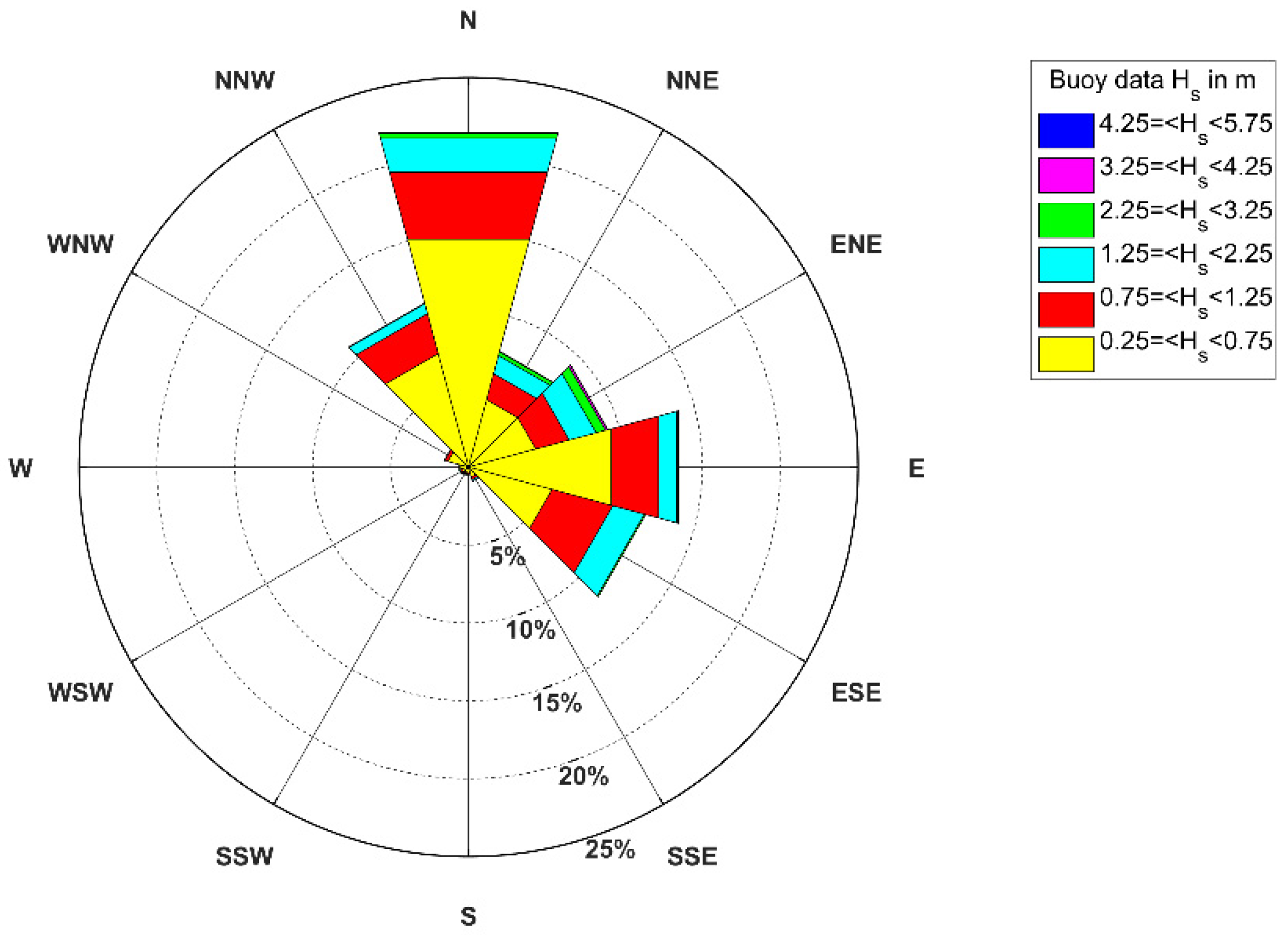
To investigate wave-induced sea level set-up, the available wave dataset observed offshore Monopoli was transferred offshore Ippocampo by using the geographical transposition of wave gauge data [66] based on the empirical Sverdrup–Munk–Bretschneider (SMB) model [67]. Estimated wave data were analyzed and the distribution of percentage frequency of wave direction and height was analyzed. Wave climate offshore in the Gulf of Manfredonia is moderate and the highest sea storms approach from ENE (Figure 3).
In addition, the extremal wave analysis was carried out fitting all the waves coming from homogeneous sectors [68] above a threshold value (peak over threshold method [69]) to a Weibull extreme-value distribution (Table 2).
Extremal waves were propagated towards the coast using the Simulating WAves Nearshore (SWAN) model [70,71] using a nesting approach to improve the resolution in the coastal area. A high-resolution 10-m grid, extending from shoreline to −10 m contour, was nested in a coarse grid (at 200-m resolution) covering a large area in the Gulf of Manfredonia.
The SWAN model was run to estimate wave heights and breaker depths using the values of 1-, 30-, 50-, and 100-year return period waves.
Given the breaking wave characteristics, it is possible to evaluate wave run-up, defined as the maximum vertical extent of wave uprush on a beach or structure above the still water level (SWL).
Several formulas for predicting wave run-up have been developed from experimental studies [72,73,74,75]; in this work, the Stockdon formula was used [76]:
where Ru2% is the run-up level exceeded by two per cent of the incoming waves, H0 is offshore wave height, L0 is the offshore wavelength, and bf is the foreshore slope. The beach slope was evaluated by considering the mean slope of the vertical region whose height is two times the breaking depth [16]. As shown in Figure 2, a very slight slope (about 0.3%) can be detected along the sea bottom in the examined area.
The Stockdon equation already includes wave setup and requires offshore wave characteristics, thus the use of this formula is very convenient for cases of application to large areas and where bathymetric data are not available.
3.5. Risk Assessment
Generally, for natural calamitous events (landslides, floods, etc.), the risk can be quantified as the product of hazard, vulnerability, and exposure [78]. Hazard represents the probability of occurrence of a specific hazard scenario with a given return period. Vulnerability is the degree of damage of the elements at risk resulting from the occurrence of a natural hazard of a given intensity [79]. Finally, exposure defines the system at risk (its components, elements, functions, activities, etc.) and its value (social, economic, functional, etc.).
The quantitative assessment of risk, in monetary terms, was carried out by computing the economic losses consequent to potential flood events for different return periods (1, 30, 50 and 100 years). Firstly, all elements at risk were recognized and typologically classified in the study area. In total, 20 types of exposed assets were identified: electric cabin, aqueduct cabin, swimming pool, sports area, cistern, shed, agricultural shed, building, tree planted area, arable crop, unqualified garden, nude soil, shrub pasture, Mediterranean shrub area, olive grove, orchard, vineyard, greenhouse, urban road, and extra-urban road. These elements at risk were subsequently grouped into five categories, namely buildings, other structures, infrastructures, specialized land use, and unspecialized land use, which are characterized by different damage functions.
Among the elements at risk, the population was not considered for different reasons. First, it represents an intangible loss [80]. Moreover, assessing the temporal and spatial distribution of people in an area is an objectively difficult goal and quantifying the economic value associated with injuries or deaths is a complex ethical task. Population is a mobile asset [81] and, for this reason, the evaluation of exposure of persons would require the calculation of the conditional probability of persons being present in buildings or on the roads at the occurrence time of natural hazards [78].
The procedure used for evaluating quantitatively both the exposure of elements at risk and the economic risk was derived from [38,39]. The exposure assessment was carried out by overlaying of the elements with each flooding hazard map and evaluating the amount of assets in each flooding areas and quantifying the economic values for the various flood hazard scenarios (Figure 4, Figure 5 and Figure 6). Each type of element at risk was quantified in terms of areal extent (square meters or hectares). The spatial distribution of assets was combined individually with the four flooding hazard maps to obtain the number of elements potentially affected by flooding with 1-, 30-, 50-, and 100-year return period.
The spatial distribution of elements at risk was derived from the Regional Technical Map of Apulia at 1:5000 scale, for structures and infrastructures, and from Land Use Map of Apulia at 1:5000 scale, for land use categories, both available at geo-portal of Apulia Region [82].
Therefore, to evaluate the economic exposure associated with the different flooding hazard levels, unit market values or unit construction costs were assumed for each element at risk category. Starting from buildings, the unit market value (Euros per square meter) relative to 2019 was obtained from the Observatory of Real Estate Market (OMI) instituted by the National Territorial Agency. OMI is a cadastral database and provides maximum and minimum values for different kinds of buildings, such as residential, commercial, agricultural, etc., and for different zones of the inhabited area, e.g., center, suburbs, etc. In the area occupied from the village, residential, mainly villas, and commercial buildings are present. To obtain an overall unit economic value, a weighted mean among the market values related to residential and commercial buildings was calculated. The weights were derived considering the percentage distribution of commercial and residential buildings (about 30% and 70%, respectively). For sports areas, electric cabin, aqueduct cabin, agricultural sheds, cisterns, and swimming pools, the unit construction costs (Euros per square meter or cubic meter) were calculated from values defined in 1988–1989 by the National Territorial Agency. These values were updated, by calculating the inflation rate using data of ISTAT (National Institute of Statistics). In addition, the unit agricultural values (Euros per hectare) were obtained from the National Territorial Agency. The most recent data for the study area (included in the Foggia Province) are related to 2012. Finally, for roads, unit maintenance costs obtained from the Regional Price List of Apulia for 2019 were used. This unit maintenance cost includes mainly cleaning road work, i.e., mud removal from the roadway, drainage ditches, inspection wells, and scarps.
The quantitative evaluation of risk associated with the four flood hazard scenarios, in terms of economic expected losses, was carried out starting from the exposure estimation, according to Figure 7 and Figure 8. In particular, the exposed values associated to each flooding scenario were quantified by computing the amount of elements at risk (square meters, cubic meters, and hectares) involved in each flooding scenario and, subsequently, multiplying the amount of the individual exposed assets with their unit economic value.
For each category of elements at flood risk, the potential damages were obtained by taking into account their vulnerability to flood damages, expressed by flood-damage functions. Velocity and flood depth values, resulting from the hydraulic modeling and varying for each flood hazard scenario, permitted calculating a vulnerability (Ve) value, ranging from 0 to 1 (Table 3). Therefore, Ve defines the percentage of damages of economic assets in function of physical characteristics of floodwaters. In fact, each category of the five above-mentioned was associated with a different vulnerability flood-damage function. The flood damage functions of buildings, other structures, specialized, and unspecialized land use were referred to [40], whereas that of infrastructures was referred to [41].
The consequences were assessed by multiplying the exposed economic value of assets by the Ve values of each category of elements at risk. For each flooding scenario, the total consequences (or expected losses) were calculated by summing the values related to the five categories of elements at risk. The economic losses values associated with each flooding scenario were multiplied with the corresponding exceedance probability of hazard scenarios to obtain the related risk in monetary terms.
4. Results and Discussion
The first set of simulations was run to check the reliability of the inundated areas and the accuracy of the simulated flooded areas had been checked by comparing the model outputs with the effects of an observed event.
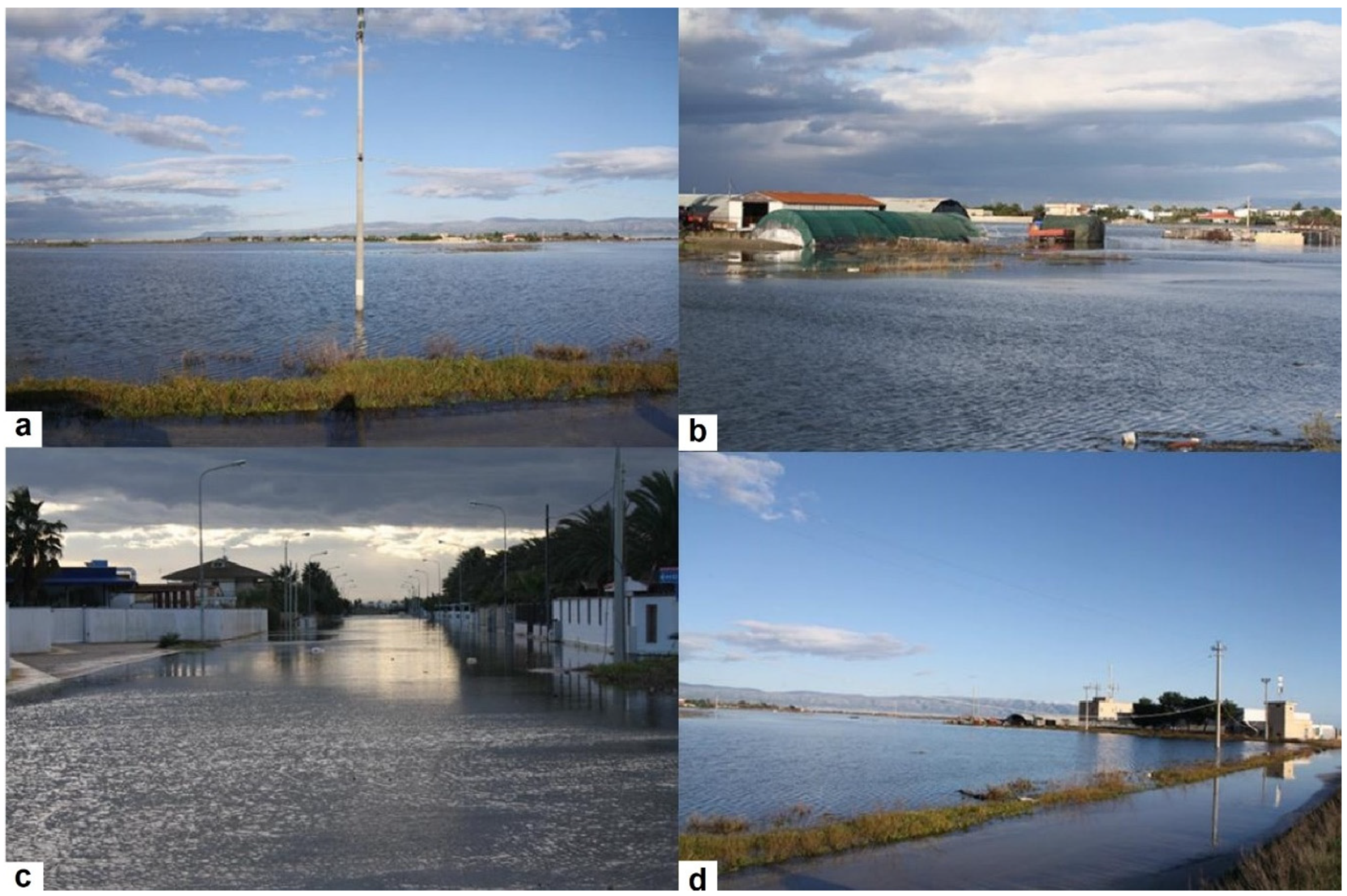
In November 2009, a severe meteo-marine event struck the examined area, causing flooding and considerable damages. In the hours following the disaster, a quick field survey was carried out in the area to detect inundated regions and numerous photographs had been taken (Figure 5). Initially, following the common practices for the evaluation of the risk on the coastal areas [21,22,23], a FLO-2D model based only on storm surge input was defined exploiting the water levels and wave data collected in the area. However, it proved unable to fully return the observed floodplain, because only the areas closest to the coast were flooded.
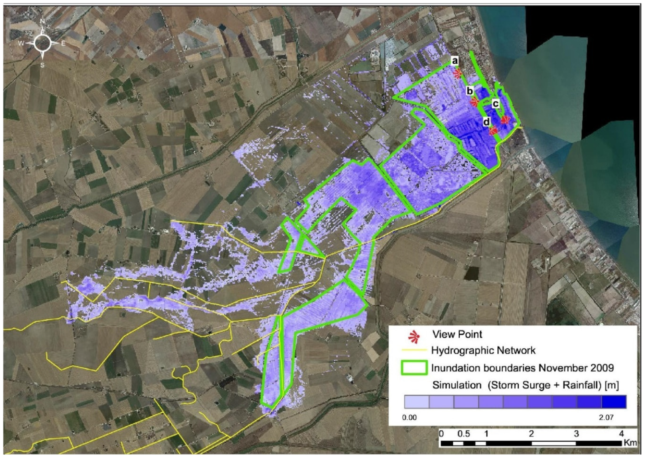
Therefore, a combined model that included both storm surge and flood input was run and the accuracy of the simulated inundation areas was tested comparing the model results with the observed flooded areas. Quite good accordance was found, as shown in Figure 6, even if some differences, especially in the agricultural area, can be explained considering that observed inundation boundaries have been collected during an expeditious survey along the damaged roads in the days following the event. In the urban zone, where the post-event flooding area was detected with extreme detail, the numerical results perfectly overlap.
After the model results validation, the FLO-2D [45] model processed for each selected scenario (TR = 1-, 30-, 50-, and 100-year return period) two flooding simulations, one considering only the storm surge contribution and one using the storm surge combined with the rainfall.
Storm surge and rainfall depth were modeled considering the same return period, since in the case of a small catchment, mostly located in the coastal areas, the same synoptic weather system may induce extreme sea level and heavy rainfall [83]. Moreover, Bevacqua et al. [84] and Moftakhari et al. [85] confirmed a substantial decrease in return periods if the joint occurrence probability of sea water level and river discharge is considered. Hence, in these cases, in favor of safety, it could be appropriate to consider the probability distribution of the extreme events of the two random variables substantially coincident, because the meteorological forcing is the same. Therefore, the presented combined model represents the worst-case scenario and could be a useful tool for coastal area management.
The simulation provided results in the form of flood maps in terms of flow depth and velocity. These maps presented zones affected by values of both flow depth and velocity that were negligible for the realistic evaluation of the connected hazard distribution. Technical literature called these areas “marginals”. The delimitation of the “marginal inundation areas” was carried out following the methodology suggested by the River Tevere Basin Authority [86].
The applied methodology conservatively considers a water depth above 0.2 m and a velocity flow greater than 0.3 m/s as the limits of danger, whereas the flooded areas with smaller values are defined as marginal areas. In particular, all water depth values >0.2 m were considered to identify flooding areas, regardless of velocity values. At the same time, all velocity values >0.3 m/s were considered, regardless of depth values.
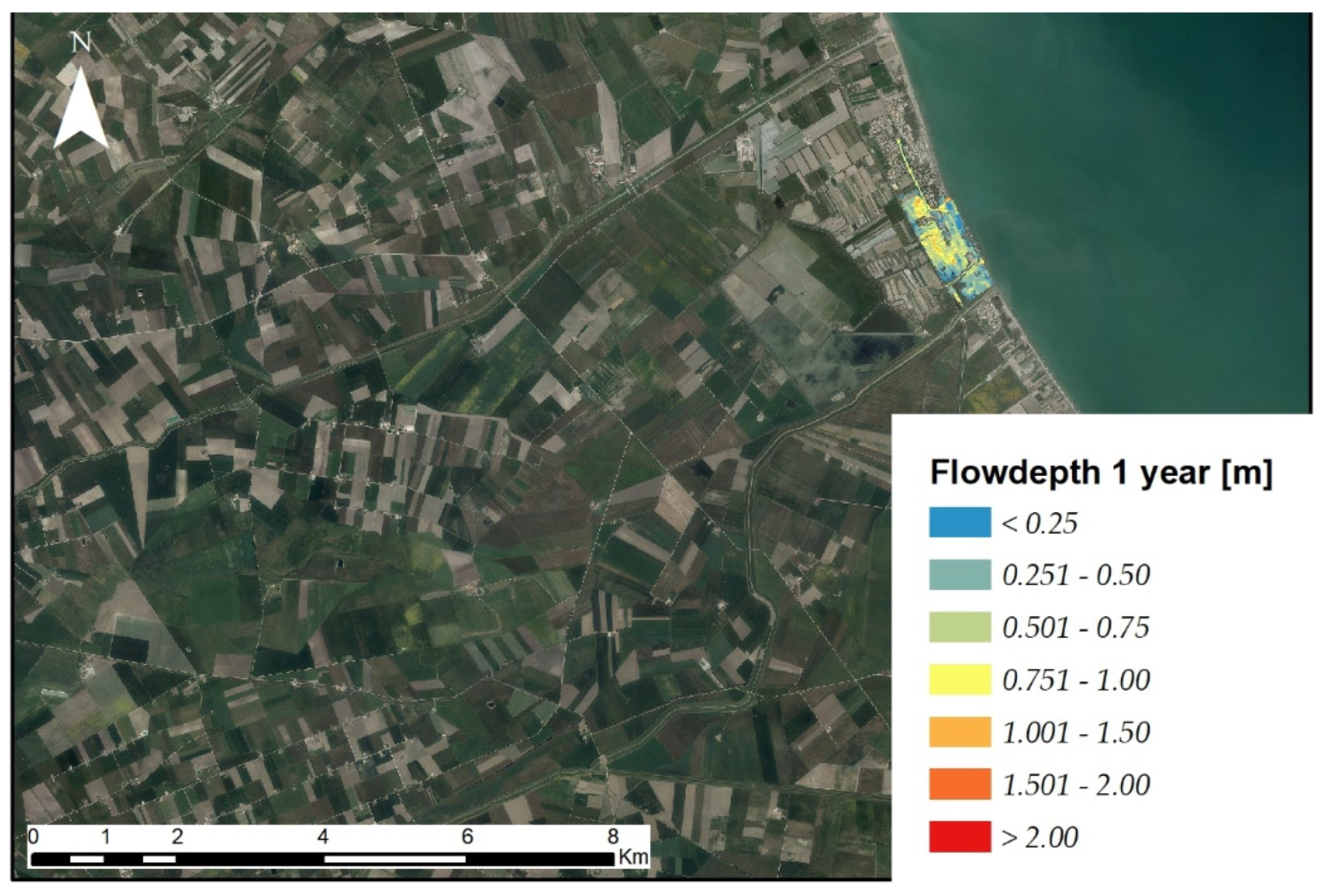
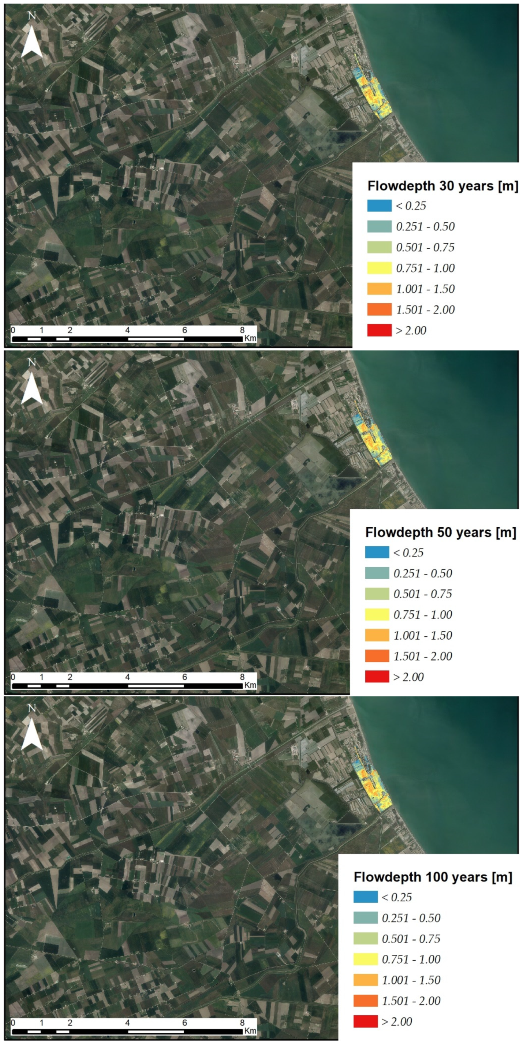
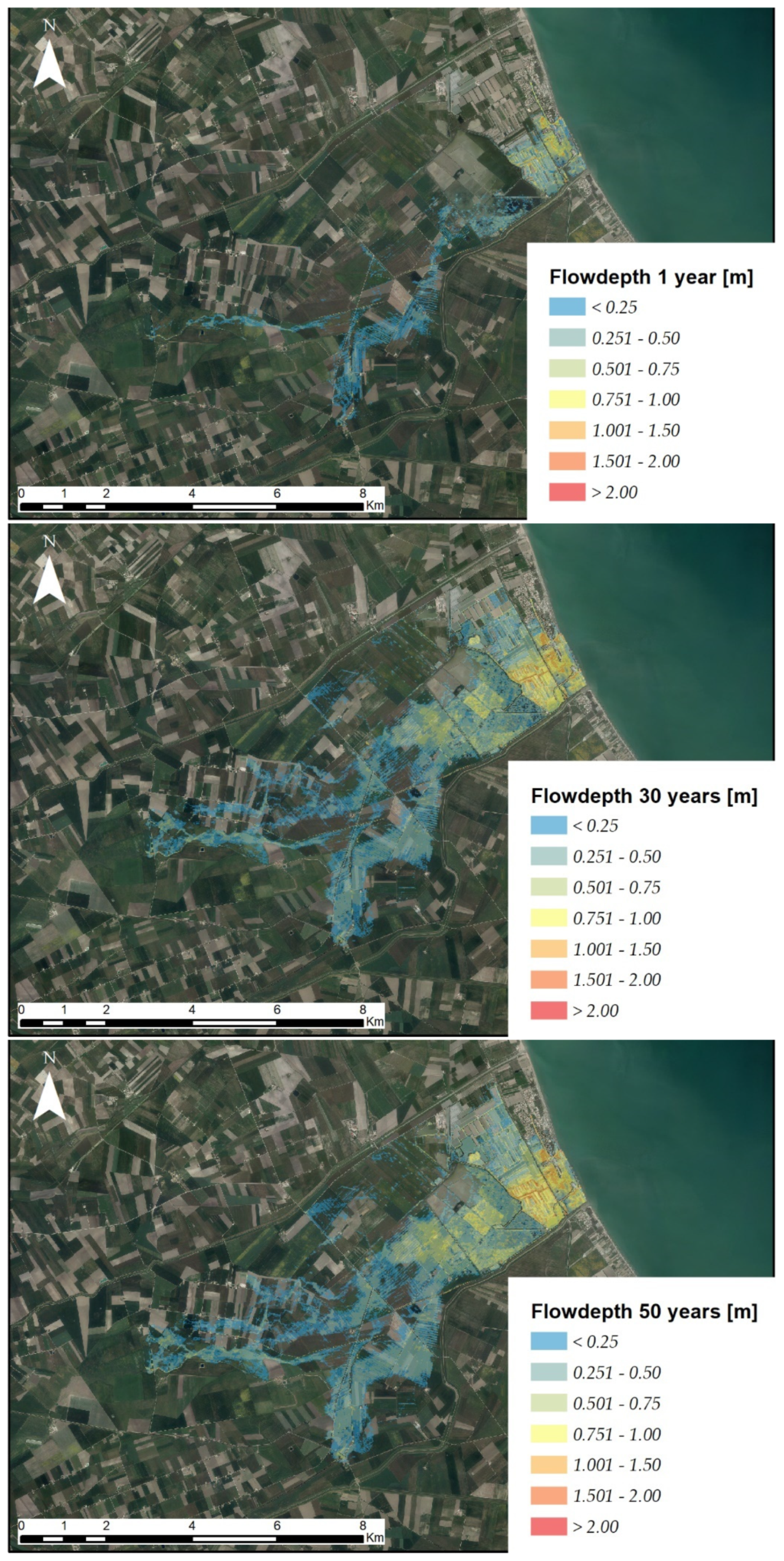
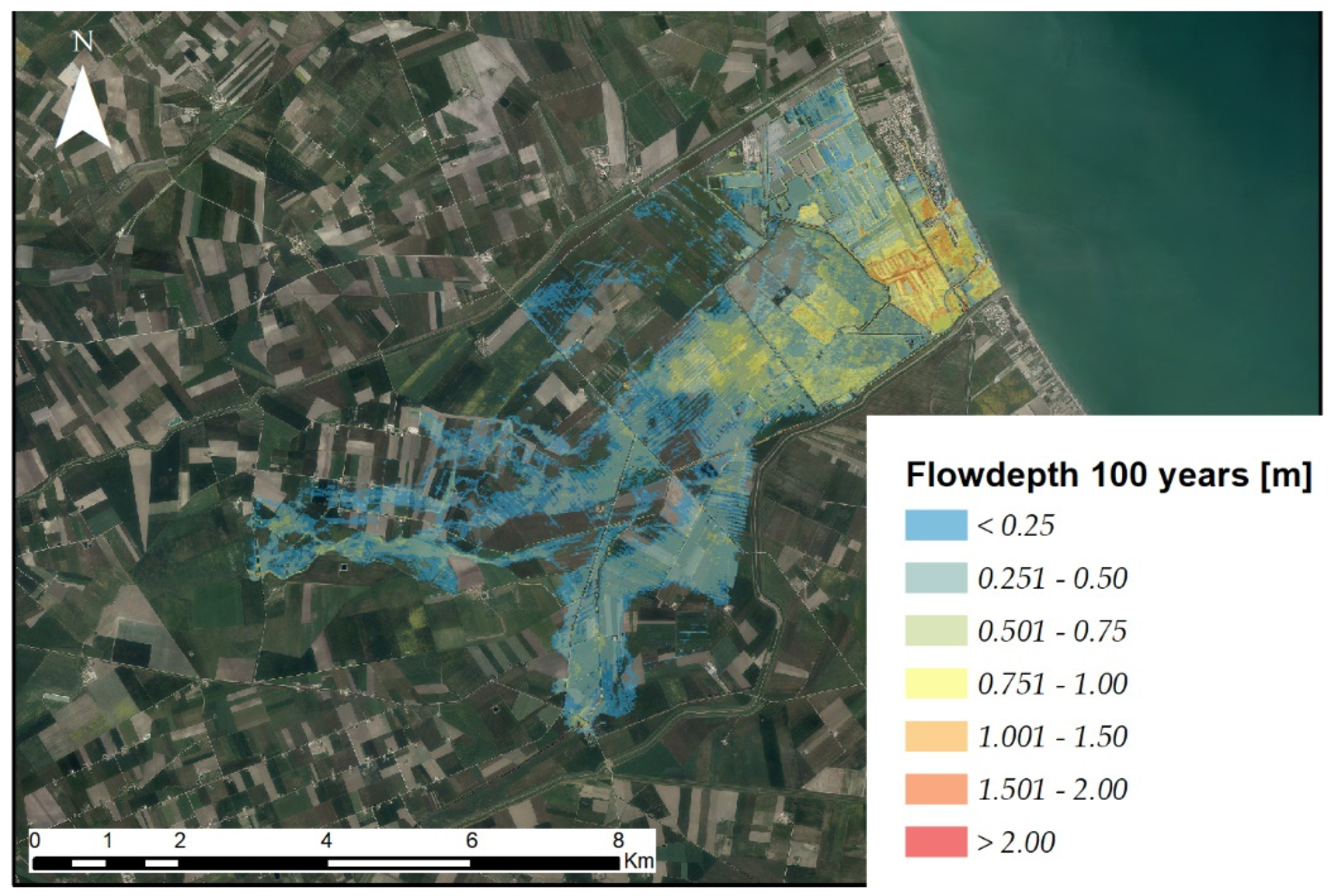
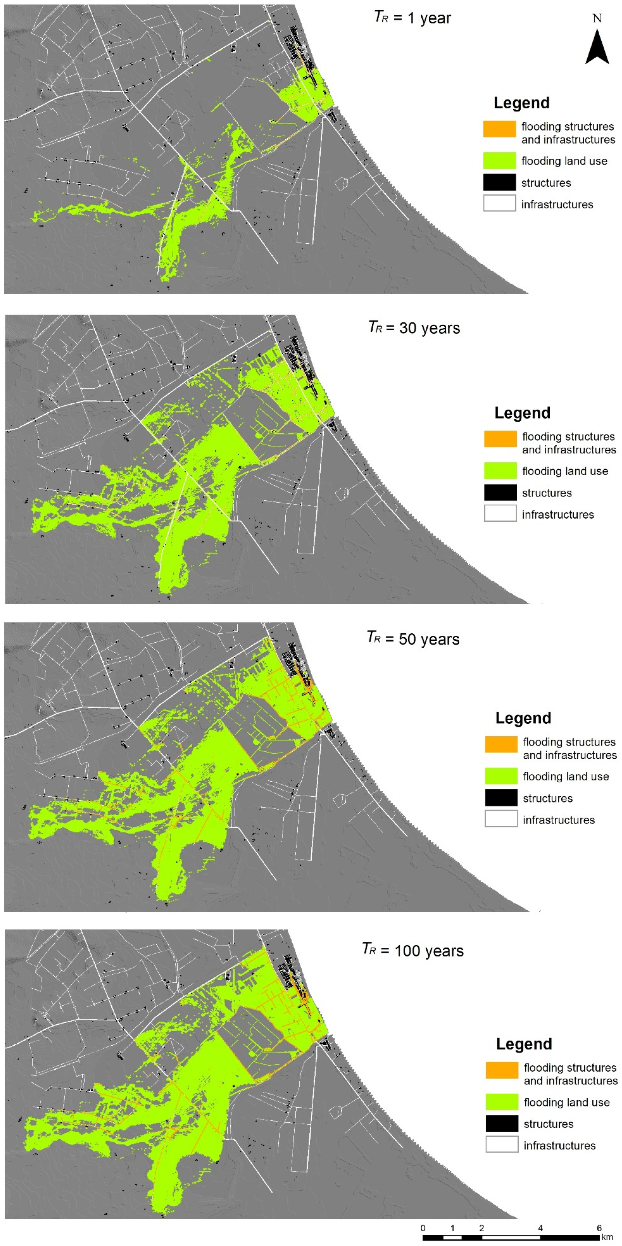
Following this approach, all flooded areas resulting from the hydraulic simulations were mapped (see Figure 7 for the storm surge model and Figure 8 for the integrated model). To develop hydraulic modeling, FLO-2D is preferred, for which the numerical stability was preliminarily verified. This aspect made possible simultaneously modeling both the storm surge input and the flood hydrographs for the different return periods, in a more detailed calculation domain. The inundation contours simulated with the FLO-2D model (see Figure 8) highlight the presence of large areas at risk of marine ingression in all the investigated scenarios and the flooded areas increase further if the rainfall is included in the model.
The zone most affected by flooding includes built-up areas, wetlands, and agricultural land, constituting a potential hazard for people, facilities, and viability. The presence of channels and rivers heavily affects the result of the analysis. The water channels, in fact, constitute a preferential way of marine ingression directing water inland for hundreds of meters and in the case of combining with heavy rain, due to the increased water depth in the channel, the flooding event involves a greater area. The extension of flooded areas increases as the year return period increases, but it is important to highlight that even a one-year return period event will inundate the urban area. Consequently, this scenario was also considered in the risk assessment of the study area.
The output of flooding simulations, in terms of flooding hazard maps, was combined with the distribution in the study area of elements at risk to carry out the exposure analysis according to Figure 4. This procedure was applied for both flooding simulations, i.e., both considering only the storm surge contribution and using the storm surge combined with the rainfall (combined model). In Figure 9, the elements at risk, subdivided into structures, infrastructures, and land use, involved in flooding areas derived from the four combined models are highlighted.
Subsequently, for each of flooding scenarios and each category of elements at risk, the amount of exposed assets potentially involved in the flooding events and their economic values were computed. Therefore, the consequences were obtained by multiplying the economic values of the exposed assets with vulnerability values, deduced from the damage functions in Table 3. Finally, the total economic losses associated with each flooding scenario were computed by summing the consequence values of the five categories of elements at risk. The results of exposure and risk assessment are synthesized in Table 4 and Table 5. The first one is related to modeling with only storm surge input, while the second one refers to the combined model (storm surge and rainfalls). The final values of risk, or economic losses, corresponding to a different return period of flooding events are also shown in Figure 10 in the form of risk curves.
Table 4 and Table 5 show that economic losses corresponding to the first scenario, flooding at one-year return period, are already relevant if compared with the other three scenarios. Therefore, it represents the risk scenario to be considered to plan mitigation measures. Moreover, the amount, in square meters, of structures (buildings and other structures) undergoes slight variations among the last three scenarios (TR = 30, 50 and 100 years). This is due to the configuration of flooding areas, which, as shown in Figure 9, are nearly similar for these scenarios. This effect is even more evident for the storm surge modeling (in Table 4), observing the values of total economic losses for 30-, 50-, and 100-year scenarios. Land elevation in coastal areas subject to inundation from storm surge is below mean sea level and, hence, a low return period event is sufficient to completely flood the urban area.
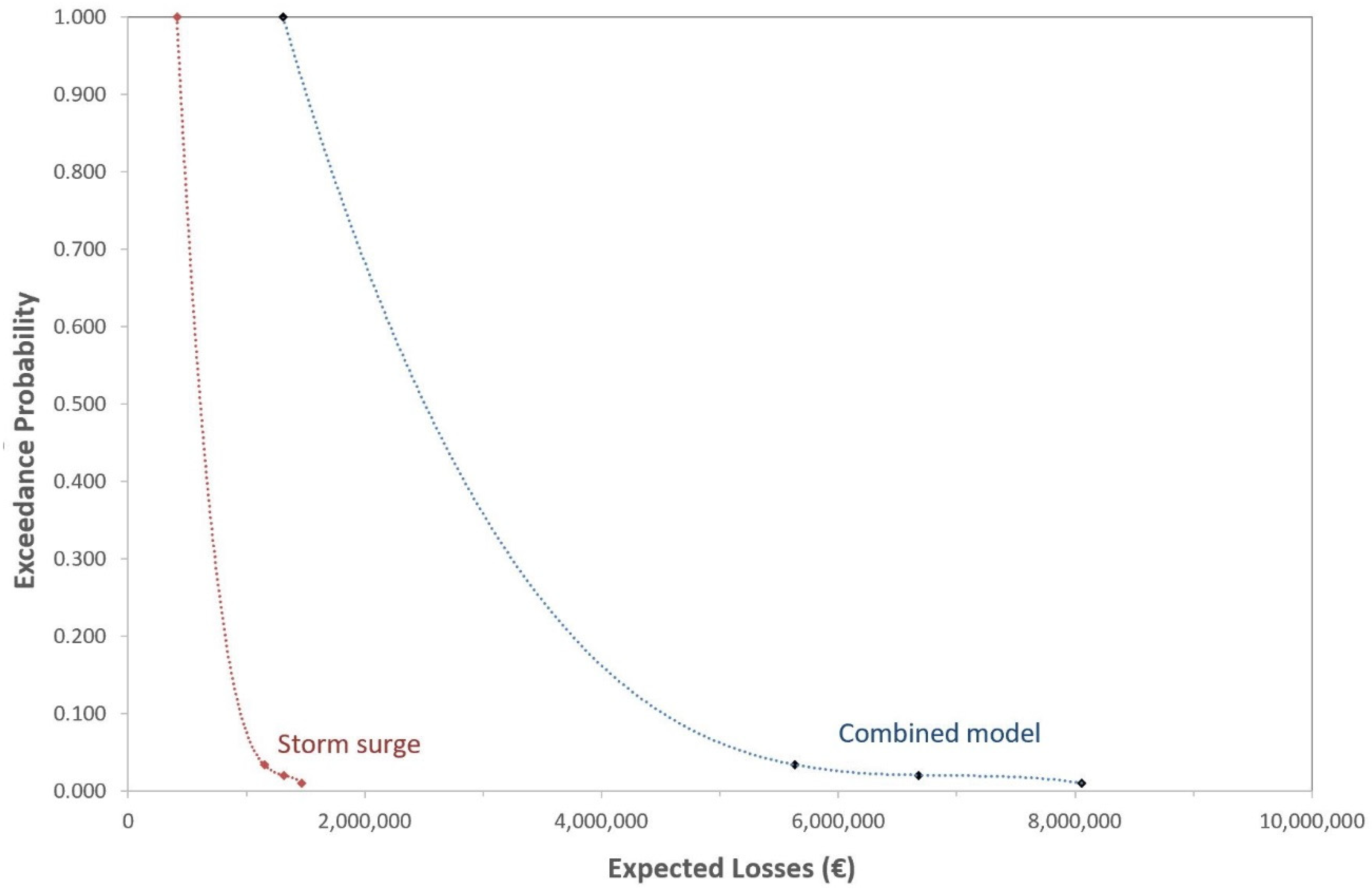
Furthermore, the elements at risk mostly affected by flooding events are agricultural areas and roads, which represent preferential flow paths. Finally, the risk curves in Figure 10 highlight that the combined flood modeling provides more complete results in terms of potential economic losses. This aspect is confirmed in Figure 7, which shows that the storm surge alone could not sufficiently justify the flooding areas.
5. Conclusions
Quantitative risk estimation methods are often limited by the lack of data on calamitous events, information on damages, and related costs, although an increase availability of data is lately being recorded in the technical literature with regard to risk related to natural hazards.
In this paper, a “combined hydraulic modeling” is proposed to identify the hazard map in an ungauged coastal area. In contrast with most studies, in which the risk assessment in a coastal area only takes into account the storm surge contribution in adherence to the classical approach, this study shows that in low lying areas with presence of water channels the classical approach would lead to an underestimation of the economic risk. To improve the estimate of the economic risk, a two-dimensional hydraulic model was adopted to assess the coastal inundation risk zones in the area along the Adriatic coast. The model enabled the simulation of a storm surge approaching a low sandy beach simultaneously affected by river flooding.
Firstly, the output of the model was validated by employing real data to demonstrate its effectiveness in identifying coastal areas exposed to storm surge inundation.
Secondly, the output of flooding simulations was combined with the distribution of the elements at risk in the study area to determine the level of exposure. This procedure was applied for both flooding simulations, i.e., in the presence of only storm surge contribution and in combination with rainfall. Subsequently, the amount of exposed assets potentially involved in the flooding events and the related economic values were computed for each flooding scenarios and for each category of elements at risk.
Finally, the total economic losses associated with each flooding scenario were computed by summing the consequence values of all categories of elements at risk.
The results show that economic losses corresponding to the first scenario analyzed are already relevant when compared with the other three scenarios for floods of one-year return period. These results represent the risk scenario to be considered to plan mitigation measures. The results also show the surface area amount, in square meters, of civil structures subject to slight variations in the last three scenarios considered with return periods of 30, 50, and 100 years. This becomes even more evident for storm surge modeling when observing the values of total economic losses for the 30-, 50-, and 100-year return period scenarios. The particular trend of the risk curves determined can be explained by the peculiar topography of the flooded area are characterized by negative elevation respect to the medium sea level. This is the reason a low return period event can also be sufficient to completely flood the urban area.
The risk curves for the flood combined modeling provide more complete results in terms of potential economic losses. This was confirmed by the necessity of the combined hydraulic model which is proposed in present work.
The approach adopted in this work can deliver a concrete support to decision-makers responsible for the identification of measures aimed at reducing the flood risk and for the implementation of flooding protection policies detailing safety interventions. A further development of this work will account for the indirect and intangible losses at basin scale in accordance with the 2007/60 Flood Directive.
Author Contributions
C.A., M.F.B., and M.G.M. conceived the work. C.A. and G.I. performed hydrologic and hydraulic modeling. M.F.B. and M.G.M. performed coastal modeling. R.P. performed risk analysis. All authors analyzed the results. M.F.B., R.P., and C.A. drafted and revised the manuscript. All authors have read and agreed to the published version of the manuscript.
Funding
This research received no external funding.
Acknowledgments
The authors gratefully acknowledge the support received for English editing by CEng MICE Martino Abbattista.
Conflicts of Interest
The authors declare no conflict of interest.
References
- Recanatesi, F.; Petroselli, A.; Ripa, M.N.; Leone, A. Assessment of stormwater runoff management practices and BMPs under soil sealing: A study case in a peri-urban watershed of the metropolitan area of Rome (Italy). J. Environ. Manag. 2017, 201, 6–18. [Google Scholar] [CrossRef]
- Apollonio, C.; Balacco, G.; Novelli, A.; Tarantino, E.; Piccinni, A.F. Land Use Change Impact on Flooding Areas: The Case Study of Cervaro Basin (Italy). Sustainability 2016, 8, 996. [Google Scholar] [CrossRef] [Green Version]
- Blöschl, G.; Ardoin-Bardin, S.; Bonell, M.; Dorninger, M.; Goodrich, D.; Gutknecht, D.; Matamoros, D.; Merz, B.; Shand, P.; Szolgay, J. At what scales do climate variability and land cover change impact on flooding and low flows? Hydrol. Process. 2007, 21, 1241–1247. [Google Scholar] [CrossRef]
- Novelli, A.; Tarantino, E.; Caradonna, G.; Apollonio, C.; Balacco, G.; Piccinni, F. Improving the ANN Classification Accuracy of Landsat Data Through Spectral Indices and Linear Transformations (PCA and TCT) Aimed at LU/LC Monitoring of a River Basin. In Proceedings of the 16th International Conference on Computational Science and Its Applications, Beijing, China, 4–7 July 2016. [Google Scholar]
- Nardi, F.; Vivoni, E.R.; Grimaldi, S. Investigating a floodplain scaling relation using a hydrogeomorphic delineation method. Water Resour. Res. 2006, 42, W09409. [Google Scholar] [CrossRef]
- Hill, A.R. Stream chemistry and riparian zones. In Streams and Ground Waters; Jones, J., Mulholland, P., Eds.; Elsevier: New York, NY, USA, 1999; pp. 83–110. [Google Scholar]
- Katsuyama, M.; Ohte, N.; Kabeya, N. Effects of bedrock permeability on hillslope and riparian groundwater dynamics in a weathered granite catchment. Water Resour. Res. 2005, 41, W01010. [Google Scholar] [CrossRef]
- Vivoni, E.R.; Entekhabi, D.; Bras, R.L.; Ivanov, V.Y.; Van Horne, M.P.; Grassotti, C.; Hoffman, R.N. Extending the Predictability of Hydrometeorological Flood Events Using Radar Rainfall Nowcasting. J. Hydrometeorol. 2006, 7, 660–677. [Google Scholar] [CrossRef]
- Townsend, P.A. Relationships between vegetation patterns and hydroperiod on the Roanoke River floodplain, North Carolina. Plant Ecol. 2001, 156, 43–58. [Google Scholar] [CrossRef]
- Jung, M.; Burt, T.P.; Bates, P.D. Toward a conceptual model of floodplain water table response. Water Resour. Res. 2004, 40, W12409. [Google Scholar] [CrossRef]
- Williams, W.A.; Jensen, M.E.; Winne, J.C.; Redmond, R.L. An automated technique for delineating and characterizing valley-bottom settings. Environ. Monit. 2000, 64, 105–114. [Google Scholar] [CrossRef]
- Petroselli, A.; Grimaldi, S. Design hydrograph estimation in small and fully ungauged basins: A preliminary assessment of EBA4SUB framework. J. Flood Risk Manag. 2018, 11, S197–S210. [Google Scholar] [CrossRef]
- Grimaldi, S.; Petroselli, A. Do we still need the Rational Formula? An alternative empirical procedure for peak discharge estimation in small and ungauged basins. Hydrol. Sci. J. 2015, 60, 67–77. [Google Scholar] [CrossRef]
- Młyński, D.; Petroselli, A.; Walega, A. Flood frequency analysis by an event-based rainfall-runoff model in selected catchments of southern Poland. Soil Water Res. 2018, 13, 170–176. [Google Scholar]
- Neumann, B.; Vafeidis, A.T.; Zimmermann, J.; Nicholls, R.J. Future Coastal Population Growth and Exposure to Sea-Level Rise and Coastal Flooding—A Global Assessment. PLoS ONE 2015, 10, e0118571. [Google Scholar] [CrossRef] [PubMed]
- Di Risio, M.; Bruschi, A.; Lisi, I.; Pesarino, V.; Pasquali, D. Comparative Analysis of Coastal Flooding Vulnerability and Hazard Assessment at National Scale. J. Mar. Sci. Eng. 2017, 5, 51. [Google Scholar] [CrossRef] [Green Version]
- Bruno, M.F.; Molfetta, M.G.; Pratola, L.; Mossa, M.; Nutricato, R.; Morea, A.; Nitti, D.O.; Chiaradia, M.T. A Combined Approach of Field Data and Earth Observation for Coastal Risk Assessment. Sensors 2019, 19, 1399. [Google Scholar] [CrossRef] [Green Version]
- Archetti, R.; Damiani, L.; Bianchini, A.; Romagnoli, C.; Abbiati, M.; Addona, F.; Airoldi, L.; Cantelli, L.; Gaeta, M.G.; Molfetta, M.G.; et al. Innovative strategies, monitoring and analysis of the coastal erosion risk: The STIMARE project. In Proceedings of the 29th International Ocean and Polar Engineering Conference, Honolulu, HI, USA, 16–21 June 2019. [Google Scholar]
- Bates, P.D.; Dawson, R.J.; Hall, J.W.; Horritt, M.S.; Nicholls, R.J.; Wicks, J.; Hassan, M.A. Simplified two-dimensional numerical modelling of coastal flooding and example applications. Coast. Eng. 2005, 52, 793–810. [Google Scholar] [CrossRef]
- Postacchini, M.; Lalli, F.; Memmola, F.; Bruschi, A.; Bellafiore, D.; Lisi, I.; Zitti, G.; Brocchini, M. A model chain approach for coastal inundation: Application to the bay of Alghero. Estuar. Coast. Shelf Sci. 2019, 219, 56–70. [Google Scholar] [CrossRef]
- Krestenitis, Y.N.; Androulidakis, Y.S.; Kontos, Y.N.; Georgakopoulos, G. Coastal inundation in the north-eastern mediterranean coastal zone due to storm surge events. J. Coast. Conserv 2011, 15, 353–368. [Google Scholar] [CrossRef]
- Martinelli, L.; Zanuttigh, B.; Corbau, B. Assessment of coastal flooding hazard along the Emilia Romagna littoral. Coast. Eng. 2010, 57, 1042–1058. [Google Scholar] [CrossRef]
- Perini, L.; Calabrese, L.; Salerno, G.; Ciavola, P.; Armaroli, C. Evaluation of coastal vulnerability to flooding: Comparison of two different methodologies adopted by the Emilia-Romagna region (Italy). Nat. Hazards Earth Syst. Sci. 2016, 16, 18. [Google Scholar] [CrossRef] [Green Version]
- Teng, J.; Jakeman, A.; Vaze, J.; Croke, B.F.; Dutta, D.; Kim, S. Flood inundation modelling: A review of methods, recent advances and uncertainty analysis. Environ. Model. Softw. 2017, 90, 201–216. [Google Scholar] [CrossRef]
- Tang, H.S.; Steven, I.; Chien, J.; Temimi, M.; Blain, C.A.; Ke, Q.; Kraatz, S. Vulnerability of population and transportation infrastructure at the east bank of Delaware Bay due to coastal flooding in sea-level rise conditions. Nat. Hazards 2013, 69, 141–163. [Google Scholar] [CrossRef]
- Joyce, J.; Chang, N.B.; Harji, R.; Ruppert, T.; Singhofen, P. Cascade impact of hurricane movement, storm tidal surge, sea level rise and precipitation variability on flood assessment in a coastal urban watershed. Clim. Dyn. 2018, 51, 383–409. [Google Scholar] [CrossRef]
- Ray, T.; Stepinski, E.; Sebastian, A.; Bedient, P.B. Dynamic Modeling of Storm Surge and Inland Flooding in a Texas Coastal Floodplain. J. Hydraul. Eng. 2011, 137, 1103–1110. [Google Scholar] [CrossRef]
- Torres, J.M.; Bass, B.; Irza, N.; Fang, Z.; Proft, J.; Dawson, C.; Kiani, M.; Bedient, P. Characterizing the hydraulic interactions of hurricane storm surge and rainfall–runoff for the Houston–Galveston region. Coast. Eng. 2015, 106, 7–19. [Google Scholar] [CrossRef] [Green Version]
- Ulbrich, U.; Lionello, P.; Belusic, D.; Jacobeit, J.; Knippertz, P.; Kuglitsch, F.G.; Leckebusch, G.C.; Luterbacher, J.; Maugeri, M.; Maheras, P.; et al. iClimate of the Mediterranean: Synoptic patterns, temperature, precipitation, winds and their extremes. In Climate of the Mediterranean Region—From the Past to the Future; Elsevier: Sydney, NSW, Australia, 2012; pp. 301–346. [Google Scholar]
- Cramer, W.; Guiot, J.; Fader, M.; Garrabou, J.; Gattuso, J.-P.; Iglesias, A.; Lange, M.A.; Lionello, P.; Llasat, M.C.; Paz, S.; et al. Climate change and interconnected risks to sustainable development in the Mediterranean. Nat. Clim. Chang. 2018, 8, 972–980. [Google Scholar] [CrossRef] [Green Version]
- Pasquali, D.; Bruno, M.; Celli, D.; Damiani, L.; Di Risio, M. A simplified hindcast method for the estimation of extreme storm surge events in semi-enclosed basins. Appl. Ocean Res. 2019, 85, 45–52. [Google Scholar] [CrossRef]
- Penning-Rowsell, E.C. The Benefits of Flood and Coastal Risk Management: A Handbook of Assessment Techniques 2010; Flood Hazard Research Centre: London, UK, 2010. [Google Scholar]
- De Moel, H.; Jongman, B.; Kreibich, H.; Merz, B.; Penning-Rowsell, E.; Ward, P.J. Flood risk assessments at different spatial scales. Mitig. Adapt. Strateg. Glob. Chang. 2015, 20, 865–890. [Google Scholar] [CrossRef] [Green Version]
- Lamb, R.; Keef, C.; Tawn, J.A.; Laeger, S.; Meadowcroft, I.; Surendran, S.; Dunning, P.; Batstone, C. A new method to assess the risk of local and widespread flooding on rivers and coasts. J. Flood Risk Manag. 2010, 3, 323–336. [Google Scholar] [CrossRef]
- Autorità di Bacino Distrettuale dell’Appennino Meridionale Sede Puglia(ex Autorità di Bacino della Puglia), Piano Stralcio di Assetto Idrogeologico (PAI). Available online: http://www.adb.puglia.it (accessed on 11 March 2020).
- O’Brien, J.S. Modeling tsunami waves and ocean storm surges with FLO-2D. In Proceedings of the American Water Resources Association, 2005 Summer Specialty Conference, Institutions for SIMOP, Honolulu, HI, USA, 27–29 June 2005. [Google Scholar]
- Pezzoli, A.; Cartacho, D.L.; Arasaki, E.; Alfredini, P.; Sakai, R.O. Extreme events assessment methodology coupling rainfall and tidal levels in the coastal flood plain of the São Paulo North Coast (Brazil) for engineering projects purposes. J. Clim. Weather Forecast. 2013, 1, 2. [Google Scholar] [CrossRef] [Green Version]
- Pellicani, R.; Van Westen, C.J.; Spilotro, G. Assessing landslide exposure in areas with limited landslide information. Landslides 2014, 11, 463–480. [Google Scholar] [CrossRef]
- Pellicani, R.; Parisi, A.; Iemmolo, G.; Apollonio, C. Economic Risk Evaluation in Urban Flooding and Instability-Prone Areas: The Case Study of San Giovanni Rotondo (Southern Italy). Geosciences 2018, 8, 112. [Google Scholar] [CrossRef] [Green Version]
- Barbano, A.; Braca, G.; Bussettini, M.; Dessì, B.; Inghilesi, R.; Lastoria, B.; Monacelli, G.; Morucci, S.; Piva, F.; Sinapi, L.; et al. Proposta Metodologica per L’aggiornamento delle Mappe di Pericolosità e di Rischio—Attuazione della Direttiva 2007/60/CE Relativa alla Valutazione e alla Gestione dei Rischi da Alluvioni (Decreto Legislativo n.49/2010); ISPRA: Rome, Italy, 2012. Available online: http://www.isprambiente.gov.it/files/pubblicazioni/manuali-lineeguida/MLG_82_2012.pdf (accessed on 11 March 2020).
- Huizinga, J.; de Moel, H.; Szewczyk, W. Global Flood Depth-Damage Functions—Methodology and the Database with Guidelines; Joint Research Centre, Publications Office of the European Union: Luxembourg, 2017. [Google Scholar] [CrossRef]
- Sezione di Protezione Civile—Regione Puglia, Annali Idrologici. Available online: http://www.protezionecivile.puglia.it (accessed on 11 March 2020).
- Council Directive 92/43/EEC of the Council of The European Communities of 21 May 1992 on the Conservation of Natural Habitats and of Wild Fauna and Flora. Available online: https://eur-lex.europa.eu/legal-content/EN/TXT/?uri=celex:31992L0043 (accessed on 11 March 2020).
- Damiani, L.; Petrillo, A.; Ranieri, G. The Erosion along the Apulian Coast Near the Ofanto River. In Coastal Engineering V; WIT Press: Southampton, UK, 2003; Volume 70, pp. 407–418. [Google Scholar]
- FLO-2D Inc. FLO-2D Users Manual; FLO-2D Inc.: Nutrioso, AR, USA, 2001. [Google Scholar]
- Autorità di Bacino Distrettuale dell’Appennino Meridionale Sede Puglia(ex Autorità di Bacino della Puglia)—Sistema Informativo Meteo Oceanografico delle coste Pugliesi (SIMOP). Available online: http://93.51.158.171/web/simop/home (accessed on 17 March 2020).
- Damiani, L.; Bruno, M.F.; Molfetta, M.G.; Nobile, B. Coastal zone monitoring in apulia region: First analysis on meteomarine climate. In Proceedings of the 5th International Symposium on Environmental Hydraulics (ISEH 2007), Tempe, AZ, USA, 4–7 December 2007. [Google Scholar]
- NDBC. NDBC Technical Document 09-02, Handbook of Automated Data Quality Control Checks and Procedures; NDBC: Hancock County, MS, USA, 2009.
- Bruno, M.F.; Molfetta, M.G.; Petrillo, A.F. The influence of interannual variability of mean sea level in the Adriatic Sea on extreme values. J. Coast. Res. 2014, 70, 241–246. [Google Scholar] [CrossRef]
- Arcement, G.J.; Schneider, V.R. Guide for Selecting Manning’s Roughness Coefficients for Natural Channels and Flood Plains USGS Survey Water Supply Paper 2339; USGS: Denver, CO, USA, 1989; pp. 1–38. [CrossRef] [Green Version]
- Chow, V.T. Open-Channel Hydraulics; McGraw-Hill Book Company: New York, NY, USA, 1959; p. 113. [Google Scholar]
- Copertino, V.A.; Fiorentino, M. Valutazione Delle Piene in Puglia; Tipolitografia La Modernissima: Lamezia Terme, Italy, 1994. [Google Scholar]
- Rossi, F.; Fiorentino, M.; Versace, P. Two-Component Extreme Value Distribution for Flood Frequency Analysis. Water Resour. Res. 1984, 20, 847–856. [Google Scholar] [CrossRef]
- Fiorentino, V.; Gabriele, S.; Rossi, F.; Versace, P. Hierarchical approach for regional flood frequency analysis. In Regional Flood Frequency Analysis; Singh, V.P., Ed.; D. Reidel: Norwell, MA, USA, 1987; pp. 35–49. [Google Scholar]
- Eagleson, P.S. Dynamics of flood frequency. Water Resour. Res. 1972, 8, 878–898. [Google Scholar] [CrossRef]
- Penta, A. Distribuzione di probabilità del massimo annuale dell’altezza di pioggia giornaliera su un bacino. In Proceedings of the Atti XIV Convegno di Idraulica e Costruzioni Idrauliche, Napoli, Italy, 10–12 October 1974. [Google Scholar]
- U.S. Department of Agriculture. Urban Hydrology for Small Watersheds. Technical Release 55 (TR-55), 2nd ed.; Natural Resources Conservation Service, Conservation Engineering Division: Washington, DC, USA, 1986.
- Zhang, W.Y. Application of NRCS-CN method for estimation of watershed runoff and disaster risk. Geomat. Nat. Hazards Risk 2019, 10, 2220–2238. [Google Scholar] [CrossRef] [Green Version]
- Satheeshkumar, S.; Venkateswaran, S.; Kannan, R. Rainfall–runoff estimation using SCS–CN and GIS approach in the Pappiredipatti watershed of the Vaniyar sub basin, South India. Model. Earth Syst. Environ. 2017, 3, 24. [Google Scholar] [CrossRef]
- Mockus, V. Letter from Victor Mockus to Orrin Ferris; U.S. Department of Agriculture Soil Conservation Service: Lanham, MD, USA, 1964.
- Fiorentino, M. La valutazione dei volumi di piena nelle reti di drenaggio urbano. Idrotecnica 1985, 3, 141–152. [Google Scholar]
- Bacchi, B.; Franchini, M.; Galeati, G.; Ranzi, R. Parametrizzazione e regionalizzazione della curva di riduzione dei massimi annuali delle portate medie su assegnata durata. In Proceedings of the Atti del XXVII Convegno di Idraulica e Costruzioni Idrauliche, Potenza, Italy, 16–19 September 2000; Volume 2, pp. 129–136. [Google Scholar]
- Fiorentino, M.; Margiotta, M.R. La valutazione dei volumi di piena e il calcolo semplificato dell’effetto di laminazione di grandi invasi. In Tecniche per la Difesa Dall’Inquinamento; G.Frega, Editoriale BIOS: Cosenza, Italy, 1997; pp. 203–222. [Google Scholar]
- Doodson, A.T. The analysis of tidal observations for 29 days. Int. Hydrogr. Rev. 1954, 31, 63–71. [Google Scholar]
- Pawlowicz, R.; Beardsley, B.; Lentz, S. Classical tidal harmonic analysis including error estimates in MATLAB using T_TIDE. Comput. Geosci. 2002, 28, 929–937. [Google Scholar] [CrossRef]
- De Girolamo, P.; Contini, P. Impatto morfologico di opere a mare: Casi di studio. In Proceedings of the Atti VIII Convegno AIOM, Lerici, Italy, 28–29 May 1998. [Google Scholar]
- U.S. Army Engineer Waterways Experiment Station; U.S. Government Printing Office. Shore Protection Manual, 4th ed.; U.S. Army Engineer Waterways Experiment Station, U.S. Government Printing Office: Washington, DC, USA, 1984; Volume 2.
- Franco, L.; Piscopia, R.; Corsini, S.; Inghilesi, R. L’Atlante Delle Onde nei Mari Italiani Italian Wave Atlas, Full Final Report; APAT-University of Roma Tre, AIPCN Italian Section and Italia Navigando: Roma, Italy, 2004. [Google Scholar]
- Goda, Y. Statistical Variability of Sea State Parameters as a Function of Wave Spectrum. Coast. Eng. Jpn. 1988, 31, 39–52. [Google Scholar] [CrossRef]
- Booij, N.; Ris, R.C.; Holthuijsen, L.H. A third-generation wave model for coastal regions: 1. Model description and validation. J. Geophys. Res. 1999, 104, 7649–7666. [Google Scholar] [CrossRef] [Green Version]
- Ris, R.C.; Holthuijsen, L.H.; Booij, N. A third-generation wave model for coastal regions: 2. Verification. J. Geophys. Res. 1999, 104, 7667–7681. [Google Scholar] [CrossRef]
- Hunt, J.N. On the damping of gravity waves propagated over a permeable surface. J. Geophys. Res. 1959, 64, 437–442. [Google Scholar] [CrossRef]
- Komar, P.D. Beach Processes and Sedimentation; Simon & Schuster: Upper Saddle River, NJ, USA, 1998. [Google Scholar]
- Nielsen, P.; Hanslow, D.J. Wave Runup Distributions on Natural Beaches. J. Coast. Res. 1991, 7, 1139–1152. [Google Scholar]
- Massel, S.R.; Pelinovsky, E.N. Run-Up of Dispersive and Breaking Waves on Beaches. Oceanologia 2001, 43, 61–97. [Google Scholar]
- Stockdon, H.F.; Holman, R.A.; Howd, P.A.; Sallenger, A.H., Jr. Empirical parameterization of setup, swash, and runup. Coast. Eng. 2006, 53, 573–588. [Google Scholar] [CrossRef]
- McCall, R.T.; van Thiel de Vries, J.S.M.; Plant, N.G.; van Dongeren, A.R.; Roelvink, J.A.; Thompson, D.M.; Reniers, A.J. Two-dimensional time dependent hurricane overwash and erosion modeling at Santa Rosa Island. Coast. Eng. 2010, 57, 668–683. [Google Scholar] [CrossRef]
- Van Westen, C.J.; Van Asch, T.W.J.; Soeters, R. Landslide hazard and risk zonation—Why is it still so difficult? Bull. Eng. Geol. Environ. 2006, 65, 167–184. [Google Scholar] [CrossRef]
- Glade, T. Vulnerability assessment in landslide risk analysis. Die Erde 2003, 134, 121–138. [Google Scholar]
- The Mekong River Commission Secretariat. Best Practise Guidelines for Flood Risk Assessment; The Mekong River Commission Secretariat: Vientiane, Laos, 2009. [Google Scholar]
- Lee, E.M.; Jones, D.K.C. Landslide Risk Assessment, 2nd ed.; ICE Publishing: London, UK, 2014; pp. 497–509. [Google Scholar]
- SIT Puglia, Cartografia Tematica. Available online: http://www.sit.puglia.it/portal/portale_cartografie_tecniche_tematiche/home (accessed on 11 March 2020).
- Klerk, W.J.; Winsemius, H.C.; van Verseveld, W.J.; Bakker, A.M.R.; Diermanse, F.L.M. The co-incidence of storm surges and extreme discharges within the rhine–meuse delta. Environ. Res. Lett. 2015, 10, 035005. [Google Scholar] [CrossRef] [Green Version]
- Bevacqua, E.; Maraun, D.; Hobæk Haff, I.; Widmann, M.; Vrac, M. Multivariate statistical modelling of compound events via pair-copula constructions: Analysis of floods in Ravenna (Italy). Hydrol. Earth Syst. Sci. 2017, 21, 2701–2723. [Google Scholar] [CrossRef] [Green Version]
- Moftakhari, H.R.; Salvadori, G.; AghaKouchak, A.; Sanders, B.F.; Matthew, R.A. Compounding effects of sea level rise and fluvial flooding. Proc. Natl. Acad. Sci. USA 2017, 114, 9785–9790. [Google Scholar] [CrossRef] [PubMed] [Green Version]
- Autorità di Bacino del Fiume Tevere, Piano Stralcio di Assetto Idrogeologico (PAI). Available online: http://www.abtevere.it (accessed on 11 March 2020).
Figure 1.
Study area.

Figure 2.
Bathymetric survey offshore Ippocampo village.

Figure 3.
Wave climate offshore the study area in the period 1990–2007.

Figure 4.
The proposed methodological approach for exposure and risk estimation (from Pellicani et al. 2018 [39], modified).
Figure 4.
The proposed methodological approach for exposure and risk estimation (from Pellicani et al. 2018 [39], modified).

Figure 5.
Field survey after the November 2009 event. (a–d) are the view points as displayed in Figure 6.
Figure 5.
Field survey after the November 2009 event. (a–d) are the view points as displayed in Figure 6.

Figure 6.
Comparison of the combined model output against the observed floodplain. The map shows also the viewpoints of the images reported in Figure 5.
Figure 6.
Comparison of the combined model output against the observed floodplain. The map shows also the viewpoints of the images reported in Figure 5.

Figure 7.
Flooded areas for different return time (only storm surge model).


Figure 8.
Flooded areas for different return period (combined model).


Figure 9.
Elements at risk in flooding areas for the four hazard scenarios of combined model.

Figure 10.
Risk curve: Expected losses plotted against the related exceedance probabilities.


Table 1.
CN-III and peak flow rates summary.
| Sub-Catchment | CN(III) | Q Peak (m3/s) | |||
|---|---|---|---|---|---|
| TR = 1 year | TR = 30 years | TR = 50 years | TR = 100 years | ||
| TRIBUTARY 1 | 87 | 11.08 | 29.64 | 34.75 | 41.70 |
| TRIBUTARY 2 | 86 | 1.05 | 13.26 | 15.48 | 18.56 |
| TRIBUTARY 3 | 88 | 0.83 | 9.39 | 10.92 | 13.04 |
| CHANNEL 1 | 88 | 0.59 | 7.51 | 8.76 | 10.51 |
| CHANNEL 2 | 90 | 0.53 | 4.66 | 5.36 | 6.33 |
| CHANNEL 3 | 90 | 0.66 | 5.33 | 6.12 | 7.19 |
| CHANNEL 4 UPSTREAM | 90 | 1.02 | 12.19 | 14.20 | 16.99 |
| CHANNEL 4 DOWNSTREAM | 87 | 0.32 | 2.97 | 3.43 | 4.06 |
| PELUSO 1 | 89 | 20.70 | 55.35 | 64.90 | 77.87 |
| PELUSO 2 | 92 | 0.13 | 1.24 | 1.43 | 1.69 |
| PELUSO 3 | 92 | 0.09 | 0.95 | 1.11 | 1.32 |
| PELUSO 4 | 89 | 0.02 | 0.29 | 0.33 | 0.40 |
Table 2.
The 1-, 30-, 50-, and 100-year time return wave height and water level.
| Sea Level | TR = 1 year | TR = 30 years | TR = 50 years | TR = 100 years |
|---|---|---|---|---|
| Hm0 (m) | 3.4 | 5.63 | 6.03 | 6.04 |
| R2% (m) | 0.68 | 1.12 | 1.20 | 1.27 |
| Tidal residual (m) | 0.28 | 0.36 | 0.38 | 0.4 |
| Astronomical tide (m) | 0.2 | 0.2 | 0.2 | 0.2 |
| Total sea level (m) | 1.16 | 1.68 | 1.78 | 1.87 |
Table 3.
Flood damage functions.
| Categories of Elements at Risk | Vulnerability (Ve) | ||
|---|---|---|---|
| h (m); v (m/s) | |||
| Buildings | Ve(h) = 0.5∙h | ||
| Other structures | 0.5∙h | if v < 2 | |
| Ve(h,v) = | |||
| 0.35∙h∙(1 + 0.25∙v) | if v ≥ 2 | ||
| Specialized land use | Ve(h,v) = | h | if v < 0.25 |
| h∙(1 + v) | if v ≥ 0.25 | ||
| Unspecialized land use | Ve(h,v) = | 0.25∙h | if v < 0.25 |
| 0.25∙h∙(1 + v) | if v ≥ 0.25 | ||
| Infrastructures | Ve(h)—Damage function from [40,41] | ||
Table 4.
Amount and economic value of exposed assets and overall consequences, for each element at risk category and flooding scenario, considering only the effect of storm surge.
Table 4.
Amount and economic value of exposed assets and overall consequences, for each element at risk category and flooding scenario, considering only the effect of storm surge.
| Elements at Risk | TR | Exceedance Probability | Amount (sqm) | Economic Value | Consequences | Total Economic Losses |
|---|---|---|---|---|---|---|
| Buildings | 1 | 1 | 163 | €891,831 | €163,634 | |
| Other structures | 1 | 1 | 365 | €35,470 | €4661 | |
| Road | 1 | 1 | 36,762 | €1,028,209 | €207,380 | |
| Specialized land use | 1 | 1 | 1903 | €4563 | €1783 | |
| Unspecialized land use | 1 | 1 | 585,449 | €315,691 | €34,665 | €412,123 |
| Buildings | 30 | 0.033 | 1864 | €3,432,475 | €633,715 | |
| Other structures | 30 | 0.033 | 632 | €61,271 | €13,060 | |
| Road | 30 | 0.033 | 57,393 | €1,604,410 | €414,963 | |
| Specialized land use | 30 | 0.033 | 1903 | €4563 | €4080 | |
| Unspecialized land use | 30 | 0.033 | 728,335 | €421,024 | €84,052 | €1,149,870 |
| Buildings | 50 | 0.02 | 2234 | €4,379,509 | €774,118 | |
| Other structures | 50 | 0.02 | 632 | €61,271 | €13,640 | |
| Road | 50 | 0.02 | 59,299 | €1,657,620 | €435,358 | |
| Specialized land use | 50 | 0.02 | 1925 | €4616 | €4212 | |
| Unspecialized land use | 50 | 0.02 | 739,636 | €427,151 | €88,295 | €1,315,623 |
| Buildings | 100 | 0.01 | 2407 | €4,721,521 | €880,093 | |
| Other structures | 100 | 0.01 | 632 | €61,271 | €14,794 | |
| Road | 100 | 0.01 | 64,811 | €1,811,336 | €474,252 | |
| Specialized land use | 100 | 0.01 | 1,925.01 | €4616 | €4319 | |
| Unspecialized land use | 100 | 0.01 | 759,036 | €441,781 | €96,043 | €1,469,500 |
Table 5.
Amount and economic value of exposed assets and overall consequences, for each element at risk category and flooding scenario, considering the combined effect of storm surge and rainfall.
Table 5.
Amount and economic value of exposed assets and overall consequences, for each element at risk category and flooding scenario, considering the combined effect of storm surge and rainfall.
| Elements at Risk | TR | Exceedance Probability | Amount (sqm) | Economic Value | Consequences | Total Economic Losses |
|---|---|---|---|---|---|---|
| Buildings | 1 | 1 | 917 | €1,777,765 | €271,608 | |
| Other structures | 1 | 1 | 365 | €31,210 | €3689 | |
| Road | 1 | 1 | 98,534 | €2,703,967 | €517,629 | |
| Specialized land use | 1 | 1 | 56,000 | €127,087 | €49,089 | |
| Unspecialized land use | 1 | 1 | 4,050,000 | €6,241,545 | €466,578 | €1,308,593 |
| Buildings | 30 | 0.033 | 5967 | €10,291,706 | €1,867,053 | |
| Other structures | 30 | 0.033 | 633 | €61,568 | €13,090 | |
| Road | 30 | 0.033 | 270,945 | €7,408,776 | €1,592,121 | |
| Specialized land use | 30 | 0.033 | 316,000 | €559,501 | €251,005 | |
| Unspecialized land use | 30 | 0.033 | 12,780,000 | €21,062,380 | €1,912,155 | €5,635,423 |
| Buildings | 50 | 0.02 | 7030 | €11,999,597 | €2,233,376 | |
| Other structures | 50 | 0.02 | 633 | €61,568 | €13,759 | |
| Road | 50 | 0.02 | 302,982 | €8,278,693 | €1,817,806 | |
| Specialized land use | 50 | 0.02 | 400,000 | €683,770 | €319,958 | |
| Unspecialized land use | 50 | 0.02 | 14,440,000 | €23,938,683 | €2,291,826 | €6,676,725 |
| Buildings | 100 | 0.01 | 7931 | €13,425,906 | €2,678,795 | |
| Other structures | 100 | 0.01 | 633 | €61,568 | €14,847 | |
| Road | 100 | 0.01 | 350,619 | €9,558,971 | €2,125,702 | |
| Specialized land use | 100 | 0.01 | 524,000 | €861,115 | €412,420 | |
| Unspecialized land use | 100 | 0.01 | 16,680,000 | €27,819,598 | €2,826,192 | €8,057,956 |
© 2020 by the authors. Licensee MDPI, Basel, Switzerland. This article is an open access article distributed under the terms and conditions of the Creative Commons Attribution (CC BY) license (http://creativecommons.org/licenses/by/4.0/).
Share and Cite
MDPI and ACS Style
Apollonio, C.; Bruno, M.F.; Iemmolo, G.; Molfetta, M.G.; Pellicani, R. Flood Risk Evaluation in Ungauged Coastal Areas: The Case Study of Ippocampo (Southern Italy). Water 2020, 12, 1466. https://doi.org/10.3390/w12051466
AMA Style
Apollonio C, Bruno MF, Iemmolo G, Molfetta MG, Pellicani R. Flood Risk Evaluation in Ungauged Coastal Areas: The Case Study of Ippocampo (Southern Italy). Water. 2020; 12(5):1466. https://doi.org/10.3390/w12051466
Chicago/Turabian StyleApollonio, Ciro, Maria Francesca Bruno, Gabriele Iemmolo, Matteo Gianluca Molfetta, and Roberta Pellicani. 2020. "Flood Risk Evaluation in Ungauged Coastal Areas: The Case Study of Ippocampo (Southern Italy)" Water 12, no. 5: 1466. https://doi.org/10.3390/w12051466
Note that from the first issue of 2016, this journal uses article numbers instead of page numbers. See further details here.