Three-Dimensional Wave-Induced Dynamic Response in Anisotropic Poroelastic Seabed

Abstract

This paper presents a novel analytical solution, which is developed for investigating three-dimensional wave-induced seabed responses for anisotropic permeability. The analytical solution is based on the assumption of the poroelastic and the $u-p$ dynamic form, which considers the inertia force of the soil skeleton. In this paper, the problem is regarded as an eigenvalue problem through a first-order ordinary differential equation in matrix form. The problematic eigenvector involved in the solution is dealt with using numerical computation, and a process is proposed to implement the present solution for the desired dynamic response. A verification, which is compared with two existing solutions, demonstrates an agreement with the present solution. The results show that the amplitude profile of seabed response for a shorter wave period varies significantly. A comparison between the anisotropic and transverse isotropic, as well as isotropic permeabilities reveals that the error of vertical effective stress on the seabed bottom can reach $74.8\%$ for the isotropic case. For anisotropic permeability, when the wave direction is parallel to the higher horizontal permeability direction, the amplitude profiles of pore pressure and vertical effective stress exhibit the greatest dissipation and increment, respectively. For transverse isotropic permeability, the vertical effective stress is independent of the wave direction, which results in the two horizontal effective stresses on the seabed bottom being identical to each other and independent of the wave direction. Our comprehensive analysis provides insight into the effect of anisotropic permeability on different wave periods and wave directions.

1. Introduction

The dynamic response caused by pore fluid movement in a soil matrix under cyclic loads is a practical issue in geotechnical engineering and has been intensively studied, based on the theory of soil consolidation [1,2,3,4]. In particular, the wave-induced seabed response in ocean environments, comprising the variation in pore pressure, effective normal stresses, and shear stresses, is required for widespread engineering applications, such as submerged foundations and underwater pipelines [5,6,7,8].

Soil consolidation investigates the simultaneous response and deformation of a porous material and the flow of the pore fluid [9,10]. Since the pioneering work of Biot on the three-dimensional consolidation theory of a poroelastic medium [11], as well as the storage equation of Verruijt [12], the wave-induced seabed response problem had been intensively investigated. Among these studies, the quasi-static seabed responses considered in two-dimensional space [13,14,15,16] and three-dimensional space [17,18], as well as the effect of inertia forces of both the soil skeleton and pore fluid [19,20,21,22] were investigated. Depending on the consideration of the inertia forces of the soil skeleton and pore fluid in momentum equations, two types of simplified soil behaviors can be assumed for the approximation solution: quasi-static soil behavior (QS) and partial dynamic soil behavior (PD). The former ignores the effects of all inertial forces, while the latter considers the inertial force of the soil skeleton and excludes that of the pore fluid. PD approximation is known as the $u-p$ dynamic form, as the governing equations can be expressed only by the variables of pore pressure (p) and the displacement of the soil skeleton (u) [19]. Hsu et al. [22] examined the applicable ranges of QS and PD approximation based on the cnoidal wave theory and concluded that the $u-p$ dynamic form was accurate enough to represent the wave-induced seabed response in shallow water. For shorter waves or in a seabed with high permeability, the interaction between the soil skeleton and pore flow is rapid so that the effect of inertia becomes significant [21]. Owing to the limit of QS approximation on rapid soil behavior prediction, the $u-p$ dynamics form is preferred for the design of the underwater structure suffering from a wide range of wave periods in ocean environments.

In the development of an analytical solution, the wave-induced seabed response under periodic gravity wave loading for the QS approximation was studied by Yamamoto’s team [15,16]; the team was the first to derive a two-dimensional analytical solution for an isotropic seabed with infinite thickness [16]. Then, Hsu’s team further extended the QS approximation to a three-dimensional Cartesian coordinate system [17,18] and derived its analytical solution for a finite seabed with anisotropic permeability [18]. In most engineering practices, a three-dimensional model is more realistic and applicable than a two-dimensional one. Owing to the scarcity of a three-dimensional analytical solution for a seabed dynamic response considering the effect of inertial forces, numerical investigations in three dimensions were conducted and applied to engineering practices such as the coupling interaction with a pile foundation or pipeline [1,5,6,7,8]. Most of these studies used the $u-p$ dynamic form for numerical modeling and verified the results by physical hydraulic experiments.

One of the distinctions between the three-dimensional model and the two-dimensional one for the seabed response problem is the effect of additional permeability in the transverse direction on three-dimensional seabed responses. As the anisotropic permeability of soil is common in a natural environment, this issue was previously discussed through the solution of $QS$ approximation for horizontal transverse isotropy, whose permeability is isotropic for horizontal coordinates and differs in the vertical direction [14,18,21,23]. An three-dimensional model of the $u-p$ dynamic form is suitable for investigating the effect of anisotropy on three-dimensional dynamic seabed responses, as the consideration of the inertia force of the soil skeleton can cover a wider range of waves, causing rapid soil behavior rather than the $QS$ approximation.

This study aims to extend the theoretical framework of wave-induced dynamic responses to three dimensions and to provide an ideal tool for the verification and calibration for numerical modeling. A three-dimensional wave-induced soil response in a poroelastic seabed with anisotropic permeability for the $u-p$ dynamic form in the Cartesian coordinate system is derived analytically as an eigenvalue problem. To deal with the complicated eigenvector involved in the general solution, numerical computation is used, and a process to obtain the desired seabed response is presented. A verification of the present analytical solution in comparison with the previous solutions is performed. The effects of wave period and wave direction on an anisotropic seabed are discussed through parameter studies, and the dynamic responses of an anisotropic seabed in comparison with transverse isotropic and isotropic permeabilities are presented to give prominence to the influence of anisotropic permeability.

2. Theoretical Framework

According to Zienkiewicz et al. [19], the generalized governing equations for a two-phase medium can be expressed as:

$$\begin{array}{cc}\hfill {\sigma }_{ij,j}+\rho g_i& =\rho {\ddot{u}}_i+{\rho }_f{\ddot{w}}_i,\hfill \end{array}$$

(1)

$$\begin{array}{cc}\hfill -p_{,i}+{\rho }_f{g}_i& ={\rho }_f{\ddot{u}}_i+\frac{{\rho }_f}{n}{\ddot{w}}_i+\frac{{\gamma }_w}{k_i}{\dot{w}}_i,\hfill \end{array}$$

(2)

$$\begin{array}{cc}\hfill -\frac{n}{K_f}\dot{p}& ={\dot{u}}_{i,i}+{\dot{w}}_{i,i}.\hfill \end{array}$$

(3)

where $u_i$ is the displacement of the soilskeleton and $w_i$ is the average displacement of the fluid related to the soil skeleton. Consequently, ${\ddot{u}}_i$ and ${\ddot{w}}_i$ indicate the inertia terms representing the acceleration of the soil skeleton and that of the relative pore fluid, respectively. ${\dot{w}}_i$ is the average relative fluid velocity. ${\sigma }_{ij}$ is the second-order tensor of the stress state, and the first index i indicates that the stress acts on a plane normal to the $x_i$-axis, while the second index j denotes the direction in which the stress acts. p is the pore water pressure. $g_i$ is a component of gravitational acceleration. $k_i$ is a component of permeability. n indicates porosity. $K_f$ is the apparent bulk modulus of the pore fluid. ${\gamma }_w=g{\rho }_f$ is the unit weight of water. $g=9.8[\mathrm{m}/{\mathrm{s}}^2]$ is the gravitational acceleration. $\rho$ is the total density of the seabed. ${\rho }_f$ is the density of the pore fluid, which is taken as $1000\mathrm{kg}/{\mathrm{m}}^3$ in this study.

The above governing equations sequentially represent the equilibrium equations for a unit volume comprising both the soil skeleton and pore fluid, the equilibrium equations for the pore fluid, and the continuity of flow. Note that if all inertia terms are excluded (${\ddot{u}}_i={\ddot{w}}_i=0$), the equilibrium of the pore fluid is identical to Darcy’s law, and the simplified equations become the QS approximation. Compared to Biot’s formulation, this set of governing equations adopts the relative coordinates of pore fluid $w_i$ to avoid adding the mass term, for simplification. On demand, the actual pore fluid displacement, denoted as $w_{fi}$, can be obtained through $w_i=n\left(w_{fi}-u_i\right)$.

The equation set is completed by an appropriate constitutive relation and the introduction of effective stresses to represent a dynamic soil response. For linear elasticity, the constitutive relation, known as Hook’s law, can be expressed as:

$${\sigma }_{ij}^{\prime }=\lambda u_{k,k}{\delta }_{ij}+2G{\epsilon }_{i,j},$$

(4)

where ${\epsilon }_{i,j}=\frac{1}{2}\left(u_{i,j}+u_{j,i}\right)$, and the effective stresses ${\sigma }_{ij}^{\prime }$ are defined as:

$${\sigma }_{ij}={\sigma }_{ij}^{\prime }-{\delta }_{ij}p$$

(5)

where G is the shear modulus of the soil, $\lambda =\frac{2G\mu }{1-2\mu }$ is the Lamé constant, and $\mu$ is Possion’s ratio. In the above equations, the tension-positive convention is adopted, so compression is negative.

Additionally, the total density of the seabed, $\rho$, is defined as:

$$\rho =S_{r}n{\rho }_f+\left(1-n\right){\rho }_s,$$

(6)

where ${\rho }_s$ is the density of soil particles and $S_r$ is the saturation of the soil. According to verruijt [12], $K_f$ is related to the static water pressure and can be formulated as:

$$\frac{1}{K_f}=\frac{1}{K_w}+\frac{1-S_r}{{\gamma }_{w}d}.$$

(7)

In fully saturated soil ($S_r=1$), $K_f$ is equal to the bulk modulus of water, which is taken as $2\times {10}^9\mathrm{Pa}$ in this study.

If all acceleration terms of the pore fluid and the static gravity terms are neglected, then the governing equations for the $u-p$ dynamic form (${\ddot{w}}_i=0$) can be expressed as:

$$\begin{array}{cc}\hfill k_i{p}_{,ii}-\frac{{\gamma }_{w}n}{K_f}\dot{p}& ={\gamma }_w{\dot{u}}_{i,i}-{\rho }_f{k}_i{\ddot{u}}_{i,i}\hfill \end{array}$$

(8)

$$\begin{array}{cc}\hfill \rho {\ddot{u}}_i& =-p_{,i}+\lambda u_{k,ki}+2G{\epsilon }_{i,jj}.\hfill \end{array}$$

(9)

The unknown variables p and $u_i$ can be solved through the above $u-p$ dynamic form, so that the desired dynamic response can be obtained.

2.1. $u-p$ Dynamic Form

The basic assumptions used for following derivation are considered as below:

(i)

The seabed is horizontal, hydraulically anisotropic, and of finite thickness.

(ii)

The soil skeleton and the pore fluid are compressible.

(iii)

The soil skeleton deforms as a linear elastic medium.

(iv)

The equilibrium of flow in the seabed considers the viscous resisting force as Darcy’s law and the inertia force of the soil skeleton.

(v)

The equilibrium of the bulk material composed of the soil skeleton and pore fluid considers the inertia force of the soil skeleton.

(vi)

The overburden pressure and the static pore pressure caused by gravity are omitted.

The Cartesian coordinates $(x,y,z)$ are chosen, and the vertical coordinate z has its origin on the seabed surface and is directed upward, so a set of equations for the $u-p$ dynamic form to be solved is rewritten as:

$$\begin{array}{cc}\hfill k_1\frac{{\partial }^{2}p}{\partial x^2}& +k_2\frac{{\partial }^{2}p}{\partial y^2}+k_3\frac{{\partial }^{2}p}{\partial z^2}-\frac{{\gamma }_{w}n}{K_f}\frac{\partial p}{\partial t}={\gamma }_w\frac{\partial \epsilon }{\partial t}-{\rho }_f\left(k_1\frac{{\partial }^2\epsilon }{\partial t^2}+k_2\frac{{\partial }^2\epsilon }{\partial t^2}+k_3\frac{{\partial }^2\epsilon }{\partial t^2}\right)\hfill \end{array}$$

(10)

$$\begin{array}{cc}\hfill \rho \frac{{\partial }^2{u}_x}{\partial t^2}& =-\frac{\partial p}{\partial x}+(\lambda +G)\frac{\partial \epsilon }{\partial x}+G\left(\frac{{\partial }^2{u}_x}{\partial x^2}+\frac{{\partial }^2{u}_x}{\partial y^2}+\frac{{\partial }^2{u}_x}{\partial z^2}\right)\hfill \end{array}$$

(11)

$$\begin{array}{cc}\hfill \rho \frac{{\partial }^2{u}_y}{\partial t^2}& =-\frac{\partial p}{\partial y}+(\lambda +G)\frac{\partial \epsilon }{\partial y}+G\left(\frac{{\partial }^2{u}_y}{\partial x^2}+\frac{{\partial }^2{u}_y}{\partial y^2}+\frac{{\partial }^2{u}_y}{\partial z^2}\right)\hfill \end{array}$$

(12)

$$\begin{array}{cc}\hfill \rho \frac{{\partial }^2{u}_z}{\partial t^2}& =-\frac{\partial p}{\partial z}+(\lambda +G)\frac{\partial \epsilon }{\partial z}+G\left(\frac{{\partial }^2{u}_z}{\partial x^2}+\frac{{\partial }^2{u}_z}{\partial y^2}+\frac{{\partial }^2{u}_z}{\partial z^2}\right).\hfill \end{array}$$

(13)

where $u_x$, $u_y$, and $u_z$ are denoted as the displacement of the soil skeleton in the x-, y-, and z- directions, respectively. Likewise, $k_1$, $k_2$, and $k_3$ indicate the directional permeability in the order of the x-, y-, and z-axes. In addition, $\epsilon =u_{i,i}=\frac{{\partial }_{u_x}}{\partial x}+\frac{{\partial }_{u_y}}{\partial y}+\frac{{\partial }_{u_z}}{\partial z}$ is the volume strain.

If the solution is sought in the form of a periodic progressive wave, then the desired unknowns $\mathbf{x}={\left[p,u_x,u_y,u_z\right]}^T$, where ${\left[\right]}^T$ for the transpose, can be expressed as:

$$\mathbf{x}=\mathrm{Re}\left\{\mathbf{X}\left(z\right)e^{\mathrm{i}\varphi (x,y,t)}\right\},$$

(14)

where $\mathbf{X}\left(z\right)={\left[P\left(z\right),U_x\left(z\right),U_y\left(z\right),U_z\left(z\right)\right]}^T$, $\mathrm{i}=\sqrt{-1}$ is the imaginary unit and $\varphi (x,y,t)=kxcos\theta +kysin\theta -\omega t$, where $\theta$ is the angle between the wave progression and the x-axis. Substituting the periodic form into the set of equations, a set of four ordinary differential equations (ODEs) in the second order regarding variable z is obtained as:

$$\mathbf{A}\ddot{\mathbf{X}}\left(z\right)+\mathbf{B}\dot{\mathbf{X}}\left(z\right)+\mathbf{C}\mathbf{X}\left(z\right)=0,$$

(15)

where $\dot{f}\left(z\right)$ represents the derivative of a function $f\left(z\right)$ of variable z, and the coefficient matrices $\mathbf{A}$, $\mathbf{B}$, and $\mathbf{C}$ are expressed as:

$$\mathbf{A}=\left[\begin{array}{cccc}\frac{\mathrm{i}n\omega {\gamma }_w}{K_f}-k^2\left(k_1{cos}^2\left(\theta \right)+{sin}^2\left(\theta \right)k_2\right)& -k\omega cos\left(\theta \right)\left({\gamma }_w+\mathrm{i}\omega k_1{\rho }_f\right)& -k\omega sin\left(\theta \right)\left({\gamma }_w+\mathrm{i}\omega k_2{\rho }_f\right)& 0\\ -ikcos\left(\theta \right)& -(G+\lambda ){cos}^2\left(\theta \right)k^2-G{k}^2+\rho {\omega }^2& -k^2(G+\lambda )cos\left(\theta \right)sin\left(\theta \right)& 0\\ -iksin\left(\theta \right)& -k^2(G+\lambda )cos\left(\theta \right)sin\left(\theta \right)& (G+\lambda ){cos}^2\left(\theta \right)k^2-2G{k}^2-\lambda k^2+\rho {\omega }^2& 0\\ 0& 0& 0& \rho {\omega }^2-G{k}^2\end{array}\right]$$

(16)

$$\mathbf{B}=\left[\begin{array}{cccc}0& 0& 0& \omega \left(\mathrm{i}{\gamma }_w-\omega k_3{\rho }_f\right)\\ 0& 0& 0& \mathrm{i}k(G+\lambda )cos\left(\theta \right)\\ 0& 0& 0& \mathrm{i}k(G+\lambda )sin\left(\theta \right)\\ -1& \mathrm{i}k(G+\lambda )cos\left(\theta \right)& \mathrm{i}k(G+\lambda )sin\left(\theta \right)& 0\end{array}\right]$$

(17)

$$\mathbf{C}=\left[\begin{array}{cccc}{k}_3& 0& 0& 0\\ 0& G& 0& 0\\ 0& 0& G& 0\\ 0& 0& 0& 2G+\lambda \end{array}\right]$$

(18)

Note that most of the previous studies solved this problem by a set of second-order ODEs as Equation (15). Here, we are going to further transform this problem into a first-order ODE in matrix form and solve this problem utilizing the knowledge of the eigenvalue problem. Given $\mathrm{Ø}\left(z\right)=\dot{\mathbf{X}}\left(z\right)$, Equation (15) can be rewritten as:

$$\left[\begin{array}{cc}\mathbf{E}& \mathbf{O}\\ \mathbf{O}& \mathbf{A}\end{array}\right]\left[\begin{array}{c}\dot{\mathbf{X}}\left(z\right)\\ \dot{\mathrm{Ø}}\left(z\right)\end{array}\right]=\left[\begin{array}{cc}\mathbf{O}& \mathbf{E}\\ -\mathbf{C}& -\mathbf{B}\end{array}\right]\left[\begin{array}{c}\mathbf{X}\left(z\right)\\ \mathrm{Ø}\left(z\right)\end{array}\right]$$

(19)

where $\mathbf{E}$ is an identity matrix and $\mathbf{O}$ is a zero matrix.

If $\mathbf{Y}\left(z\right)={\left[\mathbf{X}\left(z\right),\mathrm{Ø}\left(z\right)\right]}^T={\left[P\left(z\right),U_x\left(z\right),U_y\left(z\right),U_z\left(z\right),\dot{P}\left(z\right),{\dot{U}}_x\left(z\right),{\dot{U}}_y\left(z\right),{\dot{U}}_z\left(z\right)\right]}^T$, then the set of governing equations can be rewritten in matrix form as:

$$\dot{\mathbf{Y}}\left(z\right)=\mathbf{M}\mathbf{Y}\left(z\right),$$

(20)

where $\mathbf{M}$ is an $8\times 8$ constant matrix. It can be determined by:

$$\mathbf{M}={\left[\begin{array}{cc}\mathbf{E}& \mathbf{O}\\ \mathbf{O}& \mathbf{A}\end{array}\right]}^{-1}\left[\begin{array}{cc}\mathbf{O}& \mathbf{E}\\ -\mathbf{C}& -\mathbf{B}\end{array}\right]=\left[\begin{array}{cc}\mathbf{O}& \mathbf{E}\\ {\mathbf{M}}_1& {\mathbf{M}}_2\end{array}\right]$$

(21)

where ${\mathbf{A}}^{-1}$ represents the inverse matrix of $\mathbf{A}$. The submatrices ${\mathbf{M}}_1$ and ${\mathbf{M}}_2$ are expressed as:

$${\mathbf{M}}_1=\left[\begin{array}{cccc}\frac{k^2\left((k_1-k_2){cos}^2\left(\theta \right)+k_2\right)}{k_3}-\frac{\mathrm{i}n{\gamma }_w\omega }{k_3{K}_f}& \frac{\mathrm{i}k{k}_1{\gamma }_{w}cos\left(\theta \right){\omega }^2}{k_3}+\frac{k{\gamma }_{w}cos\left(\theta \right)\omega }{k_3}& \frac{\mathrm{i}k{k}_2{\gamma }_{w}sin\left(\theta \right){\omega }^2}{k_3}+\frac{k{\gamma }_{w}sin\left(\theta \right)\omega }{k_3}& 0\\ \frac{ikcos\left(\theta \right)}{G}& \frac{k^2\left((G+\lambda ){cos}^2\left(\theta \right)+G\right)}{G}-\frac{\rho {\omega }^2}{G}& \frac{k^2(G+\lambda )cos\left(\theta \right)sin\left(\theta \right)}{G}& 0\\ \frac{\mathrm{i}ksin\left(\theta \right)}{G}& \frac{k^2(G+\lambda )cos\left(\theta \right)sin\left(\theta \right)}{G}& \frac{k^2\left(-(G+\lambda ){cos}^2\left(\theta \right)+2G+\lambda \right)}{G}-\frac{\rho {\omega }^2}{G}& 0\\ 0& 0& 0& \frac{G{k}^2}{2G+\lambda }-\frac{\rho {\omega }^2}{2G+\lambda }\end{array}\right]$$

(22)

$${\mathbf{M}}_2=\left[\begin{array}{cccc}0& 0& 0& {\gamma }_w{\omega }^2-\frac{\mathrm{i}{\gamma }_w\omega }{k_3}\\ 0& 0& 0& -\frac{\mathrm{i}k(G+\lambda )cos\left(\theta \right)}{G}\\ 0& 0& 0& -\frac{\mathrm{i}k(G+\lambda )sin\left(\theta \right)}{G}\\ \frac{1}{2G+\lambda }& -\frac{\mathrm{i}k(G+\lambda )cos\left(\theta \right)}{2G+\lambda }& -\frac{\mathrm{i}k(G+\lambda )sin\left(\theta \right)}{2G+\lambda }& 0\end{array}\right]$$

(23)

The original governing equations was derived as a set of eight first-order ODEs as Equation (20), and this equation can be solved exactly as an eigenvalue problem. In addition, the fact that the general solution of Equation (20) comprises eight independent solutions is implied by the dimension of $\mathbf{M}$. If a constant $D_i$ satisfies $(\mathbf{M}-D_i\mathbf{E}){\mathbf{v}}_i=0$, then ${\mathbf{v}}_i$ is an eigenvector corresponding to the eigenvalue $D_i$. Furthermore, ${\mathrm{\Psi }}_i\left(z\right)={\mathbf{v}}_i{e}^{D_{i}z}$ satisfies ${\dot{\mathrm{\Psi }}}_i\left(z\right)=\mathbf{M}{\mathrm{\Psi }}_i\left(z\right)$, so that ${\mathrm{\Psi }}_i\left(z\right)$ can be the independent solution for which we are looking. ${\mathbf{M}}^{\prime }\left(D_i\right)=\mathbf{M}-D_i\mathbf{E}$ is denoted as the characteristic matrix, which is the key to constructing the general solution. A total of eight eigenvalues can be found through the characteristic equation $det\left({\mathbf{M}}^{\prime }\left(D_i\right)\right)=0$ where $det\left(\mathbf{A}\right)$ represents the determinant of $\mathbf{A}$. For the $u-p$ dynamic form, the eigenvalues comprise four distinct complex numbers and two repeated real numbers, both with a multiplicity of two. Note that the characteristic matrices of two repeated real eigenvalues have a rank of six, indicating that two independent eigenvectors exist for each repeated eigenvalue in null space. Therefore, the general solution can be expressed as:

$$\mathbf{Y}\left(z\right)=\sum _{i=1}^8{C}_i{\mathrm{\Psi }}_i\left(z\right)=\sum _{i=1}^8{C}_i{\mathbf{v}}_i{e}^{D_{i}z},$$

(24)

where $C_i$ indicates the undetermined constants for a particular solution, which can be determined through appropriate boundary conditions. The solution of Equation (24) contains displacement functions and their derivatives, which are useful for calculating the effective stresses $\mathbf{s}=\mathrm{Re}\left\{\mathbf{S}\left(z\right)e^{\mathrm{i}\varphi (x,y,t)}\right\}$, where $\mathbf{s}={\left[{\sigma }_{xx}^{\prime },{\sigma }_{yy}^{\prime },{\sigma }_{zz}^{\prime },{\tau }_{xy},{\tau }_{xz},{\tau }_{yz}\right]}^T$, and $\mathbf{S}\left(z\right)={\left[S_{xx}\left(z\right),S_{yy}\left(z\right),S_{zz}\left(z\right),S_{xy}\left(z\right),S_{xz}\left(z\right),S_{yz}\left(z\right)\right]}^T$. According to the constitutive law, as shown in Equation (4), the effective stresses can be expressed in terms of displacement functions and their derivatives through the following transformation:

$$\mathbf{S}\left(z\right)=\left[\begin{array}{cccccc}\mathrm{i}k(2G+\lambda )cos\left(\theta \right)& \mathrm{i}k\lambda sin\left(\theta \right)& 0& 0& 0& \lambda \\ \mathrm{i}k\lambda cos\left(\theta \right)& \mathrm{i}k(2G+\lambda )sin\left(\theta \right)& 0& 0& 0& \lambda \\ \mathrm{i}k\lambda cos\left(\theta \right)& \mathrm{i}k\lambda sin\left(\theta \right)& 0& 0& 0& 2G+\lambda \\ \mathrm{i}Gksin\left(\theta \right)& \mathrm{i}Gkcos\left(\theta \right)& 0& 0& 0& 0\\ 0& 0& \mathrm{i}Gkcos\left(\theta \right)& G& 0& 0\\ 0& 0& \mathrm{i}Gksin\left(\theta \right)& 0& G& 0\end{array}\right]\left[\begin{array}{c}{U}_x\left(z\right)\\ U_y\left(z\right)\\ U_z\left(z\right)\\ {\dot{U}}_x\left(z\right)\\ {\dot{U}}_y\left(z\right)\\ {\dot{U}}_z\left(z\right)\end{array}\right]$$

(25)

2.2. Boundary Condition

The particular solution can be obtained after determining the constant $C_i$ through a physically reasonable boundary condition. At the seabed surface ($z=0$), the vertical effective normal stress ${\sigma }_{zz}^{\prime }$ must vanish, by definition, and the shear stresses ${\tau }_{xz}$ and ${\tau }_{yz}$ are generally so small that they can be ignored in the field measurement. Consequently, the wave-induced pressure at the seabed surface $p_b$ is the dominant input. The boundary conditions at the seabed surface are expressed as:

$${\sigma }_{zz}^{\prime }={\tau }_{xz}={\tau }_{yz}=0,p=p_b,\mathrm{at}z=0,$$

(26)

where $p_b=\mathrm{Re}\left\{p_0{e}^{\mathrm{i}\varphi (x,y,t)}\right\}$ is the wave-induced seabed pressure and the amplitude $p_0=\frac{{\gamma }_{w}H}{2cosh\left(kd\right)}$ is attenuated by the relative water depth $kd$ in the linear wave theory.

On the seabed bottom ($z=-h$), under the assumption of a rigid bottom, neither does the flow pass through, nor do the porous media deform, and the boundary conditions on the seabed bottom can be expressed as:

$$u_x=u_y=u_z=\frac{\partial p}{\partial z}=0,\mathrm{at}z=-h.$$

(27)

The boundary condition shown in Equation (26) ignores the effect of seabed response on the progressive wave, so that the damping of the wave is not taken into account. It is a weak coupling boundary condition, as the seabed pressure dominates the response. The influence of damping was evaluated by Jeng [24], and this weak coupling boundary condition provides a reasonable prediction that was validated by Ye and Jeng [25] and has been widely used in previous literature.

2.3. Three-Dimensional Anisotropic Seabed Response for the $u-p$ Dynamic Form

A difficulty of solving this problem for the $u-p$ dynamic form is that the eigenvectors involved in Equation (24) are too complicated to be computed and expressed in explicit form. To overcome this issue, we propose an efficient process for a three-dimensional solution by calculating the problematic eigenvectors through numerical computation. The QZ algorithm is adopted for solving the eigenvalue problem and the corresponding eigenvector [26]. In the present process, the reliability and accuracy of the result depend on the matrix to be solved for the eigenvalue and eigenvector, as well as the coefficients determined by boundary conditions. In this study, the results in association with matrix computation are checked, and the accuracy agrees up to errors that are below $2\times {10}^{-8}$.

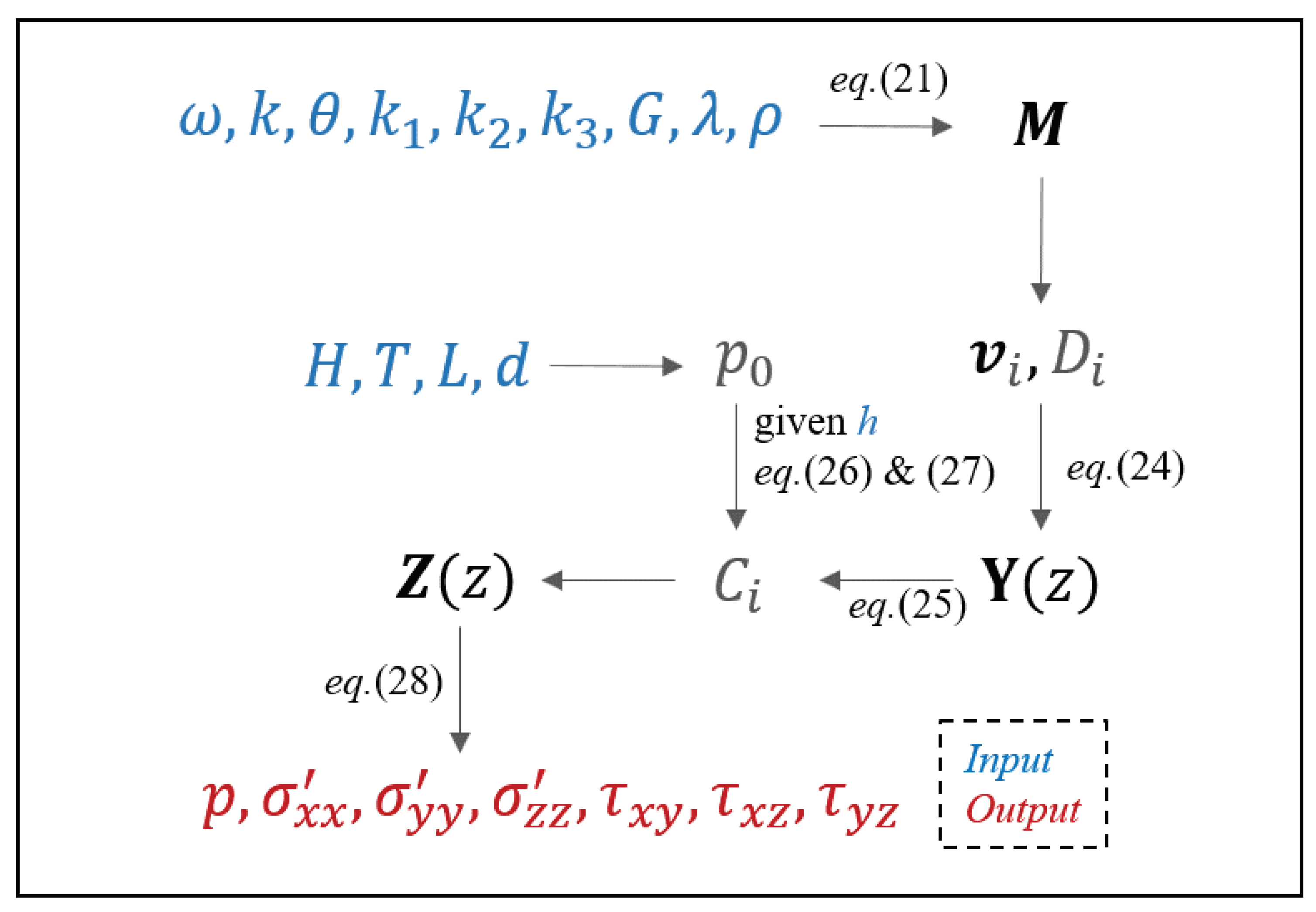
An implementation of the present process is illustrated as Figure 1, and the symbols are listed as Appendix A. The general solution is constructed as Equation (24) through $(\mathbf{M}-D_i\mathbf{E}){\mathbf{v}}_i=0$. Among the eight independent solutions, four solutions are directly computed in numerical form for four distinct complex eigenvalues and corresponding eigenvectors, and the other four solutions are obtained using two repeated real eigenvalues $D_i=\pm {\left(k^2-\rho {\omega }^2/G\right)}^{1/2}$, where two independent eigenvectors can be found numerically for each repeated eigenvalue. Then, the particular solutions are determined through the boundary condition of Equations (26) and (27), utilizing the transformation as Equation (25). Last, the desired wave-induced dynamic response in three-dimensional space, $\mathbf{z}={\left[p,{\sigma }_{xx}^{\prime },{\sigma }_{yy}^{\prime },{\sigma }_{zz}^{\prime },{\tau }_{xy},{\tau }_{xz},{\tau }_{yz}\right]}^T$, can be acquired as:

$$\mathbf{z}=\mathrm{Re}\left\{\mathbf{Z}\left(z\right)e^{\mathrm{i}\varphi (x,y,t)}\right\},$$

(28)

where $\mathbf{Z}\left(z\right)={\left[P\left(z\right),S_{xx}\left(z\right),S_{yy}\left(z\right),S_{zz}\left(z\right),S_{xy}\left(z\right),S_{xz}\left(z\right),S_{yz}\left(z\right)\right]}^T$.

3. Verification

To verify the three-dimensional anisotropic seabed response for the $u-p$ dynamic form, the present solution was compared with two benchmark analytical solutions considering QS approximation: the two-dimensional solutions of Yamamoto [15] and the three-dimensional solution of Hsu and Jeng [18]. It is noted that these two solutions were used for verification in many previous studies [18,22,25]. The solution of Yamamoto assumed isotropic permeability in the seabed ($k_1=k_3$) [15], while that of Hsu and Jeng considered anisotropic permeability and presented the result of the horizontal transverse isotropic seabed ($k_1=k_2>k_3$) [18].

Table 1. Parameters of water and soil.

Parameter	Value	Unit
Density of water, ${\rho }_f$	1000	$\mathrm{kg}/{\mathrm{m}}^3$
Bulk modulus of water, $K_w$	$2\times {10}^9$	Pa
Density of soil particles, ${\rho }_f$	2700	$\mathrm{kg}/{\mathrm{m}}^3$
Shear modulus of soil, G	${10}^7$	Pa
Poisson’s ratio, $\mu$	$1/3$
Porosity, n	$0.3$
Saturation, $S_r$	1

lists the fixed parameters used for the following verification and results in the next section. The other parameters for each case, including the seabed thickness h, soil permeability $k_i$, water depth d, wavelength L, wave period T, wave height H, and wave direction $\theta$, will be introduced later.

3.1. Comparison with the Two-Dimensional Solution of Yamamoto

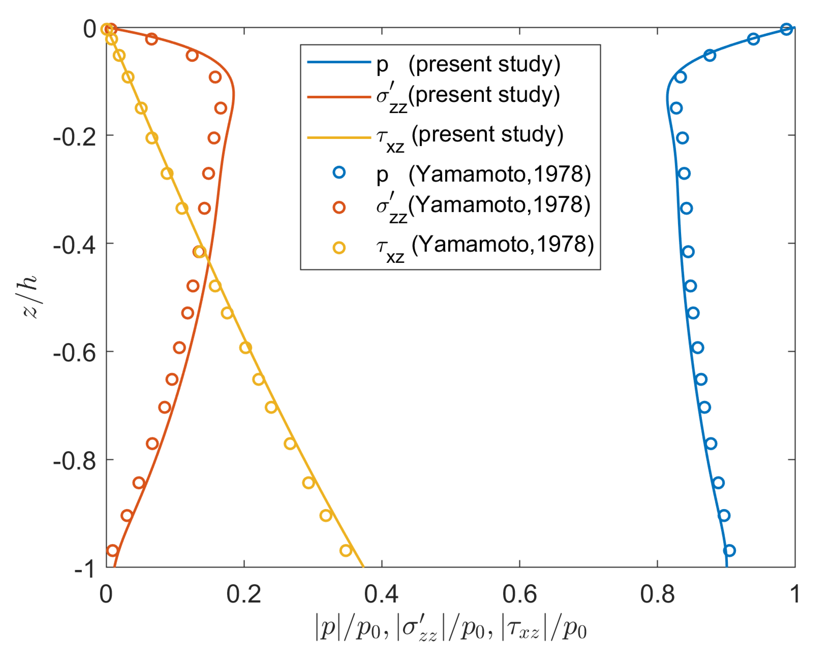
A comparison between the present solution and the solution of Yamamoto [15] is shown in Figure 2, and the following parameters were adopted: $h=25\mathrm{m}$, $d=70\mathrm{m}$, $L=312\mathrm{m}$, $H=24\mathrm{m}$, $T=15\mathrm{s}$, $\theta =0°$, and $k_1=k_2=k_3={10}^{-4}\mathrm{m}/\mathrm{s}$. It can be regarded as a fine sand case due to the low permeability. It is noted that Yamamoto [16] had verified his analytical solution of pore pressure by a physical hydraulic experiment. In Figure 2, the seabed responses of pore pressure p, vertical effective stress ${\sigma }_{zz}^{\prime }$, and shear stress ${\tau }_{xz}$ are compared through the vertical profile of maximum magnitude. $\left|p\right|$ denotes the maximum of p along the vertical coordinate z and equals the amplitude function in linear wave theory ($\left|p\right|=\left|P\right(z\left)\right|$). The result of the comparison has a good agreement and implies that the present solution can be used for the prediction of two-dimensional cases. Additionally, the result indicates that the permeability, whose direction is perpendicular to wave propagation ($k_2={10}^{-4}\mathrm{m}/\mathrm{s}$), has no effect on $\left|p\right|$, ${\sigma }_{zz}^{\prime }$, and ${\tau }_{xz}$.

3.2. Comparison with the Three-Dimensional Solution of Hsu and Jeng

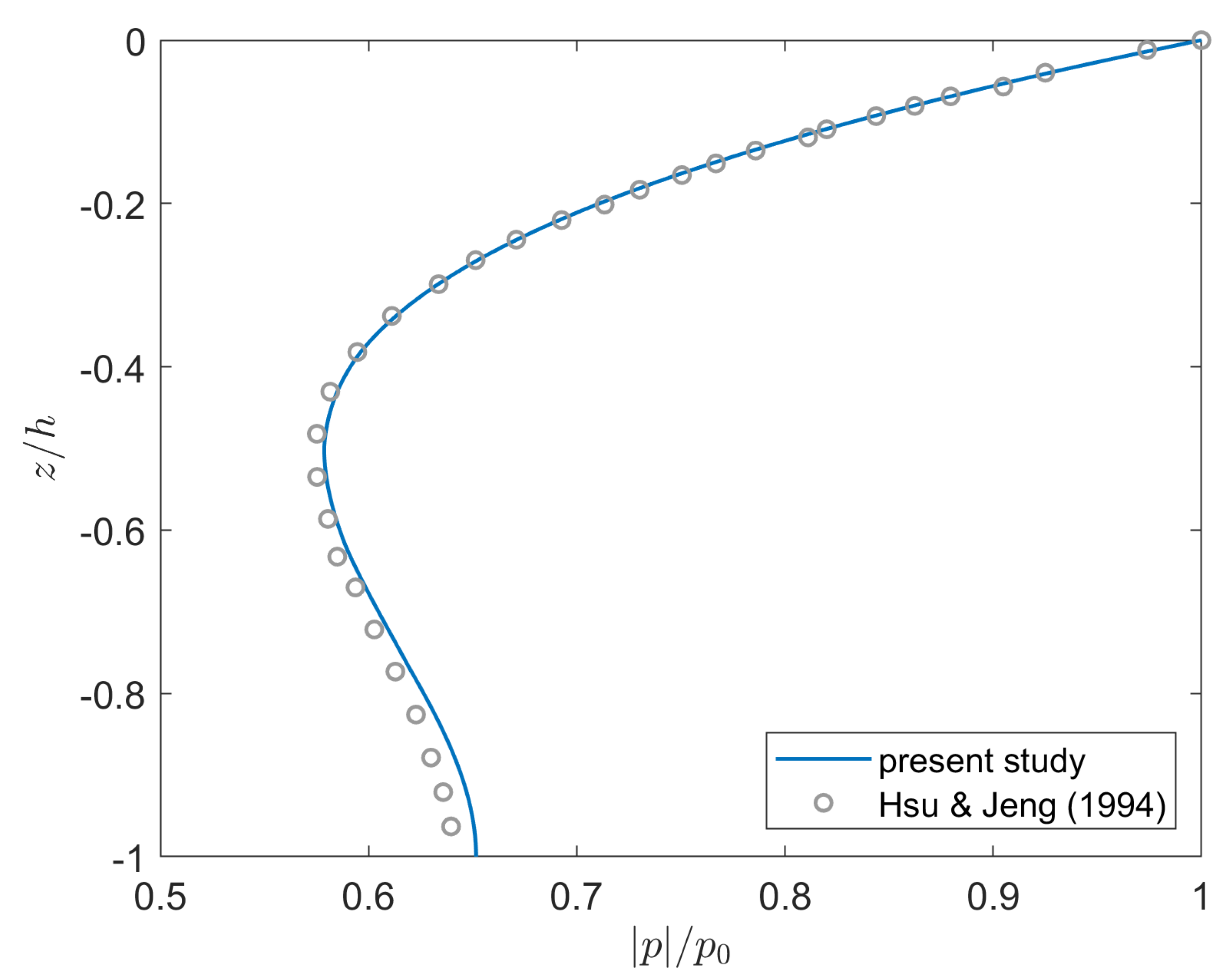
Figure 3 shows a comparison with the solution of Hsu and Jeng [18] and adopts the following parameters: $h=44.8\mathrm{m}$, $d=50\mathrm{m}$, $L=244\mathrm{m}$, $H=24\mathrm{m}$, $T=13.5\mathrm{s}$, $\theta =45°$, and $k_1=k_2=2.5k_3$, and $k_3={10}^{-2}\mathrm{m}/\mathrm{s}$ is the vertical permeability. This scenario considered an incident wave propagated in miter angle into a horizontal transverse isotropic seabed, whose horizontal permeability was two and a half times as much as the vertical permeability. It was a case of coarse sand because the high permeability and pore pressure naturally dissipate along the depth due to the thicker seabed. The present solution also agreed with the result of Hsu and Jeng [18]. Therefore, the present solution was verified by two previous solutions adopting $QS$ approximation with different permeabilities. As the wavelengths of the above two cases were quite long, there was little discrepancy between the results of the $u-p$ dynamic form and $QS$ approximation.

4. Results and Discussion

As the anisotropic permeability of soil is common in a natural environment, the present solution was suitable for investigating the effect of anisotropy on a three-dimensional dynamic seabed response for rapid soil behavior. In what follows, the effect of anisotropic permeability on three-dimensional seabed response is discussed in three parts. First, the seabed response under different wave periods for anisotropic permeability was performed to sketch the effect of the wave condition. Second, the seabed response for anisotropic permeability was compared with the results of isotropy and transverse isotropy to evaluate the error when the accurate directional permeability failed to be acquired. Third, the results of anisotropy and transverse isotropy for varied directions of the incident wave were compared, to discuss the effect of wave direction under anisotropic soil. In the following discussion, the material parameters listed in Table 1 were adopted, and the seabed environment had a water depth $d=70\mathrm{m}$ and seabed thickness $h=25\mathrm{m}$, as shown in Section 3.1.

Table 2. Case parameters.

No.	H (m)	T (s)	L (m)	d (m)	$\mathit{\theta }$ (${}^{\circ }$)	${\mathit{k}}_1$ (m/s)	${\mathit{k}}_2$ (m/s)	${\mathit{k}}_3$ (m/s)
1	24	10	155	70	30	0.10	0.05	0.01
2	24	15	312	70	30	0.10	0.05	0.01
3	24	20	462	70	30	0.10	0.05	0.01
4	24	15	312	70	0	0.10	0.05	0.01
5	24	15	312	70	60	0.10	0.05	0.01
6	24	15	312	70	90	0.10	0.05	0.01
7	24	15	312	70	0	0.05	0.05	0.01
8	24	15	312	70	30	0.05	0.05	0.01
9	24	15	312	70	60	0.05	0.05	0.01
10	24	15	312	70	90	0.05	0.05	0.01
11	24	15	312	70	30	0.01	0.01	0.01

lists the major parameters for each case including the wave condition (H, T, L, and d), wave direction $\theta$, and directional permeability ($k_1$, $k_2$, and $k_3$). The wave condition for wave period $T=15\mathrm{s}$ in Table 2, as well as the physical quantities of the material and seabed environment were a practical design condition of the North Sea, and this set of parameters was intensively applied in previous studies [15,16,27]. The other wave conditions for wave periods $T=10\mathrm{s}$ and $T=20\mathrm{s}$ represented the scenario under shorter and longer waves, respectively. It is noted that the range of the wave period from $T=10\mathrm{s}$ to $T=20\mathrm{s}$ belonged to the type of the ordinary gravity wave in wind wave theory [28]. Besides the wave parameters that determined the fluctuation of seabed pressure, the soil parameters may have a wide range of values for various materials, and some parameters may significantly affect the seabed response. For example, the shear modulus of the soil was an important parameter, owing to its extent, and saturation was another sensitive parameter that may change the result with a slight difference. The effects of rigidity and water content, as well as wave condition could be referred to Jeng and Cha [20] and Ulker et al. [21]. In this study, we focused on the effect of anisotropic permeability for different wave periods and wave directions on the seabed response in three-dimensional space.

4.1. Effect of the Wave Period on the Anisotropic Seabed

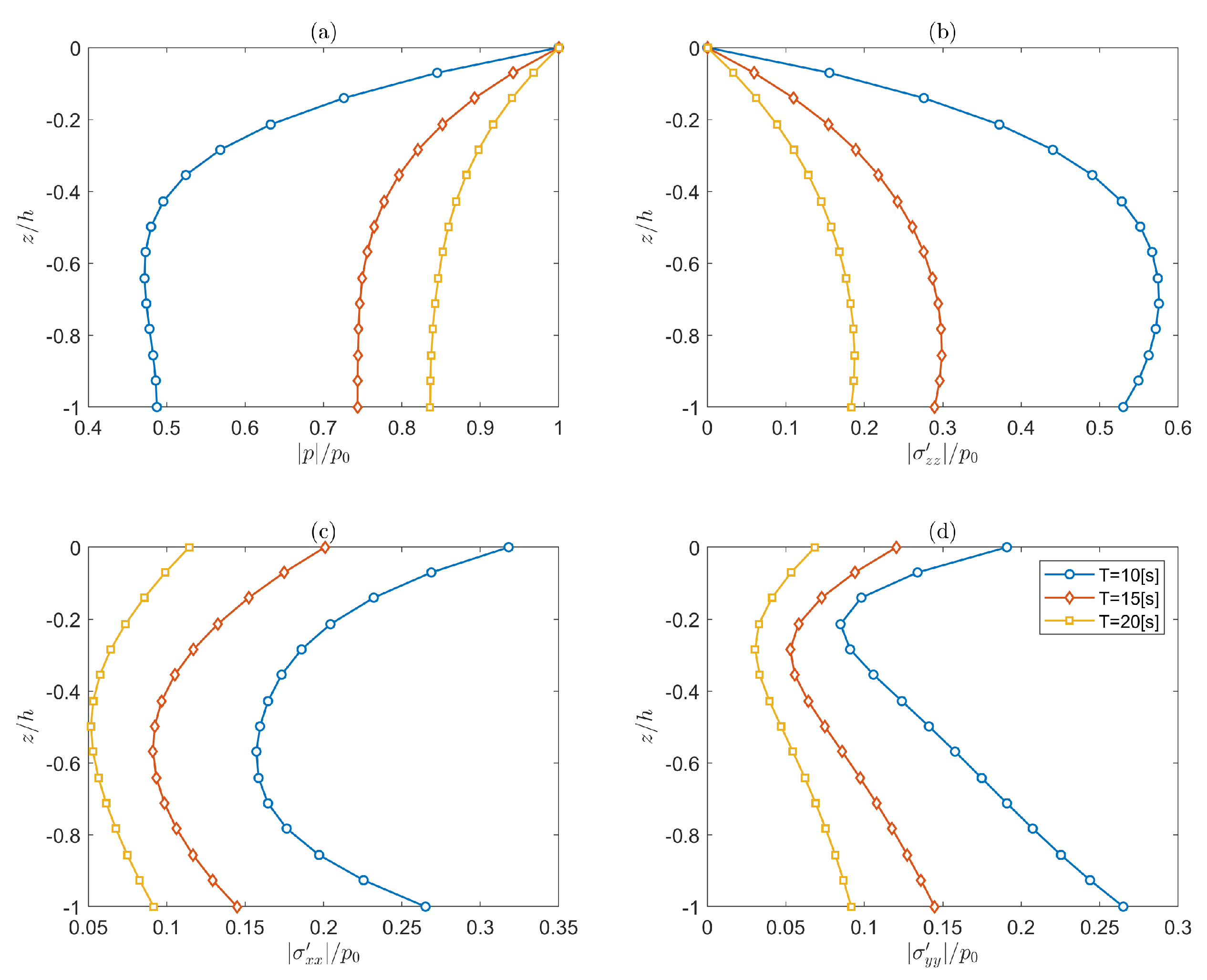
Considering that waves propagate in direction $\theta =30°$, three wave periods, $T=10\mathrm{s}$, $15\mathrm{s}$, and $20\mathrm{s}$, were selected for representing the range of wave conditions from short wave to long wave. The corresponding wavelengths were $L=155\mathrm{m}$ for $T=10\mathrm{s}$, $L=312\mathrm{m}$ for $T=15\mathrm{s}$, and $L=462\mathrm{m}$ for $T=20\mathrm{s}$, based on the linear wave theory. The anisotropic permeability was set as $k_1=0.1\mathrm{m}/\mathrm{s}$, $k_2=0.05\mathrm{m}/\mathrm{s}$, and vertical permeability $k_3=0.01\mathrm{m}/\mathrm{s}$. Figure 4 demonstrates the amplitude profiles of pore pressure and effective stresses for different wave periods. In Figure 4a,b, the amplitude of pore pressure decreases with depth, while that of vertical effective stress increases, and shorter waves have more reduction of $\left|p\right|$ and increment of ${\sigma }_{zz}^{\prime }$, as a higher frequency of the loading wave implied a rapid interaction between the soil and pore flow. A similar phenomenon was observed by Zhou et al. [29]. For longer waves $T=15\mathrm{s}$ and $T=20\mathrm{s}$, $\left|p\right|$ decreased monotonically, and the minimum of $\left|p\right|$ was on the bottom. For shorter waves $T=10\mathrm{s}$, the minimum $\left|p\right|/p_0=0.472$ occurred at the depth $z/h=-0.615$. On the other hand, the maximum of $|{\sigma }_{zz}^{\prime }|$ occurred at the upper soil layer for shorter waves. For $T=10\mathrm{s}$, $15\mathrm{s}$, and $20\mathrm{s}$, the maximum of $|{\sigma }_{zz}^{\prime }|$ was $|{\sigma }_{zz}^{\prime }|/p_0=0.576$, $0.299$, and $0.188$, which occurred at the depths $z/h=-0.692$, $-0.833$, and $-0.860$, respectively. When a periodic wave propagated, the soil tended to expand under a wave crest and contract under a wave trough. The soil contraction was accompanied with the build-up of excess pore pressure, particularly at the depth of a minimum $\left|p\right|$. For fine sands with low permeability, an excess pore pressure may build up on the upper soil layer to cause a risk of liquefaction. The amplitude profiles of horizontal effective stress $|{\sigma }_{xx}^{\prime }|$ for different wave periods are shown in Figure 4c, and that of $|{\sigma }_{yy}^{\prime }|$ is shown in Figure 4d. Both indicated that shorter waves had a greater magnitude of amplitude, and the minimum occurred in the middle layer. The maximum of $|{\sigma }_{xx}^{\prime }|$ occurred at the seabed surface, while that of $|{\sigma }_{yy}^{\prime }|$ appeared on the seabed bottom. In general, the amplitude profile of the seabed response for shorter waves varied dramatically with the depth, as compared to the longer ones, and the discrepancy between the profiles of the two shorter waves was much greater.

4.2. Comparison of Seabed Response for Anisotropic, Transverse Isotropic, and Isotropic Permeabilities

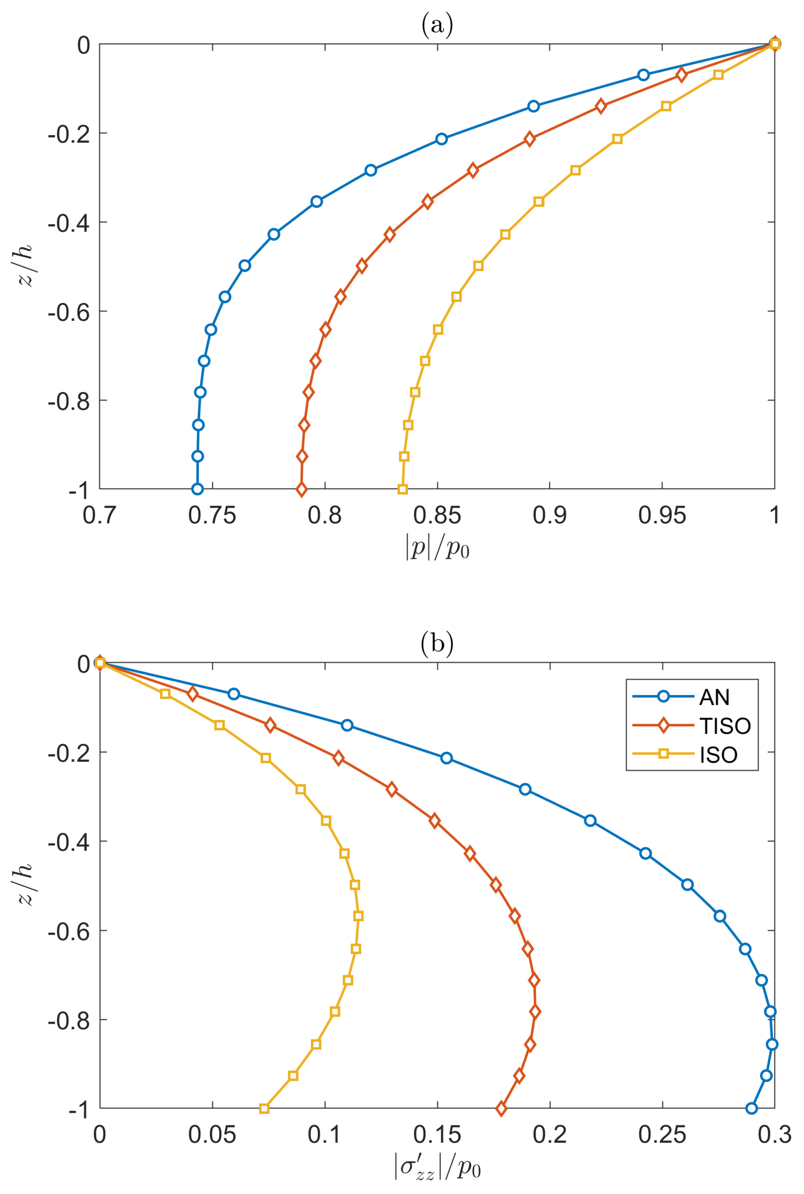
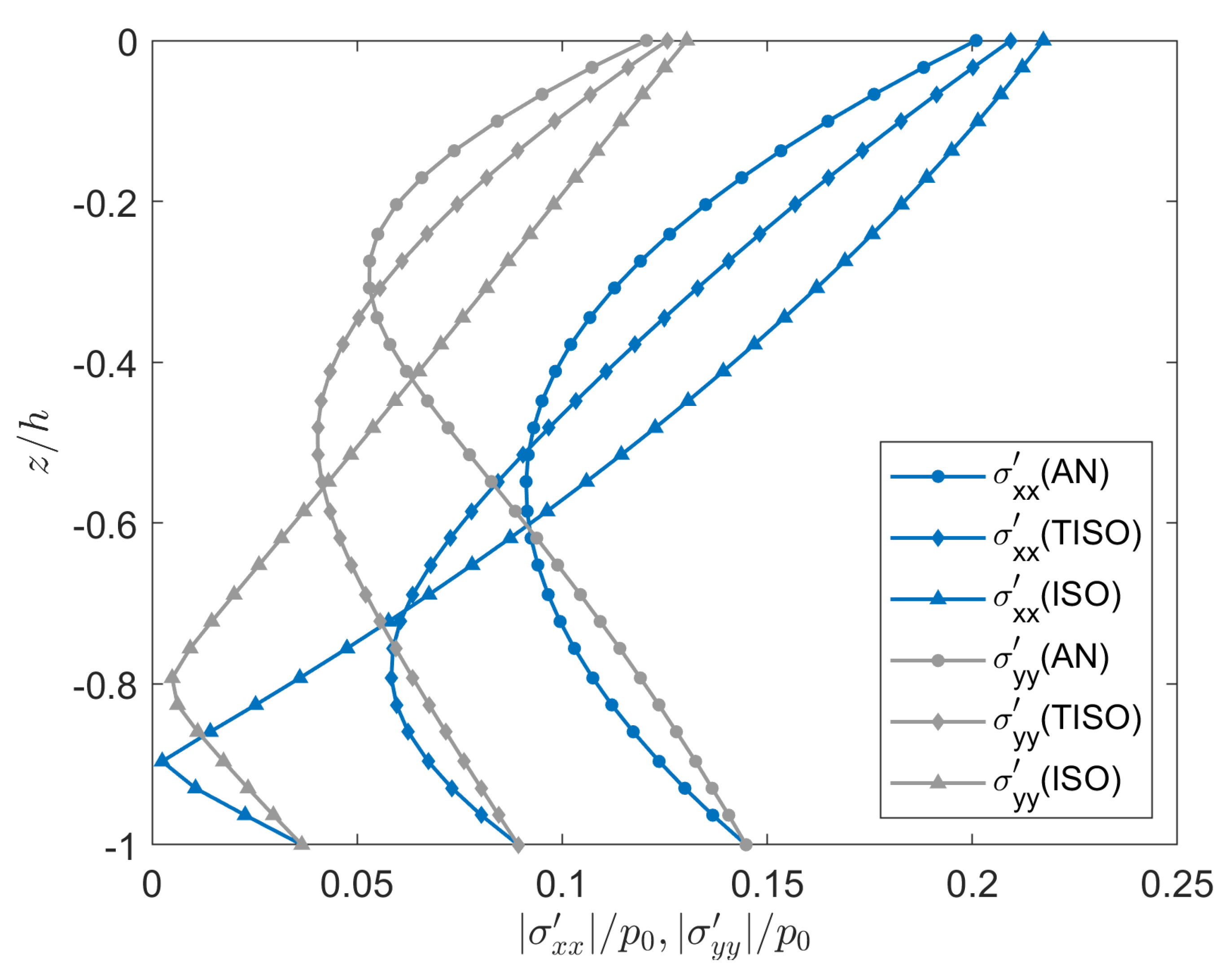
The seabed response for anisotropic permeability was compared with two reduced permeabilities: transverse isotropy and isotropy. Except for the permeability of isotropy and transverse isotropy, the adopted parameters were identical to those used in Section 4.1 for wave conditions $T=15\mathrm{s}$, $L=312\mathrm{m}$, and $\theta =30°$. The transverse isotropic permeability employed $k_1=k_2=0.05\mathrm{m}/\mathrm{s}$ and $k_3=0.01\mathrm{m}/\mathrm{s}$, while the isotropic permeability used $k_1=k_2=k_3=0.01\mathrm{m}/\mathrm{s}$. For convenience, in the following legend of the figure, “AN” denotes the seabed response for anisotropic permeability, “TISO” denotes that for transverse isotropic permeability, and “ISO” denotes that for isotropic permeability. Figure 5 shows a comparison of the amplitude profile of pore pressure and vertical effective stress among these three permeabilities. In Figure 5a, the amplitude profiles of pore pressure $\left|p\right|$ for transverse isotropy and isotropy attenuate more slowly with depth than those for anisotropic permeability. All of the minima of $\left|p\right|$ occurred on the seabed bottom, where the relative error of $\left|p\right|$ was $6.2\%$ for transverse isotropic permeability and $12.3\%$ for isotropic permeability. In Figure 5b, the amplitude profile of vertical effective stress $|{\sigma }_{zz}^{\prime }|$ for anisotropic permeability is greater than the others. On the seabed bottom, the relative error of $|{\sigma }_{zz}^{\prime }|$ was $38.4\%$ for transverse isotropic permeability and $74.8\%$ for the isotropic one. For anisotropic permeability, the maximum of $|{\sigma }_{zz}^{\prime }|/p_0$ was $0.299$, and its depth was $z/h=-0.833$. For transverse isotropic permeability, the maximum of $|{\sigma }_{zz}^{\prime }|/p_0$ was $0.194$, and its depth was $z/h=-0.763$. For isotropic permeability, the maximum of $|{\sigma }_{zz}^{\prime }|/p_0$ was $0.115$, and its depth was $z/h=-0.575$. Figure 6 shows a comparison of horizontal effective stresses ${\sigma }_{xx}^{\prime }$ and ${\sigma }_{yy}^{\prime }$. The amplitude profiles for isotropic and transverse isotropic permeabilities varied significantly as compared to those for anisotropic permeability, and the variation was sorted in descending order as isotropy>transverse isotropy>anisotropy. An interesting observation was that the amplitudes of ${\sigma }_{xx}^{\prime }$ and ${\sigma }_{yy}^{\prime }$ coincided on the seabed bottom for each type of permeability. This was because the amplitudes on the seabed bottom reduced as $S_{xx}(-h)=S_{yy}(-h)=\lambda {\left.{\dot{U}}_z\left(z\right)\right|}_{z=-h}$ after substituting the boundary condition into Equation (25). Note that the discrepancy between $|{\sigma }_{xx}^{\prime }|$ and $|{\sigma }_{yy}^{\prime }|$ resulted from the angle of wave direction $\theta =30°$, rather than the different permeabilities in the coordinates, and the amplitude profiles of horizontal effective stress coincided with each other when $\theta =45°$.

4.3. Effect of Wave Direction on Anisotropic Permeability

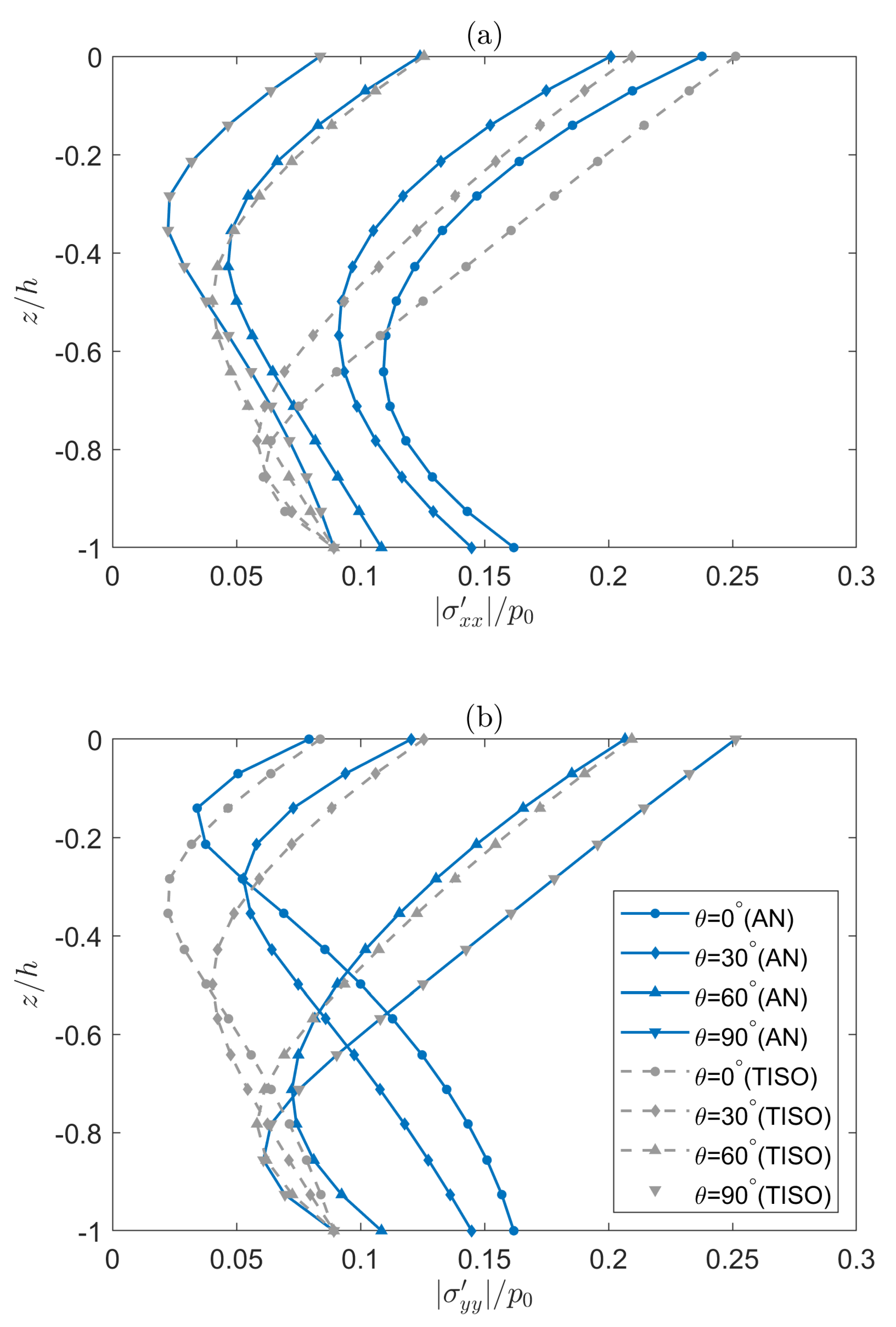
Adopting the same parameter of wave condition and the permeability for anisotropy and transverse isotropy used in Section 4.2, the seabed responses of different angles of wave direction were compared between the two permeabilities. The amplitude profiles of pore pressure and vertical effective stress are shown in Figure 7. For transverse isotropic permeability, both $\left|p\right|$ and $|{\sigma }_{zz}^{\prime }|$ were independent of the wave direction, and $\theta =30°$ was chosen as a representative. The result of transverse isotropic permeability was identical to that of anisotropic permeability for $\theta =90°$, whose wave direction was parallel to that having the same value of permeability $k_2=0.05\mathrm{m}/\mathrm{s}$. For anisotropic permeability, when the angle of wave direction $\theta$ increased, both the reduction of $\left|p\right|$ and the increment of $|{\sigma }_{zz}^{\prime }|$ along the depth were attenuated. In other words, when the wave direction was parallel to the direction having the greater horizontal permeability, the amplitude profiles of pore pressure and vertical effective stress had the greatest dissipation and increment, respectively. Figure 8 shows the amplitude profile of horizontal effective stresses ${\sigma }_{xx}^{\prime }$ and ${\sigma }_{xx}^{\prime }$, respectively. In Figure 8a, the amplitude profile decreases when the angle of the wave direction increases, and the amplitude profile for anisotropic permeability coincides with that for the transverse isotropic one when $\theta =90°$. Moreover, the discrepancy of $|{\sigma }_{xx}^{\prime }|$ between the two permeability types was the greatest when $\theta =0°$. In Figure 8b, the amplitude on the seabed surface increases with $\theta$. For anisotropic permeability, the amplitude of ${\sigma }_{yy}^{\prime }$ on the seabed bottom decreased when $\theta$ increased. However, for transverse isotropic permeability, all $|{\sigma }_{yy}^{\prime }|/p_0$ at $z=-h$ coincided at the same value of approximately $0.09$. This was attributable to the fact that $|{\sigma }_{zz}^{\prime }|$ was independent of the wave direction for transverse isotropic permeability, as shown in Figure 7b, so its derivative of $S_{zz}$ was also independent of the wave direction. Consequently, both $|{\sigma }_{xx}^{\prime }|$ and $|{\sigma }_{yy}^{\prime }|$ on the seabed bottom were independent of the wave direction for the case of transverse isotropy due to the relation of $S_{xx}(-h)=S_{yy}(-h)=\lambda {\left.{\dot{U}}_z\left(z\right)\right|}_{z=-h}$.

5. Conclusions

An analytical solution was developed for investigating three-dimensional wave-induced dynamic responses in the seabed of anisotropic permeability. The analytical solution was based on the $u-p$ dynamic form, which considered the effect of inertia force on the soil skeleton. A first-order ODE in matrix form was derived to deal with this problem as an eigenvalue problem rather than a set of four second-order ODEs, which were used for solving the problems in the previous literature. To deal with the complicated eigenvector problem involved in the general solution, numerical computation was used through the QZ algorithm, and the error was found to be less than ${10}^{-8}$. A process was proposed to implement the present solution for the desired dynamic response. According to the performed analyses and presented comparisons, the following conclusions could be drawn:

• The present solution considered the inertial force of the soil skeleton for a rapid soil behavior and for predicting three-dimensional dynamic responses comprising the pore pressure and stresses for anisotropic permeability. In addition, the verification of the present solution in comparison with two existing solutions with two different permeabilities showed a good agreement.
• In general, the amplitude of pore pressure decreased with depth, while that of vertical effective stress increased, and a shorter wave period had greater reduction of $\left|p\right|$ and increment of ${\sigma }_{zz}^{\prime }$ due to the rapid interaction between the soil and pore flow. For horizontal effective stresses, both ${\sigma }_{xx}^{\prime }$ and ${\sigma }_{yy}^{\prime }$ showed that shorter waves had a greater magnitude of amplitude.
• In the comparison between the seabed responses for anisotropic permeability and the transverse isotropic and isotropic ones, the amplitude profiles of pore pressure for transverse isotropy and isotropy attenuated more slowly with depth as compared to anisotropic permeability. All of the minima of $\left|p\right|$ occurred on the seabed bottom, where the relative error of $\left|p\right|$ on the seabed bottom was $6.2\%$ for transverse isotropic permeability and $12.3\%$ for isotropic permeability. The amplitude profile of the vertical effective stress for anisotropic permeability was greater than that of transverse isotropy and isotropy. On the seabed bottom, the relative error of $|{\sigma }_{zz}^{\prime }|$ was $38.4\%$ for transverse isotropic permeability and $74.8\%$ for isotropic permeability. The amplitude profiles of horizontal effective stresses ${\sigma }_{xx}^{\prime }$ and ${\sigma }_{yy}^{\prime }$ for isotropic and transverse isotropic permeabilities varied significantly as compared to those for anisotropic permeability, and the variation was sorted in descending order as isotropy >transverse isotropy > anisotropy.
• For anisotropic permeability, when the wave direction was parallel to the direction having higher horizontal permeability, the amplitude profiles of pore pressure and vertical effective stress had the greatest dissipation and increment, respectively. On the other hand, for transverse isotropic permeability, both pore pressure and vertical effective stress were independent of the wave direction.
• It was shown that the horizontal effective stresses ${\sigma }_{xx}^{\prime }$ and ${\sigma }_{yy}^{\prime }$ were identical on the seabed for any permeability, and for transverse isotropic permeability, the magnitudes of ${\sigma }_{xx}^{\prime }$ and ${\sigma }_{yy}^{\prime }$ on the seabed were independent of the wave direction.
• Seabed instabilities including liquefaction and shear failure are other important issues in ocean environment. The present solution can be utilized on these problems and has potential to shed light on the underlying mechanisms.

References

- Ye, J.; Jeng, D.; Wang, R.; Zhu, C. A 3-D semi-coupled numerical model for fluid-structures-seabed-interaction (FSSI-CAS 3D): Model and verification. J. Fluids Struct. 2013, 40, 148–162. [Google Scholar] [CrossRef]
- Ai, Z.Y.; Hu, Y.D. Multi-dimensional consolidation of layered poroelastic materials with anisotropic permeability and compressible fluid and solid constituents. Acta Geotech. 2015, 10, 263–273. [Google Scholar] [CrossRef]
- Pulko, B.; Logar, J. Fully coupled solution for the consolidation of poroelastic soil around elastoplastic stone column. Acta Geotech. 2017, 12, 869–882. [Google Scholar] [CrossRef]
- Wang, G.; Chen, S.; Liu, C.; Shao, K.; Liu, Q. Wave-Induced Dynamic Response and Liquefaction of Transversely Isotropic Seabed. Int. J. Geomech. 2020, 20, 04019192. [Google Scholar] [CrossRef]
- Sui, T.; Zhang, C.; Guo, Y.K.; Zheng, J.H.; Jeng, D.S.; Zhang, J.S.; Zhang, W. Three-dimensional numerical model for wave-induced seabed response around mono-pile. Ships Offshore Struc. 2015, 11, 667–678. [Google Scholar] [CrossRef] [Green Version]
- Li, Y.; Ong, M.C.; Tang, T. A numerical toolbox for wave-induced seabed response analysis around marine structures in the OpenFOAM® framework. Ocean. Eng. 2019, 106678. [Google Scholar] [CrossRef]
- Asumadu, R.; Zhang, J.; Zhao, H.Y.; Osei-Wusuansa, H. A 3D numerical analysis of wave-induced seabed response around a monopile structure. Geomech. Geoeng. 2019, 1–21. [Google Scholar] [CrossRef]
- Li, H.; Wang, S.; Chen, X.; Hu, C.; Liu, J. Numerical study of scour depth effect on wave-induced seabed response and liquefaction around a pipeline. Mar. Georesources Geotechnol. 2019, 1–12. [Google Scholar] [CrossRef]
- Terzaghi, K. Erdbaumechanik auf Bodenphysikalischer Grundlage; Deuticke: Wien, Austria, 1925. [Google Scholar]
- Biot, M.A. General theory of three-dimensional consolidation. J. Appl. Phys. 1941, 12, 155–164. [Google Scholar] [CrossRef]
- Biot, M.A. Mechanics of deformation and acoustic propagation in porous media. J. Appl. Phys. 1962, 33, 1482–1498. [Google Scholar] [CrossRef]
- Verruijt, A. Elastic Storage of Aquifers. In Flow Through Porous Media; De Wiest, R.J.M., Ed.; Academic Press: New York, NY, USA, 1969; pp. 331–376. [Google Scholar]
- Mei, C.C.; Foda, M.A. Wave-induced responses in a fluid-filled poro-elastic solid with a free surface—A boundary layer theory. Geophys. J. R. Astron. Soc. 1981, 66, 597–631. [Google Scholar] [CrossRef]
- Madsen, O.S. Wave-induced pore pressures and effective stresses in a porous bed. Géotechnique 1978, 28, 377–393. [Google Scholar] [CrossRef]
- Yamamoto, T. Sea bed instability from waves. In Proceedings of the 10th Offshor Technology Conference, Houston, TX, USA, 30 April–3 May 1978; ASCE: Houston, TX, USA, 1978; pp. 1819–1828. [Google Scholar] [CrossRef]
- Yamamoto, T.; Koning, H.L.; Sellmeijer, H.; Hijum, E.V. On the response of a poro-elastic bed to water waves. J. Fluid Mech. 1978, 87, 193–206. [Google Scholar] [CrossRef]
- Hsu, J.R.C.; Jeng, D.S.; Tsai, C.P. Short-crested wave-induced soil response in a porous seabed of infinite thickness. Int. J. Numer. Anal. Met. 1993, 17, 553–576. [Google Scholar] [CrossRef]
- Hsu, J.R.C.; Jeng, D.S. Wave-induced soil response in an unsaturated anisotropic seabed of finite thickness. Int. J. Numer. Anal. Methods Geomech. 1994, 18, 785–807. [Google Scholar] [CrossRef]
- Zienkiewicz, O.C.; Chang, C.T.; Bettess, P. Drained, undrained, consolidating and dynamic behaviour assumptions in soils. Géotechnique 1980, 30, 385–395. [Google Scholar] [CrossRef]
- Jeng, D.S.; Cha, D.H. Effects of dynamic soil behavior and wave non-linearity on the wave-induced pore pressure and effective stresses in porous seabed. Ocean Eng. 2003, 30, 2065–2089. [Google Scholar] [CrossRef]
- Ulker, M.; Rahman, M.; Jeng, D.S. Wave-induced response of seabed: Various formulations and their applicability. Appl. Ocean Res. 2009, 31, 12–24. [Google Scholar] [CrossRef]
- Hsu, C.J.; Chen, Y.Y.; Tsai, C.C. Wave-induced seabed response in shallow water. Appl. Ocean Res. 2019, 89, 211–223. [Google Scholar] [CrossRef]
- Zhang, C.; Sui, T.; Zheng, J.H.; Xie, M.X.; Nguyen, V.T. Modelling wave-induced 3D non-homogeneous seabed response. Appl. Ocean Res. 2016, 61, 101–114. [Google Scholar] [CrossRef]
- Jeng, D.S. Wave dispersion equation in a porous seabed. Ocean Eng. 2001, 28, 1585–1599. [Google Scholar] [CrossRef]
- Ye, J.H.; Jeng, D.S. Response of Porous Seabed to Nature Loadings: Waves and Currents. J. Eng. Mech. 2012, 138, 601–613. [Google Scholar] [CrossRef]
- Moler, C.B.; Stewart, G.W. An Algorithm for Generalized Matrix Eigenvalue Problems. SIAM J. Numer. Anal. 1973, 10, 241–256. [Google Scholar] [CrossRef]
- Moshagen, H.; Torum, A. Wave Induced pressures in permeable seabeds. J. Waterw. Port Coast. Ocean Eng. 1975, 101, 49–57. [Google Scholar]
- Munk, W. Origin and generation of waves. In Proceedings of the 1st Conf. Coastal Engineering, Long Beach, CA, USA, 1 January 1950. [Google Scholar] [CrossRef] [Green Version]
- Zhou, X.L.; Zhang, J.; Wang, J.H.; Xu, Y.F.; Jeng, D.S. Stability and liquefaction analysis of porous seabed subjected to cnoidal wave. Appl. Ocean. Res. 2014, 48, 250–265. [Google Scholar] [CrossRef]
Figure 1.
Schematic diagram of the steps in the implementation process.
Figure 2.
Amplitude profile of pore pressure p, vertical effective stress , and shear stress for the isotropic case.
Figure 3.
Amplitude profile of pore pressure p for the horizontal transverse isotropic case.
Figure 4.
Effect of wave period on (a) pore pressure p and effective stresses (b) , (c) , and (d) along the z-axis for anisotropic permeability (, and 20 s correspond respectively to Cases 1, 2, and 3).
Figure 5.
Comparison of (a) pore pressure p and (b) vertical effective stress for anisotropic (AN), transverse isotropic (TISO), and isotropic (ISO) permeabilities (AN, TISO, and ISO correspond respectively to Cases 2, 8, and 11).
Figure 6.
Comparison of horizontal effective stresses and for AN, TISO, and ISO permeabilities (AN, TISO, and ISO correspond respectively to Cases 2, 8, and 11).
Figure 7.
Comparison of (a) pore pressure p and (b) vertical effective stress for different wave directions between AN and TISO permeabilities (for the AN cases, , and 90° correspond respectively to Cases 4, 2, 5, and 6; the TISO of corresponds to Case 8).
Figure 8.
Comparison of horizontal effective stresses (a) and (b) for different wave directions between AN and TISO permeabilities (for the AN cases, , and 90° correspond respectively to Cases 4, 2, 5, and 6; for the TISO cases, , and 90° correspond respectively to Cases 7, 8, 9, and 10).