Detecting Pattern Anomalies in Hydrological Time Series with Weighted Probabilistic Suffix Trees

Abstract

Anomalous patterns are common phenomena in time series datasets. The presence of anomalous patterns in hydrological data may represent some anomalous hydrometeorological events that are significantly different from others and induce a bias in the decision-making process related to design, operation and management of water resources. Hence, it is necessary to extract those “anomalous” knowledge that can provide valuable and useful information for future hydrological analysis and forecasting from hydrological data. This paper focuses on the problem of detecting anomalous patterns from hydrological time series data, and proposes an effective and accurate anomalous pattern detection approach, TFSAX_wPST, which combines the advantages of the Trend Feature Symbolic Aggregate approximation (TFSAX) and weighted Probabilistic Suffix Tree (wPST). Experiments with different hydrological real-world time series are reported, and the results indicate that the proposed methods are fast and can correctly detect anomalous patterns for hydrological time series analysis, and thus promote the deep analysis and continuous utilization of hydrological time series data.

1. Introduction

In the era of Big Data, new satellite, space, airborne, shipborne and ground-based remote sensing systems, as well as Internet of Things (IoT) devices, are ubiquitous, producing data rapidly and continuously, which lead to hydrological time series being acquired at a breathless pace, both in size and variety [1,2]. However, due to measurement/manual operation errors, instrument failure, changes in natural laws caused by human activities or hydrological evolution, there is a large number of “anomalous” data in hydrological time series. Undoubtedly, those “anomalous” data will significantly affect the models related to flood forecasting and hydrological analysis, and lead to potentially incomplete or inaccurate results [3]. Therefore, detecting those “anomalies” in hydrological datasets is becoming an important and urgent task for hydrology and information researchers [4].

Anomalies are individuals that behave in an unexpected way or feature abnormal properties [5]. According to the literature [6,7], anomalies in time series can be divided into point anomalies and pattern anomalies, and the problem of finding those unexpected individual points or patterns is referred to as anomaly detection. For hydrological time series data, many researchers have proposed different anomaly detection algorithms from different application aspects to address “anomalous” variables [8,9,10,11,12,13,14,15]. However, those methods pay more attention to detect point anomalies to improve hydrological data quality rather than mine potentially meaningful pattern anomalies within a given time series.

Pattern anomalies in hydrologic time series may be related to disastrous hydrometeorological events (flood or drought) within a period of time [16]. Therefore, detecting and analyzing pattern anomalies in hydrological time series is helpful to discover the law of a hydrological process, to provide decision support for early warning and prevention of flood and drought disasters, and to reduce economic and social losses. However, there are very few studies focusing on hydrological time series pattern anomaly detection. Moreover, due to the fact that the nature of the time series and anomalies are fundamentally divergent in different domains, it is hard to apply those pattern anomaly detection algorithms that are effective in other areas [17,18,19,20,21,22] to the hydrology field.

Therefore, this paper proposes a novel pattern anomaly detection algorithm, TFSAX_wPST, to detect hydrological time series pattern anomalies. The algorithm first uses the Trend Feature Symbolic Aggregate approximation (TFSAX) [23] to discretize original time series into symbolic time series, then proposes the weighted Probability Suffix Tree (wPST) to construct the symbol sequence obtained by the above steps, and thus top-k pattern anomalies are analyzed and verified from the candidate pattern anomalies set based on the sequence that was pruned during the wPST construction process. Experimental results show TFSAX_wPST can accurately detect pattern anomalies in hydrological time series and thus provides technical and application support for hydrological time series data analysis and decision-making.

2. Related Work

2.1. Time Series Pattern Anomaly Detection

A time series pattern anomaly represents a pattern with anomalous behavior that is significantly different from other patterns within a given time series. Generally, a pattern may contain a collection of data instances, where each single data instance is not anomalous; however, the combination of them may be an anomaly and implies more important information [6]. For example, it may be a normal condition if the mean daily water level of a station on some day of July is lower than its mean water level over the same period in history. But it may indicate an anomalous pattern (drought event) when the mean daily water level of all 31 days in July at this station is lower than its mean water level over the same period in history. Therefore, detecting and analyzing pattern anomalies that contain more interesting information is more meaningful and valuable [6].

A time series pattern (TSP) represents a certain characteristic trend within a given time series, which may be a statistical characteristics metric (e.g., maximum, minimum or mean values of a segment) or mathematical transformation (e.g., Fourier transform). Formally, given a time series TS, the pattern of TS can be formally represented as a pattern–time tuple:

TS = <(m₁, t₁), (m₂, t₂) … (m_i, t_i)…(m_N, t_N)> i = 1,2…N

(1)

where tuple (m_i, t_i) indicates that the pattern of TS is m₁ during 0–t₁, m₂ during t₁–t₂, m_N during t_{N − 1}–t_N, and so on and so forth.

Researchers use Novelty Pattern, Surprise Pattern, Discord, Novel Event and Aberrant Behavior to describe anomaly patterns, and thus design window-based [6,24], similarity-based [25,26], symbolic representation-based [21,27] and model-based [28,29,30,31] algorithms to detect the tuples (m_i, t_i) on a given time series TS that met the definition of the pattern anomaly based on different application areas and purposes [32].

Wan [33] proposed the FP_SAX (Feature Points Symbolic Aggregate Approximation) approach to improve the selection of feature points, and then detect those patterns that have the top-k distance measured by Symbol Distance-based Dynamic Time Warping (SD_DTW) as anomalous patterns on hydrological time series. Zhang [34] proposed the distance-based anomalous patterns detection method by improving the selection of feature points in FP_SAX [33] and its distance measurement method. Those approaches have a lower fitting error and higher accuracy in the task of anomalous hydrological time series patterns mining, but how to choose a proper number (N) of feature points and the anomaly determination threshold will affect the detection accuracy and results of the algorithm. Wu et.al [35] used the quantile perturbation method (QPM) to reveal rainfall time series anomalies and changes over the Yellow River Basin due to the fragile ecosystem and rainfall-related disasters. The QPM method is a tool for analyzing extreme values and effective for the identification and analysis of extreme meteorological events. However, it is relatively weak for the detection of ordinary anomalous events.

For detecting pattern anomalies in time series, some existing methods in the literature reduce the problem to a point anomaly detection problem before solving it [11]. In some other methods, pattern anomalies are detected by using different machine learning and data mining approaches [3]. Markov Models (MM) [36] and their variants [29,31] are the popular machine learning approaches extensively used for pattern anomalies detection in time series. In the next section, we briefly study PST-based anomaly detection approaches.

2.2. PST-Based Anomaly Detection

The Markov model is a powerful finite state machine and widely used in sequence modeling. The Markov approaches are used in several studies to solve anomaly detection problems with the idea that an odd behavior might be represented not only by a single observation, but also by a series of consecutive observations [36]. The Probabilistic Suffix Tree (PST) is a compact representation of the Variable Order Markov Model (VMM) and uses a suffix tree as its storage structure. It originally comes from Probabilistic Suffix Automata (PSA) [37] and is believed to have a more memory efficient representation than the PSA. Hence, it has been used in several domains as an efficient approach for classifying sequences [38,39].

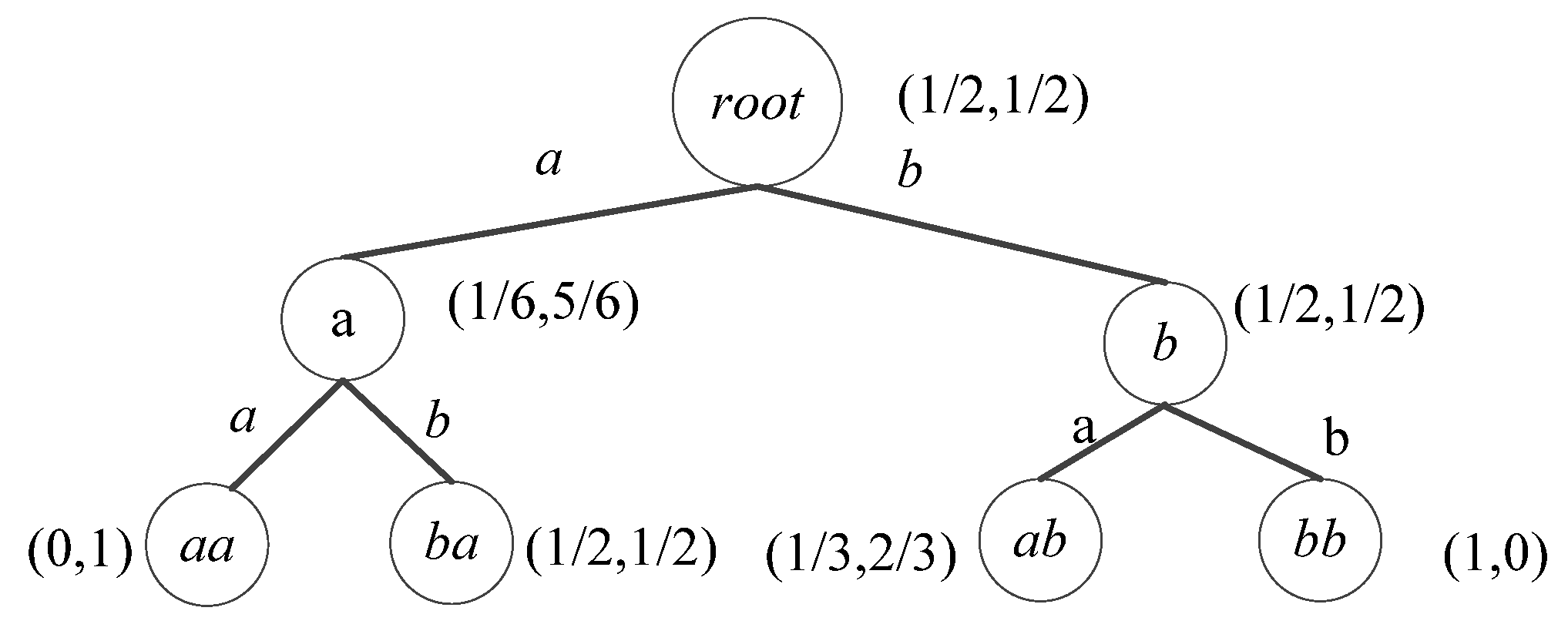
Figure 1 is an example of a PST corresponding to string s₁: abbabbabaaba over the alphabet Σ = {a, b} and tree depth L = 2. In PST, each edge is labelled by a unique symbol σ in Σ. Each node has at most two (|Σ|) children and records a string representing a path from the node to the root. The node also records a probability distribution vector corresponding to the conditional probabilities of seeing a symbol right after the label string in the dataset [40]. PST models the normal behave using the maximum likelihood criterion likelihood ratio. For a given sequence S and its PST T, the total likelihood-ratio of the observations can be expressed mathematically as L = Pr (S|T). If the probability of the observation sequence given the model has the largest likelihood ratio (or exceeding a certain preset threshold θ), then an anomaly is detected [29,41].

However, PST is a sequence statistical model based on VMM. It inherits the shortcomings, such as losing important sequence information and reducing detection accuracy of the VMM in anomaly detection tasks [42]. For subsequence A: abbabbabaaba, and B: abbabaaaaaaa, the probability that seeing a right after event ab in subsequence A (P_A(a|ab)) is equal to that of subsequence B (P_B(a|ab)). However, the frequency of event ab occurring in A (P_A(ab) = 4/11) is higher than that in B (P_B(ab) = 2/11). Hence, if it only uses probability to represent the sequence for anomaly detection tasks, it may lead to an erroneous analysis result.

Therefore, we propose a novel wPST model to better descript and accurately distinguish different time series sequences; thus, we give here a formal definition for pattern anomaly based on wPST to define the detection boundary and detection target for our anomaly detection algorithm.

3. A Novel Time Series Anomaly Detection Approach TFSAX_wPST

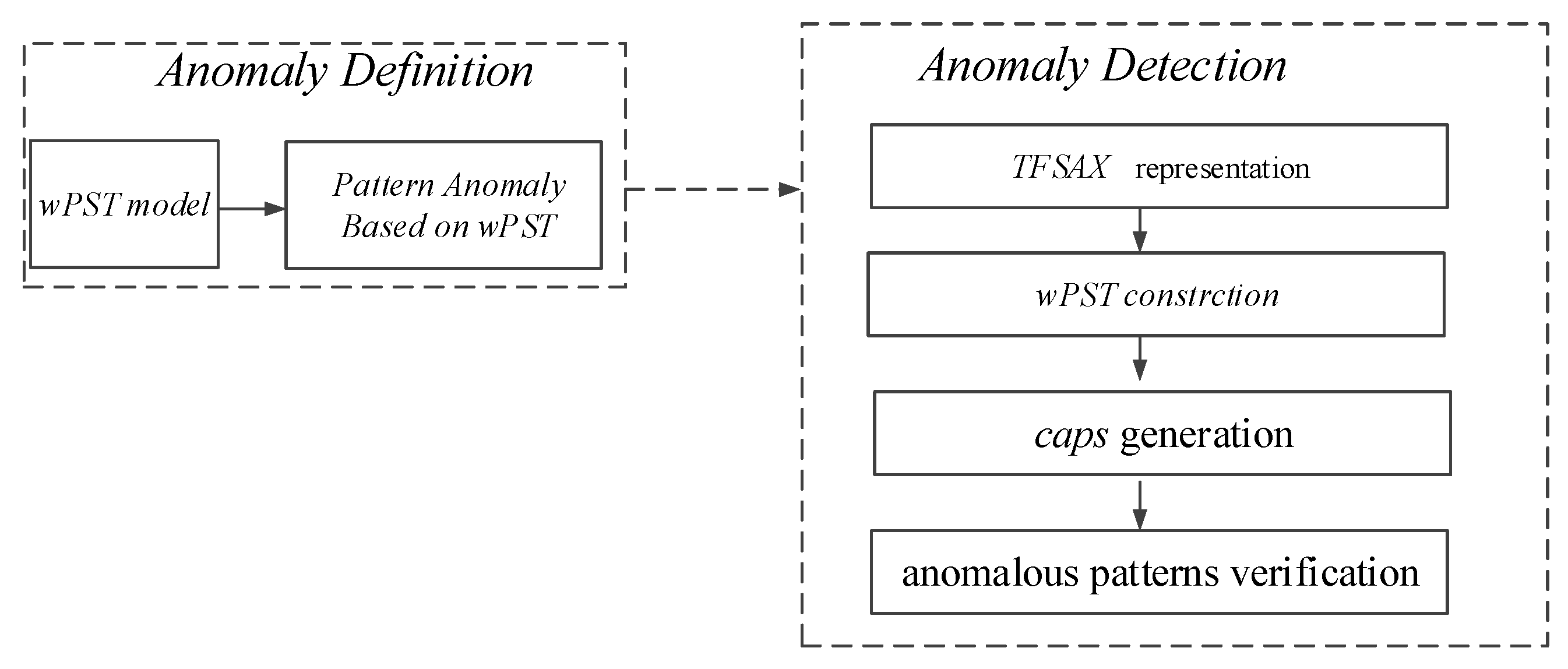
In this section, we propose a novel time series pattern anomaly detection approach, TFSAX_ wPST. Firstly, we propose a novel wPST model as the structure to store symbol sequences and give a formal definition for a hydrological time series pattern anomaly based on wPST. Then, we conduct a novel time series anomaly detection approach TFSAX_wPST to detect pattern anomalies within a given hydrological time series. TFSAX_wPST can be performed as in Figure 2.

(1) Anomaly Definition: As the basis of anomaly detection, the anomaly definition determines the object of the detection algorithm, the accuracy and interpretability of detection results. Therefore, we give a pattern anomaly definition based on our wPST model.

(2) Anomaly Detection: Based on the wPST model and our previous research work, TFSAX, we propose a novel TFSAX_wPST algorithm to detect those patterns that meet our definition within given time series.

3.1. Time Series Pattern Anomaly Based wPST Model

The wPST model is an improvement of the PST model. It increases the model frequency weight of the subsequence corresponding to a node to distinguish different sequences accurately. For a given sequence, its wPST model can be defined as follows:

P^T(s)= P^T(σ_i|σ₁σ₂…σ_i−1) × w_i

(2)

where w_i is the frequency weighting of the subsequence σ₁, σ₂…σ_{i − 1}.

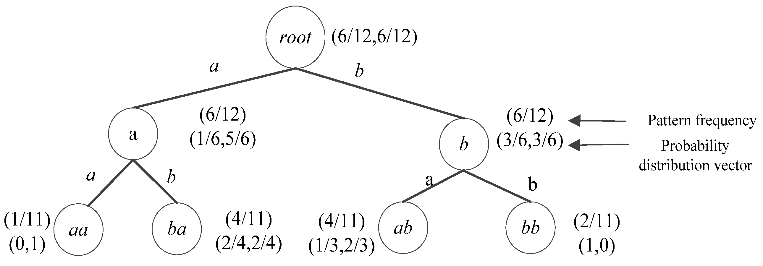
Figure 3 shows the wPST model of the sequence s₁ in Figure 1. Compared to PST, each node in the figure stores the conditional probability distribution vector of the subsequent symbol as well as the frequency weight corresponding subsequence, and thus can better present the feature information of the sequence.

The representation of a TSP is a trend feature over a period of time, such as a rising, a stable or a falling subsequence. Moreover, a time series TS of length n can be treated as a plurality of subsequences of length m (m <<= n); each subsequence has its own trend feature as well as the overall trend features of the original sequence. Therefore, the pattern features between different subsequences are closely related to the temporal trend of the sequence. For these reasons, this paper gives the definition of the hydrological time series anomaly subsequence and time series pattern anomalies based on the physical mechanism as below.

Definition 1.

Time series anomalous subsequence.

Given a time series TS, the event sequence set is Σ, the subsequence s, and the subsequent events σ of s (σ = suffix(s) & σ∈Σ). Let Pr_min and MinCt represent the predefined minimum occurrence probability and minimum occurrence number for the conditional occurrence probability of σ under the condition of s, respectively. If the conditional occurrence probability of σ under the condition of s is satisfied:

(1)

Pr (σ|s) < Pr_min and

(2)

occ_num(σ) ≤ MinCt,

then, it can define sσ to be an anomalous subsequence on time series TS.

As it can be seen from Definition (1), for a given time series TS, the smaller the probability of sσ occurring under the condition of s occurring, the higher the anomaly probability of sσ is. Therefore, the top k subsequences with the smallest occurrence probability (or occurrence number) are the top_k anomaly subsequences.

Definition 2.

Time series anomaly pattern.

The time series pattern anomaly is a pattern consisting of one or a series of consecutive anomalous subsequences within a given time series.

3.2. TFSAX_wPST Algorithm

3.2.1. TFSAX Representation

TFSAX is our previous work to extend the SAX representation. TFSAX employs the sequence mean feature and trend feature to represent the time series, and thus overcomes the shortcomings of SAX that only uses the mean values to describe the original time series. It can be obtained as follows:

Step 1: Normalization. Transform the original time series TS into the normalized time series TS′ with a mean of 0 and standard deviation of 1.

Step 2: Dimensionality reduction. Use the PAA (Piecewise Aggregate Approximation) approach [43] to divide time series TS′ into w equal-sized segments, then extract the mean feature and trend feature of each segment.

Step 3: Discretization. According to the breakpoints lookup table, choose alphabet cardinality, obtain the Trend Feature Symbolic Representation of the original time series and discretize TS′ into symbols, denoted by TS.

For more detailed information about TFSAX, please refer to our previous research work [23].

3.2.2. wPST Construction

The construction of wPST starts from a subsequence with a single element. It first initializes an empty wPST containing only one root node, and then iterates through all possible subsequences, with the length varying from 1 to L. For each to be checked subsequence s, its occurrence time should be greater than MinCt; then, continue to search the subsequent symbol σ (σ∈Σ) of s and count the occurrence times of sσ and σs to determine whether σ needs to be constructed in wPST; otherwise, discriminate all the subsequences, beginning with s, as being pattern anomalies, and stops searching.

To improve the algorithm’s efficiency, this approach uses the hash map data structure at each level to search and update the information of each node before and after a segment in the sequential database. For example, assume that we are at level 2 and the alphabet is {a, b}. Then, without pruning, the hash.keys at level 2 are all the possible 2 combinations of the alphabet:{aa, ab, ba, bb}. These combinations are lexicographically ordered, and the orders are stored at hash.values. Thus, the hash.values are {0, 1, 2, 3}. Now, the hash.key, hash.value combination is used as an index to the arrays A_before and A_after. Moreover, The arrays’ size is the size of the alphabet, and the value of each element of A_before is the current count of σs′, where s′ is the element of hash.keys and σ is a character in the alphabet. Similarly, A_after will store the count of s′σ. Thus, we can update all the counts at each level of the tree after one scan. After a level of the wPST is constructed, the current hash map is destroyed and a new hash map for the next level is initialized. For example, assuming that we have a sequential database consisting of one sequence {abba}, in one scan we can update the counts of ab→ b, a← bb, bb→ a and b← ba. The formal description of constructing wPST is shown in Algorithm 1.

Algorithm 1wPST construction. Build_wPST(S,H)

Input:   Sequence S, Maximum depth H

Output:   wPST T

1.   Initialize: T←  root; k = 0;

2.     k = 1, S1← {σ |σ∈Σ ∧ occ_count(σ) > 0}

3.     HM1←  HASHMAP(S1)

4.   While  k≤ H Do

5.   Foreach  (s′∈Sk)

6.      Abefore[|Σ|], Aafter[|Σ|]←0;

7.   For i = 1 to len(s) –k + 1

8.    ForEach (s[i,i + k−1] ∈ S)

9.      If  s[i,i + k−1] ∈ HMk.keys then

10.       Update(occ_times(s[i,i + k−1]));

11.    ForEach(σ∈Σ | |σ′∈Σ)

12.      If (s[i + k] =σ)  then  Update(Aafter(s[i + k]));

13.      If (s[i−1] =σ′)  then  Update(Abefore(s[i−1]));

14.    ForEach  (s′∈ Sk)

15.      T.Add(represent(u, s′));

16.      w(represent(u, s′)) = occ_times(s′)/(len(S)-k);

17.    ForEach  (σ∈Σ)

18.     compute  Pr(σ|s′) using Aafter;

19.     smooth  Pr(σ|s′);

20.     Mine_candidate_Anomaly (T, MinCt, Prmin);

21.   HMk + 1←  HASHMAP(Sk + 1);

22.   Return T

3.2.3. Candidate Anomalies Pattern Set Generation

Theoretically, the number of entries in the hash map on the Lth level of wPST is |Σ|^{L − 1} without pruning while wPST is constructed. Therefore, the total complexity of this implementation is O(NmL) + O(L × |Σ|^{L − 1}) [29]. Thus, we can prune the wPST by using Pr_min or MinCt, which only increases the number of nodes exponentially at first a few levels and then decreases and converges to some constant C. However, using the Pr_min or MinCt to perform the pruning operation during the wPST construction process may result in the loss of the anomalous subsequence. In order to solve the above problem, this paper proposes a strategy to put the sequence corresponding to the node whose occurrence number is less than MinCt or occurrence probability is less than Pr_min into the candidate pattern anomalies set, and then analyzes and mines the candidate set to obtain pattern anomalies that meets the user’s requirements.

During the wPST construction process, each node of the wPST stores the occurrence number of the string traversing from the root to this node, the occurrence probability of the node and the probability vector of the subsequent nodes. Hence, it only needs to analyze the node to determine if the sequence is a pattern anomaly or not during the wPST tree construction process; that is, if the sequence whose occurrence number is less than MinCt or the occurrence probability is less than Pr_min, then it puts the node corresponding to the sequence and all its descendant nodes into the candidate pattern anomalies set. The formal description of the candidate anomaly mining algorithm Mine_Candidate_ Anomaly is shown in Algorithm 2.

Algorithm 2 Candidate anomaly pattern mining. Mine_Candidate_Anomaly (wPST T, int MinCt, real Prmin)

Input:   wPST T, MinCt, Prmin

Output:  candidate pattern anomaly set cpas

1.   Initialize: cpas←∅

2.   ForEach represent(u,X) ∈T

3.     occ_times(u).Cal(); Pr (suffix(u)). Cal ();

4.     If (occ_times(u) < MinCt || Pr (u) < Prmin)

5.      caps.Add(represent(u,X));

6.      caps.Add(descendants (represent(u,X)));

7.      T.Prune(represent(u,X));

8.      T.Prune(descendants (represent(u,X)));

9.   Return caps

3.2.4. Pattern Anomalies Verification

Generally speaking, pattern anomalies have a higher probability coming from the candidate pattern anomalies set caps. However, there may be some special pattern anomalies that are not in the cpas; in addition, the cpas may also have partially redundant pattern anomalies. Hence, it is necessary to mine and analyze the cpas to obtain the pattern anomalies. The pattern anomalies mining mainly include:

(1) Pattern filtering: for pattern s₁ corresponding to node u and pattern s₂ corresponding to node v in the cpas, if pattern s₂ is a substring of the pattern s₁, add pattern s₁ to the pattern anomalies set pas.

(2) Pattern merging: for pattern s₁ corresponding to node u and pattern s₂ corresponding to node v in the cpas, if pattern s₁ and pattern s₂ have the longest common substring s₃; furthermore, s₃ is the true suffix of pattern s₁ and pattern s_2, then merge pattern s₁; (s₂-s₃) becomes the new pattern s′ and is added to the pattern anomalies set pas; else add s₃ to pas, where ′-′ in (s₂-s₃) means deleting pattern s₃ from s₂.

(3) Pattern expanding: for each pattern σ_is_i corresponding to node u_i (1 ≤ i ≤ |Σ|) and its parents node u in wPST, if pattern sσ corresponding to node u does not include in caps but all σ_is_i is included in caps, prune the parent node u corresponding to pattern sσ from wPST and add sσ to the pattern anomalies set pas.

(4) Pattern verifying: for each pattern sσ in cpas, if there exists an alphabet σ′∈Σ, make the occurrence number of sσ be equal to the occurrence number of sσσ′; that is, the probability that the event σ′ occurs after the event sσ is 1. Although the probability of event sσ is lower than MinCt, the occurrence of sσ represents the occurrence of a high confidence event sσσ′. Therefore, sσ cannot be simply treated as a pattern anomaly and should be deeply verified and analyzed.

(5) Pattern sorting: the probability of sequences corresponding to nodes in different levels of wPST is different. Generally, if the symbol sequence has the same occurrence number, the closer a node is to the root, the higher the probability it is to be an anomalous pattern. Thus, for pattern s₁ corresponding to node u₁ and pattern s₂ corresponding to node u₂ in the pas, if the occurrence number of s₁ equals the occurrence number of s₂ and the node u₁ is closer to root than u₂, it seems that s₁ has a higher probability to be an anomalous pattern than s₂. Therefore, the top-k anomalous patterns can be gained by using this rule to sort the patterns in pas.

The formal description of the pattern anomalies mining process is shown in Algorithm 3.

Algorithm 3 Anomalies Pattern Mining. Mine_Anomaly (CAPS caps)

Input:  candidate pattern anomaly set caps

Output:  pattern anomaly set aps

1.  Initialize: aps←∅

2.     Pattern_Filter(caps);

3.     Pattern_Merge(caps);

4.     Pattern_Extend(caps);

5.     Pattern_Valid (aps);

6.     Pattern_Sort(aps);

7.  Return aps

3.3. Algorithm Analysis

TFSAX_wPST can be divided into four parts: time series symbolization TFSAX, wPST construction, candidate pattern anomalies generation and pattern anomalies verification. For TFSAX, it has been proven to have a slightly more time complexity than SAX, but can achieve better symbolization. For the second part, it prunes the wPST by using Pr_min or MinCt, thus the number of nodes only increases exponentially at first a few levels and then decreases and converges to some constant C [29]. Therefore, the total cost of constructing the wPST is approximately equal to O(NmL) + O(L × |Σ|^α) + O(LC), where N is the total length of S, m is the average length of the sequence of S, α is a fixed integer, which depends upon the pruning parameters (usually less than 4), and C is a constant. Since the probability of pattern anomalies is small, the number of nodes included in the candidate pattern anomalies set is far less than |Σ|^{L − 1}. Therefore, the time complexity required for candidate pattern anomalies generation and pattern anomalies mining will be much lower than that of wPST construction. Hence, the time complexity of TFSAX_wPST is mainly concentrated on TFSAX representation and wPST construction. Theoretically, the performance and efficiency of our algorithm are effectively improved compared to PST-based methods.

4. Case Studies

In this section, we conduct a set of experiments to show the accuracy and feasibility of our new approach. Here we choose different datasets (the NWIS dataset and Poyang Lake dataset) for experiments to prove the generality of our model.

4.1. NWIS Dataset

4.1.1. Research Area

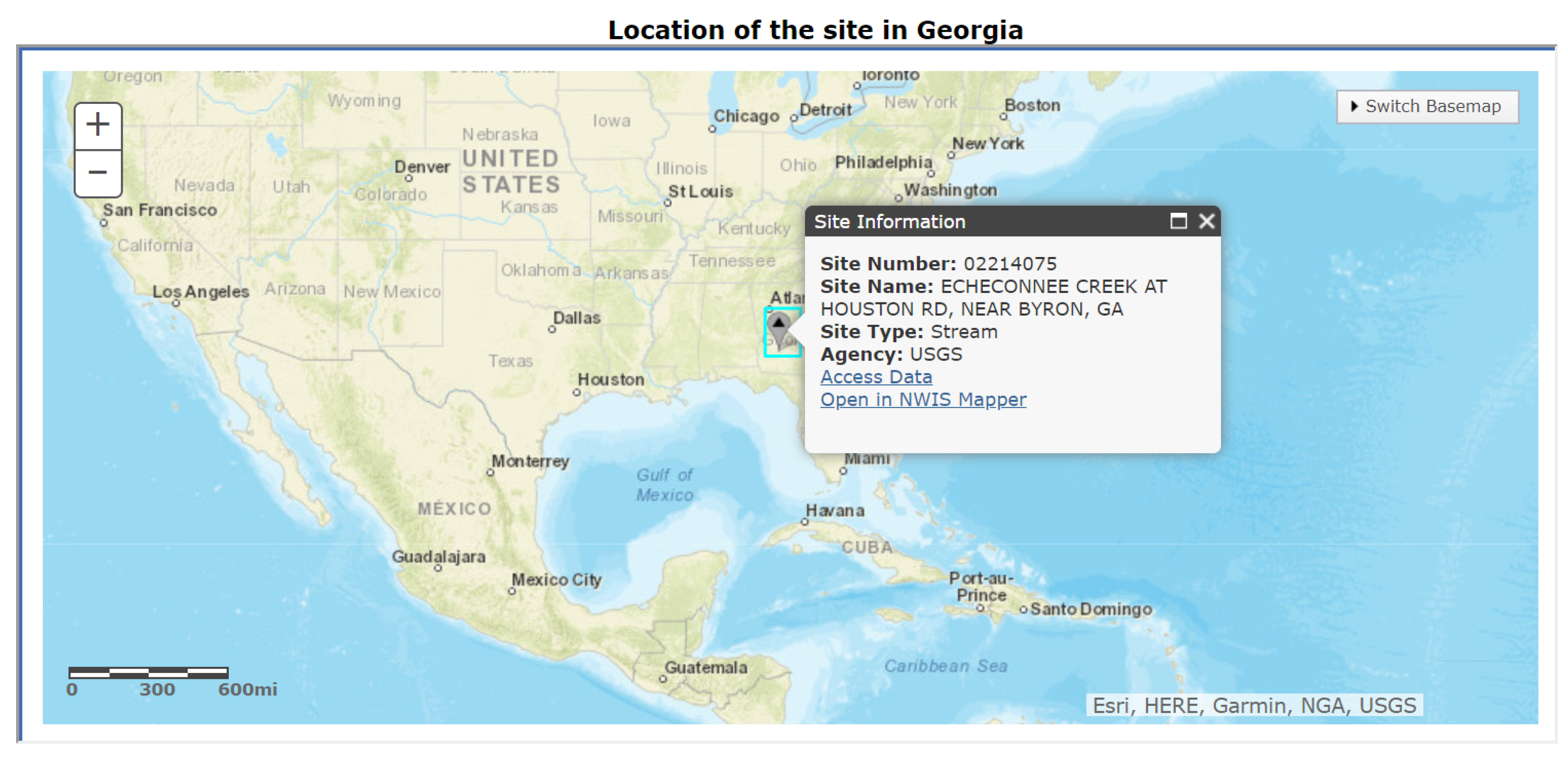
Echeconnee Creek (site number 02214075, location at 32°41’30.76” N, 83°42’03.5” E) is an important water level and flow control station in Peach County, Georgia. It is 9.1 miles from the confluence with the Ocmulgee River, 4.4 miles northwest of Byron, GA, and its basin has an area of 228 square miles (Figure 4). This station is a typical hydrological station in the southern United States. Every year from July to October, the water level and discharge gradually decrease due to the influence of the Atlantic monsoon and will fall to the lowest value in September or October. With the increase of precipitation from November to June of the following year, the water level and discharge begin to rise and will reach the highest level from January to February. According to historical data, its monthly mean water level varies from 6.4 feet (September) to 9.3 feet (February) and its monthly mean discharge varies from 76 ft³/s (October) to 452 ft³/s (February).

Therefore, we used hourly water level, discharge and rainfall from 15 November 2010 to 15 November 2013 provided by the NWIS, USGS (NWIS: https://waterdata.usgs.gov/nwis/inventory/?site_no=02214075&agency_cd=USGS&amp), to verify the feasibility and effectiveness of this algorithm. The original water level data is shown in Figure 5. It should be mentioned that we used data quality control methods in the literature [15] and the point outlier detection method in the literature [13] to perform data quality control and point outlier detection on the original data set, so as to provide high-quality data for pattern anomalies detection.

4.1.2. TFSAX Representation

As can be seen from Figure 5, the water level data of Station 02214075 is smooth overall, but there are still some local “extreme” patterns that are obviously inconsistent with other patterns. In order to discover those “interesting” information in the series, we first use TFSAX to transform hydrological time series into symbolic sequence representation. In this experiment, we discretize the daily monitoring data (including 24 monitoring records with an interval of 1 h) into a mean symbol and a trend feature symbol representation. Therefore, the experimental time series will be divided into 1096 sequence segments (the total number of days from 15 November 2010 to 15 November 2013); that is, w = 1096. According to the TFSAX, the mean and trend feature of the given time series from 15 November 2010 to 15 November 2013 can be represented by 5 and 7 symbols. That means the number of mean symbols is α = 5, and the number of trend feature symbols is α′ = 7. The character set represented by the mean and trend feature and their corresponding physical meanings are shown in

Table 1. The character sets and their meanings for the mean feature.

Symbol	Meaning (Water Level)
A	5.46 ft–7.45 ft
B	7.46 ft–9.43 ft
C	9.46 ft–10.39 ft
D	10.48 ft–13.44 ft
E	13.48 ft−16.56 ft

and

Table 2. The character sets and their meanings for the trend feature.

Symbol	Trend Feature	Meaning
a	(−90°–−45°)	water level drops sharply
b	(−90°–−30°)	water level drops rapidly
c	(−30°–−5°)	water level drops slowly
d	(−5°–5°)	water level remains stable
e	(5°–30°)	water level rises slowly
f	(30°–45°)	water level rises rapidly
g	(45°–90°)	water level rises sharply

.

After TFSAX symbolic representation, the original water level time series containing 1096 × 24 records will be symbolized into a symbol sequence containing 1096 symbols. The TFSAX representation of the water level time series is shown in

Table 3. The TFSAX representation of the daily mean water level of station 02214075.

Symbol	Frequency	Symbol	Frequency	Symbol	Frequency	Symbol	Frequency	Symbol	Frequency
Eb	1	Cc	3	Ea	5	Bf	11	Bd	33
Ee	1	Cf	3	Dc	5	Af	12	Be	37
Ec	1	Eg	3	Df	6	Bb	13	Ae	103
Ab	2	Ag	4	Ba	6	Dg	13	Bc	125
Ef	2	Db	4	Ca	9	Da	7	Ac	149
De	3	Cb	4	Cg	9	Bg	8	Ad	495

.

4.1.3. wPST Construction

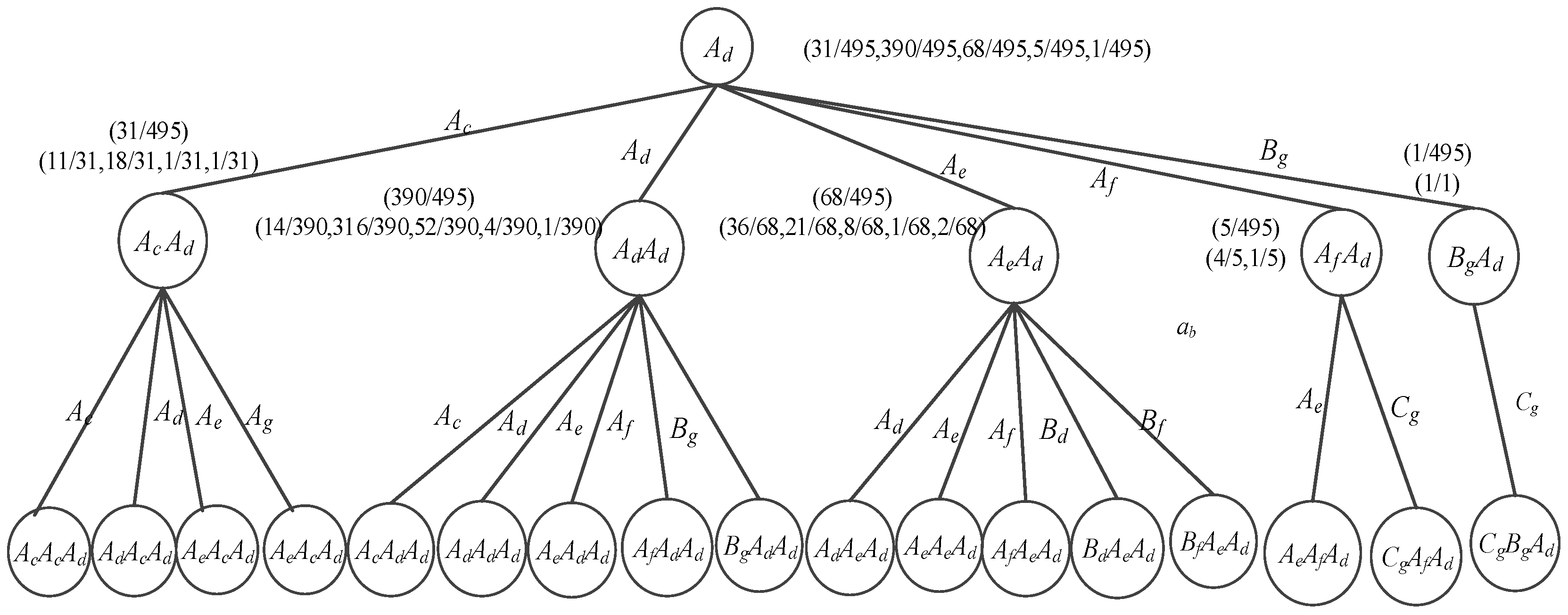
As shown in Table 3, we can find some pattern anomalies. For example, pattern E_b means the water level is in state E (high water level between 13.48 and 16.56 feet) and the trend feature is in state b (the water level drops rapidly, and the trend feature angle is −45°–30°) is a rare pattern in the time series. It will be added to the candidate pattern anomaly set according to TFSAX_wPST. In order to analyze the symbolized sequence, we used the wPST construction algorithm Build_wPST to construct the wPST for the sequences shown in Table 3. For the convenience of description, it uses A_d with the constraint of the depth of tree L ≤ 3 to illustrate the construction of wPST. The constructed wPST is shown in Figure 6.

4.1.4. Detection Results and Analysis

From Figure 6, it can be inferred that the normal subsequent stages of state A_d should be A_c, A_d and A_e. Hence, it may indicate an anomalous event occurred if state A_f or B_g appears right after state A_d. Here we use the algorithm Mine_Candidate_Anomaly and Mine_Anomaly to detect those patterns that meet the anomaly pattern definition in Definition (2).

In this experiment, we set parameters Pr_min = 0.01 and MinCt = 5. When wPST is constructed, any node whose occurrence probability is less than Pr_min or occurrence number is less than MinCt will be pruned from wPST. Moreover, the sequences corresponding to those nodes and all of its descendant nodes will be put into the candidate pattern anomalies set caps. For example, the node A_fA_d and all its descendant nodes will be pruned from the wPST shown in Figure 6, and all the sequences that contain patterns A_dA_f (e.g., A_dA_dA_f) will be put into the caps.

After caps is generated, we will validate and analyze the patterns in it to determine the final pattern anomalies. Take A_dB_g for instance: we checked and analyzed the original data shown in Figure 5 and find that the pattern A_dB_gC_g corresponds to the anomalous rain event from 15 August 2013 to 17 August 2013 in the Echeconnee Creek basin. On August 15, 16 and 17, the precipitation of this station was 1.41 in, 0.98 in and 1.45 in, respectively. As a result, the water level sharply rose 2.22 ft, 2.79 ft, 1.27 ft and 1.14 ft on 15 August–18 August, and the water level state represented by TFSAX changed drastically from A_d to B_g and then to C_g. Our method can quickly and accurately detect the pattern corresponding to this time series as an anomalous pattern. Similarly, the algorithm can also detect pattern anomalies, such as A_cA_e, A_cA_g, A_eB_d and A_fB_g, in a given time series.

The pattern anomalies detected by TFSAX_wPST on the Echeconnee Creek water level time series data set are shown in

Table 4. Anomalous patterns detected by the algorithm and event descriptions.

Pattern	Subsequence	Corresponding Event Description
BgCcBa	1 Dec 2010–3 Dec 2010	Daily water level is +1.88, −0.3, −1.19 feet, respectively.
BgDeDfDgEfEaDaCb	2 Feb 2011–9 Feb 2011	Daily water level is +1.68, +0.24, +1.33/2, +1.53, + 1.39/2, −1.53, −2.42, −0.8 feet, respectively.
BfCgDeCaBc	9 Mar 2011–12 Mar 2011	Daily water level is +2.13, +0.36, −2.35, −0.53 feet, respectively.
CgDgDbDcDfDbDaBbBcBgCfCa	27 Mar 2011–7 Apr 2011	Daily water level is +3.38, +1.6, −0.86, −0.31, + 0.9, −0.65, −1.74, −0.7, −0.39, +1.09, +0.61, −1.25 feet, respectively.
BgBcBb	23 Sep 2011–25 Sep 2011	Daily water level is +2.34/2, −0.51, −0.72 feet, respectively.
AgBg	21 Jan 2012–22 Jan 2012 2012.1.21–1.22	Daily water level is +1.3, +1.1 feet, respectively.
AfCgDfDaBcBb	18 Feb 2012–23 Feb 2012	Daily water level is +0.67, +2.67, +0.79, −2.1, −0.99 feet, respectively.
BfBgBaBc	26 Dec 2012–28 Dec 2012	Daily water level is +0.65, +1.49, −1.55 feet, respectively.
AgCgCaBaCgDgEeEcEaDaCaBc	7 Feb 2013–18 Feb 2013	Daily water level is +1.87, +1.78, −1.06, −1.14, +3.19, +3.44, +0.26, −0.32, −1.59, −2.04, −1.47, −0.57 feet, respectively.
BgDgEgEaDcDcEfEaDaCaBc	22 Feb 2013–2 Mar 2013	Daily water level is +1.14, +2.86, +1.85, −1.14, −0.2, +1.31, −1.24, −2.1, −1.15, −0.46 feet, respectively.
CgDgEaDaCb	24 Mar 2013–28Mar 2013	Daily water level is +3.25, 3.18/2, −1.62, −2.66, −0.88 feet, respectively.
BgDgDaBbBc BgDgEgDaDaBb	29 Apr 2013–9 May 2013	Daily water level is +2.04, +1.91, −1.98, −0.88, −0.31, +1.05, +2.55, +2.09/2, −1.31, −2.68, −0.9 feet, respectively.
CgEgDaBa	23 May 2013–26 May 2013	Daily water level is +4.21, +2.1/2, −3.97, −1.41 feet, respectively.
BgDcBfDgDfDbDaBcDgDfDa	3 Jun 2013–13 Jun 2013	Daily water level is +3.03, −0.24, +0.78, +2.17, +0.57, −0.8, −1.7, 0.35, +2.42, +0.6, −3.46 feet, respectively.
BfCfDaDeCaDgDaBa	3 Jul 2013–10 Jul 2013	Daily water level is +0.52, +0.46, −1.25, +0.25, −1.2, +1.61, −1.16, −1.13 feet, respectively.
CgDgDfDaBa	12 Jul 2013–16 Jul 2013	Daily water level is +1.97, +1.2, +0.57, −2.76, −1.11 feet, respectively.
AgBgCaBb	2013.7.31–8.3	Daily water level is +1.01, +2.43, −1.52, −0.92 feet, respectively.
BgCgDgDgEb	15 Aug 2013–19Aug 2013	Daily water level is +2.22, +2.79, +1.27, +1.14 feet, respectively.

. The analysis of the results and corresponding events verifies that our method can effectively detect anomalous patterns, and thus provides high-quality data and knowledge support for subsequent hydrological analysis and application.

4.2. Poyang Lake Data Set

4.2.1. Research Area

Poyang Lake (Figure 7), the largest freshwater lake in China, is an important reservoir lake and an important international wetland in the mainstream of the Yangtze River. It is located on the south bank of the middle reaches of the Yangtze River and north of Jiangxi Province. The catchment has a subtropical wet climate characterized by an annual mean precipitation of 1680 mm and an annual mean evaporation of 1200 mm. Poyang Lake receives water flows from five rivers: Ganjiang, Fuhe, Xinjiang, Raohe and Xiushui, and exchanges water with the Yangtze River. Lake storage and lake level variation is controlled by catchment discharges and interactions with the Yangtze River [44]. From April to June each year, the lake experiences large water level fluctuations in response to the catchment’s annual cycle of precipitation. From July to September, it is affected by the backflushing or backwatering of the Yangtze River to maintain high water levels. In the wet season (April to September), the water level rises and the lake coverage expands, covering an area of roughly 170 km from the north to the south and 17 km from the east to the west. The lake shrinks to little more than a river during the dry season (October to March), exposing extensive floodplains and wetland areas that support migrating waterfowls and a variety of invertebrate species [45].

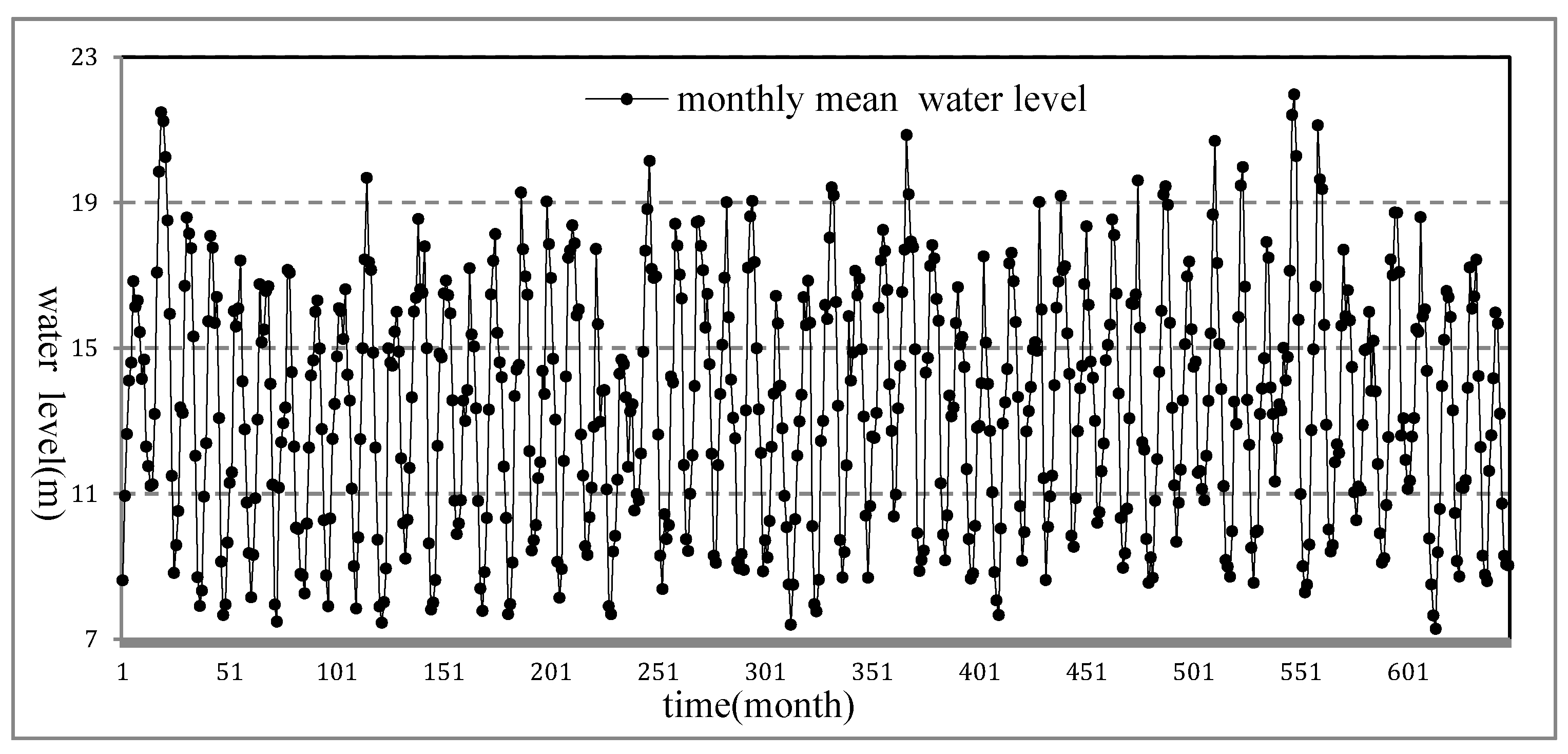
According to historical data, the multi-annual mean water level of Poyang Lake is 14.01 m; the monthly mean water level is highest in July (17.59 m) and lowest in January (10.52 m); and the highest water level appeared on 31 July 1998 (22.59 m), and the lowest appeared on 6 February 1963 (5.90 m). The Xingzi gauging station is the representative hydrological station of Poyang Lake and situated in the northern arm of the Lake at about 39 km from the Yangtze River. Typically, when the water level of Xingzi is below 11 m, it means that Poyang Lake has entered the dry season. Meanwhile, if the water level of Xingzi Station is above 19 m, it indicates that the water level of the Poyang Lake exceeds the warning line and is entering the flood season. The monthly mean lake water level at the Xingzi station from 1953 to 2009 is shown in Figure 8. We also used data quality control methods from the literature [15] and the point outlier detection method from the literature [13] to perform data quality control and point outlier detection on the original data set, so as to provide high-quality data for pattern anomalies detection.

4.2.2. TFSAX Representation

The monthly mean water level data of Xingzi Station is smooth overall in Figure 8, but there are still some local “extreme” patterns that are obviously inconsistent with other patterns. In order to discover those “interesting” patterns in this series, we first use TFSAX to transform the monthly mean water level data into a symbolic sequence representation.

In this experiment, we discretize the monthly statistics data (including 30 or 31 records with an interval of 1 day) into a mean symbol and a trend feature symbol representation. Therefore, the experimental time series will be divided into 684 sequence segments (the total number of month from January 1953 to December 2009); that is, w = 684. According to the TFSAX, both the mean and trend feature of the given time series from January 1953 to December 2009 would be represented by 5 symbols. That means the number of mean symbols is α = 5, and the number of trend feature symbols is α′ = 5. The character set represented by the mean and trend feature and their corresponding physical meanings are shown in

Table 5. The character sets and their meanings for the mean feature.

Symbol	Meaning (Water Level)
A	7.28 m–8 m
B	8.01 m–10.99 m
C	11.03 m–15 m
D	15.04 m–19 m
E	19.01 m−21.96 m

and

Table 6. The character sets and their meanings for the trend feature.

Symbol	Trend Feature	Meaning
a	(−90°–−30°)	water level drops rapidly
b	(−30°–−5°)	water level drops slowly
c	(−5°–5°)	water level remains stable
d	(5°–30°)	water level rises slowly
e	(30°–90°)	water level rises rapidly

.

After the TFSAX symbolic representation, the original water level time series containing 684 × 30 records will be symbolized into a symbol sequence containing 684 symbols. The TFSAX representation of the water level time series is shown in

Table 7. The TFSAX representation of the monthly average water level of the Xingzi station.

Symbol	Frequency	Symbol	Frequency	Symbol	Frequency	Symbol	Frequency
Aa	12	Bc	5	Cd	28	De	82
Ab	9	Bd	31	Ce	101	Ea	4
Ac	1	Be	37	Da	50	Eb	3
Ad	4	Ca	89	Db	31	Ed	4
Ba	73	Cb	24	Dc	9	Ee	16
Bb	29	Cc	12	Dd	30

.

4.2.3. wPST Construction

We can find some pattern anomalies in Table 7. For example, pattern B_a means when the water level is in state B (dry season, water level is 8–11 m), the trend feature is in state a (the water level drops rapidly, and the trend feature angle is −90°–−30°). It will be a rare pattern in the time series if the subsequent state of B_a is C (normal, water level is between 11 and 15 m) and the subsequent trend feature of B_a is e (water level rises rapidly, the trend feature angle is 30°–90°). It will be added to the candidate pattern anomaly set according to TFSAX_wPST.

In order to analyze the symbolized sequence, we used the algorithm Build_wPST to construct the wPST for the sequences shown in Table 7. For the convenience of description, it uses B_d under the constraint that the depth of tree L ≤ 3 to illustrate the construction of wPST. The constructed wPST is shown in Figure 9.

4.2.4. Detection Results and Analysis

From Figure 9, it can be inferred that state B_d (dry season, water level rises slowly) means the water level of Poyang Lake starts to rise slowly and its subsequent patterns is most likely to be B_d, B_e and C_e. So, it may indicate that an anomalous event occurred if states B_b or B_c appears right after state B_d. In order to detect those patterns that meet the anomaly pattern definition in Definition (2), we set parameters Pr_min = 0.02 and MinCt = 4.

When wPST is constructed, any node whose occurrence probability is less than Pr_min or occurrence number is less than MinCt will be pruned from wPST. Moreover, the sequences corresponding to those nodes and all of its descendant nodes will be put into the candidate pattern anomalies set caps. For example, the node B_cB_d and all its descendant nodes will be pruned from the wPST shown in Figure 9. Meanwhile, all the sequences that contain pattern B_dB_c (e.g., B_dB_cB_e) will be put into the caps.

After caps is generated, we will validate and analyze the patterns in it to determine the final pattern anomalies. Take pattern B_dC_eC_c for instance: we checked and analyzed the original data shown in Figure 8. It shows that the pattern B_dC_eC_c corresponds to the flood event from April to August 1974 in the Xingzi water level time series. Due to the influence of upper stream inflow from Ganjiang, Fuhe, Xinjiang, Raohe and Xiushui during the rainy season, the monthly mean water level of Xingzi Station soared from 10.13 m in April 1974 to 14.21 m in May, and dropped slightly in June to 14.05 m; then, in July, it rose to 18.41 m (the highest water level is 20.1 m). Our method can quickly and accurately detect the pattern corresponding to this time series as an anomalous pattern. Similarly, our algorithm can also detect other pattern anomalies, such as B_dB_eB_b corresponding to drought events at Poyang Lake from September 2006 to May 2007, and B_dB_cC_e corresponding to drought events at Poyang Lake from December 2007 to January 2008.

The pattern anomaly results detected by TFSAX_wPST on the Xingzi water level time series data set are shown in

Table 8. Anomalous patterns detected by the algorithm and event descriptions at the Xingzi station.

Pattern	Subsequence	Corresponding Event Description
DeEeEeEbEaDaDaCa	Mar 1954–Dec 1954	Extraordinary floods in the Yangtze River Basin, monthly mean water levels are 17.07, 19.84, 21.47, 21.23, 20.24, 18.5, 15.93, 11.48 m
AaAb	Dec 1958–Feb 1959	Extreme drought season, monthly mean water levels are 7.95, 7.48, 11.16 m
	Jan 1963–Oct 1963	Drought year, monthly mean water levels are 7.89, 7.45, 8.01, 8.94, 14.99, 14.59, 14.51, 15.45, 15.99, 14.9 m, highest water level occurred in September
	Dec 1971–Mar 1972	Extreme drought event, monthly mean water levels are 7.9, 7.68, 9.4, 9.83 m
	Dec 1979–Feb 1980	Extreme drought event, monthly mean water levels are 7.96, 7.76, 8.63, 12.4 m
AaAd	Jan 1965–Apr 1965	Extreme drought event, monthly mean water levels are 7.81, 8, 8.62, 12.31 m
	Jan 1968–Apr 1968	Extreme drought event, monthly mean water levels are 7.68, 7.9, 9.1, 13.68 m
	Dec 2007–Mar 2008	Extreme drought event, monthly mean water levels are 7.54, 7.72, 8.5, 8.62 m
DbDeEeEbDaCa	Jul 1980–Oct 1980	Flood events, monthly mean water levels are 18.03, 19.41, 19.19, 16.26 m
EeEaDaDcCa	Jul 1983–Oct 1983	Flood events, monthly mean water levels are 20.85, 19.22, 17.9, 17.77 m
CcEeDa	Jun 1968–Aug 1968	Flood events, monthly mean water levels are 14.53, 19.27, 17.71 m
CdCbCaCaCeCdBaBd	Jun 1972–Feb 1973	Drought year with a gentle overall trend, monthly mean water levels are 14.68, 14.55, 13.64, 11.73, 13.25, 13.45, 10.53, 10.98, 10.81 m
BaBbAbBe	Dec 1986–Feb 1987	Drought season, monthly mean water levels are 8.84, 8.06, 7.66, 8.34 m
DeEeEdEaDaBa	Jun 1998–Nov 1998	Extreme flood event, monthly mean water levels are 17.12, 21.4, 21.96, 20.17, 15.77, 10.98 m
DeEeEaEbDaCa	Jun 1999–Nov 1999	Flood events, monthly mean water levels are 16.69, 21.12, 19.63, 19.36, 15.63, 12.89 m
CaBaBaAbAbBe	Nov 2003–Mar 2004	Extreme drought event, monthly mean water levels are 8.5, 7.65, 7.28, 9.38 m
EeEd	Jul 1996–Oct 1996	Flood events monthly mean water levels are 19.46, 19.97 m
BdCeCcDe	Apr 1974–Jun 1974	No rainy season, monthly mean water levels are 10.13, 14.21, 14.05, 15.6 m
BaBaBbBcBaBdBeBbBe	Sep 2006–May 2007	Extreme drought year, monthly mean water levels are 10.72, 9.29, 9.05, 9.02, 8.06, 8.28, 10.6, 10.4, 10.98 m

. The analysis of the results and corresponding events verifies that our method can effectively detect anomalous patterns, and thus provides high-quality data and knowledge support for subsequent hydrological analysis and application.

4.3. Analysis and Discussion

In order to verify the accuracy and efficiency of our method, we conducted three sets of comparative experiments. We first compared the construction efficiency and detection accuracy of the wPST and PST models. Then we compared the detection result of our algorithm with other different algorithms. Lastly, we compared the time complexity of our algorithm with other hydrological time series pattern anomaly detection algorithms. The following performance metrics—True Positive Rate (TPR), True Negative Rate (TNR), False Positive Rate (FPR), False Negative Rate (FNR), Accuracy, Precision, Recall and F1-score and Area Under the Curve (AUC) [46]—were used to evaluate the different approaches.

4.3.1. Construction Algorithm Comparison

Here, we first compared the construction efficiency between the wPST model and the traditional PST model on the Poyang Lake daily water level dataset. In this experiment, the performance is measured by the negative log-likelihood of the normal patterns given the observation of the anomalous patterns. Specifically, we constructed both wPST and PST models from the experimental data with Markov orders 1, 2, 3, 4 and 5. For each wPST/PST model, we calculate the negative log-likelihood P (s|T) of the experiment sequence s based on the given wPST/PST model T. The larger the negative log-likelihood value is, the more dissimilar are the compared sequences. We expect the dissimilarity between the anomalous patterns and the normal patterns to grow as the memory order grows.

Our results are summarized in

Table 9. Comparison of the wPST vs. PST model.

Approach	Order	Numbers of Nodes	−Log-Likelihood
PST-based	1	10	−0.0152
	2	46	−0.0108
	5	138	−0.0068
wPST-based	1	10	−0.0152
	2	41	−0.0108
	5	84	−0.0068

. The empirical results indicate that the sizes of the wPST model are much smaller than that of the PST model as the order increases. For example, the 5th order PST model uses 138 states to characterize the experimental dataset, while the 5th order wPST model only uses 84 states. The negative log-likelihood is the same between a sequence given a wPST model and a PST model with the same order, since we eliminate nodes that have the same probabilities as their parent nodes when constructing the wPST models. Therefore, we prefer a wPST model over a PST model because it is purely data-driven, flexible, and takes less space.

Note that the PST models can be pruned to remove some low probability nodes [29]; which will lead to information loss. Unlike PST, our approach prunes the low probability nodes and puts the sequence corresponding to those nodes and all its descendant nodes into the candidate pattern anomalies set caps, which can improve the accuracy and reduce the false detection rate of our algorithm.

Table 10. Performances for wPST and PST.

Approach	MinCt	FNR (Miss Rate)	FPR (False Alarm)
PST-Based (order = 5)	1	25.2%	64.9%
	2	22.7%	42.5%
	5	14.3%	21.9%
	10	12.5%	37.6%
wPST-Based (order = 5)	1	12.6%	25.6%
	2	8.4%	10.9%
	5	2.3%	3.8%
	10	5.3%	8.4%

shows the confusion matrix obtained when adjusting the threshold MinCt. Based on the detection performances, the FPR for the wPST model on Poyang Lake dataset is 3.8% when MinCt = 5, which has the best tradeoff between FPR and TPR. As a comparison, the FPR for the PST model on Poyang Lake dataset is 21.9% when MinCt = 5, which has the best tradeoff between FPR and TPR. In addition, the miss rates for the PST and wPST models are 14.3% and 2.3%, respectively. The miss rates and false alarm rates are both relatively low for the wPST model. The detection results show that our proposed TFSAX_wPST algorithm is able to detect anomalies with a higher performance than that of the PST model.

4.3.2. Anomaly Detection Results Comparison

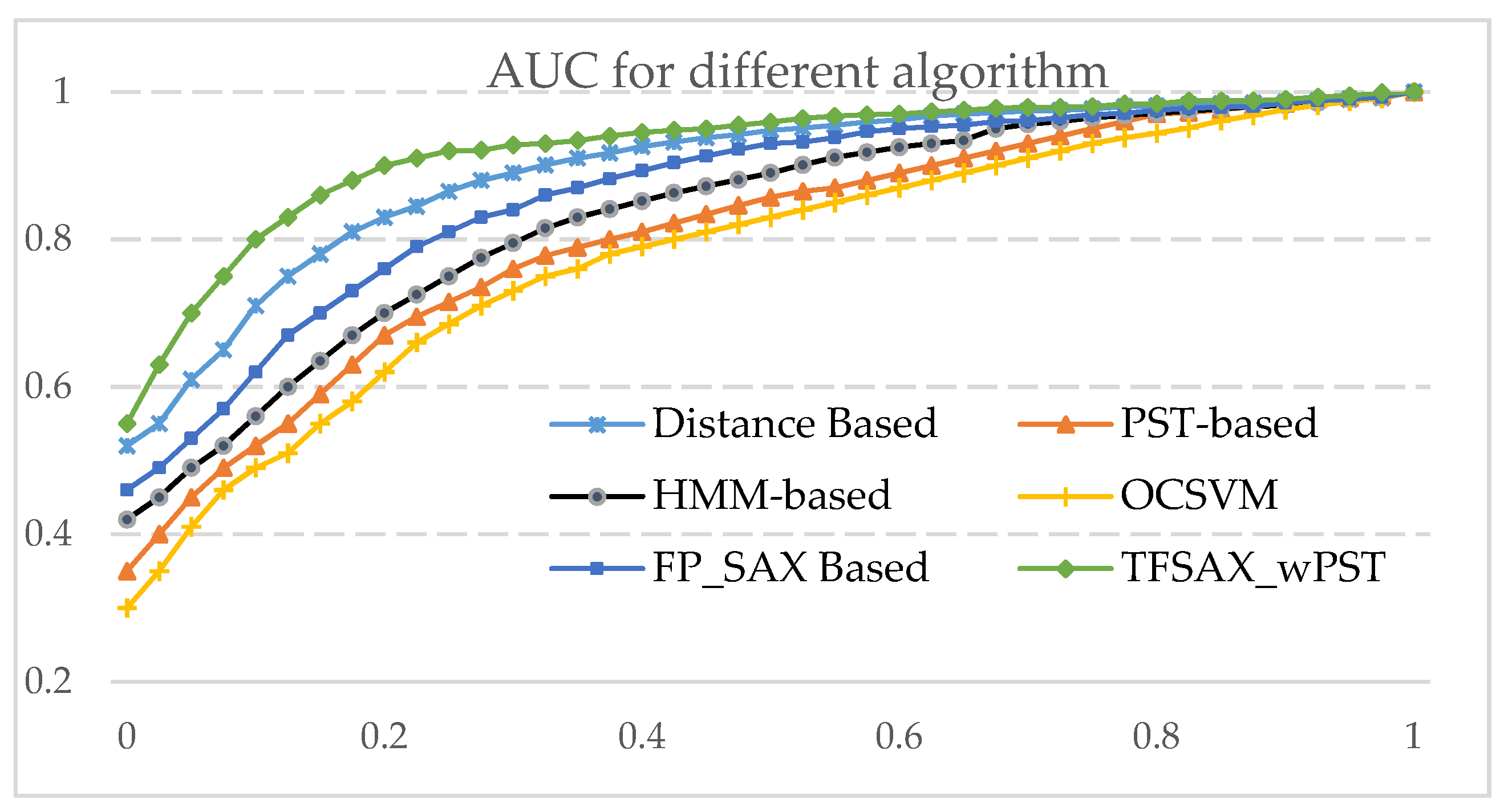
We compared the detection results of our algorithm with PST-based [41], HMM-based [31], OCSVM [47], FP_SAX-based [33], and Distance-based [34] algorithms on the same datasets. The detection results computed by the different algorithms on the Poyang Lake dataset are presented in

Table 11. Anomaly detection results for the Poyang Lake dataset.

	Algorithm	PST-based	HMM-based	OCSVM	FP_SAX-based	Distance-based	TFSAX_wPST
Metric
Accuracy		0.912	0.928	0.874	0.936	0.947	0.976
Precision		0.926	0.922	0.896	0.927	0.935	0.964
Recall		0.925	0.932	0.902	0.944	0.951	0.969
F1-score		0.926	0.927	0.918	0.935	0.943	0.966
AUC		0.924	0.931	0.915	0.938	0.949	0.971

. All results reported were averaged over 10 runs of both the representation learning and detection models.

The comparison results are displayed in the receiver operating characteristic (ROC) [48] curves shown in Figure 10. By convention, the ROC curve displays sensitivity (TPR) on the vertical axis against the complement of specificity (1 − specificity or FPR) on the horizontal axis. The ROC curve then demonstrates the characteristic reciprocal relationship between sensitivity and specificity, expressed as a tradeoff between the TPR and FPR. This configuration of the curve also facilitates calculation of the area beneath it as a summary index of the overall test performance. Therefore, the larger the area under the ROC curve, the better the performance of the technique is.

Figure 10 reveals the AUC obtained from the different algorithms. For experimental datasets, the AUC of the proposed algorithm are satisfactory and stable. These facts support the idea that our algorithm can effectively and accurately detect pattern anomalies and get better performances than that of OCSVM, HMM-based, PST-based, FP_SAX-based and Distance-based algorithms. This result is expected since the trend feature of the series is taken into account during the time series symbolization process TFSAX. Furthermore, we propose the improved probability suffix tree wPST to store the symbol sequence after TFSAX symbolization. Meanwhile, putting the symbol sequences pruned during the construction of wPST into caps rather than discarding them directly avoids information loss, which will improve the performance and efficiency of the algorithm.

4.3.3. Computational Complexity Comparison

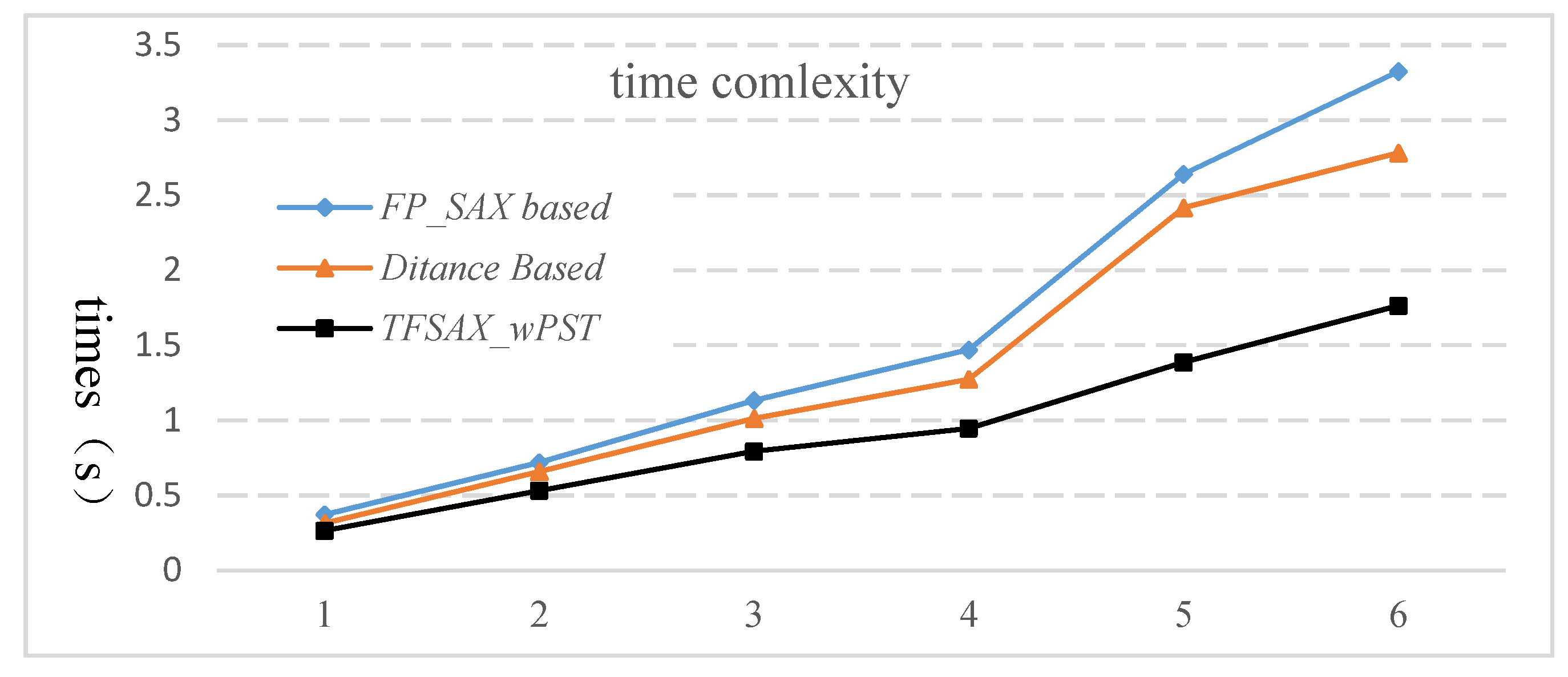
One important aspect of anomaly detection is efficiency. In the hydrological field, it is important to ensure that the pattern anomalies are computed in a short amount of time and with a minimum delay. In this section, we compare the execution time of the TFSAX_wPST, FP_SAX-based [33] and Distance-based [34] algorithms along with the increase of the length of sequences on the Poyang Lake daily water level. The comparison results are shown in

Table 12. The execution time of different approaches.

Num	Time	Sequence Lengths	Total Length	FP_SAX-based	Distance-based	TFSAX_wPST
1	Jul–Aug	62	3534	0.372 s	0.324 s	0.264 s
2	Jun–Aug	92	5244	0.719 s	0.708 s	0.532 s
3	Jun–Sep	122	6954	1.133 s	1.012 s	0.793 s
4	Jun–Oct	153	8721	1.471 s	1.274 s	0.946 s
5	May–Oct	184	10,488	2.641 s	2.416 s	1.387 s
6	Apr–Nov	244	13,908	3.325 s	2.782 s	1.764 s

and Figure 11.

From Table 12 and Figure 11, we can see that the execution time of TFSAX_wPST is obviously less than that of the FP_SAX-based method [33] and Distance-based method [34]. The main reason is that the FP_SAX-based method and Distance-based methods need to measure distance between patterns and result in relatively high time complexity. As discussed in Section 3.3, the time complexity of our approach is mainly concentrated on TFSAX representation and wPST construction. The time of TFSAX symbolization is slightly better than that of FP_SAX, but our algorithm does not need to calculate the distance between patterns, so the time complexity is greatly improved.

5. Conclusions

In this paper we have conducted in-depth research on time series anomaly patterns and their detection algorithms; particularly, a detailed analysis of the framework, advantages and disadvantages, as well as an improvement strategy for the wPST-based approach. Combining with the field of hydrology, we proposed an effective and accurate anomaly pattern detection approach TFSAX_wPST for hydrological time series. At present, it mainly uses a distance-based approach to detect anomalous patterns in hydrological time series; however, the time complexity to calculate the distance between each pattern is very high. In this work, we combined symbolization (TFSAX) of time series with the VMM model (wPST). Then, a new approach that is suitable for hydrological time series anomalous pattern detection is put forward, which makes the detection results accurate and efficient.

There are some parts that remain to be improved in the future. Firstly, in the candidate pattern anomalies mining step, the threshold Pr_min or MinCt to prune the wPST is based on the experience of previous experiments. In the future we should consider a more scientific way of evaluation, which achieves the optimal value of Pr_min or MinCt. Secondly, compared to the fixed-length segmentation method TFSAX, how to use variable-length segmentation to represent time series for hydrological feature extraction is a more meaningful and interesting question. Finally, our approach mainly analyzes univariate time series anomalous pattern detection; therefore, how to apply this approach to detect multivariate hydrological time series anomalous patterns is a topic for future research.

References

- Chen, L.; Wang, L. Recent advance in earth observation big data for hydrology. Big Earth Data 2018, 2, 86–107. [Google Scholar] [CrossRef] [Green Version]
- Guo, H.; Wang, L.; Chen, F.; Liang, D. Scientific big data and digital earth. Chin. Sci. Bull. 2014, 59, 5066–5073. [Google Scholar] [CrossRef]
- Azimi, S.; Moghaddam, M.A.; Monfared, S.A. Anomaly Detection and Reliability Analysis of Groundwater by Crude Monte Carlo and Importance Sampling Approaches. Water Resour. Manag. 2018, 32, 4447–4467. [Google Scholar] [CrossRef]
- Rougé, C.; Ge, Y.; Cai, X. Detecting gradual and abrupt changes in hydrological records. Adv. Water Resour. 2013, 53, 33–44. [Google Scholar] [CrossRef] [Green Version]
- Hawkins, D.M. Identification of Outliers; Chapman and Hall: London, UK, 1980. [Google Scholar]
- Chandala, V.; Banerjee, A.; Kumar, V. Anomaly Detection: A Survey. ACM Comput. Surv. CSUR 2009, 41, 1–58. [Google Scholar] [CrossRef]
- Gupta, M.; Gao, J.; Aggarwal, C.; Han, J. Outlier detection for temporal data. Synth. Lect. Data Min. Knowl. Discov. 2014, 5, 1–129. [Google Scholar] [CrossRef]
- USGS. Interagency Advisory Committee on Water Data. In Guidelines for Determining Flood Flow Frequency: Bulletin 17 B; U.S. Geological Survey, Office of Water Data Coordination: Reston, VA, USA, 1982. [Google Scholar]
- Stedinger, J.R.; Griffis, V.W. Flood frequency analysis in the united states: Time to update. J. Hydrol. Eng. 2008, 13, 199–204. [Google Scholar] [CrossRef] [Green Version]
- Chebana, F.; Daboniang, S.; Ouarda, T.B. Exploratory functional flood frequency analysis and outlier detection. Water Resour. Res. 2012, 48, 1–20. [Google Scholar] [CrossRef] [Green Version]
- Sarraf, A.P. Flood outlier detection using PCA and effect of how to deal with them in regional flood frequency analysis via L-moment method. Water Resour. 2015, 42, 448–459. [Google Scholar] [CrossRef]
- Amin, M.T.; Rizwan, M.; Alazba, A.A. Comparison of mixed distribution with EV1 and GEV components for analyzing hydrologic data containing outlier. Environ. Earth Sci. 2015, 73, 1369–1375. [Google Scholar] [CrossRef]
- Yu, Y.; Zhu, Y.; Li, S.; Wan, D. Time series outlier detection based on sliding window prediction. Math. Probl. Eng. 2014. [Google Scholar] [CrossRef]
- Ng, W.W.; Panu, U.S.; Lennox, W.C. Chaos based analytical techniques for daily extreme hydrological observations. J. Hydrol. 2007, 342, 17–41. [Google Scholar] [CrossRef]
- Zhao, Q.; Zhu, Y.; Wan, D.; Yu, Y.; Cheng, X. Research on the Data-Driven quality control method of hydrological time series data. Water 2018, 10, 1712. [Google Scholar] [CrossRef] [Green Version]
- Nyeko-Ogiramoi, P.; Willems, P.; Ngirane-Katashaya, G. Trend and variability in observed hydrometer- orological extremes in the Lake Victoria basin. J. Hydrol. 2013, 489, 56–73. [Google Scholar] [CrossRef]
- Wang, C.; Zhao, Z.; Gong, L.; Zhu, L.; Liu, Z.; Cheng, X. A distributed anomaly detection system for in-vehicle network using HTM. IEEE Access 2018, 6, 9091–9098. [Google Scholar] [CrossRef]
- Van Vlasselaer, V.; Bravo, C.; Caelen, O.; Eliassi-Rad, T.; Akoglu, L.; Snoeck, M.; Baesens, B. APATE: A novel approach for automated credit card transaction fraud detection using network-based extensions. Decis. Support Syst. 2015, 75, 38–48. [Google Scholar] [CrossRef] [Green Version]
- Golmohammadi, K.; Zaiane, O.R. Time series contextual anomaly detection for detecting market manipulation in stock market. In Proceedings of the International Conference on Data Science and Advanced Analytics (DSAA), Paris, France, 19–21 October 2015; pp. 1–10. [Google Scholar]
- Sultani, W.; Chen, C.; Shah, M. Real-world anomaly detection in surveillance videos. In Proceedings of the IEEE Conference on Computer Vision and Pattern Recognition, Salt Lake City, UT, USA, 18–22 June 2018; pp. 6479–6488. [Google Scholar]
- Keogh, E.; Lin, J.; Fu, A. HOT SAX: Efficiently Finding the Most Unusual Time Series Subsequence. In Proceedings of the IEEE International Conference on Data Mining, Houston, TX, USA, 27–30 November 2005; IEEE Computer Society: Washington, DC, USA, 2005; pp. 226–233. [Google Scholar]
- Candelieri, A. Clustering and support vector regression for water demand forecasting and anomaly detection. Water 2017, 9, 224. [Google Scholar] [CrossRef]
- Yu, Y.; Zhu, Y.; Wan, D.; Liu, H.; Zhao, Q. A Novel Symbolic Aggregate Approximation for Time Series. In Proceedings of the 13th International Conference on Ubiquitous Information Management and Communication, IMCOM 2019, Phuket, Thailand, 4–6 January 2019; Springer: Cham, Switzerland, 2019; pp. 805–822. [Google Scholar]
- Ding, Z.; Fei, M. An anomaly detection approach based on isolation forest algorithm for streaming data using sliding window. IFAC Proc. Vol. 2013, 46, 12–17. [Google Scholar] [CrossRef]
- Budalakoti, S.; Srivastava, A.N.; Otey, M.E. Anomaly detection and diagnosis algorithms for discrete symbol sequences with applications to airline safety. IEEE Trans. Syst. Man Cybern. Part C Appl. Rev. 2009, 39, 101–113. [Google Scholar] [CrossRef]
- Safin, A.M.; Burnaev, E. Conformal kernel expected similarity for anomaly detection in time-series data. Adv. Syst. Sci. Appl. 2017, 17, 22–33. [Google Scholar]
- Chandola, V.; Banerjee, A.; Kumar, V. Anomaly detection for discrete sequences: A survey. IEEE Trans. Knowl. Data Eng. 2010, 24, 823–839. [Google Scholar] [CrossRef]
- Keogh, E.; Lonardi, S.; Chiu, B.Y. Finding surprising patterns in a time series database in linear time and space. In Proceedings of the ACM SIGKDD International Conference on Knowledge Discovery and Data Mining, Edmonton, AB, Canada, 23–26 July 2002; pp. 550–556. [Google Scholar]
- Sun, P.; Chawla, S.; Arunasalam, B. Mining for Outliers in Sequential Databases. In Proceedings of the SIAM International Conference on Data Mining, Bethesda, MD, USA, 20–22 April 2006; 2006; pp. 94–105. [Google Scholar]
- Klerx, T.; Anderka, M.; Büning, H.K.; Priesterjahn, S. Model-based anomaly detection for discrete event systems. In Proceedings of the International Conference on Tools with Artificial Intelligence, Limassol, Cyprus, 10–12 November 2014; pp. 665–672. [Google Scholar]
- Zohrevand, Z.; Glasser, U.; Shahir, H.Y.; Tayebi, M.A.; Costanzo, R. Hidden Markov based anomaly detection for water supply systems. In Proceedings of the International Conference on Big Data, Washington, DC, USA, 5–8 December 2016; pp. 1551–1560. [Google Scholar]
- Pimentel MA, F.; Clifton, D.A.; Clifton, L.; Tarassenko, L. A review of novelty detection. Signal Process. 2014, 99, 215–490. [Google Scholar] [CrossRef]
- Wan, D.; Xiao, Y.; Zhang, P.; Feng, J.; Zhu, Y.; Liu, Q. Hydrological time series anomaly mining based on symbolization and distance measure. In Proceedings of the 2014 IEEE International Congress on Big Data, Beijing, China, 27 June–2 July 2014; pp. 339–346. [Google Scholar]
- Zhang, P.; Leung, H.; Xiao, Y.; Feng, J.; Wan, D.; Li, W.; Leung, H. A New Symbolization and Distance Measure Based Anomaly Mining Approach for Hydrological Time Series. Int. J. Web Serv. Res. 2016, 13, 26–45. [Google Scholar] [CrossRef] [Green Version]
- Wu, H.; Li, X.; Qian, H. Detection of Anomalies and Changes of Rainfall in theYellow River Basin, China, through Two Graphical Methods. Water 2018, 10, 15. [Google Scholar] [CrossRef] [Green Version]
- Ye, N. A markov chain model of temporal behavior for anomaly detection. In Proceedings of the 2000 IEEE Systems, Man, and Cybernetics Information Assurance and Security Workshop, West Point, NY, USA, 6–7 June 2000; Volume 166, p. 169. [Google Scholar]
- Ron, D.; Singer, Y.; Tishby, N. The power of amnesia: Learning probabilistic automata with variable memory length. Mach. Learn. 1996, 25, 117–149. [Google Scholar] [CrossRef] [Green Version]
- Bejerano, G.; Yona, G. Variations on probabilistic suffix trees: Statistical modeling and prediction of protein families. Bioinformatics 2001, 17, 23–43. [Google Scholar] [CrossRef]
- Yang, J.; Wang, W. CLUSEQ: Efficient and effective sequence clustering. In Proceedings of the 19th International Conference on Data Engineering, Bangalore, India, 5–8 March 2003; pp. 101–112. [Google Scholar]
- Kholidy, H.A.; Yousof, A.M.; Erradi, A.; Abdelwahed, S.; Ali, H.A. A Finite Context Intrusion Prediction Model for Cloud Systems with a Probabilistic Suffix Tree. In Proceedings of the 2014 European Modelling Symposium, Pisa, Italy, 21–23 October 2014; pp. 526–531. [Google Scholar]
- Li, Y.; Thomason, M.; Parker, L.E. Detecting time-related changes in Wireless Sensor Networks using symbol compression and Probabilistic Suffix Trees. In Proceedings of the 2010 IEEE/RSJ International Conference on Intelligent Robots and Systems, Taipei, China, 18–22 October 2010; pp. 2946–2951. [Google Scholar]
- Farahani, I.V.; Chien, A.; King, R.E.; Kay, M.G.; Klenz, B. Time Series Anomaly Detection from a Markov Chain Perspective. In Proceedings of the 2019 18th IEEE International Conference on Machine Learning and Applications (ICMLA), Boca Raton, FL, USA, 16–19 December 2019; pp. 1000–1007. [Google Scholar]
- Keogh, E.; Chakrabarti, K.; Pazzani, M.; Mehrotra, S. Dimensionality Reduction for Fast Similarity Search in Large Time Series Databases. Knowl. Inf. Syst. 2000, 3, 263–286. [Google Scholar] [CrossRef]
- Hu, Q.; Feng, S.; Guo, H.; Chen, G.; Jiang, T. Interactions of the Yangtze river flow and hydrologic processes of the Poyang Lake, China. J. Hydrol. 2007, 347, 90–100. [Google Scholar] [CrossRef]
- Li, X.; Zhang, Q.; Ye, X. Dry/wet conditions monitoring based on TRMM rainfall data and its reliability validation over Poyang Lake Basin, China. Water 2013, 5, 1848–1864. [Google Scholar] [CrossRef]
- Han, J.; Jian, P.; Micheline, K. Data Mining: Concepts and Techniques, 3rd ed.; Morgan Kaufmann Publishers Inc.: Burlington, MA, USA, 2011. [Google Scholar]
- Ghafoori, Z.; Erfani, S.M.; Rajasegarar, S.; Karunasekera, S.; Leckie, C.A. Anomaly Detection in Non-stationary Data: Ensemble based Self-Adaptive OCSVM. In Proceedings of the International Joint Conference on Neural Networks, Vancouver, BC, Canada, 25–29 July 2016. [Google Scholar]
- Fawcett, T. An introduction to ROC analysis. Pattern Recognit. Lett. 2006, 27, 861–874. [Google Scholar] [CrossRef]
Figure 1.
Probabilistic Suffix Tree (PST) representation for “abbabbabaaba”.
Figure 2.
Framework of the Trend Feature Symbolic Aggregate approximation and weighted PST approach (TFSAX_wPST).
Figure 3.
wPST representation for “abbabbabaaba”.
Figure 4.
Echeconnee Creek station and its location in Georgia, USA.
Figure 5.
Real-time water level data of Echeconnee Creek.
Figure 6.
wPST tree representations for event Ad.
Figure 7.
The Xingzi station and its location in the Poyang Lake and Yangtze River.
Figure 8.
Monthly mean water level at the Xingzi Station.
Figure 9.
wPST tree representations for event Bd.
Figure 10.
AUC for the different algorithms.
Figure 11.
A comparison of the runtime of different approaches.