Integrated Hydrologic and Hydrodynamic Models to Improve Flood Simulation Capability in the Data-Scarce Three Gorges Reservoir Region

Abstract

One-dimensional hydrodynamic modeling approaches are useful for flood simulations; however, most studies often neglect intermediate discharges due to difficulties in obtaining the associated data. Herein, we produced the XAJ-H1DM model by coupling the Xinanjiang (XAJ) model, without the Muskingum module, with a one-dimensional hydrodynamic (H1DM) model, using regionalization approaches to test their practicality. Another model, named H1DM-XAJ, was also produced by orderly calibrating the H1DM and XAJ models to achieve improved flood simulations in poorly gauged catchments. The flood simulation capabilities of the four models (including the single XAJ and H1DM models) were investigated and compared at a daily time scale in the Three Gorges Reservoir Region, China. The results show that the regionalization approaches can be successfully used in the application of the integrated hydrologic and hydrodynamic model in ungauged intermediate catchments. Further, the coupled models produced markedly improved estimates of peak discharge and runoff volume compared to the single models. Moreover, the ability of the coupled models to simulate the peak water level and hydrograph, which hydrological models lack, is significantly better than that of the single H1DM model. The framework presented can be applied in other data-scarce catchments worldwide for better understanding of the hydrodynamic processes.

1. Introduction

Floods are one of the most serious natural disasters associated with water, causing severe property damage and loss of life. To reduce the impact of flooding, operational flood simulation systems have been developed around the world [1]. The growing necessity of these operational systems has promoted the development of hydrodynamic models, which are commonly used in the existing systems [1,2]. With the rapid development of computational technologies, a large number of studies on hydrodynamic models for flood simulations and forecasting have been carried out over the past several decades [3,4,5,6,7,8,9,10,11,12,13].

Multi-model coupling integrates the selected model software to form a secondary processing integration process. The more thorough the secondary processing integration, the tighter the coupling simulation system integration. According to the ease of the secondary development in question, secondary processing integration can be divided into four categories: non-integrated, loosely coupled, tightly coupled, and fully integrated [14]. The non-integrated category refers to independent simulations running among various models and a final comprehensive analysis of the simulation results; loose coupling refers to the information transfer between each model, but the transmission process requires human participation to operate; and tight integration and full integration, with secondary development, refer to the fully automated operation of a coupled simulation system.

Satisfactory hydrodynamic modeling of many receiving water bodies is limited because in situ observations of river discharge are scarce or unavailable [15]. Integrated hydrologic and hydrodynamic modeling is widely used for river discharge modeling in ungauged or poorly gauged water bodies [16]. External coupling is the simplest and most common approach, in which discharge from the hydrologic model provides inputs for the hydrodynamic model [17,18]. External coupling overcomes the limitations of the hydrologic model in describing the dynamic processes of reservoirs [18]. This approach is widely used to quantify hydrodynamic characteristics [18,19,20,21,22,23,24] and the impacts of climate change and human activities (e.g., land-use change) on currents and water quality [15,16,25] in rivers, estuaries, lakes, and reservoirs.

However, the simulation of runoff in ungauged basins is difficult (e.g., determining a suitable set of parameters without calibration) in hydrology [26,27,28,29], and improving the accuracy of hydrologic models is key for comparative research in integrated modeling [15]. Regionalization approaches for runoff simulation in ungauged basins have respective advantages and limitations [27,30,31,32,33,34,35]. Among these approaches, parameter replacement is one of the most common methods used in hydrologic modeling in ungauged basins—the parameters from basins with calibrated data are transposed to hydrologically similar ungauged or poorly gauged basins [35,36,37,38]. The hydrological similarity is key for parameter replacement. In general, parameter replacement based on climatic and/or physiographic similarity has performed better than (or has given comparable results to) other approaches [35,38]. However, most studies are aimed at small basins that contain the initial section of the river, which have similar or adjacent basins nearby, but there are few studies on intermediate runoff prediction. Therefore, questions such as (i) whether the regionalization approaches can be successfully used in the application of the integrated hydrologic and hydrodynamic model, and (ii) how the performance of the coupled models can be improved in ungauged intermediate catchments remained unanswered. Unfortunately, there has been little guidance in the modeling literature on these two questions.

The first objective of this paper is, therefore, to assess the flood simulation capability of an integrated hydrologic and hydrodynamic model using regionalization approaches. The Xinanjiang model, which is the most popular conceptual rainfall-runoff model in China, has been extensively used for flood simulation and operational forecasting in gauged catchments since it was first developed in the 1970s. The flood events simulated by the Xinanjiang (XAJ) model are extremely sensitive to the parameters of the Muskingum runoff routing method [39]. In spite of its ease of implementation, this method is not theoretically strong. This method is very convenient, but relies too much on experience. Moreover, its parameters are purely empirical according to Zhao [40]. The preconditions of the Muskingum method are not always met, but alternative methods have not been well studied for data-scarce areas. Therefore, we initially use a more meaningful routing technique instead of the Muskingum method. A one-dimensional hydrodynamic approach based on the complete Saint-Venant equation is often used to simulate flood evolution [12,41,42,43]. This approach is advantageous because it accurately simulates the complete flow process of the natural river. In channels of river-type reservoirs, the one-dimensional hydrodynamic method should be used instead of the Muskingum method to simulate the progression of floods. In this paper, we propose a coupled model, called XAJ-H1DM, which couples the one-dimension hydrodynamic model (H1DM) with the Xinanjiang model (XAJ) without using the Muskingum module. Because the H1DM describes the complete fluid characteristics in the channel, we think it is more appropriate for channel flood simulation. A nested region containing interior stream gauging stations was selected as the study region. Merz and Blöschl [44] showed that strong regional similarities exist for nested catchments and better performance can be achieved by using the parameters transposed from nested neighbors. In this study, the model parameters for the exterior locations were regionalized by transposition from the interior catchments.

Second, we intend to address how to improve the flood simulation capability of the integrated hydrologic and hydrodynamic model for ungauged intermediate catchments. When the rainfall-runoff model is applied in a non-intermediate basin, where there is only one outlet in the entire basin, all runoff is generated by rainfall [27,45,46]. However, in intermediate basins, runoff is composed of input from the upstream channel flow and the intermediate rainfall runoff. The former usually accounts for a larger proportion of the total runoff. In the rainstorm season, the latter ratio cannot be ignored [47]. For unmeasured intermediate basins, runoff is usually simulated with nested sub-basins parameters or adjacent basins parameters [27]. However, in adjacent or similar watersheds, appropriate parameters may not always be available for transfer [36]. Hence, we think we start with a more valuable coupled method to avoid this dilemma. Usually, the rainfall-runoff model solves this problem by first evolving the upstream flow of the river to the downstream flow and then using the rainfall-runoff model to simulate the intermediate runoff [48]. In the first step, the method of evolution chosen is usually the Muskingum method. As mentioned above, the Muskingum method can be replaced by the H1DM method. Therefore, we improved the coupling method mentioned above (XAJ-H1DM) and further proposed a coupled model called H1DM-XAJ, which first simulated the flow from upstream to downstream using the H1DM model; then, the XAJ model was used to simulate the intermediate rainfall.

Our specific objectives are: (i) to assess the flood simulation capability of the XAJ model and the H1DM model respectively; (ii) to evaluate the performance of the integrated hydrologic and hydrodynamic model using parameter replacement from interior basins; and (iii) to compare two coupled models to determine which is more appropriate in an ungagged intermediate basin.

2. Materials and Methods

2.1. Study Area

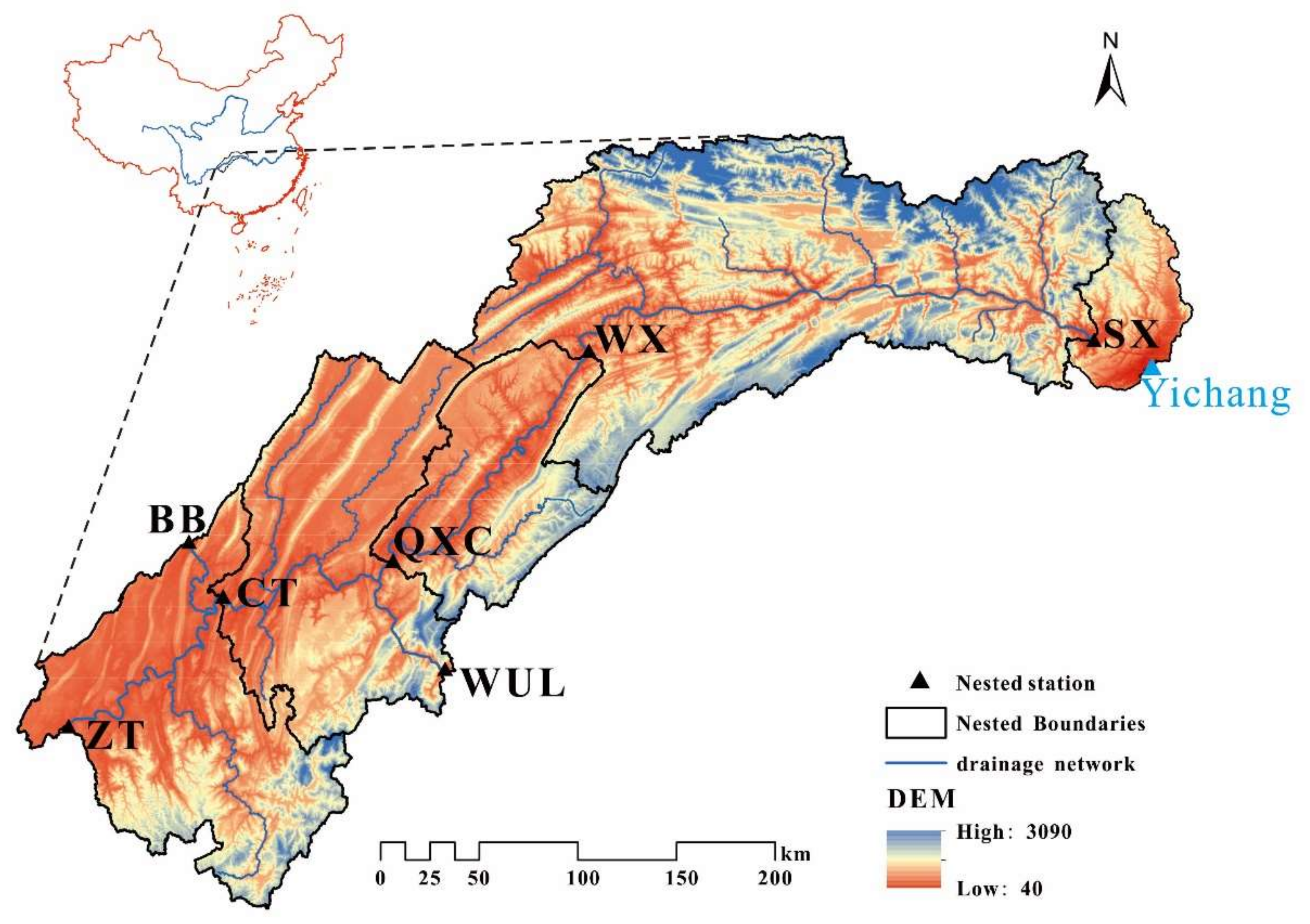
The Zhutuo-Three Gorges Dam area, located in the middle reaches of the Yangtze River, China, is chosen as our study area (Figure 1). The Three Gorges Reservoir (Figure 1, SX), a typical River type reservoir with a modified end, is located approximately 40 km west of Yichang City in Hubei Province, central China (Figure 1, 106°53′–109°43′ E, 28°60′–30°56′ N). It is one of the largest reservoirs in the Yangtze River basin, with a water surface area of 1084 km² and a storage capacity of 393 billion m³ at a normal water level (175 m, Wusong Elevation System). The length of the mainstream in the study area is approximately 760 km, and the reservoir surface width of the mainstream is generally 700–1700 m. The topography of the study area (Figure 1, 90 × 90 m, Digital Elevation Model) shows great variation, with the highest elevation (3090 m) in the northeast and the lowest elevation (40 m) in the northwest.

Figure 1 shows a schematic diagram of the ZT to Dam section of the Three Gorges Reservoir area. There are five hydrometric stations in study area, Zhutuo (ZT), Cuntan (CT), Qingxichang (QXC), Wanxian (WX), and Sanxia (SX), from upstream to downstream. The storage control stations of the Jialing River and Wujiang River, two major tributaries of the reservoir area, are the Beibei hydrometric station (BB) and the Wulong hydrometric station (WUL), respectively.

2.2. Dataset

The landscape characteristics of all catchments were derived from a DEM with a spatial resolution of 90 m (3’’) provided by Geospatial Data Cloud site, Computer Network Information Center, Chinese Academy of Sciences (http://www.gscloud.cn). Station observations of rainfall, discharge and E-601 pan evaporation data for these catchments were used to assess the performance of the Xinanjiang model and coupled models.

The river section data includes 368 sections from the ZT to the Three Gorges Dam, 30 sections from the BB to the Yangtze River mainstream, and 46 sections from the WUL Station to the Yangtze River mainstream. In addition, there are 12 tributaries with measured section data and a total of 144 sections.

2.3. Watershed Division

There are several hydrometric stations in the study area. According to the location distribution of key hydrometric stations in mainstream, the study area is divided into four sub-regions, namely ZT-CT, CT-QXC, QXC-WX, and WX-SX. The dividing line is determined according to the topography of the natural watershed. The areas of these four sub-regions are: 14,555 km², 15,086 km², 8611 km², 31,215 km². The area of the whole study area is 69,467 km². Each sub-region contains several rainfall sites, evaporation sites, and several sub-catchments. Sub-catchments are extracted based on terrain using the ArcGIS tool.

2.4. The Xinanjiang Model

The Xinanjiang model was first used to predict the storage of the Xinanjiang Reservoir and later became a general-purpose rainfall-runoff model. Its main feature is the formation of runoff as a dependent variable of the storage recharge, that is, no runoff is generated before the soil water content in the aeration zone reaches the field water holding capacity. Thereafter, the runoff is equal to the excess rainfall without further loss. The Xinanjiang model, with four runoff components, has been widely used in humid or semi-humid regions in China, as well as in many other countries. The overall structure of the Xinanjiang model is shown in Figure 2.

For each sub-catchment, the outflow is calculated by four major modules:

• Evapotranspiration module: the three-layer evapotranspiration mode—that is, the total evaporation is composed of three parts, namely, surface evaporation, shallow evaporation, and deep evaporation.
• Runoff generation module: runoff generation under saturated conditions—that is, the precipitation does not produce flow before the field water capacity is satisfied, and all precipitation is absorbed by the soil. After the precipitation meets the field water holding capacity, all precipitation (excluding the evaporation in the same period) produces flow.
• Runoff separation module: the division of the three water sources—that is, according to the free water capacity distribution curve, the total production flow is divided into the surface runoff, soil middle flow, and underground runoff.
• Runoff routing module: this module is divided into the river network confluence and the river channel confluence. The river network confluence is runoff that flows directly into the sub-catchment outlet; the river confluence is the runoff at the sub-catchment outlet that uses the Muskingum method to evolve the basin exit.

2.5. The One-Dimensional (1-D) Hydrodynamic Model

The 1-D hydrodynamic model (H1DM) was used to simulate the hydrodynamic processes of the study area. One-dimensional mathematical models have been widely used to solve several engineering problems and have obtained many satisfactory results in China and abroad [49,50]. The one-dimensional mathematical model is based on the one-dimension Saint-Venant equations, as shown in Equations (1) and (2) [51], as follows:

$$B\frac{\partial \eta }{\partial t}+\frac{\partial Q}{\partial x}=q$$

(1)

$$\frac{\partial Q}{\partial t}+\frac{\partial }{\partial x}\left(\frac{Q^2}{A}\right)+gA\frac{\partial \eta }{\partial x}+gA{S}_f=0$$

(2)

where Q is the flow rate, q is the lateral inflow, A is the wetted area, η is the water level, g is the gravity acceleration, x is the river mileage coordinate, S_f is the friction slope, and t is the time.

The friction slope S_f is calculated using the Manning formula [51], as follows:

$$S_f=\frac{n^2\left|u\right|u}{R^{4/3}}$$

(3)

where R is the hydraulic radius, n is the Manning coefficient, and u is the water velocity.

Equation (2) is converted to Equation (4) as follows:

$$\frac{\partial Q}{\partial t}+\frac{\partial }{\partial x}\left(\frac{Q^2}{A}\right)+gA\frac{\partial \eta }{\partial x}+gA\frac{n^2\left|Q\right|Q}{A^2{R}^{4/3}}=0$$

(4)

In this study, we developed the H1DM to simulate floods. The finite volume method and the finite element method were used to discretize the hydrodynamic model control equations, and the ELM (Eulerian–Lagrangian method) was used to solve the convection term in the momentum equation [52,53,54]. A set of high-precision and high-efficiency hydrodynamic models was established. The fundamental and solving methods of H1DM can be found in Lu et al [43].

2.6. Coupled Models

According to different coupling methods, two hydrological-hydrodynamic coupled models are proposed. Under these two coupling modes, the Xinanjiang model is used without the Muskingum module. The coupled models share 15 of the 17 Xinanjiang model parameters. The KX and EX parameters of the Muskingum method in the original Xinanjiang model are not needed in the coupled model. Instead, the roughness coefficient of the H1DM is introduced in the coupled model.

According to the two assumptions of the Muskingum method, the flow in a section of a river and the water demand of the river section has a single linear relationship, and the water surface line of the river section is a straight line; however, in a natural river channel, these two linear relationships are difficult to satisfy [55,56]. In the lower reaches of the basin, especially in a plain estuary, the flow is affected by the combination of the upstream flow and the downstream tidal level. Because of the downstream water level, the flow is not free. The above assumptions no longer exist, and the actual flow simulation should be described by dynamic waves equations, that is, the Saint-Venant equations must be solved directly.

We used the Xinanjiang model without the Muskingum method. The confluence of the Xinanjiang model can be divided into the river network confluence and the river channel confluence. When the watershed area is less than 1000 km², the catchment concentration time of the river basin is short, the river basin confluence is mainly affected by the river network confluence, and the river channel confluence can be ignored. Furthermore, the Muskingum method is derived on the assumption of a single function relationship between the outflow and the tank storage. This assumption is consistent with the actual water flow in the upper reaches of the basin with sufficient accuracy. In the lower reaches of the basin, especially in the plain estuary area, the flow is affected by the combined action of the incoming upstream flow and the downstream tidal level. Due to the support of the downstream water level, the flow is not a free outflow. The above assumption no longer exists. In the Three Gorges reservoir area, the free water flow is affected by the water level of the Three Gorges, and the assumption of the Muskingum method is no longer valid.

2.6.1. XAJ-H1DM Model

Based on the H1DM, the XAJ-H1DM model is developed using the intermediate flow predicted by the Xinanjiang model as the intermediate boundary conditions.

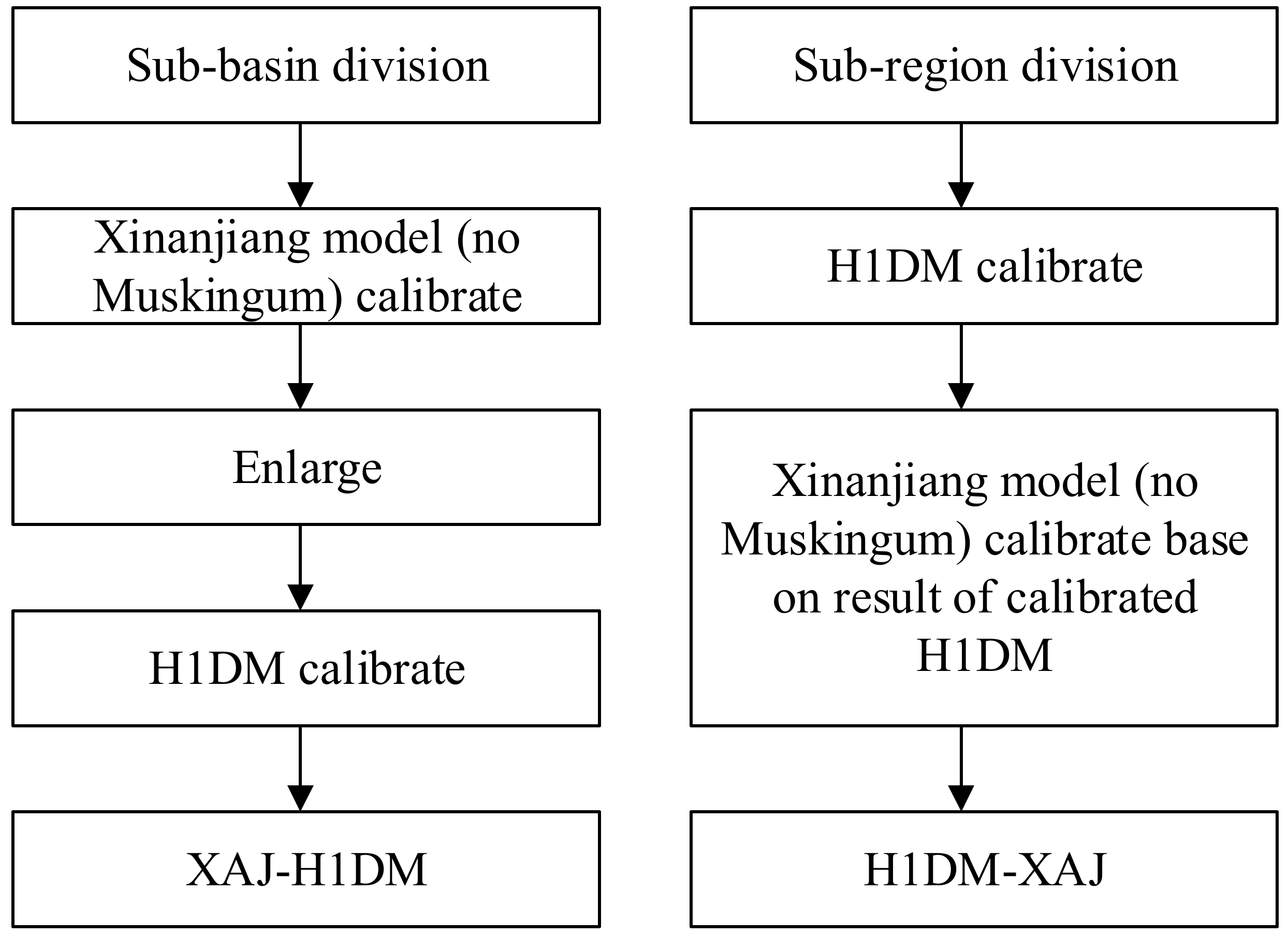
This paper developed the XAJ-H1DM in a loosely coupled way. First, the Xinanjiang model of the sub-catchment in the sub-region are calibrated with observed data and the calibrated parameters were transposed to the catchment in the same sub-region. In the receiving catchment, the hydrology data were gauged. In addition, the one-dimensional hydraulic model was calibrated. Then, the prediction results of the Xinanjiang model are appropriately increased according to the area ratio of the sub-catchment and sub-region. Finally, the increased results are added to the one-dimension hydrodynamic model as the boundary condition of the one-dimensional hydrodynamic model. The flow chart of the XAJ-H1DM and H1DM-XAJ are shown in Figure 3.

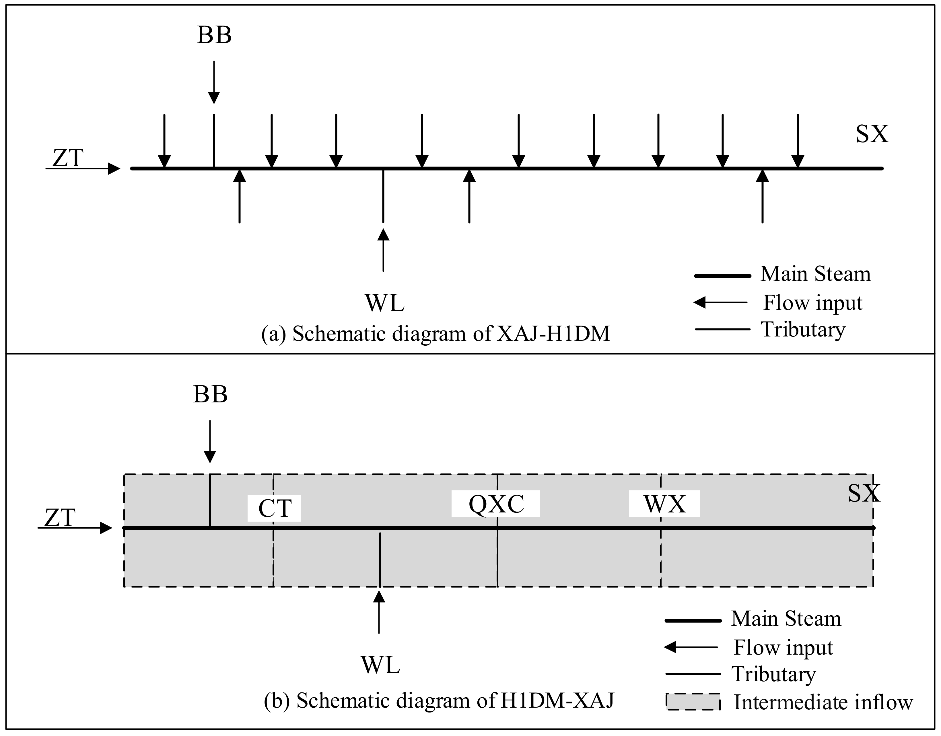
In this coupled model, the upper boundary uses the measured flow from the ZT, BB, and WUL stations, the lower boundary uses the measured water levels in front of the dam during the same period, and the internal boundary uses the results of the Xinanjiang model forecast (Figure 4a).

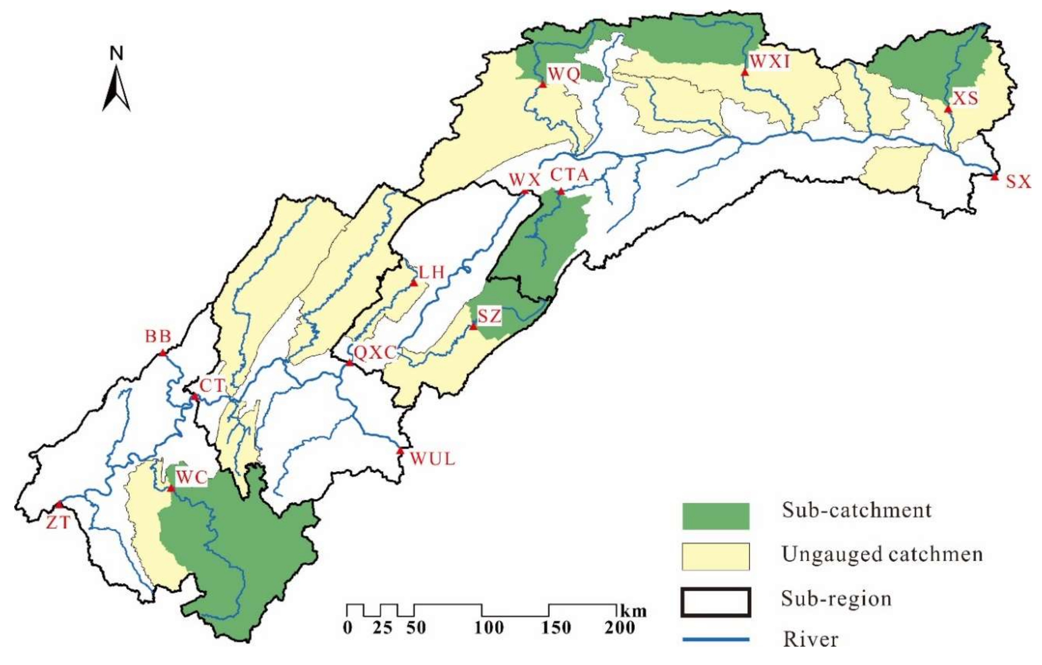
The relative position relationship of sub-catchments and sub-regions is shown in the Figure 5.

2.6.2. H1DM-XAJ Model

In contrast to the previous coupling method, in which the Xinanjiang model and the H1DM model were calibrated independently, in the coupling mode described here, the calibration of the Xinanjiang model was premised on the results of the H1DM model.

First, the H1DM model was separately calibrated, and then the optimization algorithm was used to calibrate the Xinanjiang model, of which the results of the calibrated H1DM model were used as the basis for the coupled model. The results of the one-dimensional hydraulic model used here are fixed and the only the parameters of the Xinanjiang model were calibrated. Finally, the results of the Xinanjiang model are added to the one-dimensional hydrodynamic model as the intermediate flow of the one-dimensional hydrodynamic model. The flow chart of the H1DM-XAJ is shown in Figure 3.

In this coupled model, the Xinanjiang model is used to predict the discharge values of the four sub-regions, which are added to the H1DM model as the intermediate inflow values (Figure 4b).

2.7. Model Calibration and Validation

To compare the performance of the Xinanjiang model to that of the coupled model, four sets of simulations were implemented at a daily time scale: (1) simulations using the Xinanjiang model parameters calibrated at each of the six sub-catchments and four sub-regions; (2) simulations using the H1DM parameters calibrated at the study area; (3) simulations using the XAJ-H1DM model; and (4) simulations using the H1DM-XAJ model.

2.7.1. The Xinanjiang Model

Daily flood events from 2007 to 2008 for each catchment were used for calibration, while the remaining events (daily flood events from 2009) were used for validation. In the period of calibration and validation, the Xinanjiang model was applied to each of the six study catchments and calibrated separately in each individual catchment. All parameters changed within their “reasonable” range based on the literature and/or experience with the model implementation [40].

The shuffled complex evolution (SCE-UA) global optimization algorithm [57] was used to calibrate the model parameters. The objective function for optimizing the parameters is the Nash–Sutcliffe efficiency (NSE) [58] equation, as follows:

$$F_o=1-\frac{1}{N_e}{\displaystyle \sum _{j=1}^{N_e}{E}_{N,j}}$$

(5)

where N_e is the total number of calibration events, and E_N,j is the error indices for the event j.

In accordance with the accuracy standard established by the MWR (Ministry of Water Resources of the People’s Republic of China, 2008) [59], the simulation result is qualified relative to the total runoff volume, peak discharge, and peak time, if the absolute value of the relative runoff volume error (RRE) is less than 20%, if the absolute value of the relative peak discharge error (RPE) is less than 20%, and if the difference in peak time is within a routing period of 3 h, respectively [34]. The values of the objective function range from 0 to 1. A smaller F_o value (close to 0) corresponds to a better match between the simulated streamflow and the observed data. Thus, the parameters were calibrated by minimizing the objective function. Simulations of the sub-regions used a parameter set transposed from their sub-catchments that were expanded according to the area ratio of the sub-region to sub-catchment. The formulas to calculate the RRE, RPE, and peak time error (PTE) values are as follows:

$$RRE=\frac{{\displaystyle \sum _{i=1}^n(R_s-R_o)}}{{\displaystyle \sum _{i=1}^n{R}_o}}\times 100\%$$

(6)

$$RPE=\frac{ma{x}_{i=1}^m(R_s)-ma{x}_{i=1}^m(R_o)}{ma{x}_{i=1}^m(R_o)}\times 100\%$$

(7)

$$PTE=T(ma{x}_{i=1}^m(R_s))-T(ma{x}_{i=1}^m(R_o))$$

(8)

where R_s is the simulation value of flow, R_o is the observation value of flow, n is the total number of years, m is the total number of flood periods in one year, and T(X) represents the day X occurred.

2.7.2. The One-Dimensional Hydrodynamic Model

The simulation time of the hydrodynamic model is set to one year and the time step is set to 900 s. There are three inflow inputs in this model, the ZT hydrometric station flow, BB hydrometric station flow, and WUL hydrometric station flow. In the downstream of the model, the discharge of the model is controlled by the water level of the Fenghuangshan hydrometric station, which is the water level control station of the three gorges reservoir.

The roughness parameter plays a significant role in the hydrodynamic model. Although their values are priori requirements for the solution of the Saint-Venant equations, there have been less definitive measurements of these values. Accurate roughness values are not well established [60]. Roughness is the only parameter that needed to be calibrated in this model.

A trial-and-error method was used to calibrate model parameters. First, the operator selected a set of parameters based on practical experience or existing literature, which was used to drive the model. Then, the simulated value of water level was compared with the measured value in the section that needed to be calibrated. If the measured value was higher than the simulated value, the roughness value was increased; otherwise, the roughness value was decreased. The hydrometric station divides the river into several sections whose roughness values are calibrated in order from downstream to upstream.

The H1DM was calibrated to minimize the mean error of the water level estimation, and the calibrated parameters are listed in

Table 1. Roughness of H1DM.

Subdomains	Range of Roughness
ZT-CT	0.025–0.028
CT-QXC	0.028–0.033
QXC-WX	0.033–0.035
WX-SX	0.035–0.056

. The simulation results obtained were close to those of previous studies [43].

2.8. Parameter Replacement

Hydrologic modeling and parameter replacement were combined to obtain runoff values for this poorly gauged basin. The hydrological similarity among the sub-basins was first analyzed using hierarchical cluster analysis (HCA) [61]. The main factors affecting runoff generation and confluence are the meteorological conditions, basin topography, and underlying surface characteristics [62,63].

In this study, the topographic index was chosen as the defining characteristic of the sub-basins, and in the upstream sub-basins this value was extracted from the DEM. The topographic index, also known as the topographic wetness index (TWI), was developed by Beven and Kirkby [64] within the runoff model TOPMODEL, and is the key factor affecting hydrologic processes. It is defined as $ln\left(\alpha /\beta \right)$, where $\alpha$ is the specific flow accumulation area, specifically, the total flow accumulation area (or upslope area) A through a unit contour length L, and $tan\beta$ is the local slope.

The single flow direction (SFD) algorithm [65], also known as the D8 algorithm, was used to calculate the flow direction. The flow accumulation area (or upslope area) (A) was calculated using a recursive procedure [66]. The specific flow accumulation area (a) was (A) divided by the contour length, which was equal to the grid size or the horizontal resolution of the DEM. The slope was set to be the maximum downward elevation gradient [67].

Therefore, based on the results from HCA, the topographic index probability density distribution curves were also compared for different sub-basins. Finally, parameter replacement was performed for groups with hydrological similarity.

3. Results

The performance of the XAJ-H1DM was investigated to determine whether improved simulations were obtained using the parameters transposed from the donor catchments, and the performances of H1DM-XAJ, XAJ-H1DM, and XAJ models were compared to identify whether improved simulations were obtained from the H1DM-XAJ for ungauged intermediate catchments.

3.1. Results of Xinanjiang Model

The calibrated parameter values of the Xinanjiang module for the three models are listed in

Table 2. List of parameters of the models and the calibrated values for the study catchments.

		Xinanjiang Model				H1DM-XAJ Model				XAJ-H1DM Model
Module	Para	ZT-CT	CT-QXC	QXC-WX	WX-SX	ZT-CT	CT-QXC	QXC-WX	WX-SX	WC	SZ	WQ	CTA	WXI	XS
Evapotranspiration	K	0.500	0.501	1.100	0.953	0.500	0.500	0.500	0.500	0.500	0.500	1.002	0.701	0.587	0.501
	UM	65	75	74	74	65	73	70	71	13	13	26	21	29	16
	LM	76	77	77	61	85	64	65	62	66	66	90	74	79	71
	DM	31	26	37	18	60	15	16	15	15	15	49	15	60	40
	C	0.16	0.11	0.15	0.10	0.14	0.15	0.12	0.13	0.13	0.13	0.11	0.09	0.12	0.16
Runoff generation	IM	0.00	0.03	0.01	0.01	0.03	0.03	0.02	0.01	0.007	0.007	0.030	0.000	0.029	0.023
	B	0.1	0.2	0.2	0.3	0.4	0.2	0.2	0.3	0.1	0.1	0.3	0.4	0.5	0.3
Runoff separation	SM	44.00	16.50	40.81	10.04	22.02	16.72	10.00	10.01	4.55	4.55	1.00	6.93	1.00	8.63
	EX	0.50	0.50	1.16	2.00	0.50	0.50	0.50	0.50	0.66	0.66	0.50	0.50	0.50	0.50
	KI	0.376	0.449	0.350	0.390	0.425	0.380	0.429	0.426	0.450	0.450	0.406	0.450	0.350	0.450
	KG	0.305	0.250	0.350	0.250	0.250	0.250	0.250	0.250	0.252	0.252	0.307	0.350	0.269	0.250
Runoff routing	CS	0.500	0.412	0.164	0.500	0.408	0.500	0.495	0.469	0.410	0.410	0.269	0.273	0.545	0.467
	CI	0.567	0.900	0.754	0.604	0.503	0.565	0.500	0.559	0.691	0.691	0.790	0.900	0.726	0.898
	CG	0.992	0.990	0.998	0.998	0.994	0.990	0.990	0.990	0.998	0.998	0.998	0.996	0.998	0.998
	KE	13.289	2.877	11.324	0.214	-	-	-	-	-	-	-	-	-	-
	XE	0.282	0.000	0.122	0.003	-	-	-	-	-	-	-	-	-	-

K: ratio of potential evapotranspiration to pan evaporation; UM/LM/DM: tension water capacity of upper/lower/deeper layer (mm); C: evapotranspiration coefficient of deeper layer; IM: ratio of impervious area to the total area of the basin; B: exponent of distribution of tension water capacity; SM: free water capacity (mm); EX: exponent of distribution of free water capacity; KI/KG: outflow coefficient of free water storage to interflow/groundwater; CS/CI/CG: recession constant of the lag-and-route method/interflow storage/groundwater storage; KE/XE: Muskingum time constant(h)/weighting factor for each sub-reach. ZT-CT, CT-QXC, QXC-WX and WX-SX stand for the four sub-regions. WC, SZ, WQ, CTA, WXI and XS stand for the six sub-catchments.

. There are 16 parameters in the Xinanjiang model, while the Muskingum parameters (KE and XE) not included in the XAJ-H1DM and H1DM-XAJ models. The outflow is finally routed by the H1DM instead of the Muskingum successive-reaches model in the latter two models to produce the flow at the outlet of the whole catchment. The XAJ-H1DM is applied to sub-catchments, while the remaining models are applied to the sub-regions.

Four evaluation indexes involving the relative runoff volume error (RRE, %), relative peak discharge error (RPE, %), peak time error (PTE, day), and Nash–Sutcliffe efficiency (NSE) are used to evaluate the simulation accuracy of the flow for the four models. The accuracy statistics of flow for the four models are summarized in

Table 3. Accuracy statistics of the four model flow simulations with calibrated parameters for both calibration and validations events.

				2007				2008				2009
		XAJ	H1DM	XAJ-H1DM	H1DM-XAJ	XAJ	H1DM	XAJ-H1DM	H1DM-XAJ	XAJ	H1DM	XAJ-H1DM	H1DM-XAJ
CT	RRE (%)	1.70%	−2.39%	−0.20%	−0.51%	1.76%	−2.54%	−0.83%	−0.67%	2.34%	−3.94%	−2.19%	−1.51%
	RPE (%)	−4.75%	0.78%	1.17%	1.05%	−3.08%	−3.53%	−3.40%	−3.15%	8.77%	−10.95%	−1.92%	−1.32%
	PTE (day)	0	0	0	0	0	0	0	0	0	0	0	0
	NSE	0.9891	0.9960	0.9975	0.9976	0.9909	0.9949	0.9976	0.9976	0.9899	0.9925	0.9975	0.9978
QXC	RRE (%)	3.06%	−5.84%	−3.92%	−1.14%	3.42%	−6.40%	−4.80%	−1.38%	2.82%	−5.56%	−3.68%	−0.57%
	RPE (%)	2.12%	−9.24%	−8.09%	−3.52%	3.12%	−5.18%	−4.39%	−0.88%	1.46%	−15.25%	−5.98%	−1.60%
	PTE (day)	0	0	0	0	0	0	0	0	0	0	0	0
	NSE	0.9910	0.9810	0.9883	0.9955	0.9900	0.9774	0.9827	0.9896	0.9915	0.9776	0.9867	0.9913
WX	RRE (%)	1.01%	−4.68%	−1.84%	2.16%	1.03%	−3.37%	−0.87%	3.92%	1.05%	−3.18%	−0.47%	3.88%
	RPE (%)	−2.90%	−10.77%	−8.42%	−0.72%	0.31%	−2.40%	0.56%	6.94%	−3.77%	−13.69%	−3.87%	2.09%
	PTE (day)	0	0	0	0	0	0	0	0	0	0	0	0
	NSE	0.9930	0.9834	0.9921	0.9951	0.9936	0.9885	0.9936	0.9886	0.9937	0.9864	0.9935	0.9893
SX	RRE (%)	4.80%	−10.19%	−2.28%	3.70%	4.27%	−8.95%	−2.09%	5.63%	3.58%	−7.28%	−0.85%	3.20%
	RPE (%)	6.42%	−20.56%	−14.38%	−2.89%	12.24%	−7.75%	5.27%	6.07%	0.20%	−1.24%	1.76%	8.92%
	PTE (day)	0	0	0	0	−1	0	0	0	0	0	0	0
	NSE	0.9776	0.9212	0.9766	0.9915	0.9808	0.9426	0.9871	0.9788	0.9895	0.9524	0.9803	0.9750

RRE, RPE, PTE and NSE stand for relative runoff volume error, relative peak discharge error, peak time error and Nash–Sutcliffe efficiency.

, which shows the absolute means with respect to the RRE, RPE, PTE, and NSE values for the calibration and validation periods.

For the Xinanjiang model, the absolute means of the RRE, RPE, and PTE values in the simulations for the four study regions range from 1.01% to 4.8%, −4.75% to 12.24% and 0 to −1 day, respectively (Table 2). The PTE values of the Xinanjiang model simulations are mostly zero at a daily time scale except in one special case (Table 2 result of SX in 2008). The NSE values vary between 0.9776 and 0.9937. These results indicate that the Xinanjiang model is capable of reproducing both the magnitude and dynamics of the observed flood events at different catchment scales once its parameters are calibrated.

3.2. Results of the H1DM Model

For the H1DM model, the absolute means of the RRE and RPE simulations for the four study regions range from −10.19% to −2.3% and −20.56% to 0.78%, while the PTE is always 0 days (Table 2). The NSE varies between 0.9212 and 0.9960 (Table 2), indicating that the H1DM model can reasonably simulate the general shapes of the storm hydrographs when calibrated singly. This suggests that the H1DM model is highly capable of simulating the total runoff volume and has an inferior capability to simulate the peak discharge when only the two main tributaries were taken into consideration in these catchments. However, the original Xinanjiang model shows relatively better performance in simulating the total runoff volume and the peak values of discharge in all catchments and periods, since both the main tributaries and rainfall-runoff values in the catchments are reasonably simulated in the original Xinanjiang model.

Three additional evaluation indexes, the absolute mean water level error (AMWE, m), relative maximum water level error (RMWE, %), and Nash–Sutcliffe efficiency (NSE), are used to evaluate the simulation accuracy of water level for the four models, as follows:

$$AMWE=\frac{1}{n}{\displaystyle \sum _{i=1}^n({\eta }_s-{\eta }_o)}$$

(9)

$$RMWE=\frac{ma{x}_{i=1}^m({\eta }_s)-ma{x}_{i=1}^m({\eta }_o)}{ma{x}_{i=1}^m({\eta }_o)}$$

(10)

where ${\eta }_s$ is the simulation water level, ${\eta }_o$ is the observation water level, n is the total number of years, and m is the total number of flood periods in one year.

The accuracy statistics of the water level for the three models’ performances are summarized in

Table 4. Accuracy statistics of the four model water level simulations with calibrated parameters for both calibration and validations events.

				2007				2008				2009
		XAJ	H1DM	XAJ-H1DM	H1DM-XAJ	XAJ	H1DM	XAJ-H1DM	H1DM-XAJ	XAJ	H1DM	XAJ-H1DM	H1DM-XAJ
CT	AWME (m)	-	−0.340	−0.204	−0.237	-	−0.215	−0.112	−0.099	-	−0.114	−0.028	0.003
	RMWE (%)	-	−0.76%	−0.74%	−0.74%	-	−0.64%	−0.60%	−0.60%	-	−2.19%	−1.37%	−1.38%
	NSE	-	0.9839	0.9885	0.9867	-	0.9922	0.9942	0.9943	-	0.9890	0.9938	0.9940
QXC	AWME (m)	-	−0.046	0.046	0.132	-	0.017	0.083	0.180	-	−0.044	0.015	0.083
	RMWE (%)	-	−1.09%	−0.88%	−0.36%	-	−0.13%	0.03%	0.05%	-	−0.04%	−0.03%	−0.02%
	NSE	-	0.9896	0.9934	0.9920	-	0.9993	0.9990	0.9977	-	0.9991	0.9995	0.9990
WX	AWME (m)	-	−0.046	0.026	0.064	-	0.007	0.057	0.096	-	−0.009	0.030	0.061
	RMWE (%)	-	−0.02%	−0.01%	0.02%	-	−0.01%	0.06%	0.07%	-	−0.01%	0.00%	0.01%
	NSE	-	0.9966	0.9981	0.9974	-	0.9998	0.9996	0.9993	-	0.9998	0.9987	0.9995
SX	AWME (m)	-	0.000	0.000	0.000	-	0.000	0.000	0.000	-	0.000	0.000	0.000
	RMWE (%)	-	0.00%	0.00%	0.00%	-	0.00%	0.00%	0.00%	-	0.00%	0.00%	0.00%
	NSE	-	1.0000	1.0000	1.0000	-	1.0000	1.0000	1.0000	-	1.0000	1.0000	1.0000

AWME, RMWE and NSE stand for absolute mean water level error, relative maximum water level error and Nash–Sutcliffe efficiency.

, which shows the absolute means with respect to the AMWE, RMWE, and NSE values for the calibration and validation periods. Meanwhile, the AMWE and RMWE simulations for the four study regions range from 0 m to −0.34 m and 0% to −2.19%, respectively. The NSE values of the water level vary between 0.9839 and 1 (Table 4). The water level simulations and observations are almost identical in SX because the water level was set as the downstream boundary of the H1DM model while SX was too close to the downstream boundary to avoid the influence.

Relative to the flow simulations of H1DM model, the water level simulations show a superior performance in NSE since the roughness, the only parameter calibrated in the H1DM model, only affects the water level simulations. In other words, the water level simulations can be adjusted to the best state but the flow simulations cannot be adjusted once the boundary conditions of H1DM are confirmed. The roughness values are listed in Table 1. Table 3 shows that the validated roughness values are basically consistent with those of previous studies. These results indicate that the H1DM model is capable of reproducing both the flow and water levels of observed flood events once its parameters are calibrated.

3.3. Results for Parameter Replacement

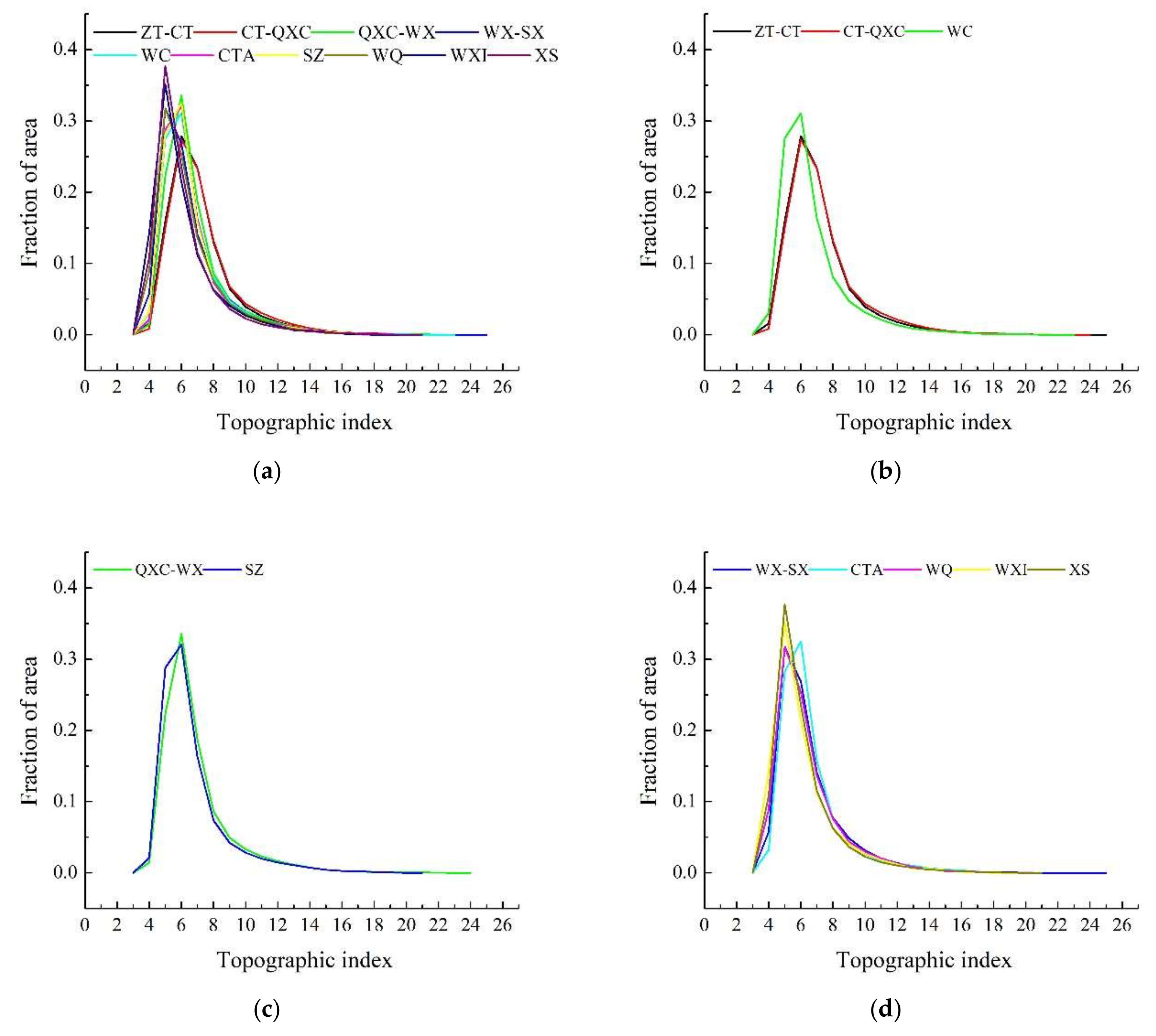
The physical characteristics among the 6 sub-basins and the 4 sub-regions upstream of the Three Gorges Reservoir Basin showed distinct differences. The topographic index probability density distribution curves were compared among the 10 regions (Figure 6a). Based on the topographic index probability density distribution and the locations, the 10 regions were divided into three categories.

Finally, three groups with hydrological similarities were obtained from the results of the topographic index probability density distribution curve, and parameter replacement could then be conducted within each group.

For the XAJ-H1DM model, the ungauged catchments were modeled using the calibrated parameter sets from similar catchments in the same sub-region.

The donor catchments for the receptor catchments listed in

Table 5. Accuracy statistics of the Xinanjiang module in XAJ-H1DM.

Catchment	NSE
	2007	2008	2009	Average
WC	0.514	0.799	0.826	0.713
SZ	0.291	0.223	0.235	0.249
WQ	0.848	0.662	0.832	0.781
CTA	0.741	0.741	0.590	0.690
WXI	0.830	0.330	0.394	0.518
XS	0.640	0.642	0.602	0.628

were selected according to their locations (see Figure 4) and topographic index probability density distribution. For ZT-CT sub-region and CT-QXC sub-region, model parameters were transposed from a single donor catchment, i.e., WC. For QXC-WX sub-region, model parameters were transposed from SZ catchment, while multiple donor catchments were used for WX-SX sub-region. The inflows of the hydrodynamic model in the coupled model increased from 3 to 15, while the output controlled by the water level remained the same.

3.4. Results of XAJ-H1DM Model

The calibrated parameter values of the Xinanjiang module of XAJ-H1DM for each sub-catchment are listed in Table 2. The accuracy statistics of the model performance are summarized in Table 5, which represents the annual NSE values and the average NSE values for the separate calibration and validation flood events. For all sub-catchments, since all watersheds are mesoscale, and from small watersheds and the Xinanjiang module was only used to simulate runoff, the Muskingum module in runoff routing was not included in the Xinanjiang module.

According to Table 5, the NSE values for SZ were 0.291, 0.223 and 0.235 from 2007 to 2009. There are two possible explanations for this result: the catchment area is too small, and the outflow of the catchment during this period is too small (less 350 m³/s). The NSE values for WX were 0.33 and 0.394 from 2008 to 2009. The terrain in the WX sub-catchment is complex, ravines and gullies crisscross the area, the flood routing time is short; therefore, the simulation results of the Xinanjiang module without the routing module will produce large errors. This may indicate that the major source of uncertainty in the application of the Xinanjiang module in these ungauged catchments lies in the model process of runoff routing [27].

In addition to the above conditions, the Xinanjiang module performs well, and NSE is higher than 0.5 for all remaining flood events. For all calibration and validation events, the average NSE values for the six study sub-catchments range from 0.249 to 0.781. In general, the simulations of the Xinanjiang module can be used to simulate rainfall-runoff accurately. According to the relative position and the nesting relationship of the basin, the parameters of the Xinanjiang module in sub-catchments are simply transposed to the sub-regions.

Table 3 and Table 4 provide the accuracy statistics of the XAJ-H1DM model results by coupling the singly calibrated Xinanjiang model with the singly calibrated H1DM model. The simulations by the XAJ-H1DM model show obvious improvement for the RRE and RPE metrics relative to those of the single H1DM model. The RRE and RPE tremendously improved at SX in 2007, form −10.19% to −2.28% and from −20.56% to 14.38% (Table 2). It is not surprising that the performance of XAJ-H1DM model has a remarkable improvement than H1DM model in all aspects. For the results of water level (Table 4), relative to H1DM model, both the simulations of AWME and the simulations of RMWE have decreased for XAJ-H1DM in varying degrees, while their NSE increased accordingly.

Collective analysis of the simulation results shown in Table 3 and Table 4 clarifies that the XAJ-H1DM model outperforms the H1DM model in most cases and can be compared with Xinanjiang model. Moreover, extra simulations, such as water level and water surface profile in any reach, can be obtained from the XAJ-H1DM model. Therefore, it is evident that the integrated hydrologic and hydrodynamic model has the ability to simulate floods using the regionalization approaches.

3.5. Results of H1DM-XAJ Model

To address the issue of the simulation results of the XAJ-H1DM model not being satisfactory with regard to ungauged intermediate catchments, another coupled model (H1DM-XAJ model) is proposed. For the H1DM-XAJ model, four Xinanjiang models established to predict intermediate flow were applied to ZT-CT, CT-QXC, QXC-WX, and WX-SX sub-regions. The calibration of H1DM module in H1DM-XAJ model and the calibration of a single H1DM model are the same. The calibration of Xinanjiang module in H1DM-XAJ model is different from the calibration of Xinanjiang module in XAJ-H1DM model and the single Xinanjiang model. In other words, there are four different Xinanjiang parameter sets for all four models. The calibration method and the calibration target are the same as the previous model.

In this coupling mode, the calibration of the Xinanjiang model is based on the results of the H1DM model. The calibrated parameter values of the Xinanjiang module of H1DM for each sub-catchment are listed in Table 2. The accuracy statistics of the H1DM-XAJ model performance are summarized in Table 3 and Table 4. The absolute means of RRE and RPE simulations for the four study regions range from −1.51% to 5.63% and −3.52% to 6.97%, while the PTE is always 0 day (Table 3). The NSE varies between 0.9760 and 0.9976. From Table 4, it is evident that the AMWE and RMWE simulations for the four study regions range from 0 m to 0.237 m and 0% to 1.38%, respectively. These indicate that the H1DM-XAJ model shows a veracious simulation and can be compared with other models.

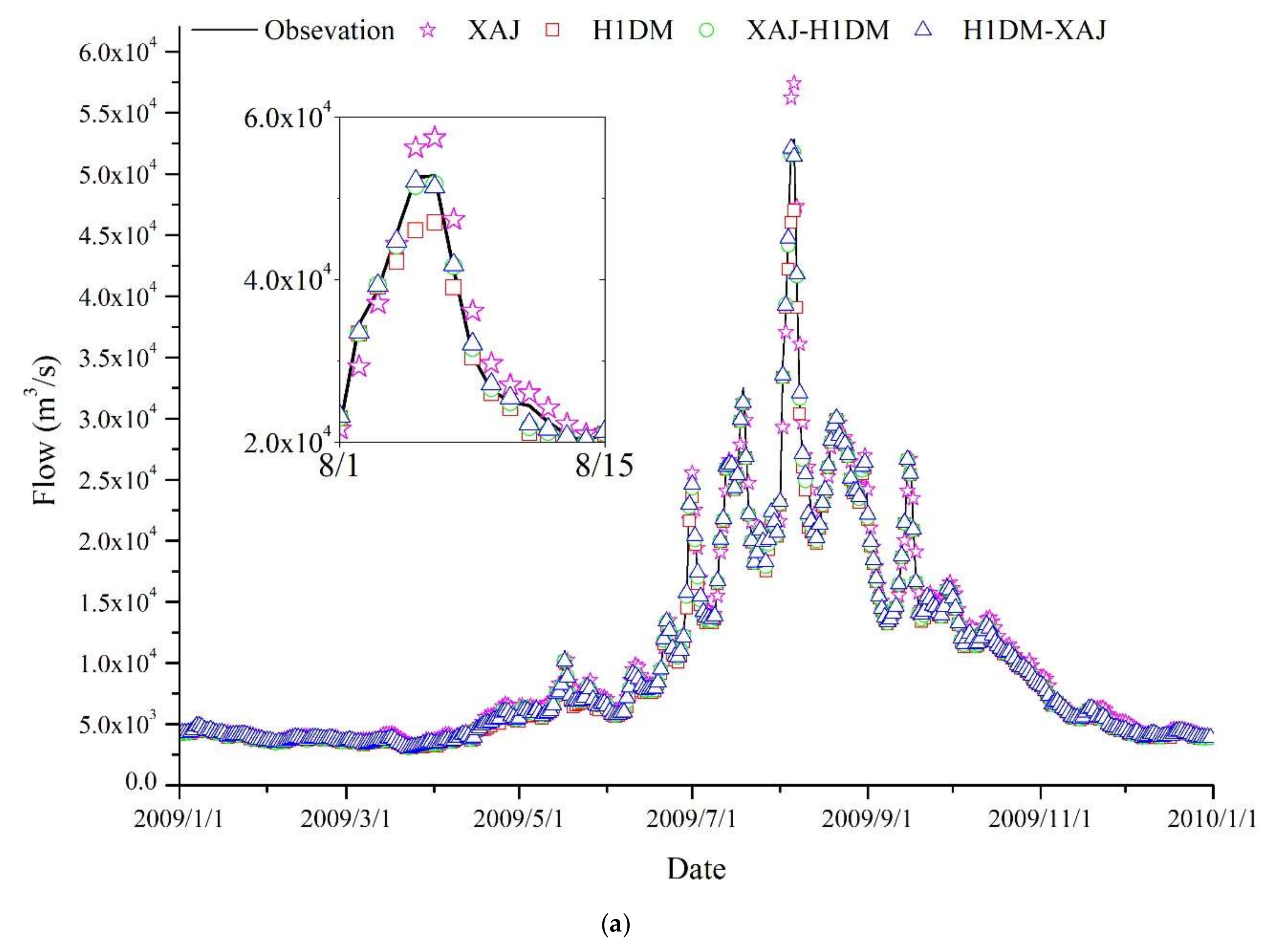
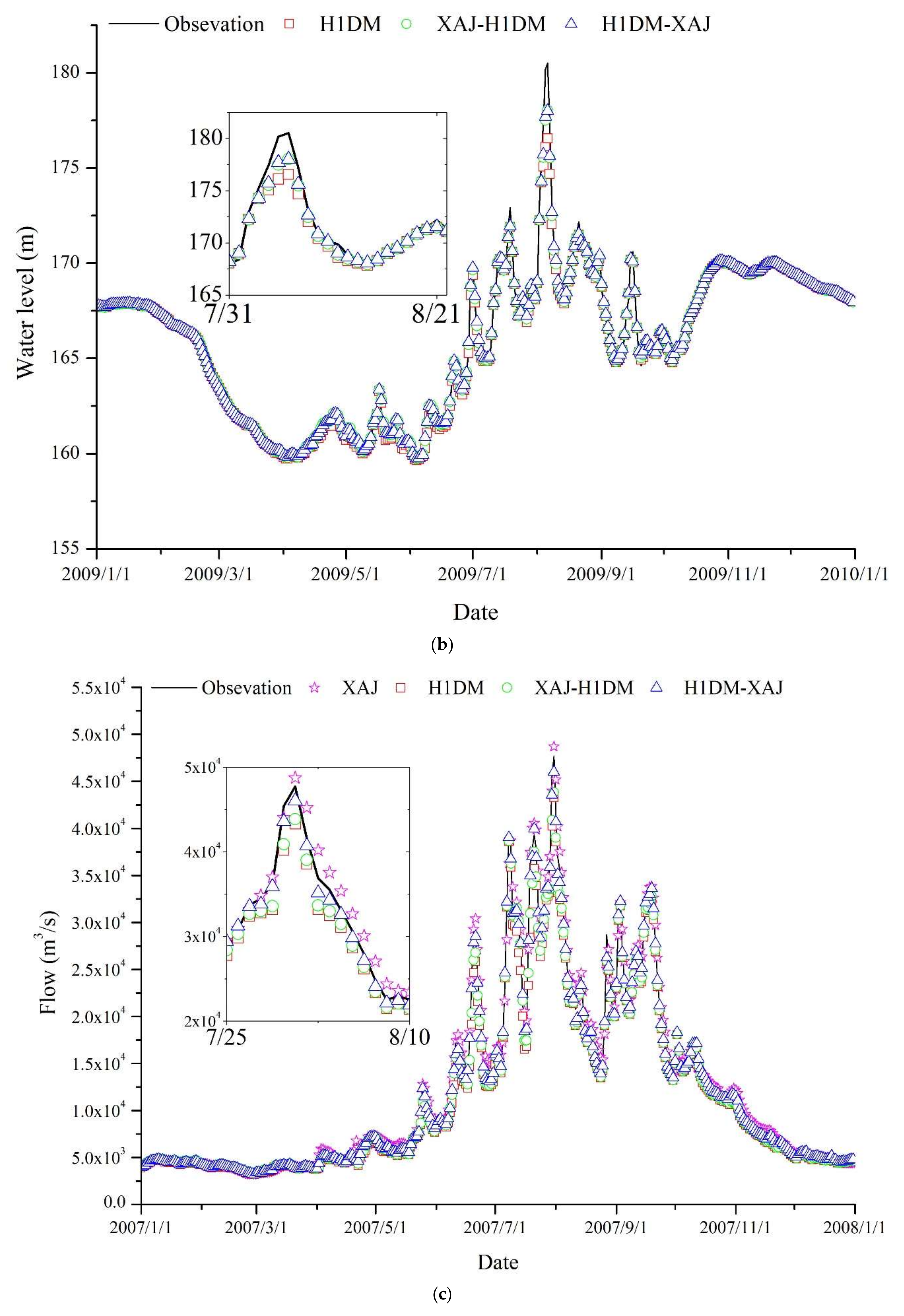
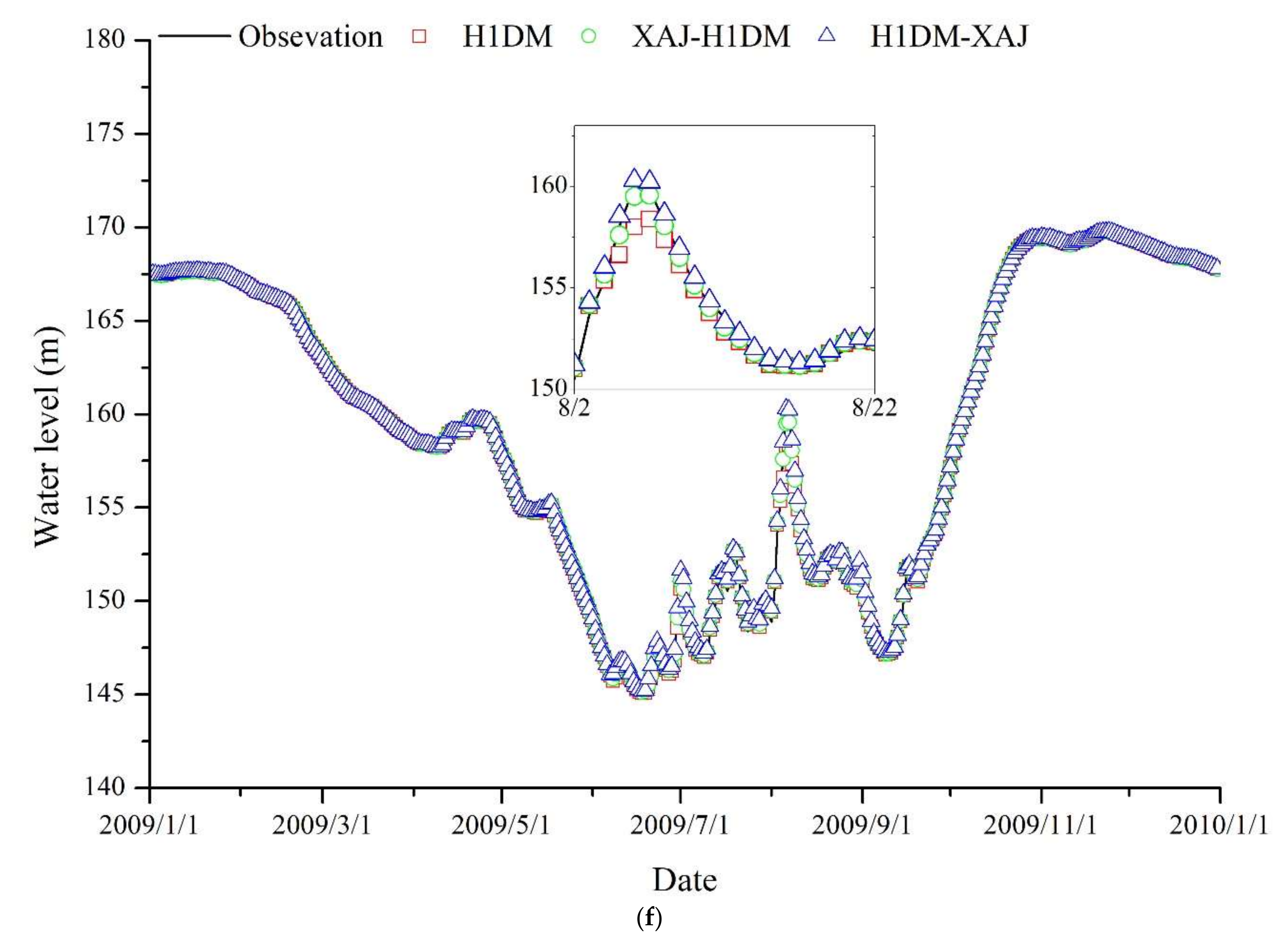
In addition, the water level and discharge curves of several stations are shown in Figure 7 that allow the comparison of the results of the coupled model. As can be seen from the figure, H1DM-XAJ performs well in most cases, and the simulation accuracy of water level and flow is higher than that for other models. Especially regarding the peak simulation, the H1DM-XAJ model is better than other models.

4. Discussion

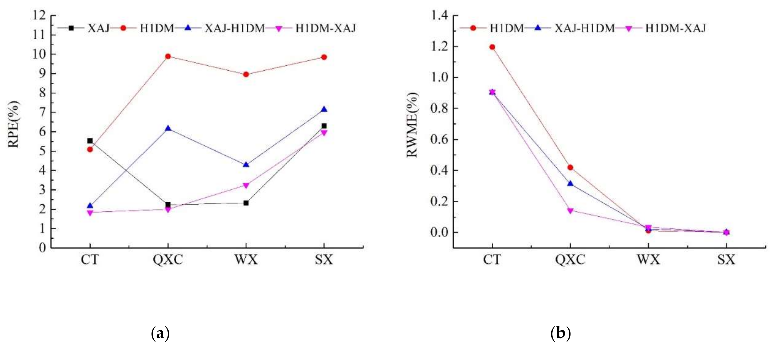
To compare the simulation results of the four models more intuitively, the contents of Table 3 and Table 4 are rearranged and are shown as Figure 8, Figure 9 and Figure 10. The absolute values of all metrics were taken and were averaged with respect to time. These were then plotted according to the sequence of the hydrological stations. As can be seen from Figure 8, RRE of H1DM-XAJ model is significantly smaller than that of other models in CT and QXC, while XAJ-H1DM model replaces the position of H1DM-XAJ in WX and SX. The difference between H1DM-XAJ and XAJ-H1DM is the simulations of rainfall-runoff in Xinanjiang module. Therefore, the simulations of rainfall-runoff were overrated by H1DM-XAJ model in WX and SX.

According to Figure 8, the performance of RPE in these four models shows a similar outcome. Meanwhile, the simulations in terms of NSE are larger than 0.98 for all sub-regions except for the single H1DM model (Figure 9). According to Figure 8b, H1DM-XAJ and XAJ-H1DM show worse results in AMWE. The reason for this may be that the simulations of H1DM model have been calibrated to the best status before the simulations of the Xinanjiang model were taken into account. Therefore, the addition of simulations of the Xinanjiang model made the average water level too high. On the contrary, with the addition of the Xinanjiang model, the ability of the coupled models to simulate the flood peak improved (Figure 8b), and the fitting degree of water level process line also increased (see Figure 9b). These show that the Xinanjiang model, the XAJ-H1DM model, and the H1DM-XAJ model, once calibrated with parameters, were able to reproduce the magnitude and dynamics of observed flood events on different catchment scales. Furthermore, the H1DM-XAJ model performed better than the other three in majority of the instances and showed obvious improvement compared with the other two.

Table 6. Ratio of intermediate flow to the gaged inflow.

Catchment	2007	2008	2009
ZT-CT	2.22%/1.5%	1.83%/2.09%	1.88%/2.55%
CT-QXC	2.08%/3.94%	1.97%/5.26%	2.12%/5.38%
QXC-WX	3.15%/5.94%	2.85%/7.45%	2.92%/7.38%
WX-SX	8.06%/12.02%	7.07%/14.47%	6.64%/13.85%

Note: Label “/” is used to separate two data of the two models, XAJ-H1DM and H1DM-XAJ.

presents the ratio of the intermediate inflow calculated by the two coupled models to the measured flow at the downstream site. The intermediate inflow is relatively small, and the intermediate inflow has little effect on the simulation results, which explains why the NSE values of the two models do not change much. In addition, from upstream to downstream of the river basin, the proportion of intermediate inflow gradually increased, which may be related to the steep terrain of the downstream river basin and the amount of rainwater.

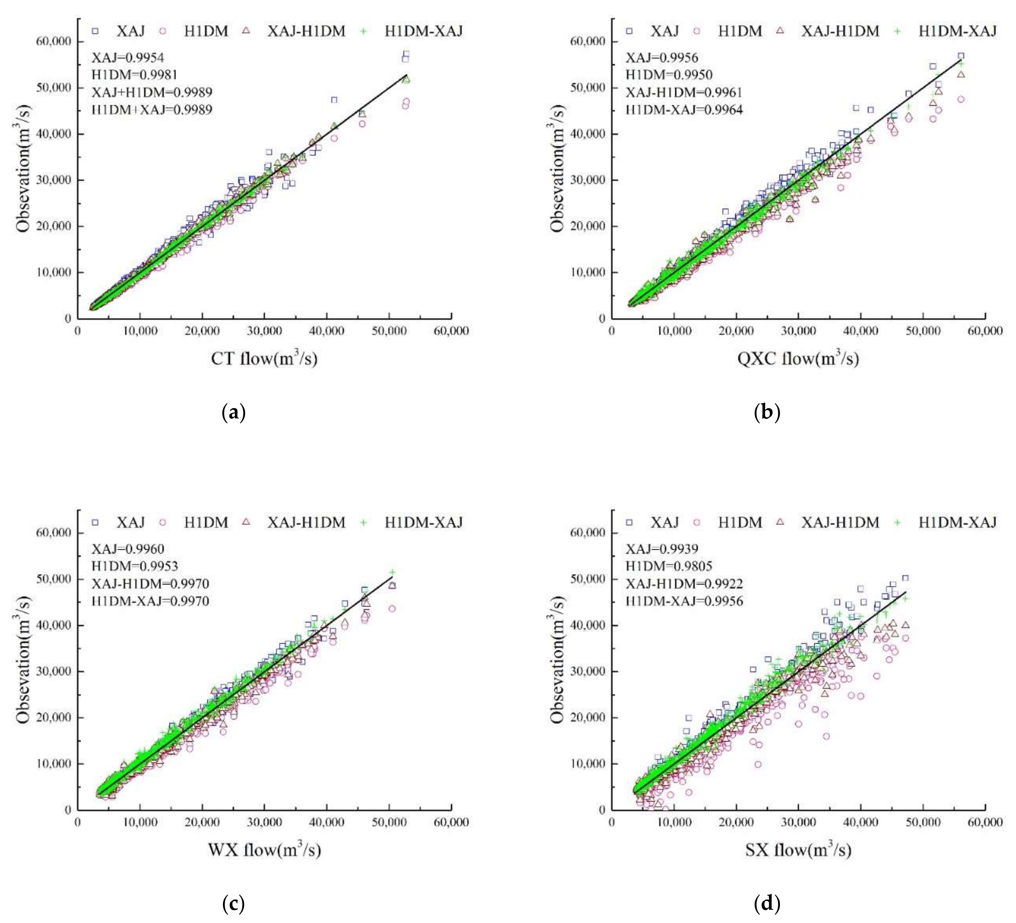
The above discussion is based on the results obtained from a simple comparison of the evaluation indexes. We further discuss the model performance by comparing the flood simulation capabilities of the four models for different catchments. In this approach, the correlation coefficient R² [68] is used as a similarity index on the basis of the analysis of Figure 11. Furthermore, Figure 11 illustrates the R² between the flow simulations of the four models and the measured values at different hydrometric stations, while the R² of water level simulations are presented in Figure 12.

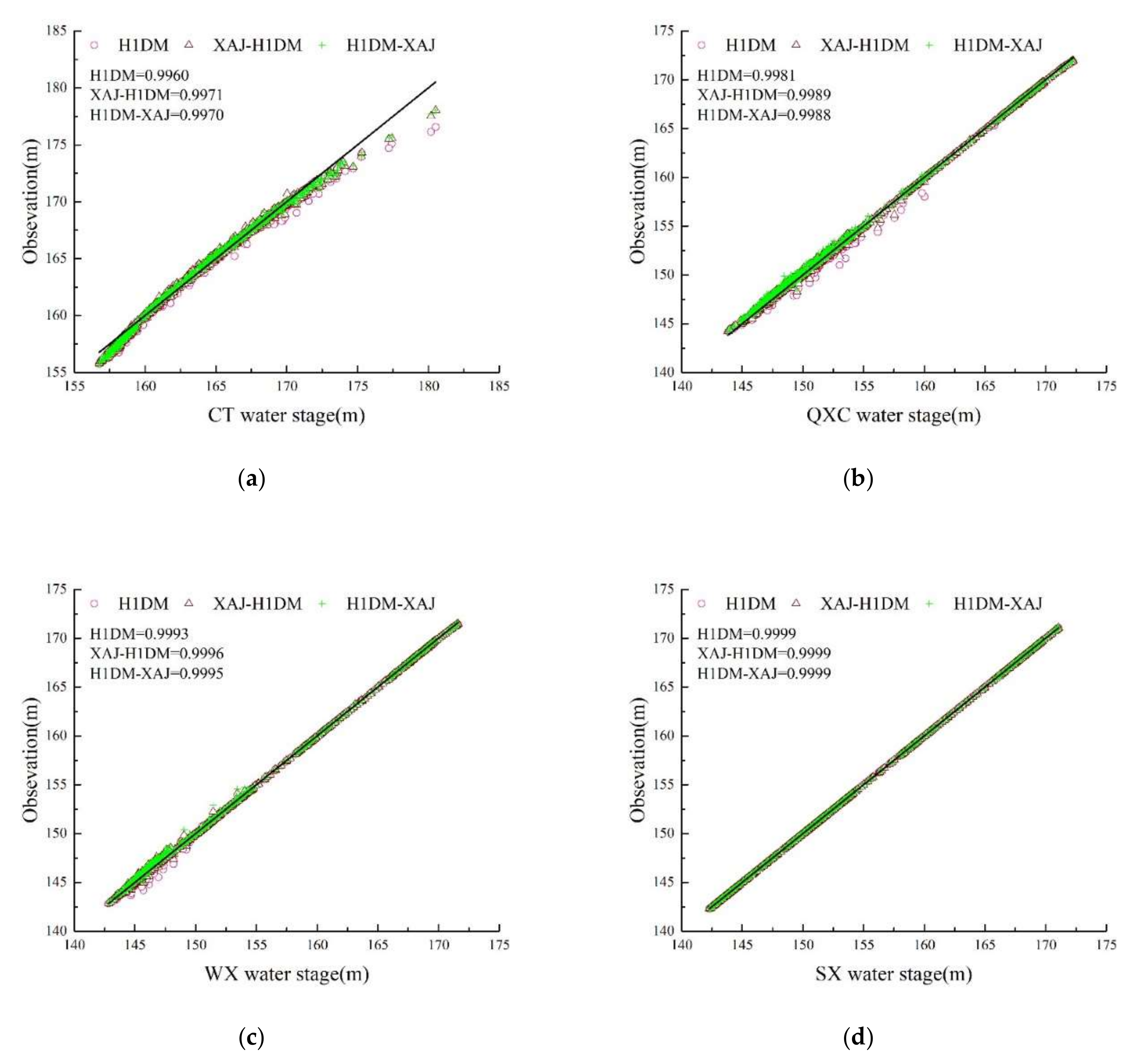
The simulation results of the four models are distributed around the measured values, and the simulation results of the coupled models are more densely distributed than the single Xinanjiang model and the H1DM model. In addition, relative to XAJ-H1DM model, simulation results of H1DM-XAJ model are more uniformly and intensively distributed (see Figure 11 and Figure 12). It is worth mentioning that the H1DM model shows several extreme anomalies in SX, which may be due to the fact that SX is too close to the Three Gorges Dam, and H1DM does not consider the huge inflows of tributaries contributing to the mainstream flow.

In addition, the simulations of the H1DM-XAJ model are much better than those of the other three models. The Xinanjiang model tends to overestimate the flow value, while the XAJ-H1DM model does the opposite; the latter always simulates a smaller simulation value than the real data. H1DM has a more balanced simulation capability, and simulation results are always evenly distributed around the observed values. These conclusions justify the results presented in Table 3 and Table 4. In terms of water level simulation results, compared with the single H1DM model, the coupled models also showed a significant improvement (see Figure 11 and Figure 12).

The coupled models perform better when simulating middle water levels relative to simulated high and low water levels, and the simulation results are closer to the real measurements when simulating middle water levels (Figure 12a). In addition, hydrodynamic models tend to simulate smaller results than the actual values at the CT station. The possible reason for this phenomenon is that CT is located near the end of the backwater fluctuation area of the Three Gorges Reservoir; the riverbed is silted, which results in the deviation between the topographic data and the measured data. Based on the results presented here and the aforementioned similarity analysis of flow and water level, it is suggested that the coupled model, developed by coupling Xinanjiang model with H1DM model, is more likely suitable for simulation of flood in the Three Gorges Reservoir, and has the potential to produce substantially improved flood simulations in this ungauged intermediate catchment.

The calculations of the XAJ-H1DM and H1DM-XAJ models are almost the same. However, the structures of the two models are different, with H1DM-XAJ being better than XAJ-H1DM in terms of model structure and simulation results. In addition, the calculation volume of the two integrated models is larger than that of the single Xinanjiang model, requiring more data and outputting more results. Coupling the hydrological model with the hydrodynamic model can overcome the shortcomings of the single hydrological model that cannot predict the water level and the lack of accuracy of the single hydrodynamic model due to the lack of intermediate inflow simulation. Moreover, it combines the advantages of both models and takes rainfall as well as terrain information into consideration.

The models proposed in this paper integrate hydrological and hydrodynamic models in the simplest coupling way. Compared with other fully integrated distributed models, such as the coupled model of MIKE11 and MIKE SHE [19], the model proposed in this paper has some limitations:

• in the simulation of rainfall-runoff, only the effects of rainfall and evaporation on the runoff generation and routing in the basin were considered, and no consideration was given to meteorological factors (such as humidity, wind direction), land use, and vegetation cover;
• compared with the distributed hydrological model, the Xinanjiang model is faster in the calculation and requires less data, but the physical meaning is not clear enough and there are more empirical parameters;
• the H1DM used in this paper has fast calculation speed and high accuracy but does not consider the different roughness of the riverbed and the flood plain.

However, the coupling way proposed in this paper has proven to be effective, and the integrated model also has reliable accuracy that can be applied to flood simulation.

5. Conclusions

One-dimensional hydrodynamic models are very useful in simulating flood routing in natural rivers, but most studies often do not take intermediate inflows into account because of the difficulty in obtaining the data regarding intermediate flows. In view of the deficiencies of the general one-dimension hydrodynamic model, we proposed its coupling with the Xinanjiang model and produce two coupled models, namely the XAJ-H1DM and H1DM-XAJ models, which differed in their manner of coupling.

For the XAJ-H1DM model, the Xinanjiang model and the H1DM model were separately calibrated, and the results of the Xinanjiang model in the coupled model were derived from the Xinanjiang model for the enlarged sub-catchment; the results were verified by a small amount of gauged data. In the H1DM-XAJ model, H1DM model was calibrated first, and then the Xinanjiang model was calibrated on the basis of the already calibrated H1DM model for each catchment. The four models were applied to a poorly gauged catchment, Three Gorges Reservoir Region, where the intermediate runoff cannot be obtained directly but can be predicted by the rainfall-runoff model.

In this study, we evaluated the flood simulation capability of the Xinanjiang model, H1DM model and two coupled models at the daily time scale for the purpose of improving the capability of flood simulation in ungauged intermediate catchments.

• Results indicate that the regionalization approaches can be successfully used in the application of the integrated hydrologic and hydrodynamic model.
• Our results show that both coupled models are capable of providing satisfactory and comparative simulations of runoff volume, peak discharge, peak time, and flood hydrograph for the data-scarce catchments once they are well-calibrated. Integrated models also have the ability to simulate floods using the regionalization approaches. The coupled models produced markedly improved estimates of peak discharge and runoff volume as compared to the single H1DM model, indicating that the intermediate flow is a major uncertainty source for the application of the H1DM model in large scale watersheds. Coupling Xinanjiang with H1DM has the potential to substantially improve the flood simulation capability of the H1DM model in poorly gauged catchments.
• The coupled models have shown improvements in peak discharge, runoff volume, peak time, and hydrograph as compared to the XAJ model. Moreover, the ability of the coupled models to simulate peak water level and hydrograph, which any hydrological model lack, is significantly better than that of the single H1DM model. This study demonstrates the importance of incorporating intermediate inflows, which can be obtained from rainfall-flow model predictions in data-deficient areas, in hydraulic models.
• The coupled way of the H1DM-XAJ model provides a realizable direction to improve the flood simulation capability of the integrated hydrologic and hydrodynamic models in ungauged intermediate catchments.

The presented framework can be applied to other data-scarce catchments worldwide to gain a better understanding of the hydrodynamic processes.

References

- Todini, E. Rainfall-Runoff Models for Real-Time Forecasting. Encycl. Hydrol. Sci. 2006. [Google Scholar] [CrossRef]
- WMO. Manual on Flood Forecasting and Warning; World Meteorological Organization: Geneva, Switzerland, 2011. [Google Scholar]
- Alho, P.; Aaltonen, J. Comparing a 1D hydraulic model with a 2D hydraulic model for the simulation of extreme glacial outburst floods. Hydrol. Process. Int. J. 2008, 22, 1537–1547. [Google Scholar] [CrossRef]
- Anderson, E.J.; Schwab, D.J.; Lang, G.A. Real-time hydraulic and hydrodynamic model of the St. Clair River, Lake St. Clair, Detroit River system. J. Hydraul. Eng. 2010, 136, 507–518. [Google Scholar] [CrossRef] [Green Version]
- Brunner, G.W. HEC-RAS River Analysis System. Hydraulic Reference Manual. Version 1.0; Hydrologic Engineering Center: Davis, CA, USA, 1995. [Google Scholar]
- Correia, F.N.; Rego, F.C.; Saraiva, M.D.G.; Ramos, I. Coupling GIS with hydrologic and hydraulic flood modelling. Water Resour. Manag. 1998, 12, 229–249. [Google Scholar] [CrossRef]
- Liu, Q.; Qin, Y.; Zhang, Y.; Li, Z. A coupled 1D–2D hydrodynamic model for flood simulation in flood detention basin. Natl. Hazards 2015, 75, 1303–1325. [Google Scholar] [CrossRef]
- Mu, J.-B.; Zhang, X.-F. Real-time flood forecasting method with 1-D unsteady flow model. J. Hydrodyn. 2007, 19, 150–154. [Google Scholar] [CrossRef]
- Nandalal, K. Use of a hydrodynamic model to forecast floods of Kalu River in Sri Lanka. J. Flood Risk Manag. 2009, 2, 151–158. [Google Scholar] [CrossRef]
- Panda, R.K.; Pramanik, N.; Bala, B. Simulation of river stage using artificial neural network and MIKE 11 hydrodynamic model. Comput. Geosci. 2010, 36, 735–745. [Google Scholar] [CrossRef]
- Seyoum, S.D.; Vojinovic, Z.; Price, R.K.; Weesakul, S. Coupled 1D and noninertia 2D flood inundation model for simulation of urban flooding. J. Hydraul. Eng. 2011, 138, 23–34. [Google Scholar] [CrossRef]
- Shamsudin, S.; Hashim, N. Rainfall runoff simulation using MIKE11 NAM. Malays. J. Civ. Eng. 2002, 15, 26–38. [Google Scholar]
- Ye, J.; McCorquodale, J. Simulation of curved open channel flows by 3D hydrodynamic model. J. Hydraul. Eng. 1998, 124, 687–698. [Google Scholar] [CrossRef]
- Jiang, J. Coupled Modeling and Application of Hydrological, Hydrodynamic and Water Quality Models for Typical Coastal Basins: A Case Study of the Yongjiang River Basin. Ph.D. Thesis, Zhejiang University, Hangzhou, China, 2018. [Google Scholar]
- Xu, Z.; Godrej, A.N.; Grizzard, T.J. The hydrological calibration and validation of a complexly-linked watershed—Reservoir model for the Occoquan watershed, Virginia. J. Hydrol. 2007, 345, 167–183. [Google Scholar] [CrossRef]
- Inoue, M.; Park, D.; Justic, D.; Wiseman Jr, W.J. A high-resolution integrated hydrology—Hydrodynamic model of the Barataria Basin system. Environ. Model. Softw. 2008, 23, 1122–1132. [Google Scholar] [CrossRef]
- Morita, M.; Yen, B.C. Modeling of conjunctive two-dimensional surface-three-dimensional subsurface flows. J. Hydraul. Eng. 2002, 128, 184–200. [Google Scholar] [CrossRef]
- Lian, Y.; Chan, I.-C.; Singh, J.; Demissie, M.; Knapp, V.; Xie, H. Coupling of hydrologic and hydraulic models for the Illinois River Basin. J. Hydrol. 2007, 344, 210–222. [Google Scholar] [CrossRef]
- Liu, H.-L.; Chen, X.; Bao, A.-M.; Wang, L. Investigation of groundwater response to overland flow and topography using a coupled MIKE SHE/MIKE 11 modeling system for an arid watershed. J. Hydrol. 2007, 347, 448–459. [Google Scholar] [CrossRef]
- De Paiva, R.C.D.; Buarque, D.C.; Collischonn, W.; Bonnet, M.P.; Frappart, F.; Calmant, S.; Bulhoes Mendes, C.A. Large-scale hydrologic and hydrodynamic modeling of the Amazon River basin. Water Resour. Res. 2013, 49, 1226–1243. [Google Scholar] [CrossRef] [Green Version]
- Paiva, R.; Collischonn, W.; Bonnet, M.-P.; De Goncalves, L.; Calmant, S.; Getirana, A.; Santos da Silva, J. Assimilating in situ and radar altimetry data into a large-scale hydrologic-hydrodynamic model for streamflow forecast in the Amazon. Hydrol. Earth Syst. Sci. 2013, 17, 2929–2946. [Google Scholar] [CrossRef] [Green Version]
- Mateo, C.M.; Hanasaki, N.; Komori, D.; Tanaka, K.; Kiguchi, M.; Champathong, A.; Sukhapunnaphan, T.; Yamazaki, D.; Oki, T. Assessing the impacts of reservoir operation to floodplain inundation by combining hydrological, reservoir management, and hydrodynamic models. Water Resour. Res. 2014, 50, 7245–7266. [Google Scholar] [CrossRef]
- Bellos, V.; Tsakiris, G. A hybrid method for flood simulation in small catchments combining hydrodynamic and hydrological techniques. J. Hydrol. 2016, 540, 331–339. [Google Scholar] [CrossRef]
- Zhang, L.; Lu, J.; Chen, X.; Liang, D.; Fu, X.; Sauvage, S.; Sanchez Perez, J.-M. Stream flow simulation and verification in ungauged zones by coupling hydrological and hydrodynamic models: A case study of the Poyang Lake ungauged zone. Hydrol. Earth Syst. Sci. 2017, 21, 5847–5861. [Google Scholar] [CrossRef] [Green Version]
- Wu, B.; Wang, G.; Wang, Z.; Liu, C.; Ma, J. Integrated hydrologic and hydrodynamic modeling to assess water exchange in a data-scarce reservoir. J. Hydrol. 2017, 555, 15–30. [Google Scholar] [CrossRef]
- Montanari, A.; Toth, E. Calibration of hydrological models in the spectral domain: An opportunity for scarcely gauged basins? Water Resour. Res. 2007, 43. [Google Scholar] [CrossRef] [Green Version]
- Yao, C.; Zhang, K.; Yu, Z.; Li, Z.; Li, Q. Improving the flood prediction capability of the Xinanjiang model in ungauged nested catchments by coupling it with the geomorphologic instantaneous unit hydrograph. J. Hydrol. 2014, 517, 1035–1048. [Google Scholar] [CrossRef]
- Vergara, H.; Kirstetter, P.-E.; Gourley, J.J.; Flamig, Z.L.; Hong, Y.; Arthur, A.; Kolar, R. Estimating a-priori kinematic wave model parameters based on regionalization for flash flood forecasting in the Conterminous United States. J. Hydrol. 2016, 541, 421–433. [Google Scholar] [CrossRef]
- Yamanaka, T.; Ma, W. Runoff prediction in a poorly gauged basin using isotope-calibrated models. J. Hydrol. 2017, 544, 567–574. [Google Scholar] [CrossRef] [Green Version]
- Wagener, T.; Wheater, H.S. Parameter estimation and regionalization for continuous rainfall-runoff models including uncertainty. J. Hydrol. 2006, 320, 132–154. [Google Scholar] [CrossRef]
- Yang, T.; Zhang, Q.; Chen, Y.D.; Tao, X.; Xu, C.Y.; Chen, X. A spatial assessment of hydrologic alteration caused by dam construction in the middle and lower Yellow River, China. Hydrol. Process. Int. J. 2008, 22, 3829–3843. [Google Scholar] [CrossRef]
- Yang, T.; Shao, Q.; Hao, Z.-C.; Chen, X.; Zhang, Z.; Xu, C.-Y.; Sun, L. Regional frequency analysis and spatio-temporal pattern characterization of rainfall extremes in the Pearl River Basin, China. J. Hydrol. 2010, 380, 386–405. [Google Scholar] [CrossRef]
- Yang, T.; Zhang, Q.; Wang, W.; Yu, Z.; Chen, Y.D.; Lu, G.; Hao, Z.; Baron, A.; Zhao, C.; Chen, X. Review of advances in hydrologic science in China in the last decades: Impact study of climate change and human activities. J. Hydrol. Eng. 2012, 18, 1380–1384. [Google Scholar] [CrossRef]
- Yao, C.; Li, Z.; Yu, Z.; Zhang, K. A priori parameter estimates for a distributed, grid-based Xinanjiang model using geographically based information. J. Hydrol. 2012, 468, 47–62. [Google Scholar] [CrossRef]
- Singh, R.; Archfield, S.; Wagener, T. Identifying dominant controls on hydrologic parameter transfer from gauged to ungauged catchments–A comparative hydrology approach. J. Hydrol. 2014, 517, 985–996. [Google Scholar] [CrossRef]
- Oudin, L.; Andréassian, V.; Perrin, C.; Michel, C.; Le Moine, N. Spatial proximity, physical similarity, regression and ungaged catchments: A comparison of regionalization approaches based on 913 French catchments. Water Resour. Res. 2008, 44. [Google Scholar] [CrossRef]
- Zhang, Y.; Chiew, F.H. Relative merits of different methods for runoff predictions in ungauged catchments. Water Resour. Res. 2009, 45. [Google Scholar] [CrossRef]
- Beck, H.E.; van Dijk, A.I.; De Roo, A.; Miralles, D.G.; McVicar, T.R.; Schellekens, J.; Bruijnzeel, L.A. Global-scale regionalization of hydrologic model parameters. Water Resour. Res. 2016, 52, 3599–3622. [Google Scholar] [CrossRef] [Green Version]
- Zhao, R.; Zhang, Y.; Fang, L.; Liu, X.; Zhang, Q. The Xinanjiang Model Hydrological Forecasting Proceedings Oxford Symposium; IASH: Edinburgh, UK, 1980. [Google Scholar]
- Ren-Jun, Z. The Xinanjiang model applied in China. J. Hydrol. 1992, 135, 371–381. [Google Scholar] [CrossRef]
- Pramanik, N.; Panda, R.K.; Sen, D. One dimensional hydrodynamic modeling of river flow using DEM extracted river cross-sections. Water Resour. Manag. 2010, 24, 835–852. [Google Scholar] [CrossRef]
- Thakur, B.; Parajuli, R.; Kalra, A.; Ahmad, S.; Gupta, R. Coupling HEC-RAS and HEC-HMS in Precipitation Runoff Modelling and Evaluating Flood Plain Inundation Map. In Proceedings of the World Environmental and Water Resources Congress 2017, Sacramento, CA, USA, 21–25 May 2017; pp. 240–251. [Google Scholar]
- Chengwei, L.U.; Zhou, J.; Dechao, H.U.; Zhang, Y. Real-time Simulation of Hydrodynamic Process in Dendritic River Network in Three Georges Reservoir Area. J. Yangtze River Sci. Res. Inst. 2018, 35, 153–156. [Google Scholar]
- Merz, R.; Blöschl, G. Regionalisation of catchment model parameters. J. Hydrol. 2004, 287, 95–123. [Google Scholar] [CrossRef] [Green Version]
- Doummar, J.; Sauter, M.; Geyer, T. Simulation of flow processes in a large scale karst system with an integrated catchment model (Mike She)—Identification of relevant parameters influencing spring discharge. J. Hydrol. 2012, 426, 112–123. [Google Scholar] [CrossRef]
- Zhang, G.; Xie, T.; Zhang, L.; Hua, X.; Liu, F. Application of Multi-Step Parameter Estimation Method Based on Optimization Algorithm in Sacramento Model. Water 2017, 9, 495. [Google Scholar] [CrossRef] [Green Version]
- Wang, B.; Tian, F.; Hu, H. Analysis of the effect of regional lateral inflow on the flood peak of the Three Gorges Reservoir. Sci. China Technol. Sci. 2011, 54, 914–923. [Google Scholar] [CrossRef]
- Sun, N.; Zhou, J.; Zhang, H.; Lezhuang, G.E. Application of Xin’anjiang Model and Tank Model in Zhexi Basin. J. China Hydrol. 2018, 3, 6. [Google Scholar]
- Alaghmand, S.; bin Abdullah, R.; Abustan, I.; Eslamian, S. Comparison between capabilities of HEC-RAS and MIKE11 hydraulic models in river flood risk modelling (a case study of Sungai Kayu Ara River basin, Malaysia). Int. J. Hydrol. Sci. Technol. 2012, 2, 270–291. [Google Scholar] [CrossRef]
- Xia, J.; Zhang, X.; Deng, S.; Li, J. Modelling of hyperconcentrated floods in the lower Yellow River using a coupled approach. Adv. Water Sci. 2015, 26, 686–697. [Google Scholar]
- Wang, C.; Li, G. Practical River Network Flow Calculation; Nanjing Department of Water Resources and Hydrology, Hohai University: Nanjing, China, 2003. (In Chinese) [Google Scholar]
- Hu, D.; Zhang, H.; Zhong, D. Properties of the Eulerian–Lagrangian method using linear interpolators in a three-dimensional shallow water model using z-level coordinates. Int. J. Comput. Fluid Dyn. 2009, 23, 271–284. [Google Scholar] [CrossRef]
- Hu, D.-C.; Zhong, D.-Y.; Wang, G.-Q.; Zhu, Y.-H. A semi-implicit three-dimensional numerical model for non-hydrostatic pressure free-surface flows on an unstructured, sigma grid. Int. J. Sedim. Res. 2013, 28, 77–89. [Google Scholar] [CrossRef]
- Hu, D.; Zhong, D.; Zhang, H.; Wang, G. Prediction–correction method for parallelizing implicit 2D hydrodynamic models. I: Scheme. J. Hydraul. Eng. 2015, 141, 04015014. [Google Scholar] [CrossRef]
- Hoitink, A.; Jay, D.A. Tidal river dynamics: Implications for deltas. Rev. Geophys. 2016, 54, 240–272. [Google Scholar] [CrossRef]
- Sanders, B.F. Hydrodynamic modeling of urban flood flows and disaster risk reduction. Oxf. Res. Encycl. Natl. Hazard Sci. 2017. [Google Scholar] [CrossRef]
- Duan, Q.; Sorooshian, S.; Gupta, V. Effective and efficient global optimization for conceptual rainfall-runoff models. Water Resour. Res. 1992, 28, 1015–1031. [Google Scholar] [CrossRef]
- Nash, J.E.; Sutcliffe, J.V. River flow forecasting through conceptual models part I—A discussion of principles. J. Hydrol. 1970, 10, 282–290. [Google Scholar] [CrossRef]
- MWR. Standard for Hydrological Information and Hydrological Forecasting (GB/T 22482–2008); Chinese Ministry of Water Resources: Beijing, China, 2008; p. 16. (In Chinese)
- Bao, W.-M.; Zhang, X.-Q.; Qu, S.-M. Dynamic correction of roughness in the hydrodynamic model. J. Hydrodyn. 2009, 21, 255–263. [Google Scholar] [CrossRef]
- Maimon, O.; Rokach, L. Data Mining and Knowledge Discovery Handbook; Springer: Berlin/Heidelberg, Germany, 2005. [Google Scholar]
- Yadav, M.; Wagener, T.; Gupta, H. Regionalization of constraints on expected watershed response behavior for improved predictions in ungauged basins. Adv. Water Resour. 2007, 30, 1756–1774. [Google Scholar] [CrossRef]
- Oudin, L.; Kay, A.; Andréassian, V.; Perrin, C. Are seemingly physically similar catchments truly hydrologically similar? Water Resour. Res. 2010, 46. [Google Scholar] [CrossRef]
- Beven, K.J.; Kirkby, M.J. A physically based, variable contributing area model of basin hydrology/Un modèle à base physique de zone d’appel variable de l’hydrologie du bassin versant. Hydrol. Sci. J. 1979, 24, 43–69. [Google Scholar] [CrossRef] [Green Version]
- O’Callaghan, J.F.; Mark, D.M. The extraction of drainage networks from digital elevation data. Comput. Vis. Graph. Image Process. 1984, 28, 323–344. [Google Scholar] [CrossRef]
- Tarboton, D.G. A new method for the determination of flow directions and upslope areas in grid digital elevation models. Water Resour. Res. 1997, 33, 309–319. [Google Scholar] [CrossRef] [Green Version]
- Pan, F.; Peters-Lidard, C.D.; Sale, M.J.; King, A.W. A comparison of geographical information systems–based algorithms for computing the TOPMODEL topographic index. Water Resour. Res. 2004, 40, 6. [Google Scholar] [CrossRef] [Green Version]
- Nagelkerke, N.J. A note on a general definition of the coefficient of determination. Biometrika 1991, 78, 691–692. [Google Scholar] [CrossRef]
Figure 1.
Map of the study area and locations of the river gauging stations. ZT, CT, QXC, WX, SX, BB and WUL stands for the Zhutuo, Cuntan, Qingxichang, Wanxian, Sanxia, Beibei and Wulong hydrometric station respectively.
Figure 2.
Flow chart of the Xinanjiang model.
Figure 3.
Flow chart of the Xinanjiang model with the one-dimension hydrodynamic model, XAJ-H1DM (left) and H1DM-XAJ (right).
Figure 4.
Schematic diagram of XAJ-H1DM (a) and H1DM-XAJ (b).
Figure 5.
Relative positioning of the sub-catchments and sub-regions. WC, SZ, WQ, CTA, WXI and XS stand for the Wucha, Shizhu, Wenquan, Changtan, Wuxi, and Xingshan hydrometric station respectively.
Figure 6.
Topographic index probability density distribution curve for six sub-basins in different groups. The topographic index probability density distribution curves of the 10 regions (a), the first group (b), the second group (c), the third group (d).
Figure 7.
Streamflow hydrographs for several sites. (a) CT-2009-Flow; (b) CT-2009-Water level; (c) QXC-2007-Flow; (d) QXC-2007-Water level; (e) QXC-2009-Flow; (f) QXC-2009-Water level.
Figure 8.
Average RRE (a) and AWME (b) of the four sites for all periods.
Figure 9.
Average RPE (a) and RWME (b) of the four sites during all periods.
Figure 10.
Average NSE (a) and NSE-L (b) of the four sites for all periods.
Figure 11.
Flow scatter diagram and correlation coefficient (R2) of the four models in CT (a), QXC (b), WX (c), SX (d) for all periods.
Figure 12.
Water level scatter diagram and R2 of three models in CT (a), QXC (b), WX (c), SX (d) for all periods.