Long-Term Consequences of Water Pumping on the Ecosystem Functioning of Lake Sekšu, Latvia

 , , , , , ,
Abstract
:1. Introduction
2. Materials and Methods
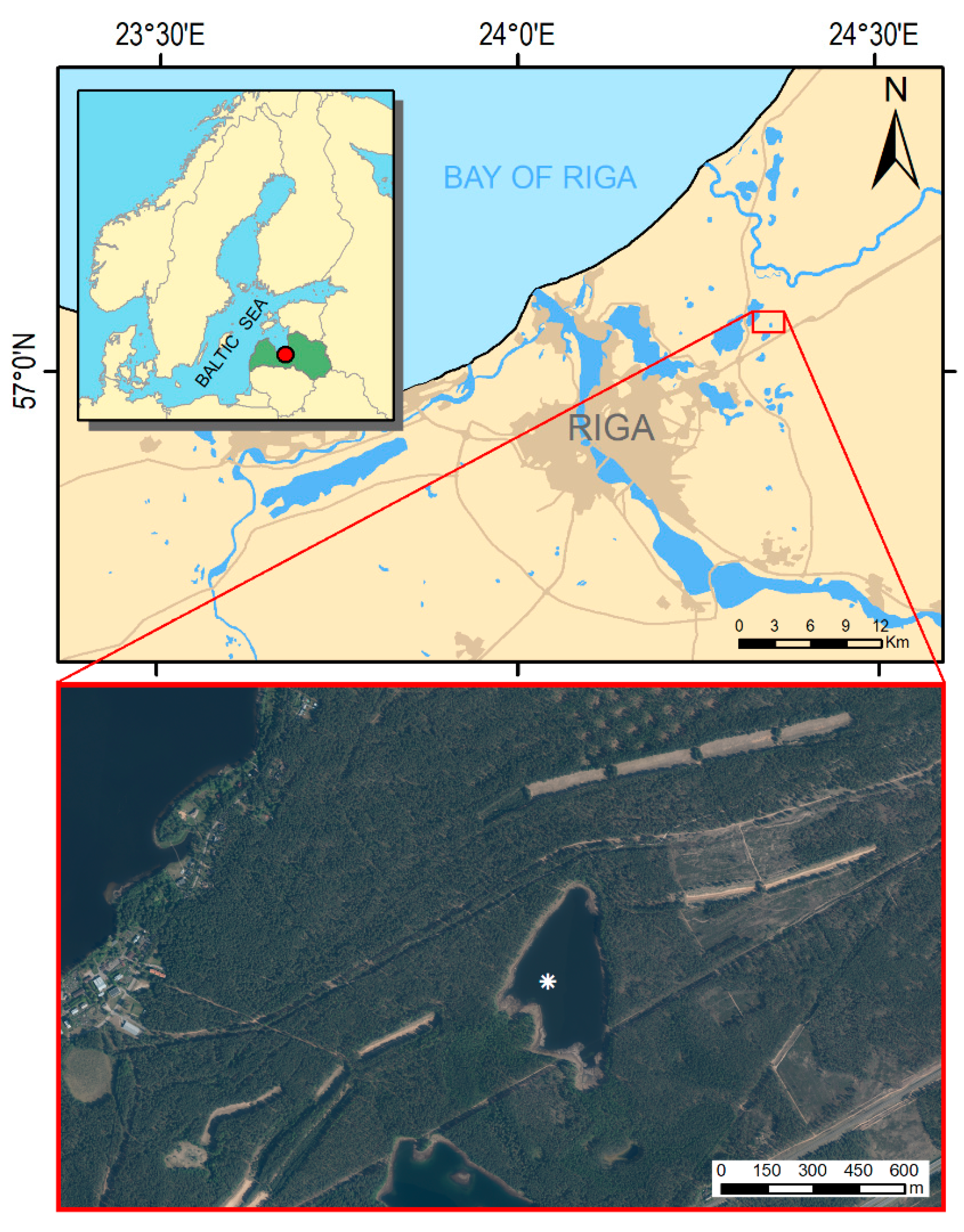
2.1. Study Site
2.2. Materials and Methods
2.2.1. Lake Sediment Coring
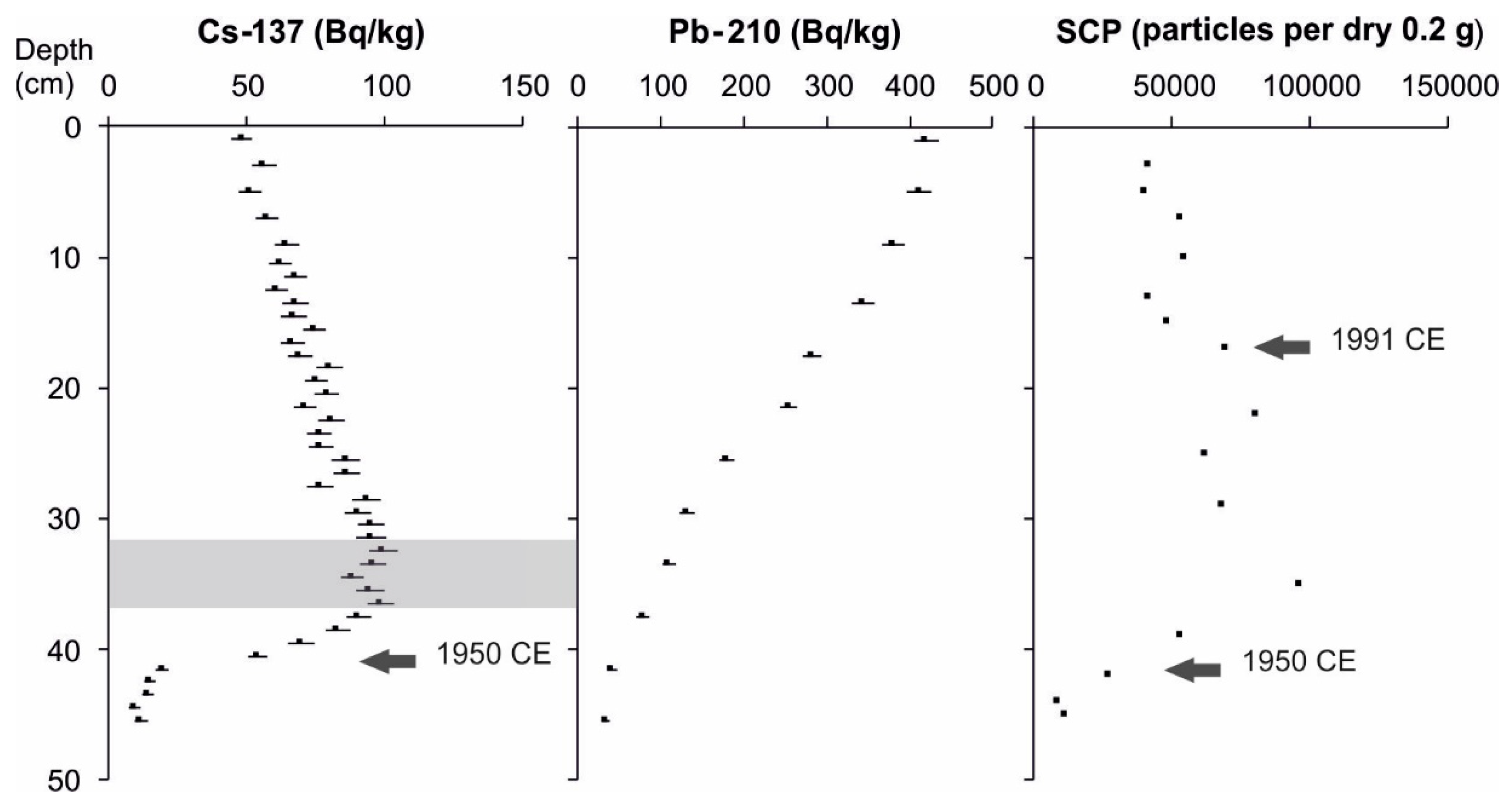
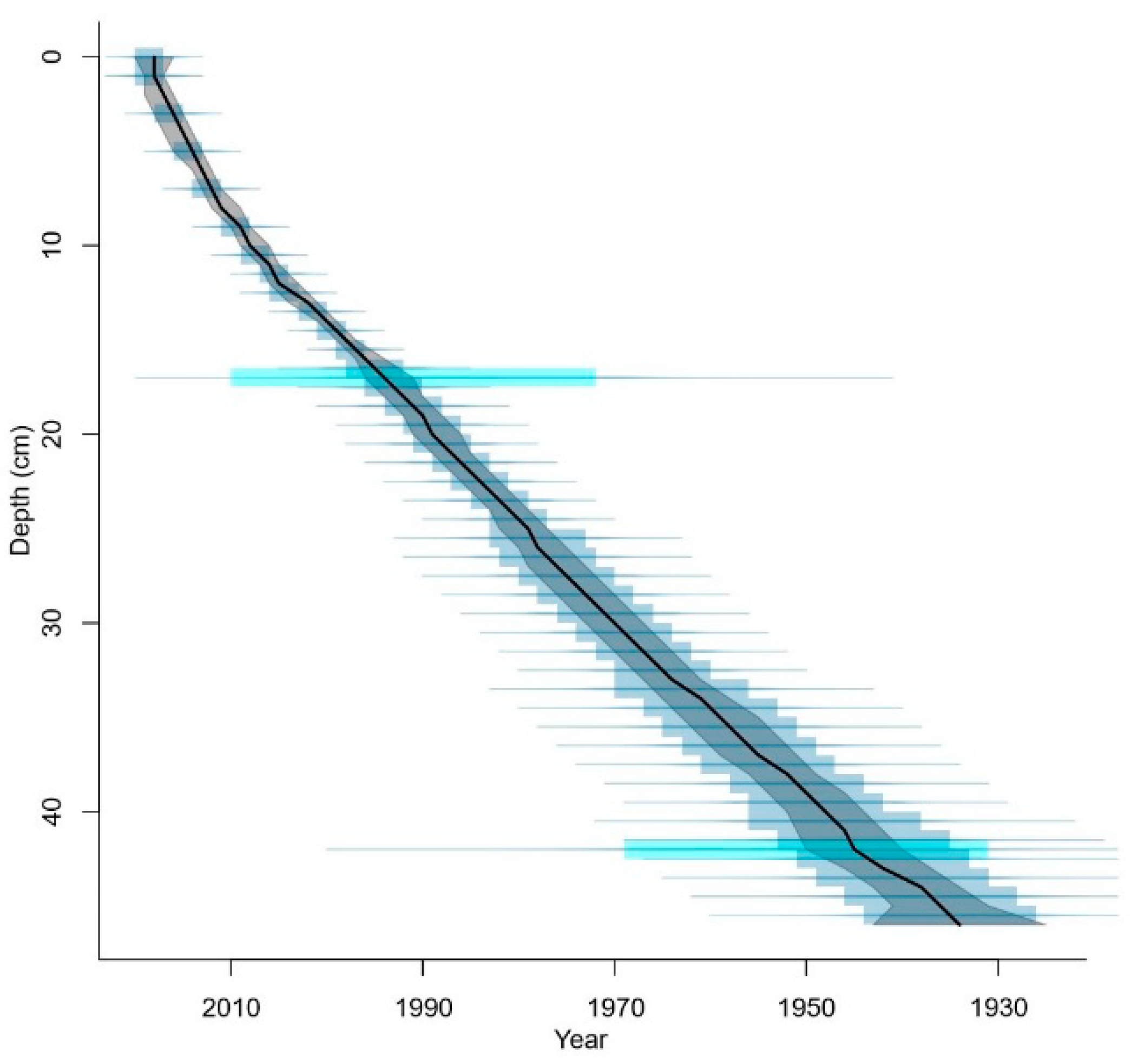
2.2.2. Core Chronology
2.2.3. Physical and Chemical Sediment Analyses
2.2.4. Pollen and Non-Pollen Palynomorphs
2.2.5. Diatom Analysis
2.2.6. Cladocera Analysis
2.2.7. Chironomidae Analysis
3. Results
3.1. Core Chronology
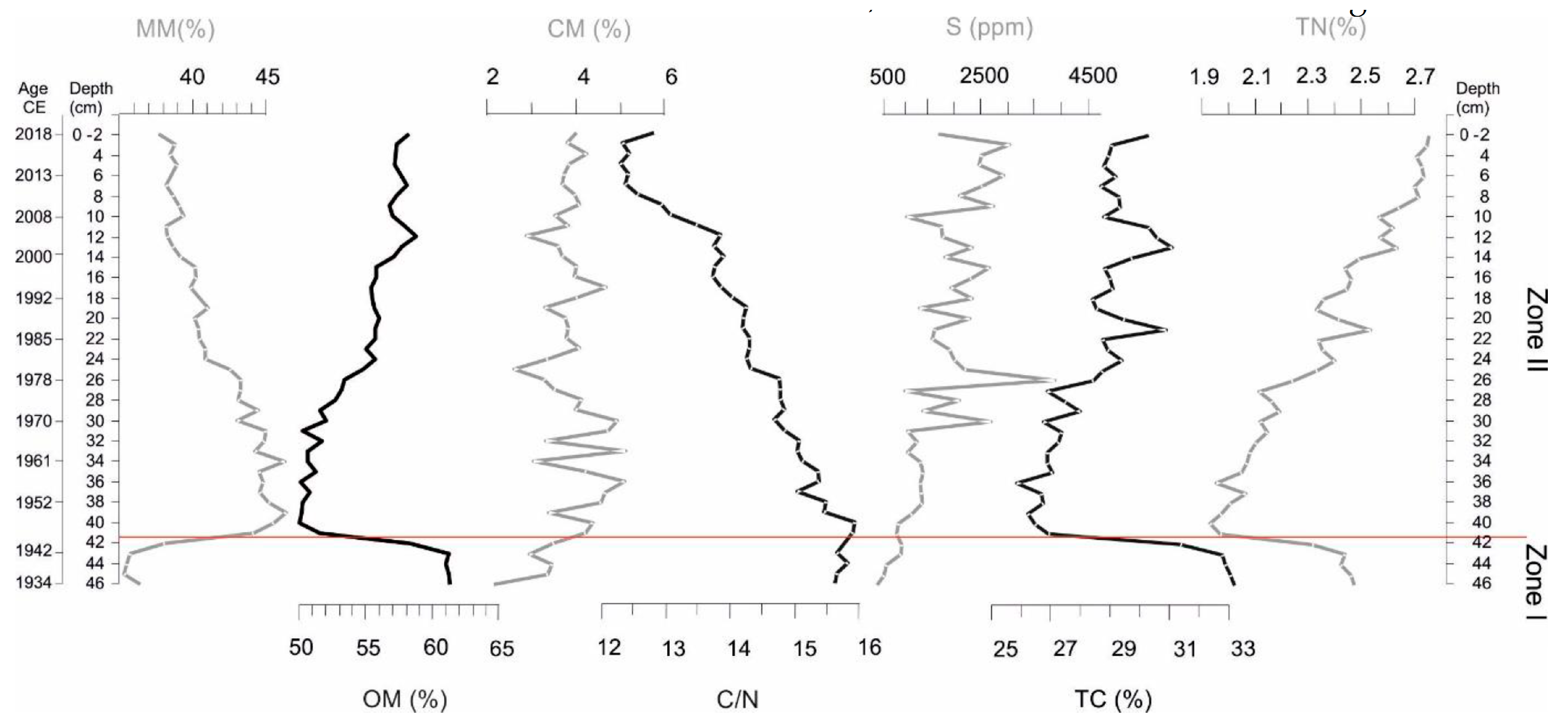
3.2. Sediment Composition
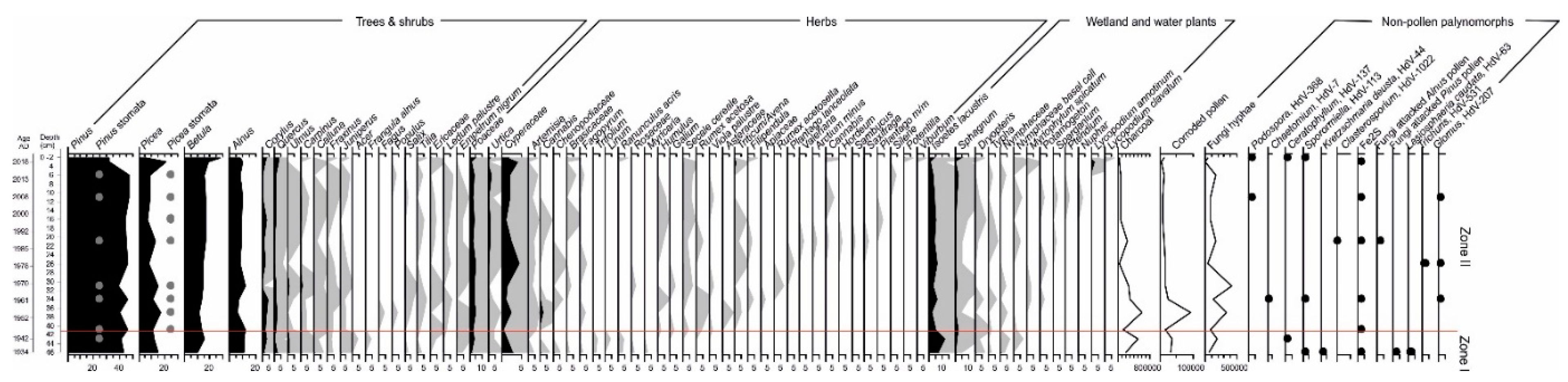
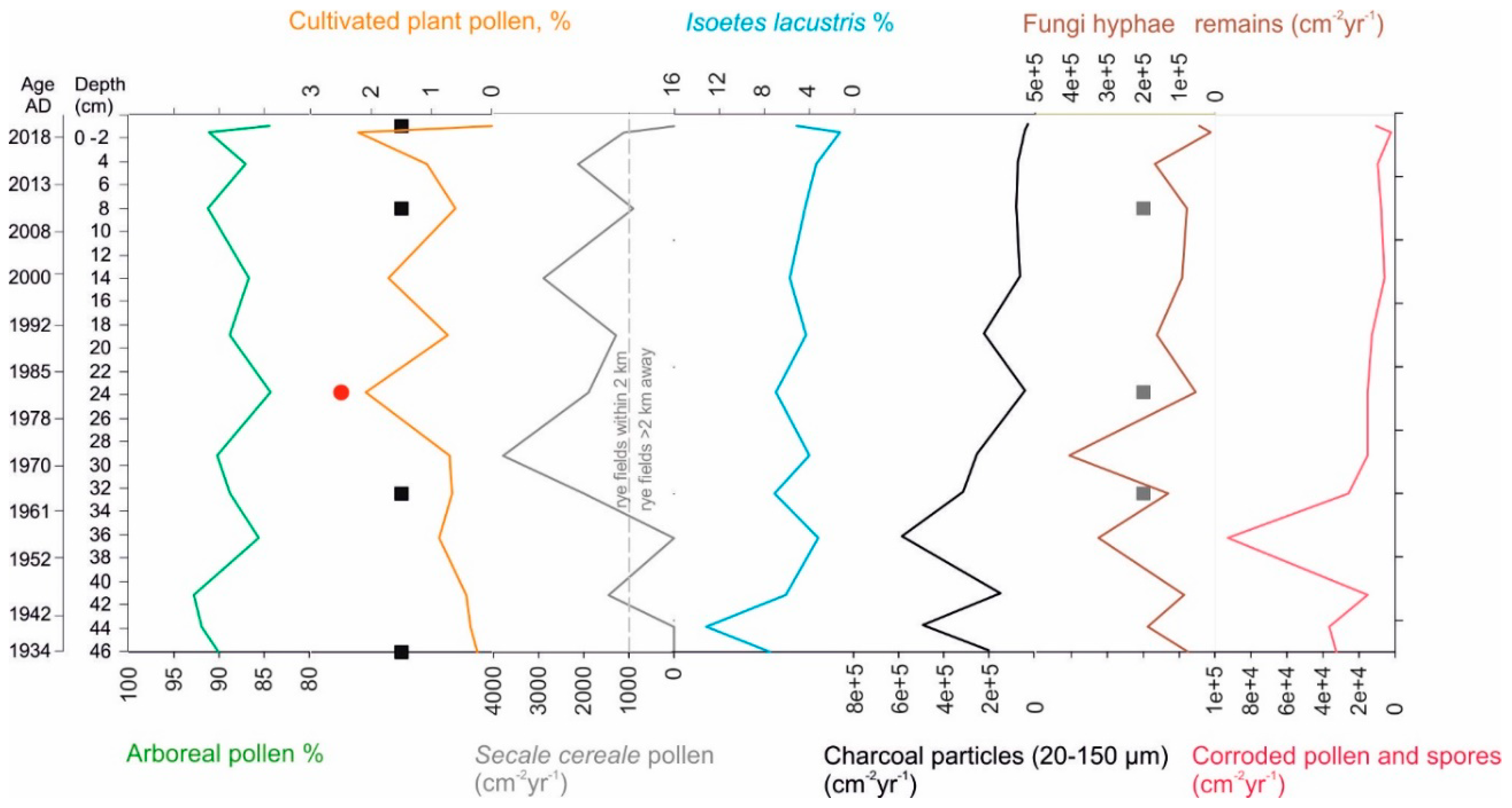
3.3. Pollen and Non-Pollen Palynomorphs
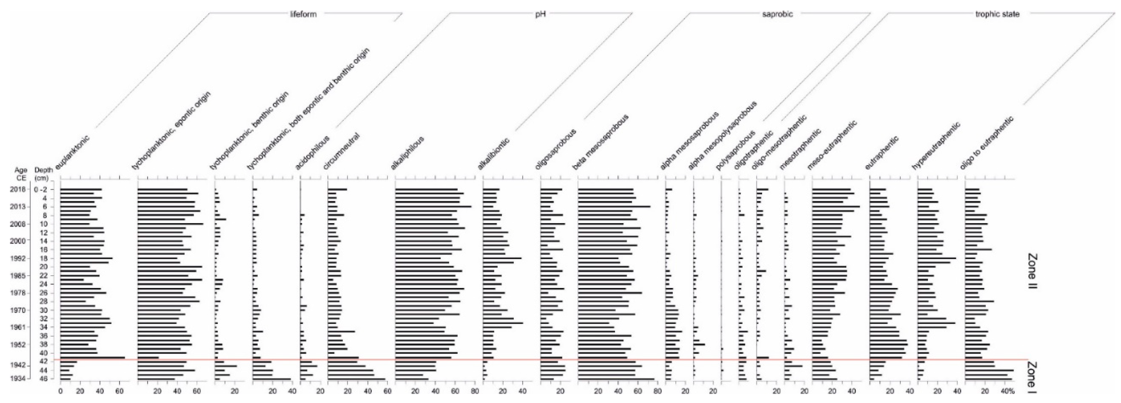
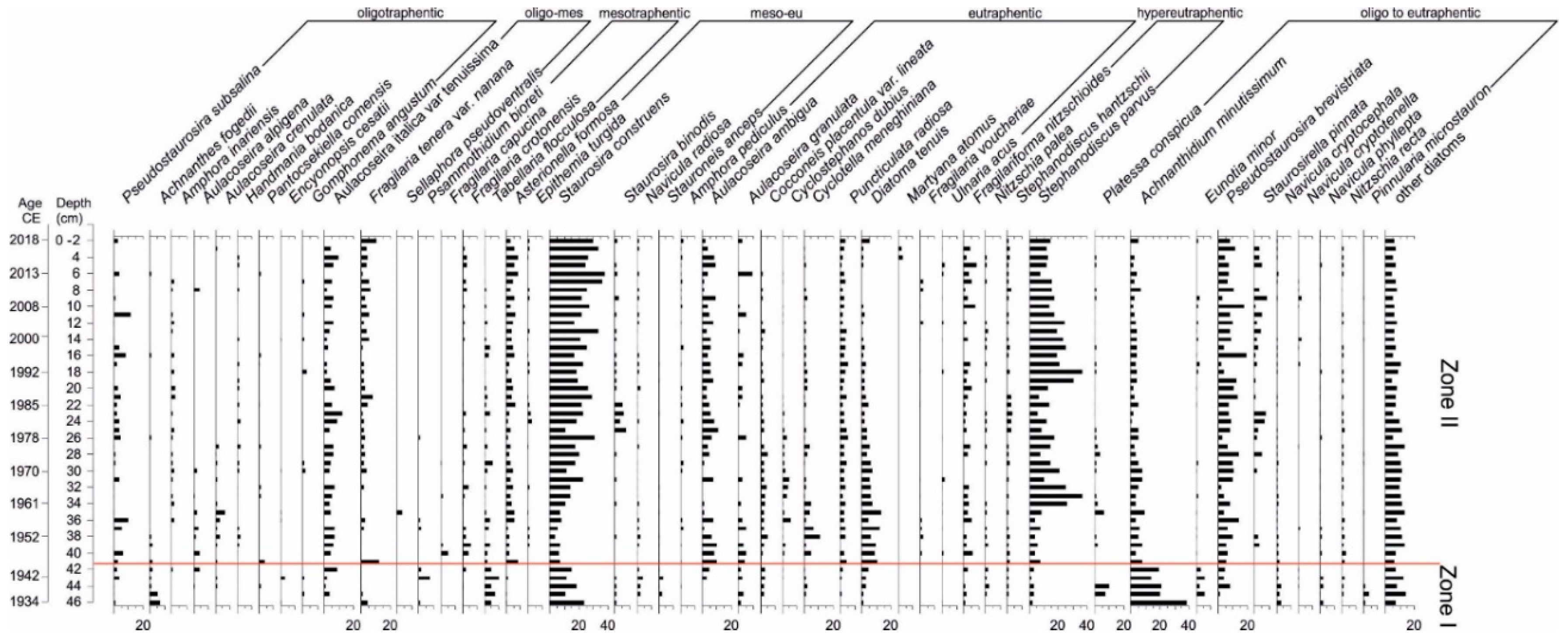
3.4. Diatom Analysis
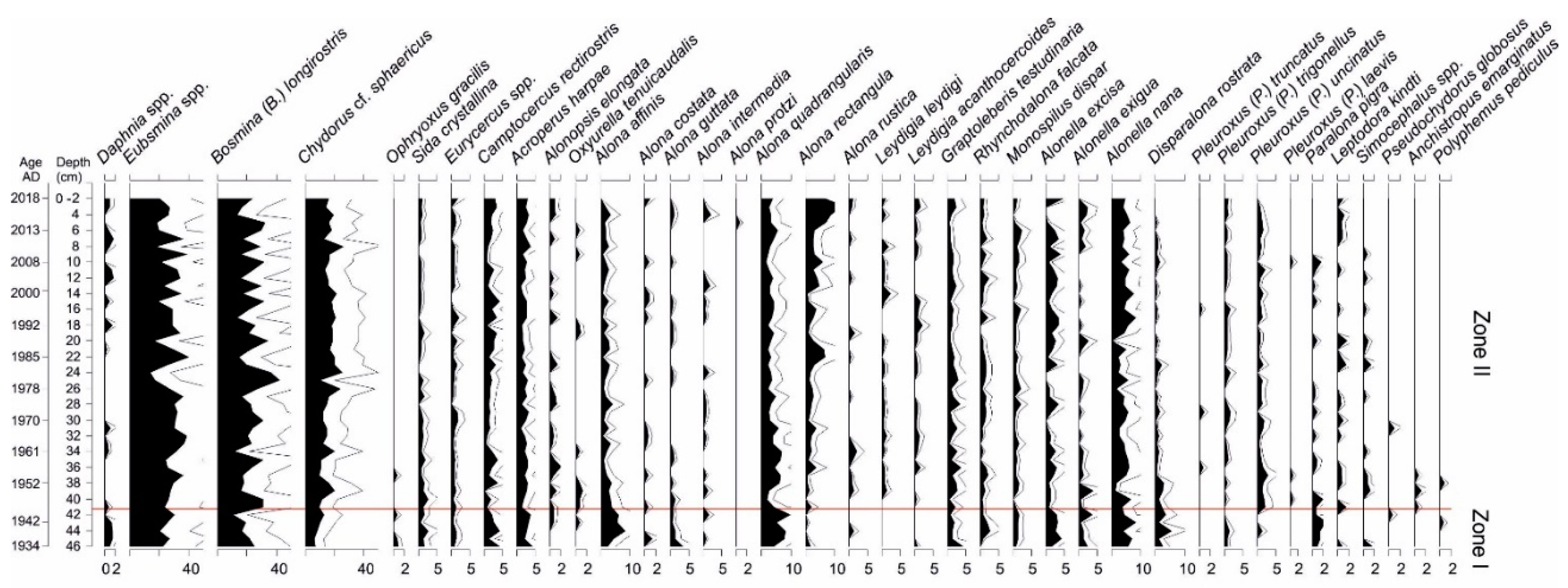
3.5. Cladocera Analysis
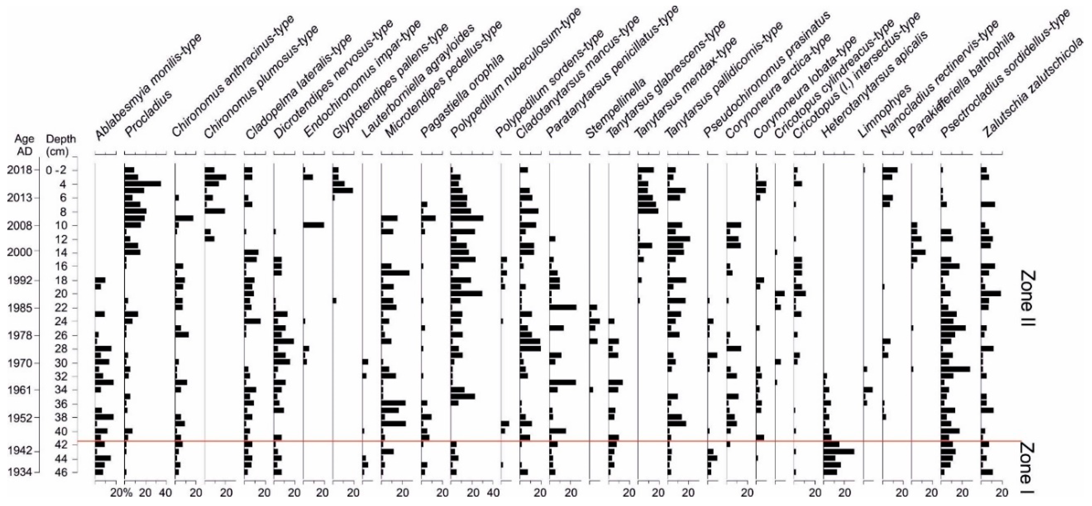
3.6. Chironomidae Analysis
4. Discussion
5. Conclusions
Author Contributions
Funding
Acknowledgments
Conflicts of Interest
References
- Haas, M.; Baumann, F.; Castella, D.; Haghipour, N.; Reusch, A.; Strasser, M.; Eglinton, T.I.; Dubois, N. Roman-driven cultural eutrophication of Lake Murten, Switzerland. Earth Planet Sci. Lett. 2019, 505, 110–117. [Google Scholar] [CrossRef]
- Wassmann, P. Cultural eutrophication: Perspectives and prospects. In Drainage Basin Nutrient Inputs and Eutrophication: An Integrated Approach; Wassmann, P., Olli, K., Eds.; University of Tromsø: Tromsø, Norway, 2005; pp. 224–234. [Google Scholar]
- Hasler, A.D. Eutrophication of lakes by domestic drainage. Ecology 1947, 28, 383–395. [Google Scholar] [CrossRef]
- Elmgren, R.; Larsson, U. Eutrophication in the Baltic Sea area: Integrated coastal management issues. In Science and Integrated Coastal Management; von Bodungen, B., Turner, R.K., Eds.; University Press: Berlin, Germany, 2001; pp. 15–35. [Google Scholar]
- Smol, J.P. Pollution of Lakes and Rivers. A Paleoenvironmental Perspective, 2nd ed.; Blackwell Publishing Ltd.: Oxford, UK, 2008; pp. 1–396. [Google Scholar]
- Yuksel, I.; Arman, H.; Ceribasi, G. Water Resources Management of Hydropower and Dams as Sustainable Development. In Proceedings of the International Conference on Sustainable Systems and the Environment (ISSE), Sharjah, UAE, 23–24 March 2011. [Google Scholar]
- Chen, J.; Qian, H.; Gao, Y.; Wang, H.; Zhang, M. Insights into hydrological and hydrochemical processes in response to water replenishment for lakes in arid regions. J. Hydrol. 2020, 581. [Google Scholar] [CrossRef]
- Dziluma, M. Riga Water and the Riga Water Supply Museum; Riga Water: Riga, Latvia, 2003; pp. 1–86. [Google Scholar]
- Jansons, E. Rīgas Dzeramais ūdens un tā Resursu Aizsardzība. Baltezeru un to Apkaimes Izpēte; Rīgas Ūdens: Rīga, Latvija, 1997; pp. 1–53. [Google Scholar]
- Krutofala, T.; Levins, I. Pazemes ūdeņu Atradnes “Baltezers”, Iecirkņa “Akoti” Pase. Pazemes ūdeņu Ekspluatācijas Krājumu Novērtējums. Atradne “Baltezers”, iecirknis “Akoti”. Gruntsūdens Horizonts; Latvijas Vides, ģeoloģijas un Meteoroloģijas Aģentūra: Rīga, Latvija, 2006; pp. 1–38. [Google Scholar]
- Pastors, A. Sekšu ezers. In Latvijas Daba: Enciklopēdija; Kavacs, G., Ed.; Latvijas Enciklopēdija: Rīga, Latvija, 1995; Volume 5, pp. 12–13. [Google Scholar]
- Bauze-Krastiņš, M.G. Garkalnes novada teritorijas plānojums 2009–2021. Gadam. Paskaidrojuma Raksts; Garkalnes novads: Rīga, Latvija, 2009; pp. 1–169. [Google Scholar]
- Latvijas Klimats. Latvijas Vides, ģeoloģijas un Meteoroloģijas Centrs. Available online: https://www.meteo.lv/lapas/laika-apstakli/klimatiska-informacija/latvijas-klimats/latvijas-klimats?id=1199&nid=562 (accessed on 10 March 2020).
- Natural Data Management System OAK, Meža Valsts Reģistra Informācija. Available online: http://ozols.daba.gov.lv/pub/Life/ (accessed on 10 March 2020).
- Zarina, D. Sekšu Ezera, Sudrabezera un Venču Ezera Ekoloģiskais Stāvoklis. Master’s Thesis, Latvijas Universitāte, Riga, Latvija, 2014. [Google Scholar]
- Tylmann, W.; Bonk, A.; Goslar, T.; Wulf, S.; Grosjean, M. Calibrating 210Pb dating results with varve chronology and independent chronostratigraphic markers: Problems and implications. Quat. Geochronol. 2016, 32, 1–10. [Google Scholar] [CrossRef] [Green Version]
- Rose, N. A method for the selective removal of inorganic ash particles from lake sediments. J. Paleolimnol. 1990, 4, 61–68. [Google Scholar] [CrossRef]
- Alliksaar, T. Spatial and temporal variability of the distribution of spherical fly-ash particles in sediments in Estonia. Ph.D. Thesis, Tallinn Pedagogical University, Tallinn, Estonia, 2000. [Google Scholar]
- Hedges, J.I.; Eglinton, G.; Hatcher, P.G.; Kirchman, D.L.; Arnosti, C.; Derenne, S.; Evershed, R.P.; Kögel-Knabner, I.; de Leeuw, J.W.; Littke, R.; et al. The molecularly-uncharacterized component of non-living organic matter in natural environments. Org. Geochem. 2000, 31, 945–958. [Google Scholar] [CrossRef]
- Masiello, C.A. New directions in black carbon organic geochemistry. Mar. Chem. 2004, 92, 201–213. [Google Scholar] [CrossRef]
- Stivrins, N.; Wulf, S.; Wastegård, S.; Lind, E.M.; Allisaar, T.; Gałka, M.; Andersen, T.J.; Heinsalu, A.; Seppä, H.; Veski, S. Detection of the Askja AD 1875 cryptotephra in Latvia, Eastern Europe. J. Quat. Sci. 2016, 31, 437–441. [Google Scholar] [CrossRef] [Green Version]
- Blaauw, M. Methods and code for ‘classical’ age-modelling of radiocarbon sequences. Quat. Geochronol. 2010, 5, 512–518. [Google Scholar] [CrossRef]
- R Core Team. R: A Language and Environment for Statistical Computing; R Foundation: Vienna, Austria, 2018. [Google Scholar]
- Heiri, O.; Lotter, A.F.; Lemcke, G. Loss on ignition as a method for estimating organic and carbonate content in sediments, reproducibility and comparability of results. J. Paleolimnol. 2001, 25, 101–110. [Google Scholar] [CrossRef]
- Berglund, B.E.; Ralska-Jasiewiczowa, M. Pollen analysis and pollen diagrams. In Handbook of Holocene Palaeoecology and Palaeohydrology; Berglund, B., Ed.; John Wiley & Sons: Chichester, UK, 1986; pp. 455–484. [Google Scholar]
- Stockmarr, J. Tablets with spores used in absolute pollen analysis. Pollen Spores 1971, 13, 615–621. [Google Scholar]
- Fægri, K.; Iversen, J. Textbook of Pollen Analysis; John Wiley & Sons: Chichester, UK, 1986. [Google Scholar]
- Miola, A. Tools for non-pollen palynomorphs (NPPs) analysis: A list of quaternary NPP types and reference literature in English language (1972–2011). Rev. Palaeobot. Palynol. 2012, 186, 142–161. [Google Scholar] [CrossRef]
- Sweeney, C.A. A key for the identification of stomata of the native conifers of Scandinavia. Rev. Palaeobot. Palynol. 2004, 128, 281–290. [Google Scholar] [CrossRef]
- Finsinger, W.; Tinner, W. New insights on stomata analysis of European conifers 65 years after the pioneering study of Werner Trautmann (1953). Veg. Hist. Archaeobotany 2019. [Google Scholar] [CrossRef]
- Grimm, E.C. TILIA Software; Illinois State Museum, Research and Collection Center: Springfield, IL, USA, 2012. [Google Scholar]
- Battarbee, R.W. Diatom analysis. In Handbook of Holocene Paleoecology and Paleohydrology; Berglund, B.E., Ed.; John Wiley and Sons Ltd.: Chichester, UK, 1986; pp. 527–570. [Google Scholar]
- Battarbee, R.W.; Kneen, M.J. The use of electronically counted microsphere sin absolute diatom analysis. Limnol. Oceanogr. 1982, 27, 184–188. [Google Scholar] [CrossRef]
- Krammer, K.; Lange-Bertalot, H. Bacillariophyceae 4. Achnanthaceae. In Süsswasserflora von Mitteleuropa, 3rd ed.; Ettl, H., Gärtner, G., Gerloff, J., Heyning, H., Mollenhauer, D., Eds.; Fisher: Stuttgardt, Germany, 2011; Volume 2, p. 437. [Google Scholar]
- Krammer, K.; Lange-Bertalot, H. Bacillariophyceae 1. Naviculaceae. In Süsswasserflora von Mitteleuropa, 4th ed.; Ettl, H., Gerloff, J., Heyning, H., Mollenhauer, D., Eds.; Fisher: Stuttgardt, Germany, 2010; Volume 2, p. 876. [Google Scholar]
- Krammer, K.; Lange-Bertalot, H. Bacillariophyceae 2. Ephitemiaceae. Bacillariaceae. Surirellaceae. In Süsswasserflora von Mitteleuropa, 4th ed.; Ettl, H., Gerloff, J., Heyning, H., Mollenhauer, D., Eds.; Fisher: Stuttgardt, Germany, 2008; Volume 2, p. 596. [Google Scholar]
- Krammer, K.; Lange-Bertalot, H. Bacillariophyceae 3. Centrales. Fragilariaceae. Eunotiaceae. In Süsswasserflora von Mitteleuropa, 3rd ed.; Ettl, H., Gerloff, J., Heyning, H., Mollenhauer, D., Eds.; Fisher: Stuttgardt, Germany, 2008; Volume 2, pp. 1–577. [Google Scholar]
- Lange-Bertalot, H.; Hofmann, G.; Werum, M. Diatomeen im Süßwasser-Benthos von Mitteleuropa; A.R.G. Gantner Verlag, K.G.: Ruggell, Liechtenstein, 2011; pp. 1–908. [Google Scholar]
- Lange-Bertalot, H.; Metzeltin, D. Indicators of Oligotrophy. 800 taxa representative of three ecologically distinct lake types. In Iconographia Diatomologica: Annotated Diatom Micrographs; Lange-Bertalot, H., Ed.; A.R.G. Gantner Verlag, K.G.: Ruggel, Liechtenstein, 1996; pp. 1–390. [Google Scholar]
- Lange-Bertalot, H.; Bąk, M.; Witkowski, A.; Tagliaventi, N. Eunotia and related genera. In Diatoms of Europe; A.R.G. Gantner Verlag, K.G.: Ruggell, Liechtenstein, 2011; Volume 6, pp. 1–747. [Google Scholar]
- AlgaeBase. Available online: https://www.algaebase.org/ (accessed on 19 February 2020).
- Lecointe, C.; Coste, M.; Prygiel, J. “Omnidia”: Software for taxonomy, calculation of diatom indices and inventories management. In Twelfth International Diatom Symposium; Springer: Dordrecht, The Netherlands, 1993; pp. 509–513. [Google Scholar]
- Denys, L. A Check-List of the Diatoms in the Holocene Deposits of the Western Belgian Coastal Plain with a Survey of their Apparent Ecological Requirements; Service Geologique de Belgique: Brussels, Belgium, 1991; Volume 1, pp. 1–2. [Google Scholar]
- Van Dam, H.; Mertens, A.; Sinkeldam, J. A coded checklist and ecological indicator values of freshwater diatoms from the Netherlands. Neth. J. Aquat. Ecol. 1994, 28, 117–133. [Google Scholar]
- Juggins, S. Version 1.0. User Guide. The European Diatom Database; Newcastle University: Newcastle upon Tyne, UK, 2001. [Google Scholar]
- Szeroczyńska, K.; Sarmaja-Korjonen, K. Atlas of Subfossil Cladocera from Central and Northern Europe; Friends of Lower Vistula Society: Świecie, Poland, 2007; pp. 1–84. [Google Scholar]
- Kurek, J.; Korosi, J.B.; Jeziorski, A.; Smol, J.P. Establishing reliable minimum count sizes for cladoceran subfossils sampled from lake sediments. J. Paleolimnol. 2010, 44, 603–612. [Google Scholar] [CrossRef]
- Juggins, S. C2 Version 1.5. User Guide. Software for Ecological and Palaeoecological Data Analysis and Visualisation; Newcastle University: Newcastle upon Tyne, UK, 2007. [Google Scholar]
- Flössner, D. Die Haplopoda und Cladocera (ohne Bosminidae) Mitteleuropas; Backhuys Publishers: Leiden, The Netherlands, 2000; p. 428. [Google Scholar]
- Brooks, S.J.; Langdon, P.G.; Heiri, O. The Identification and Use of Palaearctic Chironomidae Larvae in Palaeoecology; Quaternary Research Association: Edinburgh, UK, 2007. [Google Scholar]
- Luoto, T.P.; Nevalainen, L. Inferring reference conditions of hypolimnetic oxygen for deteriorated Lake Mallusjärvi in the cultural landscape of Mallusjoki, southern Finland using fossil midge assemblages. Water Air Soil Pollut. 2011, 217, 663–675. [Google Scholar] [CrossRef]
- Luoto, T.P.; Salonen, V.P. Fossil midge larvae (Diptera: Chironomidae) as quantitative indicators of late-winter hypolimnetic oxygen in southern Finland: A calibration model, case studies and potentialities. Boreal Environ. Res. 2010, 15, 1–18. [Google Scholar]
- Meltsov, V.; Poska, A.; Odgaardd, B.V.; Sammula, M.; Kull, T. Palynological richness and pollen sample evenness in relation to local floristic diversity in southern Estonia. Rev. Palaeobot. Palynol. 2011, 166, 344–351. [Google Scholar] [CrossRef]
- Stivrins, N.; Kołaczek, P.; Reitalu, T.; Seppä, H.; Veski, S. Phytoplankton response to the environmental and climatic variability in a temperate lake over the last 14,500 years in eastern Latvia. J. Paleolimnol. 2015, 54, 103–119. [Google Scholar] [CrossRef]
- Schindler, D.W. The Dilemma of Controlling Cultural Eutrophication of Lakes. Proc. R. Soc. B 2012, 279, 4322–4333. [Google Scholar] [CrossRef] [PubMed] [Green Version]
- Lampert, W.; Sommer, U. Limnoecology; Oxford University Press: Oxford, UK, 1997; pp. 1–382. [Google Scholar]
- Schindler, D.W. Recent advances in the understanding and management of eutrophication. Limnol. Oceanogr. 2006, 51, 356–363. [Google Scholar] [CrossRef] [Green Version]
- Leira, M.; Cantonati, M. Effects of water-level fluctuations on lakes: An annotated bibliography. Hydrobiologia 2008, 613, 171–184. [Google Scholar] [CrossRef]
- Koralay, N.; Kara, O. Effects of Soil Erosion on Water Quality and Aquatic Ecosystem in a Watershed. In Proceedings of the 1st International Congress on Agricultural Structures and Irrigation, Antalya, Turkey, 26–28 September 2018; pp. 20–29. [Google Scholar]
- Kuptsch, P. Die Cladoceren der Umgegend von Riga. Arch. Hydrobiol. 1927, 18, 273–315. [Google Scholar]
- Hakkari, L. Zooplankton species as indicators of environment. Aqua Fenn. 1972, 1, 46–54. [Google Scholar]
- Lyche, A. Cluster analysis of plankton community structure in 21 lakes along a gradient of trophy. Verh. Internat. Verein Limnol. 1990, 24, 586–591. [Google Scholar] [CrossRef]
- Urtane, L. Cladocera as indicators of lake types and trophic state in Latvian lakes. Ph.D. Thesis, University of Latvia, Riga, Latvia, 1998. [Google Scholar]
- Walseng, B.; Halvorsen, G. Littoral microcrustaceans as indices of trophy. Verh. Internat. Verein Limnol. 2005, 29, 827–829. [Google Scholar] [CrossRef]
- Jensen, T.C.; Dimante-Deimantovica, I.; Schartau, A.K.; Walseng, B. Cladocerans respond to differences in trophic state in deeper nutrient poor lakes from Southern Norway. Hydrobiologia 2013, 715, 101–112. [Google Scholar] [CrossRef]
- Umja Ezera Dabas Aizsardzības Plāns. Available online: https://www.daba.gov.lv/upload/File/DAPi_apstiprin/DL_Ummis-06.pdf (accessed on 20 March 2020).
- Susko, U.; Latvian Fund for Nature, Riga, Latvia. Personal communication, 2020.
- Sloka, N. Latvijas PSR Dzīvnieku Noteicējs. Latvijas Kladoceru (Cladocera) Fauna un Noteicējs; P. Stučkas Latvijas valsts universitāte: Rīga, Latvia, 1981; p. 146. [Google Scholar]
- Eutrophication of Waters, Monitoring, Assessment and Control; OECD (Organisation for Economic Cooperation and Development): Paris, France, 1982.
- Andrén, E. Changes in the Composition of the Diatom Flora During the Last Century Indicate Increased Eutrophication of the Oder Estuary, South-western Baltic Sea. Estuar. Coast. Shelf Sci. 1999, 48, 665–676. [Google Scholar] [CrossRef]
- Andrén, E.; Clarke, A.L.; Telford, R.J.; Wesckström, K.; Vilbaste, S.; Aigars, J.; Conley, D.; Johnsen, T.; Juggins, S.; Korhola, A. Defining Reference Conditions for Coastal Areas in the Baltic Sea; TemaNord Series; Nordic Council of Ministers: Copenhagen, Denmark, 2007. [Google Scholar]
- Andrén, E.; Shimmield, G.; Brand, T. Environmental changes of the last three centuries indicated by siliceous microfossil records from the southwestern Baltic Sea. Holocene 1999, 9, 25–38. [Google Scholar] [CrossRef]
- Weckström, K. Assessing recent eutrophication in coastal waters of the Gulf of Finland (Baltic Sea) using subfossil diatoms. J. Paleolimnol. 2006, 35, 571–592. [Google Scholar] [CrossRef]
- Milecka, K.; Bogaczewicz-Adamczak, B. Zmiany żyzności trofii w ekosystemach miękkowodnych jezior Borów Tucholskich. Przegl. Geol 2006, 54, 81–86. [Google Scholar]
- Christensen, K.K.; Sand-Jensen, K. Precipitated iron and manganese plaques restrict root uptake of phosphorus in Lobelia dortmanna. Can. J. Bot. 1998, 76, 2158–2163. [Google Scholar]
- Battarbee, R.W.; Simpson, G.L.; Shilland, E.M.; Flower, R.J.; Kreiser, A.; Yang, H.; Clarke, G. Recovery of UK lakes from acidification: An assessment using combined palaeoecological and contemporary diatom assemblage data. Ecol. Indic. 2014, 37, 365–380. [Google Scholar] [CrossRef]
- Battarbee, R.W.; Jones, V.J.; Flower, R.J.; Cameron, N.G.; Bennion, H.; Carvalho, L.; Juggins, S. Diatoms. In Tracking Environmental Change Using Lake Sediments. Terrestrial, Algal, and Siliceous Indicators; Smol, J.P., Birks, H.J.B., Last, W.M., Eds.; Kluwier Academic Publishers: Norwell, MA, USA, 2001; Volume 3, pp. 155–202. [Google Scholar]
- Battarbee, R.W.; Charles, D.F.; Dixit, S.S.; Renberg, I. Diatoms as indicators of surface water acidity. In The Diatoms: Applications for the Environmental and Earth Sciences; Stoermer, E.F., Smol, J.P., Eds.; Cambridge University Press: Cambridge, UK, 1999; pp. 85–127. [Google Scholar]
- Battarbee, R.W.; Charles, D.F. Diatom-based pH reconstruction studies of acid lakes in Europe and North America: A synthesis. Water Air Soil Pollut. 1986, 30, 347–354. [Google Scholar] [CrossRef]
- Klavins, M.; Kokorite, I.; Jankevica, M.; Mazeika, J.; Rodinov, V. Trace elements in sediments of lakes in Latvia. In Proceedings of the 4th WSEAS International Conference on Energy and Development—Environment—Biomedicine, Corfu Island, Greece, 14–16 July 2011. [Google Scholar]
- Kļaviņš, M.; Briede, A.; Kļaviņa, I.; Rodinov, V. Metals in sediments of lakes in Latvia. Environ. Int. 1995, 21, 451–458. [Google Scholar] [CrossRef]
- Liiv, M.; Alliksaar, T.; Amon, L.; Freiberg, R.; Heinsalu, A.; Reitalu, T.; Saarse, L.; Seppä, H.; Stivrins, N.; Tõnno, I.; et al. Late glacial and early Holocene climate and environmental changes in the eastern Baltic area inferred from sediment C/N ratio. J. Paleolimnol. 2019, 61, 1–16. [Google Scholar] [CrossRef]
- Terasmaa, J.; Puusepp, L.; Marzecová, A.; Vandel, E.; Vaasma, T.; Koff, T. Natural and human-induced environmental changes in Eastern Europe during the Holocene: A multi-proxy palaeolimnological study of a small Latvian lake in a humid temperate zone. J. Paleolimnol. 2013, 49, 663–678. [Google Scholar] [CrossRef]
- Meyers, P.A.; Ishiwatari, R. Lacustrine organic geochemistry—An overview of indicators of organic matter sources and diagenesis in lake sediments. Org. Geochem. 1993, 20, 867–900. [Google Scholar] [CrossRef] [Green Version]
- Meyers, P.A.; Teranes, J.L. Sediment Organic Matter. In Tracking Environmental Change Using Lake Sediments: Physical and Geochemical Methods, Developments in Paleoenvironmental Research; Last, W.M., Smol, J.P., Eds.; Springer: Dordrecht, The Netherlands, 2001; pp. 239–269. [Google Scholar]
- Buzajevs, V.; Levina, N.; Levins, I. Pazemes ūdeņu bilance un kvalitāte Baltezera ūdensgūtnēs; Valsts Ģeoloģijas Dienests: Riga, Latvia, 1997; pp. 1–56. [Google Scholar]
- Sarmaja-Korjonen, K. Correlation of fluctuations in cladoceran planktonic: Littoral ratio between three cores from a small lake in southern Finland: Holocene water-level changes. Holocene 2001, 11, 53–63. [Google Scholar] [CrossRef]
- Cooper, J.T.; Steinitz-Kannan, M.; Kallmeyer, D.E. Bacillariophyta: The Diatoms. In Algae: Source of Treatment; Ripley, M.G., Ed.; American Water Works Association: Denver, CO, USA, 2010; pp. 207–215. [Google Scholar]
- Zelnik, I.; Balanč, T.; Toman, M. Diversity and Structure of the Tychoplankton Diatom Community in the Limnocrene Spring Zelenci (Slovenia) in Relation to Environmental Factors. Water 2018, 10, 361. [Google Scholar] [CrossRef] [Green Version]
- Dimante-Deimantovica, I.; Latvian Institute of Aquatic Ecology, Riga, Latvia. Personal communication, 2020.
- Ardiles, V.; Alcocer, J.; Vilaclara, G.; Oseguera, L.A.; Velasco, L. Diatom fluxes in a tropical, oligotrophic lake dominated by large-sized phytoplankton. Hydrobiologia 2012, 679, 77–90. [Google Scholar] [CrossRef]
- Romero, O.E.; Thunell, R.C.; Astor, Y.; Varela, R. Seasonal and interannual dynamics in diatom production in the Cariaco Basin, Venezuela. Deep-Sea Res. 2009, 56, 571–581. [Google Scholar] [CrossRef]
- Ryves, D.B.; Jewson, D.H.; Sturm, M.; Battarbee, R.W.; Flower, R.J.; Mackay, A.W.; Granin, N.G. Quantitative and qualitative relationships between planktonic diatom communities and diatom assemblages in sedimenting material and surface sediments in Lake Baikal, Siberia. Limnol. Oceanogr. 2003, 48, 1643–1661. [Google Scholar] [CrossRef] [Green Version]
- Ceirans, A. Zooplankton indicators of trophy in Latvian lakes. In Acta Universitatis Latviensis. Biology; University of Latvia: Riga, Latvia, 2007; Volume 723, pp. 61–69. [Google Scholar]
- Veski, S.; Amon, L.; Heinsalu, A.; Reitalu, T.; Saarse, L.; Stivrins, N.; Vassiljev, J. Lateglacial vegetation dynamics in the eastern Baltic region between 14,500 and 11,400 cal yr BP: A complete record since the Bolling (GI-1e) to the Holocene. Quat. Sci. Rev. 2012, 40, 39–53. [Google Scholar] [CrossRef]
- Kołaczek, P.; Zubek, S.; Błaszkowski, J.; Mleczko, P.; Włodzimierz, M. Erosion or plant succession—How to interpret the presence of arbuscular mycorrhizal fungi (Glomeromycota) spores in pollen profiles collected from mires. Rev. Palaeobot. Palynol. 2013, 189, 29–37. [Google Scholar] [CrossRef]
- Wang, L.; Mackay, A.W.; Leng, M.J.; Rioual, P.; Panizzo, V.N.; Lu, H.; Gu, Z.; Chu, G.; Han, J.; Kendrick, C.P. Influence of the ratio of planktonic to benthic diatoms on lacustrine organic matter δ13C from Erlongwan maar lake, northeast China. Org. Geochem. 2013, 54, 62–68. [Google Scholar] [CrossRef] [Green Version]
- Wolin, J.A.; Stone, J.R. Diatoms as Indicators of Water-Level Change in Freshwater Lakes. In The Diatoms Applications to the Environmental and Earth Sciences; Stoermer, E.F., Smol, J.P., Eds.; Cambridge University Press: Cambridge, UK, 2010; pp. 174–185. [Google Scholar]
- Carmignani, J.R.; Roy, A.H. Ecological impacts of winter water level drawdowns on lake littoral zones: A review. Aquat. Sci. 2017, 79, 803–824. [Google Scholar] [CrossRef] [Green Version]
- Magny, M.; Arnaud, F.; Billaud, Y.; Marguet, A. Lake-level fluctuations at Lake Bourget (eastern France) around 4500–3500 cal. a BP and their palaeoclimatic and archaeological implications. J. Quat. Sci. 2012, 27, 494–502. [Google Scholar] [CrossRef]
- Theuerkauf, E.J.; Braun, K.N.; Nelson, D.M.; Kaplan, M.; Vivirito, S.; Williams, J.D. Coastal geomorphic response to seasonal water-level rise in the Laurentian Great Lakes: An example from Illinois Beach State Park, USA. J. Great Lakes Res. 2019, 45, 1055–1068. [Google Scholar] [CrossRef]
- Holmer, M.; Storkholm, P. Sulphate reduction and sulphur cycling in lake sediments: A review. Freshw. Biol. 2001, 46, 431–451. [Google Scholar] [CrossRef]
- Couture, R.M.; Fischer, R.; Van Cappellen, P.; Gobeil, C. Non-steady state diagenesis of organic and inorganic sulfur in lake sediments. Geochim. Cosmochim. Acta 2016, 194, 15–33. [Google Scholar] [CrossRef] [Green Version]
- Aasif, A.; Nilli, A.; Aasif, L.; Hema, A.; Rayees, S. Diatom Diversity and Organic Matter Sources in Water Bodies around Chennai, Tamil Nadu, India. MOJ Ecol. Environ. Sci. 2017, 2, 141–146. [Google Scholar]
- Rosińska, A.; Rakocz, K. Rola biodegradowalnej materii organicznej w procesie dezynfekcji wody. Inż. Ochr. Środ. 2013, 16, 511–521. [Google Scholar]
- Brodersen, K.P.; Quinlan, R. Midges as palaeoindicators of lake productivity, eutrophication and hypolimnetic oxygen. Quat. Sci. 2006, 25, 1995–2012. [Google Scholar] [CrossRef]
- Timrots, P.; Riga Water Supply Museum, Riga, Latvia. Personal communication, 2019.
- Brodersen, K.P.; Pedersen, O.; Lindegaard, C.; Hamburger, K. Chironomids (Diptera) and oxy-regulatory capacity: An experimental approach to paleolimnological interpretation. Limnol. Oceanogr. 2004, 49, 1549–1559. [Google Scholar]
- Kacalova, O.; Laganovsla, R. Zivju Barības Bāze Latvijas PSR Ezeros; Latvijas PSR Zinātņu akadēmijas izdevniecība: Rīga, Latvija, 1961; pp. 17–23. [Google Scholar]
- Bledzki, L.A.; Rybak, J.I. Freshwater Crustacean Zooplankton of Europe Cladocera and Copepoda (Calanoida, Cyclopoida), Key to Species Identification, with Notes on Ecology, Distribution, Methods and Introduction to Data Analysis; Springer: New York, NY, USA, 2016; pp. 1–918. [Google Scholar]
- Lielā un Mazā Baltezera Eitroficēšanās Izpēte. Available online: https://www.google.com/url?sa=t&rct=j&q=&esrc=s&source=web&cd=1&ved=2ahUKEwiPufXQp7_oAhXpxIsKHfMmDOcQFjAAegQIBRAB&url=https%3A%2F%2Fwww.ezeri.lv%2Fblog%2FDownloadAttachment%3Fid%3D347&usg=AOvVaw1qjWh6fVLl6-JGxc-_EbzG (accessed on 10 March 2020).
- Balode, M.; Purina, I.; Strake, S.; Purvina, S.; Pfeifere, M.; Barda, I.; Povidisa, K. Toxic cyanobacteria in the lakes located in Rīga (the capital of Latvia) and its surroundings: Present state of knowledge. Afr. J. Mar. Sci. 2006, 28, 225–230. [Google Scholar] [CrossRef]


© 2020 by the authors. Licensee MDPI, Basel, Switzerland. This article is an open access article distributed under the terms and conditions of the Creative Commons Attribution (CC BY) license (http://creativecommons.org/licenses/by/4.0/).
Share and Cite
Zawiska, I.; Dimante-Deimantovica, I.; Luoto, T.P.; Rzodkiewicz, M.; Saarni, S.; Stivrins, N.; Tylmann, W.; Lanka, A.; Robeznieks, M.; Jilbert, T. Long-Term Consequences of Water Pumping on the Ecosystem Functioning of Lake Sekšu, Latvia. Water 2020, 12, 1459. https://doi.org/10.3390/w12051459
Zawiska I, Dimante-Deimantovica I, Luoto TP, Rzodkiewicz M, Saarni S, Stivrins N, Tylmann W, Lanka A, Robeznieks M, Jilbert T. Long-Term Consequences of Water Pumping on the Ecosystem Functioning of Lake Sekšu, Latvia. Water. 2020; 12(5):1459. https://doi.org/10.3390/w12051459
Chicago/Turabian StyleZawiska, Izabela, Inta Dimante-Deimantovica, Tomi P. Luoto, Monika Rzodkiewicz, Saija Saarni, Normunds Stivrins, Wojciech Tylmann, Anna Lanka, Martins Robeznieks, and Tom Jilbert. 2020. "Long-Term Consequences of Water Pumping on the Ecosystem Functioning of Lake Sekšu, Latvia" Water 12, no. 5: 1459. https://doi.org/10.3390/w12051459