Possibility of Using Selected Rainfall-Runoff Models for Determining the Design Hydrograph in Mountainous Catchments: A Case Study in Poland

Abstract

The aim of the study was to analyze the possibility of using selected rainfall-runoff models to determine the design hydrograph and the related peak flow in a mountainous catchment. The basis for the study was the observed series of hydrometeorological data for the Grajcarek catchment area (Poland) for the years 1981–2014. The analysis was carried out in the following stages: verification of hydrometeorological data; determination of the design rainfall; and determination of runoff hydrographs with the following rainfall-runoff models: Snyder, NRCS-UH, and EBA4SUB. The conducted research allowed the conclusion that the EBA4SUB model may be an alternative to other models in determining the design hydrograph in ungauged mountainous catchments. This is evidenced by the lower values of relative errors in the estimation of peak flows with an assumed frequency for the EBA4SUB model, as compared to Snyder and NRCS-UH.

1. Introduction

Surface runoff is the amount of water that is generated when excess stormwater, meltwater, or other water sources flow over the topographic surface. It occurs, for instance, when the soil is saturated from above by infiltration, or when the soil is saturated from below by the subsurface flow. Surface runoff often occurs due to impervious areas (such as roofs and others) that do not allow water to soak into the ground. It is the primary agent of soil erosion by water [1,2]. In addition to causing soil erosion, surface runoff is a primary cause of flooding, which can result in property damages. Hence, determining the shape of design hydrographs is a very important activity in flood protection.

The knowledge of the characteristics of design hydrograph, such as peak flow, duration, or volume, is necessary for planning and designing water management facilities and determining flood risk zones. One of the methods for obtaining such information is the use of theoretical design hydrographs. These are typical hydrographs for the investigated catchment, which describe the shape of the flood wave. Hydrograph parameters are often determined on the basis of physiographic characteristics of the catchment. One particular application related to water management during floods is in uncontrolled catchments. Indeed this application is challenging because ungauged catchments’ lack of runoff measurements that are often necessary for calibrating advanced hydrological models [3,4].

There are quite a number of methods that can be used to determine design hydrographs in ungauged basins, for instance hydrological rainfall-runoff models can be used [5,6,7,8]. Of the numerous mathematical models used for the analysis of the rainfall-runoff relationship, conceptual models based on the cascade of Nash linear tanks, double cascade of tanks (Wackermann model) or synthetic unit hydrographs (Snyder, SCS-UH, Clark-UH) are commonly employed [9]. It should be emphasized that in recent years, the runoff formation in a changing environment has become an important scientific problem in hydrology. A better understanding of the runoff changes are thus of paramount importance to effectively manage water resources. The variability of hydro-meteorological conditions due to climate change significantly affects the hydrological regime in catchments [10]. Generally, climate change and human activities are significant factors influencing runoff variation [11,12]. Hence, studies related to the possibility of using new methods to determine design hydrographs should be conducted.

Past experience with the use of rainfall-runoff models has shown some limitations associated with their use. Many problems focus on the following issues: (1) Lack of guidelines for the adoption of a standard rainfall hyetograph, which increases the uncertainty of the results obtained; (2) High sensitivity of synthetic hydrographs to the distribution of rainfall patterns in the catchment and rainfall height measurement errors; (3) Overestimation or underestimation of direct runoff from the original SCS-CN method; (4) Uncertainty of the results of SCS-UH in relation to the input parameters; (5) Subjectivity of the selection of the size of the indicators for estimating the parameters of selected models [13,14,15,16]. An alternative to the rainfall-runoff models used so far may be the recently developed “Event-based Approach for Small and Ungauged Basins” (EBA4SUB) model. It allows estimating the magnitude of the peak flow along with the characteristics of the design hydrograph (e.g., duration and volume). This model has been fully adapted to determine the floods in uncontrolled catchments. It is based on geographic information systems and on the optimization of topographic information contained in the digital elevation model. The EBA4SUB model was developed to obtain the design hydrograph with the smallest possible input information like when using the well-known rational formula [17,18,19].

Considering the limitations related to the previously aforementioned rainfall-runoff models, the overall objective of this study was a comparative analysis for the shape of design hydrograph determined in a Carpathian mountainous catchment with the following models: NRCS-UH, Snyder, and EBA4SUB. The novelties in the EBA4SUB model are in its approach towards calculating excess rainfall and its adaptation of the width function to the description of the transformation of rainfall into runoff. It should be emphasized that so far there has been no research regarding the possibility of using the EBA4SUB model to determine the design hydrographs in the Carpathian catchments. Therefore, a novelty in this study is the comparison of the EBA4SUB model with simple models commonly used in Poland, which have certain recognized limitations. The study will allow a determination as to whether the EBA4SUB model may be an alternative to commonly used methodological approaches.

2. Materials and Methods

The basis for this study was the observed time series of daily rainfall and maximum annual flows in the period 1971–2014 for the Grajcarek river, obtained from the Institute of Meteorology and Water Management in Warsaw, the National Research Institute. The analyses were carried out in the following stages: verification of hydrometeorological data, calculation of maximum annual rainfall and flows with a specified probability, determination of the design hydrographs using the analysed rainfall-runoff models described in the following, and quality assessment of the used models.

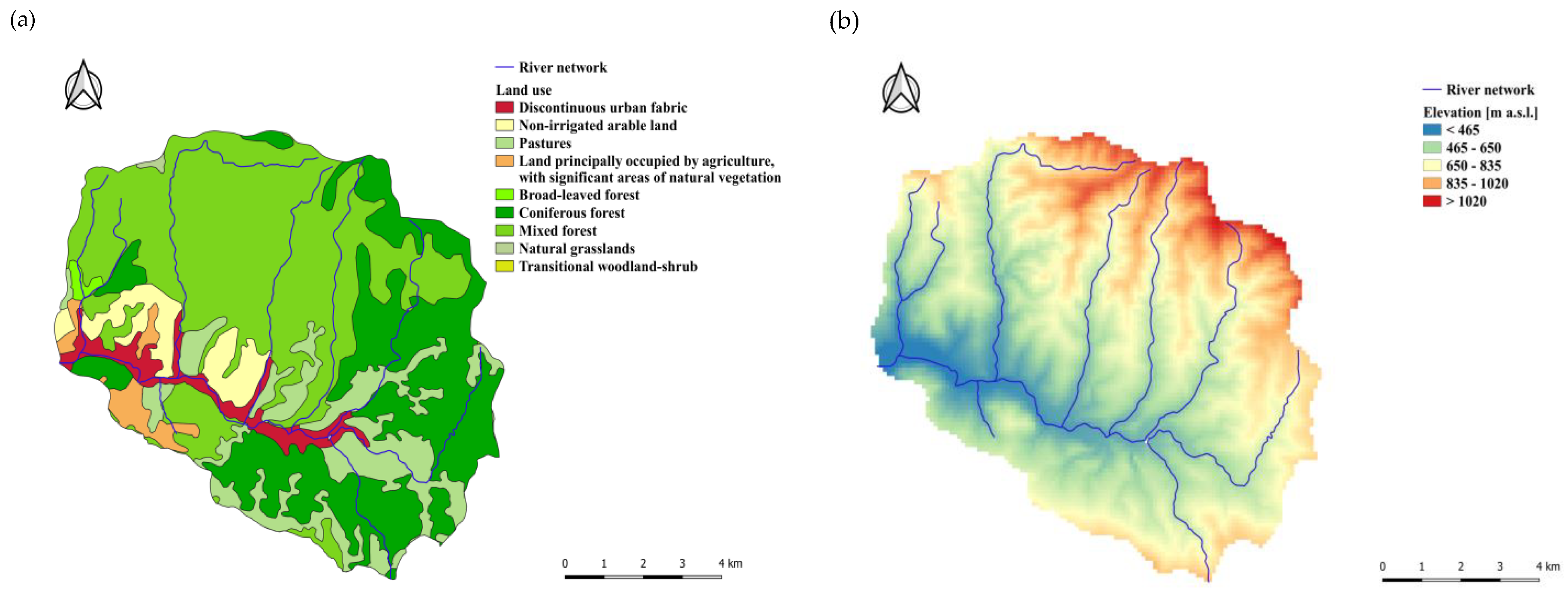
2.1. Research Area Characteristic

The selected case study is the Grajcarek river catchments (coordinates for cross-section Szczawnica: 49°25′22″ N 20°28′58″ E). It is located in the Carpathian part of the upper Vistula river catchment, in Poland. The catchment area is 86 km². The length of the main watercourse to the outlet cross-section is 15.0 km. The average catchment slope is 8%. The density of the river network is 0.70 km⁻¹. This information was derived using a Digital Elevation Model (DEM) provided by USGS—United States Geological Survey, with a grid resolution of about 25 m. Based on the Hydrographic Division Map of Poland 2010 and on the Corine Land Cover 2018 database, the following forms of land uses were identified together with the percentage of the catchment area respectively occupied. Loose urban buildings (4.5%), arable lands without irrigation (5.1%), meadows and pastures (14.4%), areas occupied mainly by agriculture with a high proportion of natural vegetation (2.1%), coniferous forests (29.8%), mixed forests (43.4%), and deciduous forests (0.2%). The case study is dominated by poorly permeable and impermeable soils. The average annual rainfall in the catchment area exceeds 765 mm. The average annual temperature is 6.8 °C. Figure 1 shows the land use and the topography of the catchment.

2.2. Hydrometeorological Data Verification

The verification of the hydrometeorological data was carried out in relation to the maximum annual daily rainfall (P_max) and the maximum annual flow (Q_max), using the Mann-Kendall test (MK). The H₀ null hypothesis of the test assumes no monotonic data trend, while the H₁ alternative states that such a trend exists. The calculations were done for the significance level α = 0.05. The S Mann-Kendall statistics were determined based on the equation [20,21]:

$$S={\Sigma }_{k=1}^{n-1}{\Sigma }_{j=k+1}^n \mathrm{sgn}(x_j - x_k)$$

(1)

$$sgn (x_j-x_k)=\{\begin{array}{c}1 \mathrm{for}(x_j - x_k) > 0\\ 0 \mathrm{for}(x_j - x_k) = 0\\ -1 \mathrm{for}(x_j - x_k) < 0\end{array}$$

(2)

where:

• n—number of elements in the time series.

The Z normalized statistics were calculated from the equation:

$$Z=\frac{S - \mathrm{sgn}\left(S\right)}{Var {\left(S\right)}^{1/2}}$$

(3)

where: Var(S)—variance S is determined from the equation:

$$Var\left(S\right)=\frac{1}{18}·(n·(n - 1)·(2n+5))$$

(4)

The main premise the MK test used was the lack of autocorrelation in the data series. In the case of P_max and Q_max analysis, such relationships may occur, which in consequence leads to an underestimation of the Var(S) variance. Therefore, a correction for correction of variance has been included, calculated only for data with significant partial autocorrelation:

$$Var*(S)=Var(S)·\frac{n}{n_s^{*}}$$

(5)

where:

• Var*(S)—corrected variance;
• n—the real number of observation;
• $n_s^{*}$—effective number of observations calculated as:

  $$\frac{n}{n_s^{*}}=1+\frac{2}{n(n-1)(n-2)}·{\Sigma }_{k=1}^{n-1} (n-k)(n-k-1)(n-k-2){\rho }_k$$

  (6)

where:

• k—next group with repeating elements;
• ρk—value of the next significant autocorrelation coefficient.

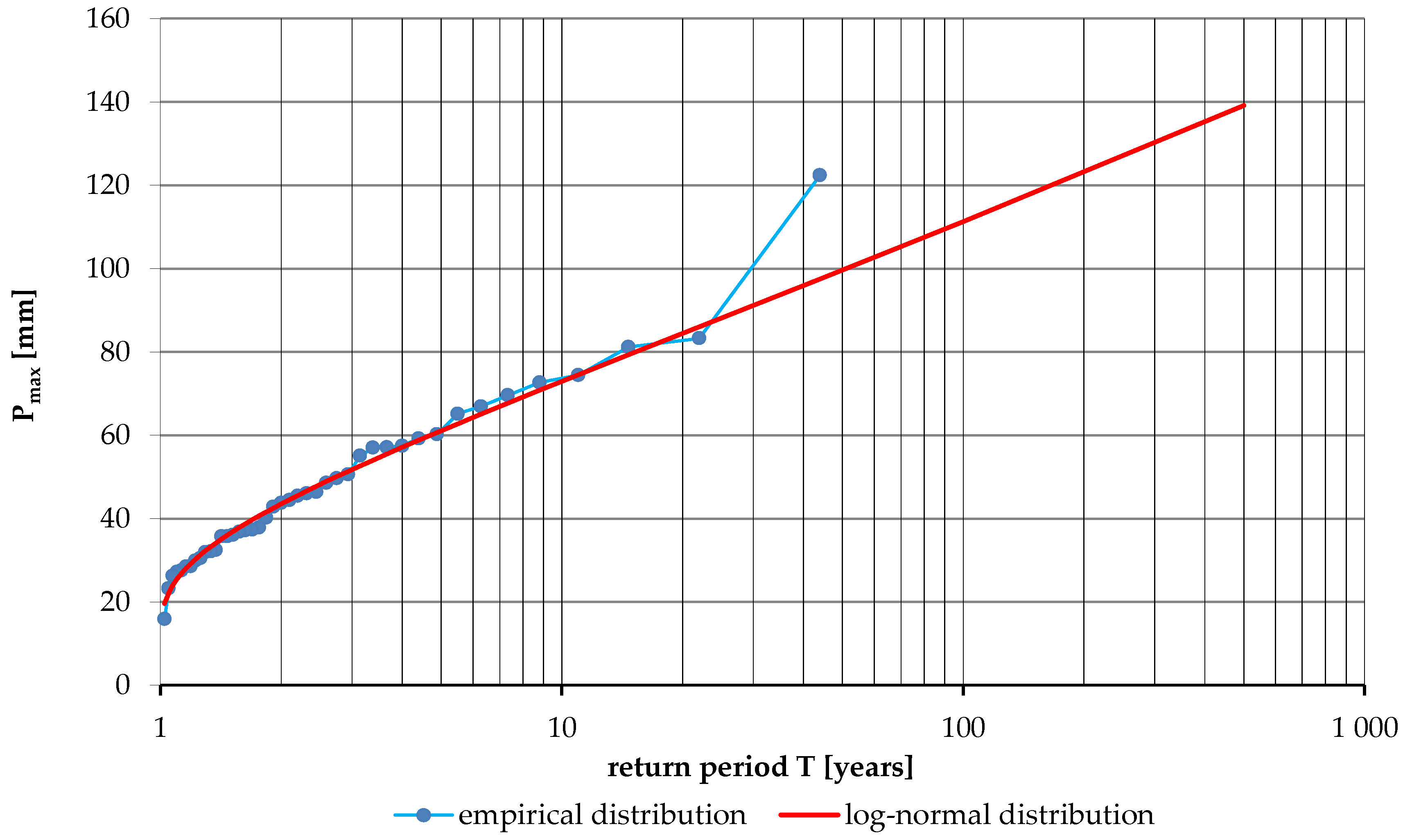
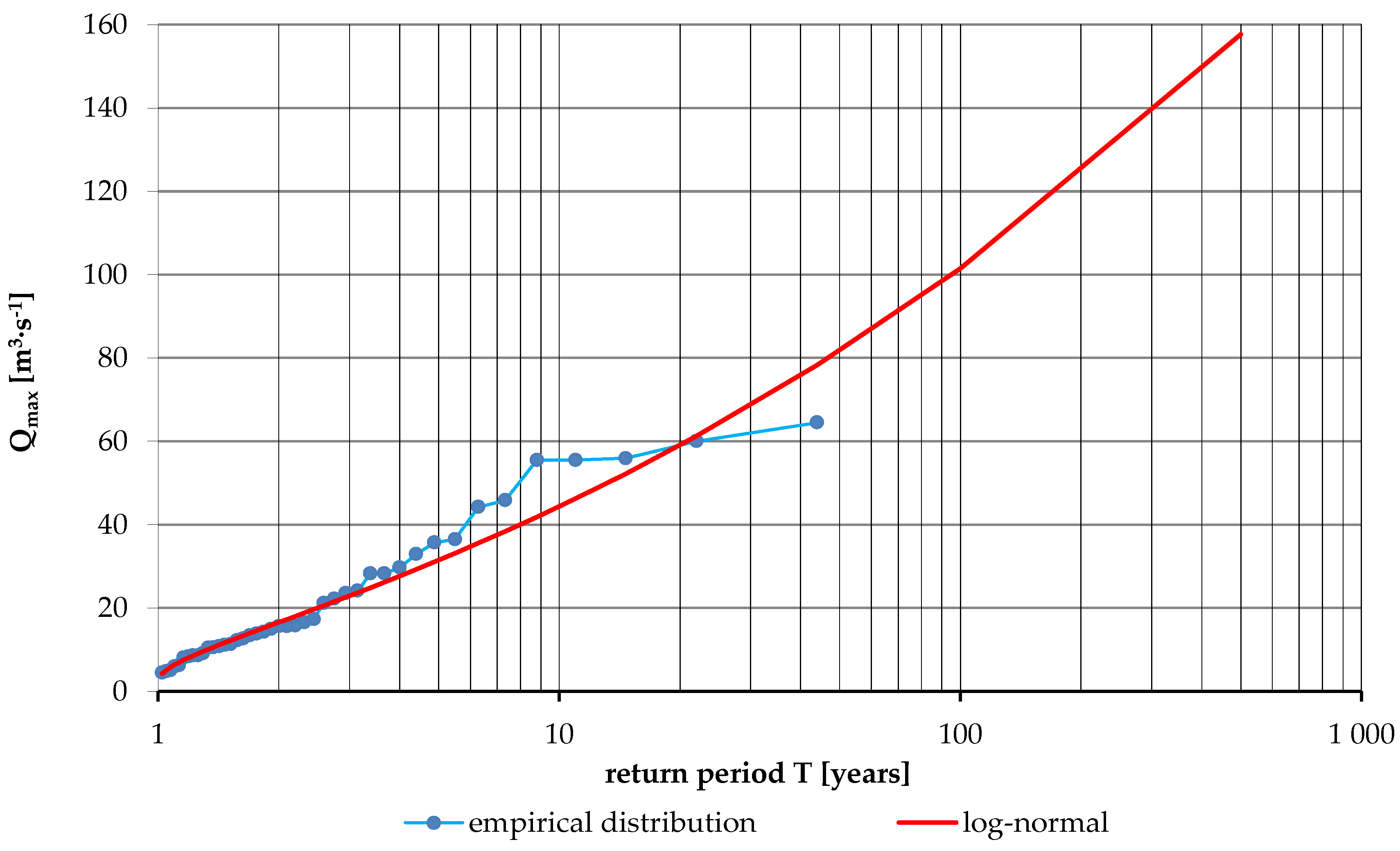
2.3. Calculation of Maximum Annual Rainfall and Flows with Specific Occurrence Frequency

In this study, it was assumed that the maximum flow with a specific frequency (Q_T) is caused by the occurrence of rainfall with the same frequency [22]. The Q_T flows were determined in order to assess the quality of the hydrological rainfall-runoff models. The tests were performed for the frequencies related to the return periods of 500, 100, and 10 years. The calculations were performed applying the log-normal distribution, which is described as [23]:

$$f\left(x\right)=\frac{1}{(x-\epsilon )\alpha \sqrt{2\pi }}exp\left[-\frac{1}{2}{\left(\frac{ln(x-\epsilon )-\mu }{\alpha }\right)}^2\right]$$

(7)

$$x_p=\exp \left[\mu +\frac{\alpha \sqrt{2}}{\mathrm{erf}\left(2\right(1-p)-1)}\right]+\epsilon$$

(8)

where:

• x_p—quantile of the theoretical log-normal distribution;
• ε—lower string limit;
• erf(2(1 − p) − 1)—Gauss error function.

After determining the representative rainfall, the concentration time for the catchment was determined using the Giandotti formula [24]. Rainfall was then determined for a duration equal to the concentration time, using Lambor reduction curves. Then the pattern of the design hyetograph was determined with the DVWK method [25].

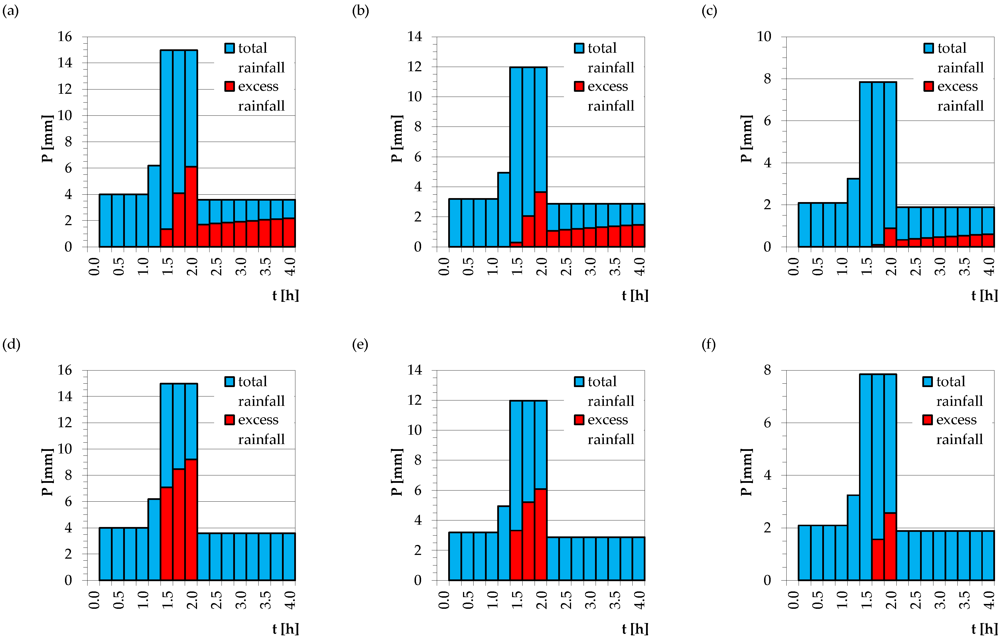
2.4. Determination of the Design Hydrograph

The design hydrograph was determined with the models: Snyder, SCS-UH, and EBA4SUB. In the Snyder and SCS-UH models, the excess rainfall was determined using the SCS-CN method, while in EBA4SUB the CN4GA procedure was used. In order to characterize the design hydrograph shape, the values of wave slenderness coefficients were determined from the relationship [26]:

$$\alpha = \frac{t_o}{t_s}$$

(9)

where:

• t_o—wave fall time (h);
• t_s—wave rise time (h);

The SCS-CN method is a common method used for estimating the direct runoff in the world. It was developed in USA, mostly for assessing the runoff in small agricultural catchments [27,28]. In the SCS-CN method, the excess rainfall depends on the category of soils, on the land use, and on the soil moisture before the considered rainfall occurs. All these factors were considered in the CN parameter (Curve Number) which is an empirical parameter used in hydrology for predicting direct runoff or infiltration from total rainfall. The ranges of CN is from 0 to 100. The amount of excess rainfall was calculated from the relationship [29,30,31]:

$$Pe=\{\begin{array}{c}\frac{{(P - 0.2S)}^2}{P + 0.8S}, \mathrm{when} P \ge 0.2S\\ 0, \mathrm{when} P < 0.2S\end{array}$$

(10)

where:

• P_e—excess rainfall (mm);
• P—total rainfall (mm);
• S—maximum potential catchment retention (mm).

The maximum potential retention of the catchment is directly related to the CN parameter and is described by the equation:

$$S=25.4·(\frac{1000}{CN}-10)$$

(11)

The CN parameter was determined for the second moisture level (AMC II), calculating it for the catchment as a weighted average, according to the guidelines presented in [32].

To determine the design hydrograph with the Snyder model, it is necessary to know the peak flow, delay time, and the time to reach the peak. These parameters are estimated from the relationship [33,34,35]:

T_L = C_t·(L·L_c)^0.3

(12)

where:

• T_L—delay time (h);
• C_t—factor related to catchment retention (-);
• L—maximum distance along the watercourse from the outlet cross-section to the drainage divide (km);
• L_c—distance along the main watercourse from the outlet cross-section to the centroid of the catchment (km).

$$Q_p = \frac{2.78·C_p·A}{T_L}$$

(13)

where:

• Q_p—peak flow of the unit hydrograph (m³·s⁻¹·mm);
• C_p—empirical coefficient resulting from the simplification of the hydrograph to triangular shape (-);
• A—catchment area (km²).

The SCS-UH model belongs to the group of unit hydrograph methods. The unit hydrograph is simplified to form a triangle, and it is caused by an excess unitary rainfall uniformly distributed throughout the entire catchment area. The size of the peak flow is expressed by the formula [36]:

$$q_p = \frac{c·A}{T_p}$$

(14)

where:

• q_p—peak flow of the unit hydrograph (m³·s⁻¹·mm);
• c—conversion factor (c = 0.208) (-);
• T_p—flood rise time, (h), calculated as:

  $$T_P=\frac{D}{2}+T_{LAG}$$

  (15)

where:

• D—duration of excess rainfall (h);
• T_LAG—lag time in the SCS-UH method, (h), calculated as:

  $$T_{LAG}=\frac{{(3.28·L·1000)}^{0.8}·{(\frac{1000}{CN}-9)}^{0.7}}{1900·\sqrt{I}}$$

  (16)

where:

• L—maximum length of the runoff path (km);
• CN—Curve Number value (-);
• I—average catchment slope (%).

The main element determining the shape of the design hydrograph determined with the NRCS-UH method is the Peak Rate Factor (PRF). The value recommended by NRCS is 484. In the case of small mountain catchments characterized by a fast response to rainfall, the value of this indicator should be higher. In this work, analyses using the SCS-UH model were carried out for PRF values equal to 484 and 600.

In order to use the EBA4SUB model to determine the runoff hydrograph, it was necessary to use the DEM of the catchment and to determine the value of the CN parameter (the same of other methodologies). The excess rainfall was subsequently determined based on the CN4GA procedure [37]. This method is based on two stages. In the first, the excess rainfall is determined based on the NRCS-CN method (Equation (10)). In the second stage, the temporal distribution of the excess rainfall inside the event is determined using the Green–Ampt equation:

$$q_0\left(t\right)=\{\begin{array}{c}i\left(t\right), \mathrm{for} t<t_p\\ K_s\left(1+\frac{\mathsf{\Delta }\theta \mathsf{\Delta }H}{I\left(t\right)}\right), \mathrm{for} t>t_p\end{array}$$

(17)

where:

• q₀—infiltration indicator;
• t_p—ponding time;
• K_s—saturated hydraulic conductivity;
• I—cumulative infiltration;
• Δθ—change in soil-water content between the initial value and the field saturated soil-water content;
• ΔH—difference between the pressure head at the soil surface and the matric pressure head at the moving wetting front.

The solution of Equation (17) requires the calibration of the K_s parameter. At the beginning, the value of this parameter is assumed based on the case study soil group. Then the cumulative infiltration is calculated, and its value is compared to that obtained from the NRCS-CN method. The value of the K_s parameter changes until the cumulative infiltration from Equation (17) is equal to that calculated using the NRCS-CN method. After determining the amount of excess rainfall, the instantaneous unit hydrograph is determined based on the width function described by the relationship [38]:

$$WFIUH\left(t\right)=\frac{L_c\left(x\right)}{V_c\left(x\right)}+\frac{L_h\left(x\right)}{V_h\left(x\right)}$$

(18)

where:

• L_c, L_h—hillslope and channel flow paths, functions of DEM cell x, respectively;
• V_c, V_h—runoff velocity for hillslope cells and flow channel cells.

After defining WFIUH, the final design hydrograph Q(t) is determined, described by the following relationship:

$$Q\left(t\right)=A{{\displaystyle \int }}_0^{t}WFIUH(t - \tau )P_n(\tau )d\tau$$

(19)

where:

• A—catchment area (km²);
• T—duration of rainfall (h);
• P_n(t)—excess rainfall determined by the CN4GA method (mm/h).

2.5. Assessment of Quality of Analysed Hydrological Models

The quality of the simulations obtained using the Snyder, NRCS-UH and EBA4SUB models was assessed using the Mean Absolute Percentage Error (MAPE), which is described by the following relationship [39]:

$$MAPE=\frac{Q_{s,max}-Q_{m,max}}{Q_{s,max}}·100 [\%]$$

(20)

where:

• Q_m,max—maximum flow with a certain frequency of occurrence, calculated using rainfall-runoff models (m³·s⁻¹);
• Q_s,max—maximum flow with a specified frequency of occurrence, calculated using the log-normal distribution on observed data (m³·s⁻¹).

3. Results

3.1. Hydrometeorological Data Verification

The results of the analysis related to the hydrometeorological data verification are presented in

Table 1. The results of the significance analysis of the trend for the observation series P_max and Q_max in the Grajcarek catchment.

Characteristic	Zc	pc	Varc	n/n *	Z	p	Var
Pmax	1.582	0.114	7721.554	0.846	1.455	0.146	9129.333
Qmax	1.143	0.253	9766.667	1.000	1.143	0.253	9766.667

Z_c—modified value of normalized MK statistics; p_c—modified value of test probability, Var_c—modified value of variance, n/n *—effective number of observations, Z—value of normalized statistics MK, p—test probability, Var—variance.

.

Based on the results summarized in Table 1, it was found that for the analyzed multi-year period, there were no statistically significant trends in the series of observations of the maximum annual daily rainfall and flow. This is evidenced by the values of the Z_c Mann-Kendall statistics, which assume smaller quantities than the critical value, for the significance level α = 0.05 at 1.96. In the case of the results for the P_max observation series, the effective number of observations (n/n *) takes values other than 0, which indicates autocorrelation between individual variables. However, it does not affect the conclusions made using the analyzed test. Similar results for rainfall in southern Poland were obtained by Niedźwiedz et al. [40] and Młyński et al. [41]. These studies showed that the rainfall in this region is characterized by growing but not statistically significant trends, and all changes in the amount of rainfall are caused by irregular fluctuations. Slight trends in changes in the amount of rainfall are reflected in the flood flows in the upper Vistula catchment. Research conducted by Kundzewicz et al. [42], Wałęga et al. [43] and Młyński et al. [44] have shown a steady state of flood flows in southern Poland over the last several years. Due to their geological structure, morphometric characteristics, and land use, mountainous basins of the upper Vistula river catchment are sensitive to the occurrence of intense rainfall. Hence, the rhythm of their course is repeated by the rhythm of rainfall [45]. Therefore, it can be pointed out that there is a relationship between the maximum annual daily rainfall and the maximum flow.

3.2. Determination of Rainfall and Peak Flows at a Specific Occurrence Frequency

Rainfall and maximum flow of a certain frequency were determined using the log-normal distribution. The results of the calculations are presented in Figure 2 and Figure 3. Based on the analyses, the following rainfall values have been determined for return periods of 500, 100, and 10 years: 139; 111; and 73 mm respectively. The following values were obtained for peak flows: 157.660; 101.469; and 44.470 m³∙s⁻¹ for return periods of 500, 100, and 10 years, respectively. The use of log-normal distribution in the analysis for calculating the maximum daily annual rainfall with a specific frequency of occurrence was supported by research conducted by Młyński et al. [46] It has been shown that this function is best suited to the empirical rainfall distribution P_max, hence it can be the basis for determining the course of design rainfall. In the work Młyński et al. [47] it has been shown also that the same function describes at best the empirical distributions of Q_max flows in the upper Vistula catchment. The log-normal distribution belongs to the family of right-handed heavy-tail functions, hence it is widely used to describe extreme hydrometeorological phenomena, as supported by Kuczera [48] and Strupczewski et al. [49]

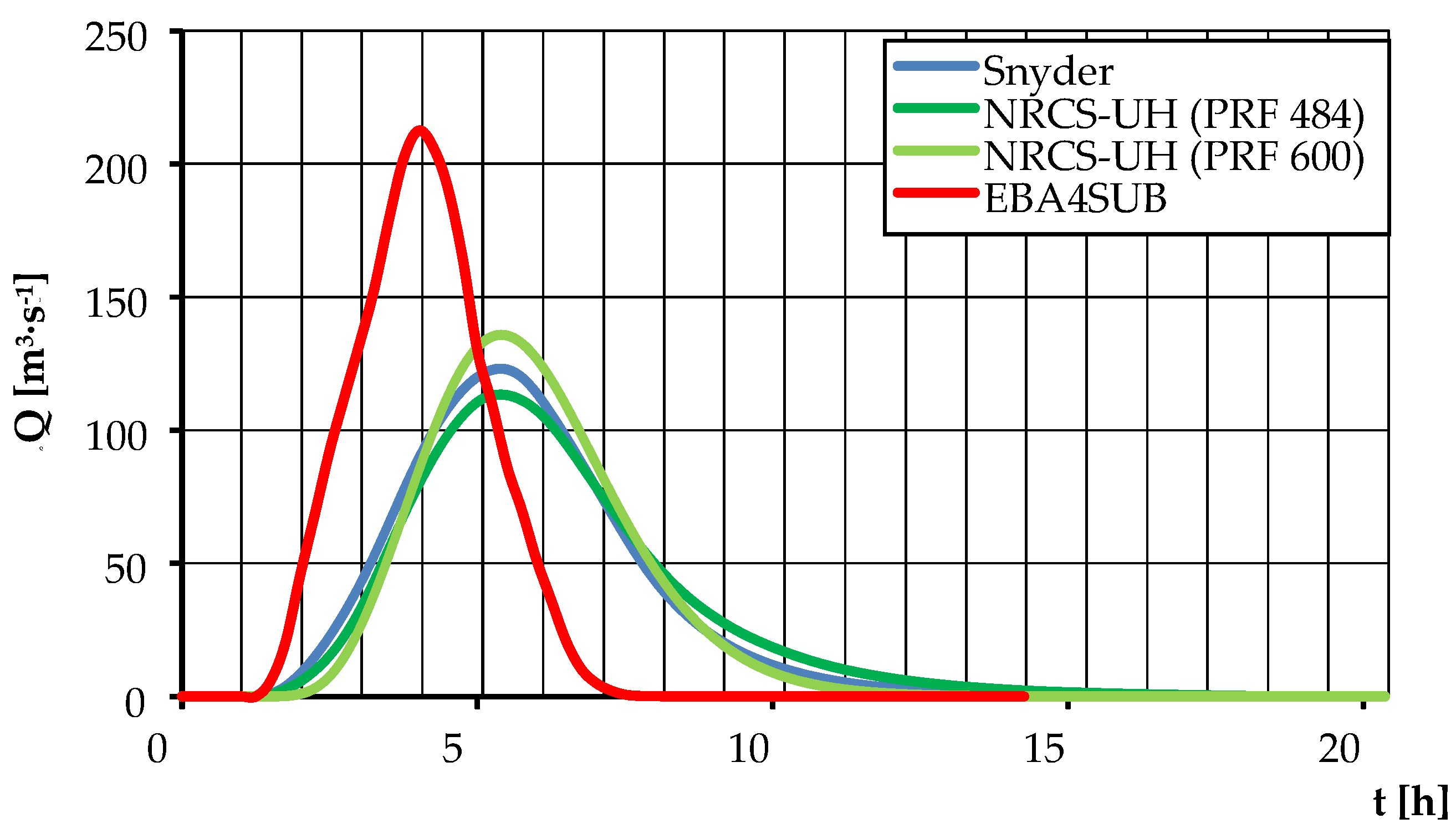
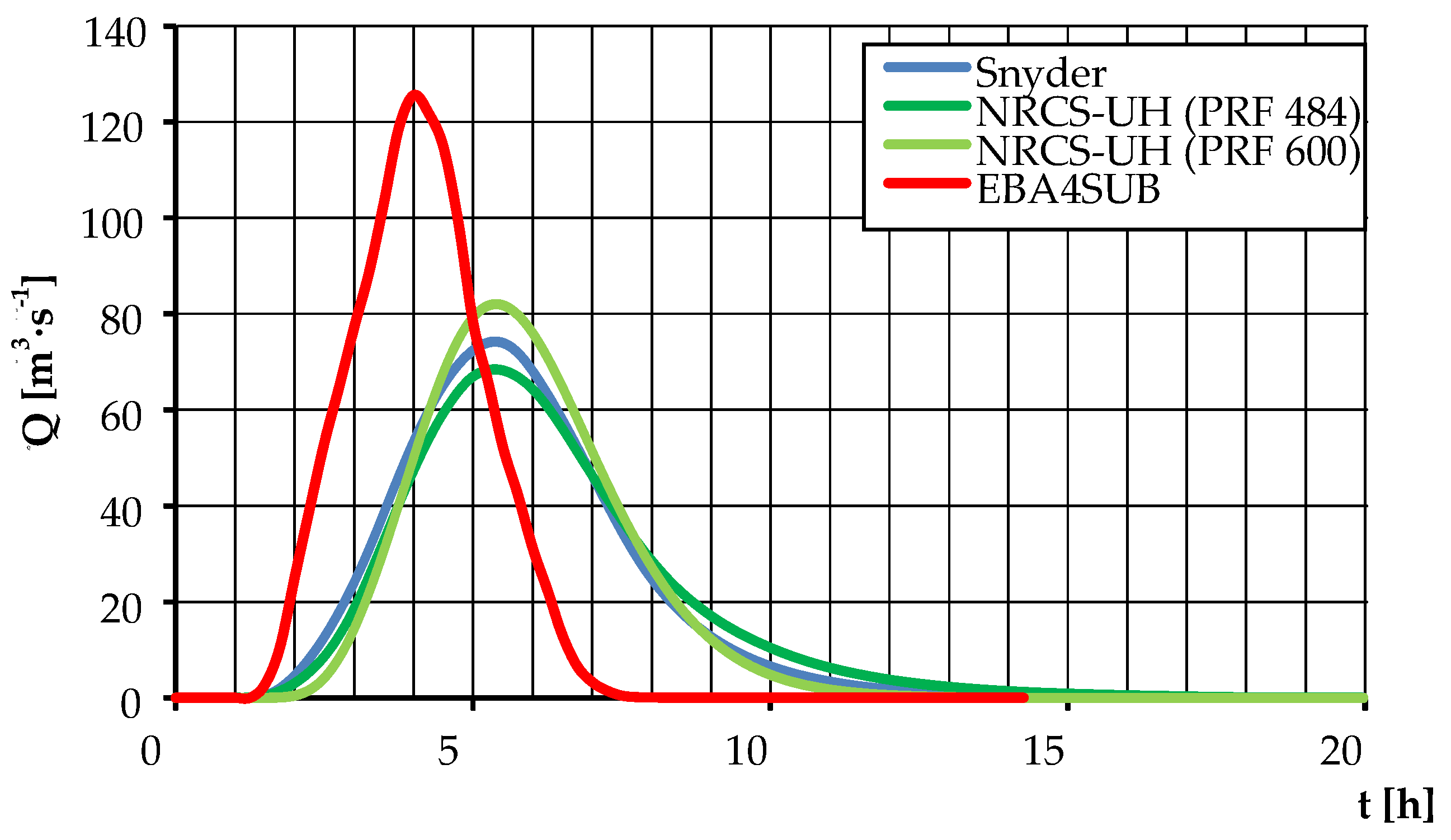
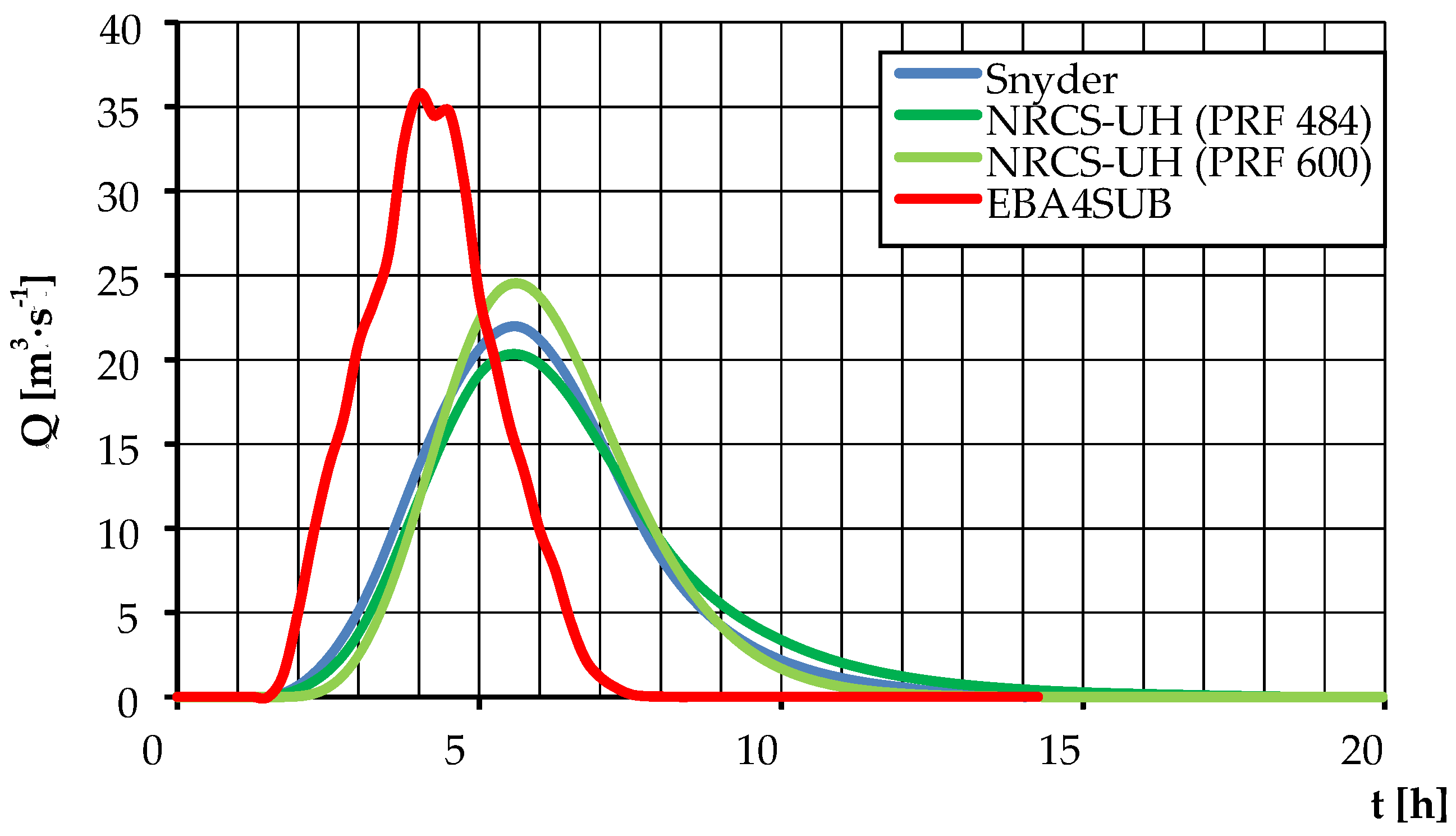
3.3. Determination of Design Hydrographs Employing the Selected Rainfall-Runoff Models

In order to be able to use the selected rainfall-runoff models, the excess rainfall heights were determined using the NRCS-CN and CN4GA methods. The results of the calculations are summarized in

Table 2. Excess rainfall amounts determined by the NRCS-CN and CN4GA methods.

Return Period	Tc (h)	CN	P (mm)	Pnet (mm)
500	4	68.1	95.8	24.7
100			76.6	14.6
10			50.2	4.1

. Figure 4 shows the excess rainfall hyetographs against the background of total rainfall.

The amount of total rainfall P for the assumed return periods was determined by reducing the amounts calculated using the log-normal distribution to an amount corresponding to a duration of 4 h, due to the calculated concentration time. AMC II was assumed for the calculation of the CN parameter. It should be emphasized, however, that assuming this level for ungauged mountainous catchments is a significant problem because the initial soil moisture conditions are determined not only by atmospheric rainfall but also by the high level of the groundwater table and the occurrence of poorly permeable soils that hinder infiltration. These factors lead to a decrease in the retention capacity of the catchment. This is particularly evident in mountainous areas. Therefore, the adoption of a low level of moisture can lead to an underestimation of the size of the design hydrograph. If the soil moisture level is set too high, the floods can be greatly overestimated. Therefore, it is necessary to verify the assumptions in relation to local environmental conditions to reduce modeling uncertainty [50]. Moreover, it should be emphasized that using the CN values proceeded by the standardized procedure, the SCS-CN method can overestimate runoffs for high rainfall events, whereas it underestimates runoffs for low depth rainfall events [51].

The shape of design hydrograph for given return periods was determined using the Snyder, NRCS-UH, and EBA4SUB models. In the case of the first two models, the analysis was carried out for excess rainfall calculated by the NRCS-UH method. For the EBA4SUB model, the excess rainfall determined by the CN4GA method was used.

Table 3. Characteristics of design hydrographs determined using the analyzed models.

Characteristic	Snyder			NRCS-UH			EBA4SUB
	500	100	10	500	100	10	500	100	10
Qmax [m3·s−1]	122.909	74.191	21.975	113.235 *	68.424 *	20.329 *	212.531	125.602	35.779
				135.483 **	82.059 **	24.529 **
V [mln m3]	2.291	1.377	0.403	2.291	1.377	0.403	2.078	1.226	0.346
t [h]	15.250	15.250	15.000	21.750 *	21.750 *	21.500 *	6.800	6.800	6.500
				16.000 **	15.750 **	15.500 **
α [–]	2.100	1.952	1.905	3.150 *	3.000 *	2.950 *	1.545	1.545	1.500
				2.095 **	2.095 **	2.150 **

* PRF (peak rate factor) = 484, ** PRF = 600.

summarizes the characteristics of design hydrographs. Figure 5, Figure 6 and Figure 7 present their shapes for the investigated return periods.

Based on the results summarized in Table 3 and Figure 5, Figure 6 and Figure 7, it was found that the highest values of peak flows were obtained using the EBA4SUB model. This is due to the fact that the EBA4SUB model takes into account the surface runoff speed when calculating the width function from the formula (18). The analysed catchment has a mountainous character, so the runoff speeds will be higher due to the greater slopes. Therefore, the catchment response for the EBA4SUB model will be faster than for the others. In the NRCS-UH model, the catchment topography is considered indirectly by the PRF value, however, in this case, a generalization is assumed that the same PRF value is valid for the entire catchment, which is typical for a lumped model. In the case of the EBA4SUB model, the surface flow velocity is calculated for each pixel of the DEM, and is dependent on the specific pixel slope, so it characterizes the dynamics of runoff for the entire catchment. For the Snyder model, the topography of the terrain is included in the Ct parameter. However, the model is not very sensitive to changes in this parameter [26]. Regarding the peak flow values for Snyder and NRCS-UH, they are comparable. It should be emphasized that higher values in the peak flow for the NRCS-UH model were obtained assuming the PRF value as 600. Due to their geological structure and physiographic characteristics, small mountainous catchments are characterized by a rapid response to the occurring rainfall. As a result, the peak flow is violent and the flood duration is relatively short. Higher PRF values reflect the shape of such floods. Conversely, lower values should be assumed for lowland and plain catchments [52]. The average peak flows obtained with the Snyder and NRCS-UH models are 40% smaller compared to the corresponding peak flows determined by the EBA4SUB model, for each return period. Despite significant differences in flows between EBA4SUB, Snyder and NRCS-UH, the volume of flood is similar and amounts to slightly over 2 million m³, 1 million m³ and ca. 0.4 million m³ for return periods of 500, 100, and 10 years, respectively. Similar volumes result from the fact that the basic information on excess rainfall in the CN4GA model are values determined using NRCS-CN. The CN4GA method first calculates the cumulative excess rainfall using the NRCS-CN method. The CN4GA model is then used to determine the distribution of the excess rainfall over time by taking into account the variable infiltration capacity during soil in the catchment. The shorter peak flow time is the result of the distribution of excess rainfall over time, determined by the CN4GA method (Figure 5). The duration of this fallout is 0.75 h (500 and 100 years return period) and 0.5 h (10 years return period) where for the NRCS-CN method it is 2.8 h and 2.5 h, respectively. Therefore, the effective rainfall intensity for CN4GA is concentrated over a shorter period of time, which is reflected by the shape of the design hydrograph. The slenderness factor, whose values in each case are greater than 1.0, indicates that the water level increased rapidly until the peak and then it fell slowly. Hence, it can be concluded that there is an imbalance between volumes for the rising and falling parts, where the falling volume was in each case larger. Due to its simplicity, the EBA4SUB model can be alternatively used to determine the shape of design hydrographs in uncontrolled catchments. Its use consists basically of three stages: determining the distribution of the design rainfall, determining the excess rainfall, and determining the design hydrograph from the catchment. The simplicity of application of the model in hydrological analyses means that it can be successfully used by practitioners to determine flood hazard zones or to determine the size of reliable flows for the design of hydrotechnical constructions. All analysed models have some limitations. They are sensitive to changes in the CN parameter, which determines the amount of excess rainfall, which translates into the values of the peak flow. Research carried out by Maidment and Hoogerwerf [53] showed that an increase in the CN parameter by 1% increases the peak flow determined from the model also by approximately 1%. In the case of the Snyder model, the coefficient values depending on the retention capacity of the catchment must be estimated for its identification. Currently, there are no specific guidelines indicating which values of these parameters should be assumed in relation to particular characteristics of the catchment, which is why designers do it in a subjective way. The first attempts to make the parameters of the Snyder model dependent on the catchment characteristics in Polish conditions were carried out by Wałęga [54], but the obtained results require verification in the Carpathian catchments. Changes in the values of individual parameters may, as a consequence, affect the sizes of floodplains or planned water management facilities. The conducted research allowed to state that the EBA4SUB model does not have such limitations. Model parameters are determined directly on the basis of physiographic characteristics of the catchment, which precludes the subjectivity of their determination.

However, it should be emphasized that further research should be carried out regarding the possibility of the use of EBA4SUB in uncontrolled mountainous catchments. Such studies should primarily focus on determining the reference shape of the design hyetograph. A research conducted by Młyński et al. [44] concluded, for instance, that even small changes in the design hyetograph shape can cause differences in peak flows, calculated using the model, of more than 10%.

The Grajcarek drainage catchment is strongly asymmetrical, i.e., most of its tributaries are right-bank inflows and are what causes that the shape of the catchment to be close to the oval. Hence the concentration time is relatively short and it can contribute to a relatively fast rise of hydrographs. It is defined very well by the EBA4SUB model compared to classic models, which take less account of catchment asymmetry in the hydrographs shape.

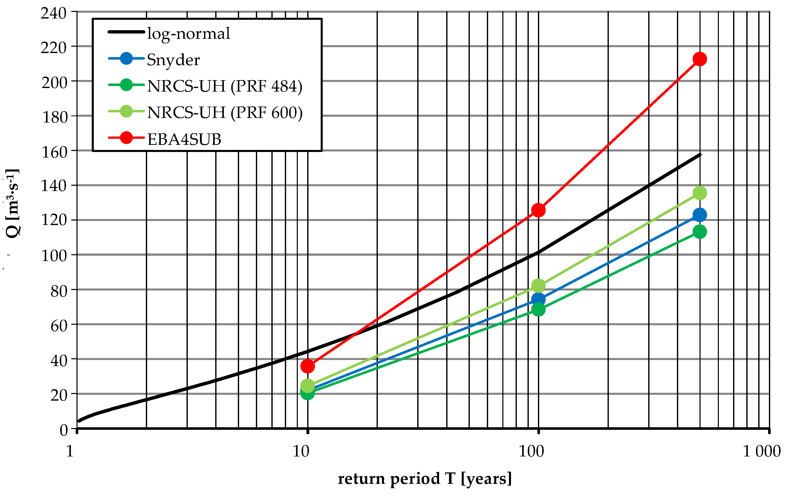
3.4. Evaluation of the Quality of Analysed Hydrological Models

The results of the calculations regarding the quality of hydrological models using the MAPE indicator are presented in

Table 4. Mean Absolute Percentage Error (MAPE) index values for the hydrological models analyzed.

Model	MAPE [%]
	500	100	10
Snyder	22.0	26.9	50.5
NRCS-UH (PRF 484)	28.2	32.6	54.2
NRCS-UH (PRF 600)	14.1	19.1	44.7
EBA4SUB	−34.8	−23.8	19.4

. Figure 8 presents the values of peak flows for the analysed return periods obtained using the analysed rainfall-runoff models against the background of the probability distribution curve determined by the log-normal distribution.

Based on the results shown in Figure 8, it was found that Q_T values determined using the Snyder and NRCS-UH models are lower, as respect to the corresponding values determined using the log-normal distribution. For the EBA4SUB model, the calculated Q₅₀₀ and Q₁₀₀ are higher than the statistical method. Based on the values listed in Table 4, it was found that for Q₅₀₀, the NRCS-UH (PRF 600) model was characterized by the smallest relative error. It should be emphasized, however, that the average value of this error, for all return periods, is lower for the EBA4SUB and NRCS-UH (PRF 600) models and amounted to 26% for both. For Snyder it was 33%, while for NRCS-UH (PRF 484) it was 38%. The calculations carried out confirm that the EBA4SUB model can be an alternative to the Snyder and NRCS-UH models. In the case of lower return periods, the EBA4SUB model gives peak flows more similar to the observed ones. This provides some security for uncontrolled catchments, where there is no hydrometric information. This could reduce the risk of designating too-narrow flood hazard zones or undersizing hydrotechnical constructions in the light of weather phenomena, the course of which is becoming increasingly extreme.

The main aim of EBA4SUB is to provide an accurate estimation of the design hydrograph, minimizing at the same time the subjectivity of the practitioner related to the choice of the input parameters. Practically, the EBA4SUB model reduces the uncertainty in the modeling of both the infiltration process (thanks to the automatic estimation of CN) and both the propagation process (thanks to the automatic estimation of concentration time). In doing so, EBA4SUB proposes a framework that, on the same watershed and with the same input data, provides similar results when it is applied by two different analysts in two different moments. This is crucial because when using different approaches, as respect to EBA4SUB, like the well-known rational formula, it recognized a great uncertainty in the estimation of the runoff coefficient or the concentration time. Moreover, from a methodological point of view, EBA4SUB is characterized by the following advantages. First, in excess rainfall estimation, thanks to the CN4GA structure and its automatic calibration, it benefits from the accuracy of a physically based infiltration scheme (the Green–Ampt equation) mixed with the simplicity of an empirical approach (the CN method). Second, for excess rainfall-direct runoff transformation, it determines the IUH (instantaneous unit hydrograph) shape using detailed geomorphological information pixel by pixel, avoiding the use of synthetic methods.

The proposed procedure can help in assessing the influence of land abandonment on a watershed scale on the surface runoff, since it allows an immediate estimation of design hydrograph based on a hypothesis of changes of CN and concentration time that could be due to land use or land cover modifications. Indeed modifications in land use or land cover are reflected by changes in CN, affecting the infiltration process, and by changes in concentration time, altering surface flow velocities that at a cascade affect the excess rainfall-direct runoff transformation [55]. Regarding agricultural practices, it is well known in the literature that the impact of agriculture leads to a reduction in vegetation cover and to an increase of both soil erosion rates and flood formation phenomena. As an example, Cerdà et al. [56] found that when a field is abandoned, a sudden increase in surface runoff (more than two times) can be expected before vegetation recovers, so there is a particular need to apply nature-based soil and water conservation strategies to prevent soil erosion. Conversely, regarding forestry practices, Keesstra [57] found that the basin extensive reforestation of the Dragonja catchment, which occurred in Slovenia from 1945 to 2008, reduced the discharge of the river across the entire spectrum of the flow, in particular for high return period events. Finally, regarding urbanization processes, Recanatesi et al. [58] found that uncontrolled land degradation can severely increase flood risk, and that best management practices are strongly needed, since they can help in mitigating the flood risk by up to 90%.

4. Conclusions

The purpose of the research was to analyze the possibility of using the EBA4SUB model to determine design hydrographs in mountainous catchments. Considering the obtained results, it was found that this model can be an alternative to commonly used rainfall-runoff models such as Snyder and NRCS-UH. The EBA4SUB model provides values for peak flows, with a specific frequency of occurrence, relatively similar in respect to values obtained by the statistical method. Therefore, it can be recommended as one of the alternatives to determine the shape of design hydrographs in uncontrolled and mountainous basins. It should be emphasized, however, that the decisive factor influencing the performances of hydrological rainfall-runoff models is the quality of meteorological data constituting the input signal. Therefore, it is recommended to use the model in catchments where this information has been fully verified.

Considering the topographic characteristics of the catchments that affect the asymmetry of its river network, like height differences, runoff length and therefore the time of wave transition, the EBA4SUB model appears to show less subjectivity in runoff calculation processes. Practical verification will be possible by using the model to delineate flood risk zones and compare them with the corresponding results obtained with other methods or with observed ones.

References

1. Cerdà Bolinches, A.; Lucas Borja, M.E.; Úbeda, X.; Martínez Murillo, J.F.; Keesstra, S. Pinus halepensis M. versus Quercus ilex subsp. Rotundifolia L. runoff and soil erosion at pedon scale under natural rainfall in Eastern Spain three decades after a forest fire. For. Ecol. Manag. 2018, 400, 447–456. [Google Scholar] [CrossRef] [Green Version]
2. Van Eck, C.M.; Nunes, J.P.; Vieira, D.C.; Keesstra, S.; Keizer, J.J. Physically-Based modelling of the post-fire runoff response of a forest catchment in central Portugal: Using field versus remote sensing based estimates of vegetation recovery. Land Degrad. Dev. 2016, 27, 1535–1544. [Google Scholar] [CrossRef]
3. Banach, W. Determination of synthetic flood hydrograph in ungauged catchments. Infrastruct. Ecol. Rural Areas 2011, 12, 147–156. [Google Scholar]
4. Salami, A.W.; Bilewu, S.O.; Ibitoye, A.B.; Ayanshola, A.M. Runoff hydrographs using Snyder and SCS unit hydrograph methods: A case study of selected rivers in south west Nigeria. J. Ecol. Eng. 2017, 18, 25–34. [Google Scholar] [CrossRef] [Green Version]
5. Gądek, W. Assessment of limingraph data usefulness for determining the hypothetical flood waves with the Cracow method. J. Water Land Dev. 2014, 21, 71–78. [Google Scholar] [CrossRef] [Green Version]
6. Gądek, W.; Środula, A. The evaluation of the design flood hydrographs determined with the Hydroproject method in the gauged catchments. Infrastruct. Ecol. Rural Areas 2014, 4, 29–47. [Google Scholar]
7. Pietrusiewicz, I.; Cupak, A.; Wałęga, A.; Michalec, B. The use of NRCS synthetic unit hydrograph and Wackerman conceptual model in the simulation of a flood wave in uncontrolled catchment. J. Water Land Dev. 2014, 23, 53–59. [Google Scholar] [CrossRef] [Green Version]
8. Wypych, A.; Ustrnul, Z.; Henek, E. Meteorological hazards—Visualization system of national protection against extreme hazards for Poland. Meteorol. Hydrol. Water Manag. 2014, 2, 37–42. [Google Scholar] [CrossRef]
9. Karabová, B.; Sikorska, A.; Banasik, K.; Kohnová, S. Parameters determination of a conceptual rainfall-runoff model for a small catchment in Carpathians. Ann. Wars. Univ. Life Sci. SGGW 2012, 44, 155–162. [Google Scholar]
10. Wałęga, A.; Młyński, D. Seasonality of median monthly discharge in selected Carpathian rivers of the upper Vistula basin. Carpath. J. Earth Environ. Sci. 2017, 12, 617–628. [Google Scholar]
11. Tolentino, P.L.M.; Poortinga, A.; Kanamaru, H.; Keesstra, S.; Maroulis, J.; David, C.P.C.; Ritsema, C.J. Projected impact of climate change on hydrological regimes in the Philippines. PLoS ONE 2016, 11, e0163941. [Google Scholar] [CrossRef] [Green Version]
12. Xu, J.; Wang, S.; Bai, X.; Shu, D.; Tian, Y. Runoff response to climate change and human activities in a typical karst watershed, SW China. PLoS ONE 2018, 13, e0193073. [Google Scholar] [CrossRef] [PubMed]
13. Blair, A.; Sanger, D.; White, D.; Holland, A.F.; Vandiver, L.; Bowker, C.; White, S. Quantifying and simulating stormwater runoff in watersheds. Hydrol. Process. 2012, 28, 559–569. [Google Scholar] [CrossRef]
14. Banasik, K.; Rutkowska, A.; Kohnová, S. Retention and Curve Number variability in a small agricultural catchment: The probabilistic approach. Water 2014, 6, 1118–1133. [Google Scholar] [CrossRef]
15. Kowalik, T.; Wałęga, A. Estimation of CN Parameter for small agricultural watersheds using asymptotic functions. Water 2015, 7, 939–955. [Google Scholar] [CrossRef] [Green Version]
16. Wałega, A.; Książek, L. Influence of rainfall data on the uncertainty of flood simulation. Soil Water Res. 2016, 11, 277–284. [Google Scholar] [CrossRef] [Green Version]
17. Grimaldi, S.; Petroselli, A. Do we still need the Rational Formula? An alternative empirical procedure for peak discharge estimation in small and ungauged basins. Hydrol. Sci. J. 2015, 60, 67–77. [Google Scholar] [CrossRef]
18. Piscopia, R.; Petroselli, A.; Grimaldi, S. A software package for the prediction of design flood hydrograph in small and ungauged basins. J. Agric. Eng. 2015, 432, 74–84. [Google Scholar]
19. Petroselli, A.; Grimaldi, S. Design hydrograph estimation in small and fully ungauged basin: A preliminary assessment of the EBA4SUB framework. J. Flood Risk Manag. 2018, 11, 197–2010. [Google Scholar] [CrossRef]
20. Sun, S.; Barraud, S.; Branger, F.; Braud, I.; Castebrunet, H. Urban hydrology trend analysis based on rainfall and runoff data analysis and conceptual model calibration. Hydrol. Process. 2017, 31, 1349–1359. [Google Scholar] [CrossRef] [Green Version]
21. Operacz, A.; Wałęga, A.; Cupak, A.; Tomaszewska, B. The comparison of environmental flow assessment—The barrier for investment in Poland or river protection? J. Clean. Prod. 2018, 193, 575–592. [Google Scholar] [CrossRef]
22. Viglione, A.; Blöschl, G. On the role of storm duration in the mapping of rainfall to flood return period. Hydrol. Earth Syst. Sci. Discuss. 2008, 5, 3419–3447. [Google Scholar] [CrossRef]
23. Hogg, R.V.; Craig, A.T. Introduction to Mathematical Statistics; Macmilan Publishing Co.: New York, NY, USA, 1978. [Google Scholar]
24. Grimaldi, S.; Petroselli, A.; Tauro, F.; Porfiri, M. Time of concentration: A paradox in modern hydrology. Hydrol. Sci. J. 2012, 57, 217–228. [Google Scholar] [CrossRef] [Green Version]
25. Wałęga, A.; Drożdżal, E.; Piórecki, M.; Radoń, R. Some problems of hydrology modelling of outflow from ungauged catchments with aspect of flood maps design. Acta Sci. Pol. Form. Circumiectus 2012, 11, 57–68. (In Polish) [Google Scholar]
26. Wałęga, A. The importance of calibration parameters on the accuracy of the floods description in the Snyder’s model. J. Water Land Dev. 2016, 28, 19–25. [Google Scholar] [CrossRef]
27. Soulis, K.X.; Dercas, N. Development of a GIS-based Spatially Distributed Continuous Hydrological Model and its First Application. Water Int. 2007, 32, 177–192. [Google Scholar] [CrossRef]
28. Soulis, K.X.; Valiantzas, J.D. Identification of the SCS-CN Parameter Spatial Distribution Using Rainfall-Runoff Data in Heterogeneous Watersheds. Water Res. Man. 2013, 27, 1737–1749. [Google Scholar] [CrossRef]
29. Xiao, B.; Wang, Q.; Fan, J.; Han, F.; Dai, Q. Application of the SCS-CN Model to Runoff Estimation in a Small Watershed with High Spatial Heterogeneity. Pedosphere 2011, 26, 738–749. [Google Scholar] [CrossRef]
30. Soulis, K.X.; Valiantzas, J.D. SCS-CN parameter determination using rainfall-runoff data in heterogeneous watersheds—The two-CN system approach. Hydrol. Earth Syst. Sci. 2012, 16, 1001–1015. [Google Scholar] [CrossRef] [Green Version]
31. Soulis, K.X. Estimation of SCS Curve Number variation following forest fires. Hydrol. Sci. J. 2018, 63, 1332–1346. [Google Scholar] [CrossRef]
32. Wałęga, A.; Salata, T. Influence of land cover data sources on estimation of direct runoff according to SCS-CN and modified SME methods. Catena 2019, 172, 232–242. [Google Scholar] [CrossRef]
33. Singh, P.K.; Mishra, S.K.; Jain, M.K. A review of the synthetic unit hydrograph: From the empirical UH to advanced geomorphological methods. Hydrol. Sci. J. 2014, 59, 239–261. [Google Scholar] [CrossRef]
34. Sudhakar, B.S.; Anupam, K.S.; Akshay, A.J. Snyder unit hydrograph and GIS for estimation of flood for un-gauged catchments in lower Tapi basin, India. Hydrol. Curr. Res. 2015, 6, 1–10. [Google Scholar]
35. Federova, D.; Kovář, P.; Gregar, J.; Jelínková, A.; Novotná, J. The use of Snyder synthetic hydrograph for simulation of overland flow in small ungauged and gauged catchments. Soil Water Res. 2018, 13, 185–192. [Google Scholar]
36. Amatya, D.M.; Cupak, A.; Wałęga, A. Influence of time concentration on variation of runoff from a small urbanized watershed. GLL 2015, 2, 7–19. [Google Scholar]
37. Grimaldi, S.; Petroselli, A.; Romano, N. Curve-Number/Green–Ampt mixed procedure for streamflow predictions in ungauged basins: Parameter sensitivity analysis. Hydrol. Process. 2013, 27, 1265–1275. [Google Scholar] [CrossRef]
38. Grimaldi, S.; Petroselli, A.; Nardi, F.; Alonso, G. Flow time estimation with variable hillslope velocity in ungauged basins. Adv. Water Resour. 2010, 33, 1216–1223. [Google Scholar] [CrossRef]
39. Kim, S.; Kim, H. A new metric of absolute percentage error for intermittent demand forecast. Int. J. Forecast 2016, 32, 669–679. [Google Scholar] [CrossRef]
40. Niedźwiedź, T.; Łupikasza, E.; Pińskwar, I.; Kundzewicz, Z.W.; Stoffel, M.; Małarzewski, Ł. Climatological background of floods at the northern foothills of the Tatra Mountains. Theor. Appl. Climatol. 2014, 119, 273–284. [Google Scholar] [CrossRef] [Green Version]
41. Młyński, D.; Cebulska, M.; Wałęga, A. Trends, variability, and seasonality of Maximum annual daily precipitation in the upper Vistula basin, Poland. Atmosphere 2018, 9, 313. [Google Scholar] [CrossRef] [Green Version]
42. Kundzewicz, Z.W.; Stoffel, M.; Kaczka, R.J.; Wyżga, B.; Niedźwiedź, T.; Pińskwar, I.; Ruiz-Villanueva, V.; Łupikasza, E.; Czajka, B.; Ballesteros-Canovas, J.A. Floods at the Northern Foothills of the Tatra Mountains—A Polish–Swiss Research Project. Acta Geophys. 2014, 62, 620–641. [Google Scholar] [CrossRef]
43. Wałęga, A.; Młyński, D.; Bogdał, A.; Kowalik, T. Analysis of the course and frequency of high water stages in selected catchments of the Upper Vistula basin in the south of Poland. Water 2016, 8, 394. [Google Scholar] [CrossRef]
44. Młyński, D.; Petroselli, A.; Wałęga, A. Flood frequency analysis by an event-based rainfall-runoff model in selected catchments of southern Poland. Soil Water Res. 2018, 13, 170–176. [Google Scholar]
45. Kundzewicz, Z.W.; Pińskwar, I.; Choryński, A.; Wyżga, B. Floods still pose a hazard. Aura 2017, 3, 3–9. (In Polish) [Google Scholar]
46. Młyński, D.; Wałęga, A.; Stachura, T.; Kaczor, G. A new empirical approach to calculating flood frequency in ungauged catchments: A case study of the upper Vistula basin, Poland. Water 2019, 11, 601. [Google Scholar] [CrossRef] [Green Version]
47. Młyński, D.; Wałęga, A.; Petroselli, A.; Tauro, F.; Cebulska, M. Estimating maximum daily precipitation in the upper Vistula basin, Poland. Atmosphere 2019, 10, 43. [Google Scholar] [CrossRef] [Green Version]
48. Kuczera, G. Robust flood frequency models. Water Resour. Res. 1982, 18, 315–324. [Google Scholar] [CrossRef]
49. Strupczewski, W.G.; Singh, V.P.; Mitosek, H.T. Non-stationary approach to at site flood frequency modeling. III. Flood analysis for Polish rivers. J. Hydrol. 2001, 248, 152–167. [Google Scholar] [CrossRef]
50. Wałęga, A.; Rutkowska, A. Usefulness of the modified NRCS-CN method for the assessment of direct runoff in a mountain catchment. Acta Geophys. 2015, 63, 1423–1446. [Google Scholar] [CrossRef] [Green Version]
51. Soulis, K.X.; Valiantzas, J.D.; Dercas, N.; Londra, P.A. Investigation of the direct runoff generation mechanism for the analysis of the SCS-CN method applicability to a partial area experimental watershed. Hydrol. Earth Syst. Sci. 2009, 13, 605–615. [Google Scholar] [CrossRef] [Green Version]
52. Walega, A.; Amatya, D.M.; Caldwell, P.; Marion, D.; Panda, S. Assessment of storm direct runoff and peak flow rates using improved SCS-CN models for selected forested watersheds in the Southeastern United States. J. Hydrol. Reg. Stud. 2020, 27, 1–18. [Google Scholar] [CrossRef]
53. Maidment, D.W.; Hoogerwerf, T.N. Parameter Sensitivity in Hydrologic Modeling. Technical Report; The University of Texas: Austin, TX, USA, 2002. [Google Scholar]
54. Wałęga, A. An attempt to establish regional dependecies for the parameter calculation of the Snyder’s syntetic unit hydrograph. Infrastruct. Ecol. Rural Areas 2012, 2, 5–16. [Google Scholar]
55. Ignacio, J.A.F.; Cruz, G.T.; Nardi, F.; Henry, S. Assessing the effectiveness of a social vulnerability index in predicting heterogeneity in the impacts of natural hazards: Case study of the Tropical Storm Washi flood in the Philippines. Vienna Yearb. Popul. Res. 2015, 13, 91–129. [Google Scholar]
56. Cerdà, A.; Rodrigo-Comino, J.; Novara, A.; Brevik, E.C.; Vaezi, A.R.; Pulido, M.; Gimenez-Morera, A.; Keesstra, S.D. Long-term impact of rainfed agricultural land abandonment on soil erosion in the Western Mediterranean basin. Prog. Phys. Geogr. 2018, 42, 202–219. [Google Scholar]
57. Keesstra, S.D. Impact of natural reforestation on floodplain sedimentation in the Dragonja basin, SW Slovenia. Earth Surf. Process. Landf. 2007, 32, 49–65. [Google Scholar] [CrossRef]
58. Recanatesi, F.; Petroselli, A.; Ripa, M.N.; Leone, A. Assessment of stormwater runoff management practices and BMPs under soil sealing: A study case in a peri-urban watershed of the metropolitan area of Rome (Italy). J. Environ. Manag. 2017, 201, 6–18. [Google Scholar] [CrossRef]
Figure 1. Case study land use (a) and topography (b).
Water 12 01450 g001
Figure 2. Probability distribution curve for Pmax.
Water 12 01450 g002
Figure 3. Probability distribution curve for Qmax.
Water 12 01450 g003
Figure 4. Excess rainfall hyetographs against the background of the total rainfall determined by the following methods: (a) NRCS-CN for return period 500 years; (b) NRCS-CN for return period 100 years; (c) NRCS-CN for return period 10 years; (d) CN4GA for return period 500 years; (e) CN4GA for return period 100 years; (f) CN4GA for return period 10 years.
Water 12 01450 g004
Figure 5. Design hydrograph for T = 500 years return period.
Water 12 01450 g005
Figure 6. Design hydrograph for T = 100 years return period.
Water 12 01450 g006
Figure 7. Design hydrograph for T = 10 years return period.
Water 12 01450 g007
Figure 8. QT values obtained with the analysed hydrological models against the background of log-normal distribution.
Water 12 01450 g008