Modelling the Vegetation Response to Climate Changes in the Yarlung Zangbo River Basin Using Random Forest

Abstract

Vegetation coverage variation may influence watershed water balance and water resource availability. Yarlung Zangbo River, the longest river on the Tibetan Plateau, has high spatial heterogeneity in vegetation coverage and is the main freshwater resource of local residents and downstream countries. In this study, we proposed a model based on random forest (RF) to predict the Normalized Difference Vegetation Index (NDVI) of the Yarlung Zangbo River Basin and explore its relationship with climatic factors. High-resolution datasets of NDVI and monthly meteorological observation data from 2000 to 2015 were used to calibrate and validate the proposed model. The proposed model was then compared with artificial neural network and support vector machine models, and principal component analysis and partial correlation analysis were also used for predictor selection of artificial neural network and support vector machine models for comparative study. The results show that RF had the highest model efficiency among the compared models. The Nash–Sutcliffe coefficients of the proposed model in the calibration period and verification period were all higher than 0.8 for the five subzones; this indicated that the proposed model can successfully simulate the relationship between the NDVI and climatic factors. By using built-in variable importance evaluation, RF chose appropriate predictor combinations without principle component analysis or partial correlation analysis. Our research is valuable because it can be integrated into water resource management and elucidates ecological processes in Yarlung Zangbo River Basin.

1. Introduction

Vegetation is produced as a result of the interactions among factors such as soil, atmosphere, and moisture [1]. Vegetation is affected by climate because of biophysical responses such as plant respiration, photosynthesis, and evapotranspiration [2]. Recent research found that vegetation plays a key role in future terrestrial hydrologic response, and understanding water stress is of the utmost importance for properly predicting future dryness and water resources [3]. Changes in global climate and associated effects on vegetation condition have received an increasing amount of attention [4]. Among such research, the Normalized Difference Vegetation Index (NDVI) is frequently used to monitor changes in vegetation conditions, because of its close relationship with photosynthetically active radiation, which is absorbed by photosynthesizing tissues [5,6]. With the improvement of remote sensors, the NDVI has been widely applied in continental and regional research [7]. Continuous NDVI datasets make it possible to trace vegetation conditions changes and explore the underlying climate factor-associated mechanisms [8,9]. The NDVI has been widely exploited to monitor and quantify drought disturbance in semiarid and arid regions with low values corresponding to stressed vegetation [10,11]. As a known covariate with other environmental variables, the NDVI was also applied to soil-loss-prone area identification [12,13], wetland delineation [14], irrigation and soil salinity management [15]. Therefore, quantifying the relationship between NDVI and climate factors, and predicting the NDVI trends will help effectively guide regional water resource managements [16,17].

Yarlung Zangbo River, the longest river on the Tibetan Plateau, has high spatial heterogeneity in vegetation conditions and is the main freshwater resource of local residents and downstream countries. As one of the most important ecosystems in the Tibetan Plateau, the vegetation conditions of the Yarlung Zangbo River Basin (YZRB) have a significant impact on the water balance and biological population of the Tibetan Plateau and surrounding areas [17]. Because of the influence of the plateau’s high altitude, YZRB vegetation is extremely fragile and sensitive to global climate change. In recent years, statistically significant warming and intensive drought were observed in the YZRB [18], where the cultivated land accounts for about 62.89% of the area of the Tibet Autonomous Region [19]. Soil erosion is another water resources problem of YLZB, where the vegetation conditions play an important role [20]. Moreover, the changes in vegetation cover also influence the water availability of the YLZB [21,22]. Therefore, investigating and modelling the vegetation responses to climate changes is of great significance to the water resource management of YLRB and the water governance of the transboundary rivers [23]. Han et al. explore the relationship between the NDVI and the meteorological variables of the YZRB [24]. Liu et al. analyzed the spatiotemporal patterns of vegetation during 1998–2014 using the NDVI [25]. Sun et al. investigate the spatial heterogeneity of changes in vegetation growth and their driving forces using the NDVI of the YLZB [26]. Based on these researches, an NDVI prediction model that incorporates a comprehensive understanding of the climate–vegetation–hydrology relationships could be important for integrated water resource management.

A large amount of studies have been devoted to exploring the response of the NDVI to precipitation and temperature on regional and global scales, which are the most common climate factors [27,28]. Most of the studies adopted linear methods, such as partial correlation coefficient [29], complex correlation coefficient [30] and linear regression [31]. Due to the complexity of ecosystem and the uncertainties of vegetation dynamics, nonlinear modes, especially machine learning models, attached the attention of researchers [32,33,34,35]. Moreover, because the climate and topography show high heterogeneity from upstream to downstream regions [36,37], it puts forward higher requirements on the universal abilities of prediction models in the YZRB. Furthermore, because of the diversity of ecosystems and climate characters, the correlation between NDVI and climate are diverse in different regions [38]. Therefore, predictor selection is also a challenge for NDVI prediction models. Recently, random forest (RF) has received substantial attention in water resource research [39,40]. RF is advantageous because it can handle large datasets and undergoes predictor selection using a built-in variable importance evaluation method [41,42]. Therefore, RF should be highly suitable for the NDVI prediction of the YZRB. This is the first time RF has been applied to explore the complex relationship between the NDVI and climatic factors to the best of our knowledge.

The objective of this study was to propose feasible NDVI prediction models for the YZRB on the subzone scale. RF was adopted to simulate the relationships between NDVI and climatic factors. A comparison was then conducted between the RF and Artificial Neural Network (ANN) and Support Vector Machines (SVM) models. For comparative study, principal component analysis (PCA) and partial correlation analysis (PAR) were used for predictor selection of the models. This research will improve our knowledge on the climate–vegetation–hydrology relationships of the YZRB, which is an important high-altitude continental plateau basin.

2. Materials and Methods

2.1. Study Area

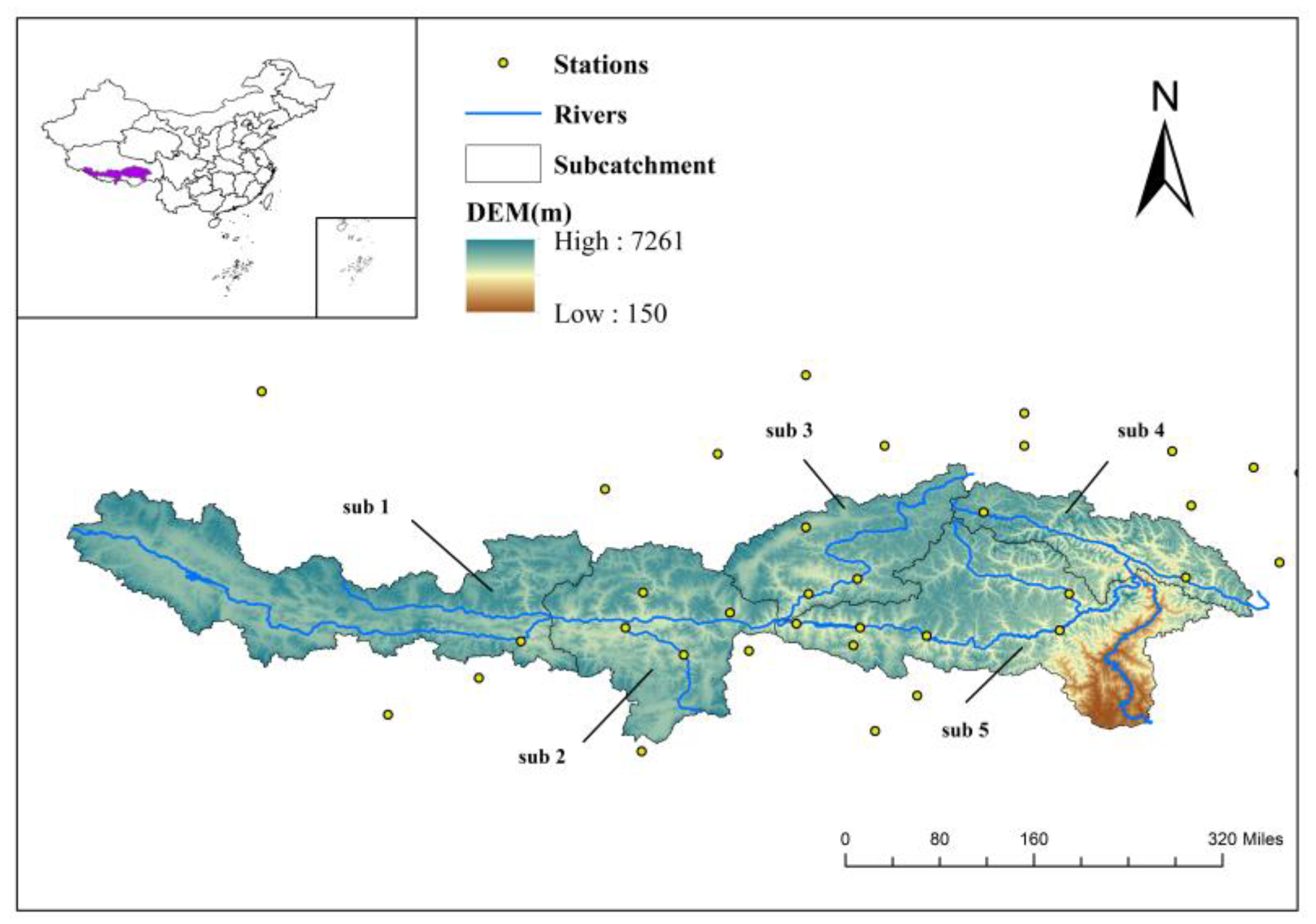
The Yarlung Zangbo River is the largest river on the Tibetan Plateau and one of the most important international rivers [43]. It originates from the Jemayangzong Glacier in southern Tibet and has a total length of 2229 km and its drainage area is 2.42 × 105 km² [44]. This river is one of the highest rivers in the world, with an average elevation of above 4600 m, and tilts from the west to the east, with an average slope of 2.6° [21]. The Yarlung Zangbo River has six major tributaries (the Dogxung Zangbo, Nyangqu, Lhasa, Nyang, Yigong Zangbo, and Purlung Zangbo Rivers). The locations of the YZRB and its tributaries are shown in Figure 1.

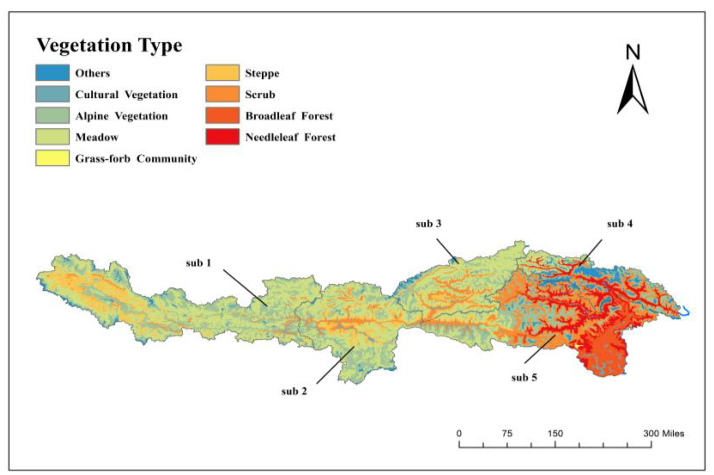
Because of the unique topographic characteristics and high altitude of the plateau, the vegetation and ecological environment of the YZRB are relatively fragile and complex [23] and show obvious changes from upstream to downstream [45]. According to the China Vegetation Atlas (Figure 2), the upstream region is located in an arid zone that is dominated by alpine grassland and meadows [46]. With decreasing elevation, the midstream transitions into a continental climate and is mainly covered by alpine grassland and meadows, and the cultivated vegetation slightly increases. The lower reaches of YZRB have a subtropical climate and are mainly covered by coniferous and broadleaf forests.

Yarlung Zangbo river has more than 130 tributaries, which is larger than 100 km², and its major tributaries include Nianchu River, Lhasa River, Nyang River, and Parlung Tsangpo. By considering the hydrological and vegetation similarity, which is shown in Figure 1 and Figure 2, the YLZB is divided into 5 subzones in the research. The area and vegetation conditions of the five subzones are shown in

Table 1. Name and area of the subzone.

Subzone	Watershed Name	Area (km2)
1	Upper reaches of the Yarlung Zangbo River	70,048
2	Nianchu River	43,741
3	Lhasa River	31,571
4	Parlung Zangbo	26,574
5	Nyang River	66,543
	Lower reaches of the Yarlung Zangbo River

and

Table 2. Proportion of different vegetation types in each subzone.

Subzone	1	2	3	4	5
Cultural Vegetation	0.29	2.49	1.41	0.11	2.43
Alpine Vegetation	32.71	26.26	20.81	26.65	21.8
Broadleaf Forest	0	0	0	0.38	15.73
Needle leaf Forest	0	0	0	19.23	16.13
Meadow	49.23	48.82	53.86	11.48	8.85
Steppe	11.86	12.79	7.69	0	1.6
Scrub	3.44	8.34	13.97	23.69	30.47
Others	2.48	1.29	2.25	18.46	3
total	100	100	100	100	100

.

2.2. Data Description

A quality-controlled NDVI remote sensing product (MOD13A3) is selected in this study, obtained from the observation of MODIS (Moderate Resolution Image Spectroradiometer) data provided by NASA, spanning 16 years (February 2000 to December 2015). MOD13A3 is the third level product, based on the secondary product, corrected the edge distortion (Bowtie effect) produced by the sensor imaging process. The spatial resolution of the product is 1.1 km × 1.1 km, while the time resolution is monthly. The data were processed into the Geostationary Earth Orbit Tag Image File Format (GEO TIFF) by MODIS Reprojection Tool (MRT) software and processed by ArcGIS projection splicing. The monthly mean air temperature and precipitation data covering 2000–2015 from 30 meteorological stations located in the YZRB were collected from the China Meteorological Data Network. The locations of the meteorological stations are shown in Figure 1.

2.3. Methodology

2.3.1. Random Forest

RF was first proposed by Breiman (2001) [47] as an ensemble learning method that can be used in both classification and regression tasks. The model is considered capable of dealing with small sample sizes and high-dimensional correlation relationships [47]. RF is also advantageous because of its robustness; it does not easily lead to overfitting or provide biased estimates when predictors that do not add information are used [48].

RF includes a group of classification and regression decision trees (CARTs) that are unpruned and generated by bootstrap sampling and random variable selection. The RF algorithm can be divided into the following steps. First, the training dataset is randomly extracted from the original dataset by bootstrap resampling. Second, the CARTs are established for each training set. Compared with the traditional CART method, RF selects random feature combinations to split each node, and each CART grows to the maximum extent without any pruning. Finally, the RF output is obtained by voting in classification mode or averaging in the regression mode of all of the CART predictions.

RF provides a built-in cross-validation process that occurs in parallel with the training procedure for the out-of-bag (OOB) samples, which are not chosen by the bootstrap process. RF can evaluate variable importance by randomly permuting these variables and observing the difference in model performance using OOB samples. At the end of procedure, RF obtains variable importance by averaging these differences, which is then normalized by the standard deviation.

2.3.2. Model Implementation and Validation

The RF is utilized to simulate the nonlinear relationship between the NDVI and climate factors in the 5 subzones. The monthly area-averaged NDVI datasets for each subzone were obtained by calculating the average values of each pixel. The monthly area-averaged precipitation and temperature of 5 subzones were obtained from actual data. For model development, the monthly average NDVI datasets and monthly area precipitation and temperature datasets of each subzone are divided into two datasets. The datasets from 2000 to 2009 were used for model calibration, and those from 2010 to 2015 were used for model validation.

Two machine learning models, ANN and SVM, which were previously used for NDVI prediction [49,50], were selected to compare with RF performance. A three-layer back propagation (BP) ANN model was used in this research. The BP method has been the most widely used algorithm to design multiple layer neural networks, and has also been successfully used for NDVI prediction [16]. SVM was the first classification machine learning algorithm and was proposed by Vapnik, and then gradually derived to the regression algorithm [51]. SVM has been widely used for hydrological prediction, and most recently for NDVI prediction. In this research, SVM with linear kernel function was used, which has been widely used in former studies.

One of the most important steps in the development of machine learning prediction models is the choice of appropriate predictors. Due to the spatial heterogeneity of the vegetation in the YLZB, the relationships between the NDVI and climate factors are different in the 5 subzones. Therefore, it is important to choose appreciate climate factors as predictors in NDVI prediction. In previous studies, PCA and PAR were used for predictor selections of ANN and SVM models. For comparative study, here, PAR and PCA were both used for predictor selection of the ANN and SVM models [52]. For PCA, the climate factors are standardized by subtracting the mean from the original values and then dividing the results by the standard deviation of the original variables. The PCA method is then applied to the standardized climate factors to extract principal components (PCs) that are orthogonal. The obtained PCs preserve more than 90% of the variances that are selected as predictors. Then, the PCs are used in the ANN and SVM modeling, and these results are marked as, ANN-PCA and SVM-PCA. For PAR, climate factors with a partial correlation coefficient greater than 0.3 were selected as predictors, and the corresponding results are marked as ANN-PAR and SVM-PAR.

2.3.3. Model Evaluation Index

The mean absolute percentage error (MAE), Nash–Sutcliffe coefficient (NASH), root mean square errors (RMSE), and correlation coefficient (R) statistical indicators were used to assess the predictive performance of the ANN, SVM, and RF models. MAE, NASH, RMSE, and R were defined as:

$$NASH=1-\frac{{\displaystyle \sum _{i=1}^n{(Y_{i,obs}-Y_{i,sim})}^2}}{{\displaystyle \sum _{i=1}^n{(Y_{i,obs}-\overline{Y_{obs}})}^2}},$$

$$RMSE=\sqrt{\frac{{\displaystyle \sum _{i=1}^n{(Y_{i,obs}-Y_{i,sim})}^2}}{n}},$$

$$MAE=\frac{{\displaystyle \sum _{i=1}^n\left|Y_{i,obs}-Y_{i,sim}\right|}}{n},$$

$$r=\frac{{\displaystyle \sum _{i=1}^n[(Y_{i,obs}-\overline{Y_{obs}})(Y_{i,sim}-\overline{Y_{sim}})]}}{\sqrt{[{\displaystyle \sum _{i=1}^n{(Y_{i,obs}-\overline{Y_{obs}})}^2]}}\sqrt{[{\displaystyle \sum _{i=1}^n{(Y_{i,sim}-\overline{Y_{sim}})}^2]}}}$$

where $Y_{i,obs}$ is the measured NDVI value of the station, $\overline{Y_{obs}}$ is the mean of the observed NDVI value, $Y_{i,sim}$ is the vector of the simulated NDVI value, and $\overline{Y_{sim}}$ is the mean of the simulated NDVI value. In general, a higher NASH value indicates better model efficiency; in contrast, smaller RMSE, MAE, and R values indicate higher accuracy.

3. Results and Discussion

3.1. Spatial and Temporal Characteristics of the NDVI in the YZRB

The inter-annual variations of the NDVI, precipitation, and temperature on the subzone scale from 2000 to 2015 are shown in

Table 3. Rainfall, temperature and the Normalized Difference Vegetation Index (NDVI) perennial change rate.

Subzone	Precipitation (mm)	Temperature (°C)	NDVI
Sub1	−3.9	0.02	0.1 × 10−3
Sub2	−3.7	0.04	0.1 × 10−3
Sub3	−9.86	0.07	0.4 × 10−3
Sub4	−13.86	0.04	0.7 × 10−3
Sub5	−12.8	0.01	0.2 × 10−3
Total	−8.25	0.03	0.2 × 10−3

. The NDVI and temperature values showed a statistically insignificant increase, whereas the average precipitation of the Yarlung Zangbo River Basin significantly decreased from 528 mm in 2000 to 396 mm in 2015, with a total increase of 0.8 °C over the 16 years. This finding is consistent with the results of previous studies [26].

In the five subzones, NDVI gradually increased from upstream to downstream. The average annual growth of NDVI in the five subzones was 0.1 × 10⁻³, 0.1 × 10⁻³, 0.4 × 10⁻³, 0.7 × 10⁻³, and 0.2 × 10⁻³. The precipitation and temperature show similar trends. The average annual growth of precipitation was −3.9, −3.7, −9.86, −13.86, and −12.8; the average annual growth of temperature was 0.02, 0.04, 0.07, 0.04, and 0.01.

3.2. Predictors Selection

In order to determine the optimal predictors for NDVI prediction models, PCA and PAR were used to analyze the relationships between NDVI and precipitation/temperature at different lead times. The results are shown in

Table 4. Contribution and cumulative contribution rates for selected principal components.

Subzone PCA		T0	P0	T1	P1	T2	P2	T3	P3
sub1	Contribution rate	0.46	0.26	0.14	0.06	0.03	0.03	0.01	0.01
	Cumulative contribution rate	0.46	0.72	0.86	0.92	0.95	0.98	0.99	1.00
sub2	Contribution rate	0.56	0.27	0.05	0.05	0.03	0.02	0.01	0.01
	Cumulative contribution rate	0.56	0.83	0.88	0.93	0.96	0.98	0.99	1.00
sub3	Contribution rate	0.59	0.19	0.06	0.05	0.04	0.03	0.03	0.01
	Cumulative contribution rate	0.59	0.78	0.84	0.89	0.93	0.96	0.99	1.00
sub4	Contribution rate	0.58	0.24	0.05	0.05	0.03	0.03	0.01	0.01
	Cumulative contribution rate	0.58	0.82	0.87	0.92	0.95	0.98	0.99	1.00
sub5	Contribution rate	0.57	0.20	0.08	0.06	0.04	0.03	0.01	0.01
	Cumulative contribution rate	0.57	0.77	0.85	0.91	0.95	0.98	0.99	1.00

T₀: Temperature of the month, P₀: rainfall of the month, T₁: temperature of the previous month, P₁: rainfall of the previous month, T₂: temperature of the first 2 months, P₂: rainfall of the last 2 months, T₃: temperature of the first 3 months, P₃: rainfall in the first 3 months.

and

Table 5. Partial correlation calculation results.

PAR	Sub1	Sub2	Sub3	Sub4	Sub5
T0	0.61	0.80	0.60	0.75	0.60
P0	0.56	0.78	0.58	0.66	0.57
T1	0.41	0.53	0.44	0.57	0.39
P1	−0.06	0.50	0.42	0.50	−0.06
T2	0.38	0.45	0.36	0.45	0.32
P2	−0.16	0.11	0.28	0.35	−0.11
T3	0.27	0.20	0.33	0.43	0.28
P3	−0.25	−0.20	−0.15	0.22	−0.25

T₀: Temperature of the month, P₀: rainfall of the month, T₁: temperature of the previous month, P₁: rainfall of the previous month, T₂: temperature of the first 2 months, P₂: rainfall of the last 2 months, T₃: temperature of the first 3 months, P₃: rainfall in the first 3 months.

, where Pn represents the average precipitation with a lead time n month, and Tn represents the average precipitation with a lead time n month. With reference to similar studies and the meteorological cycles [32,33,34,35], the maximum lead times were set to 6 months.

As shown in Table 4 and Table 5, the correlations between the NDVI and precipitation/temperature gradually decayed with the increase of lead time. The PCA results show that the precipitation and temperature whose lead time was shorter than 2 months had major impacts on the NDVI in these subzones. However, the PAR results varied in these subzones. In Sub1 and Sub5, the precipitation in the present month and temperature whose lead time was shorter than 2 months had major impacts on the NDVI. In Sub2, the precipitation whose lead time was shorter than 1 month and temperature whose lead time was shorter than 2 months had major impacts on the NDVI. In Sub3, the precipitation whose lead time shorter than 1 months and temperature whose lead time shorter than 3 months had major impacts on NDVI. In Sub4, the precipitation whose lead time was shorter than 2 months and temperature whose lead time was shorter than 3 months had major impacts on the NDVI. In general, the relationships between the NDVI and temperature were slightly closer than those between NDVI and precipitation in the five subzones.

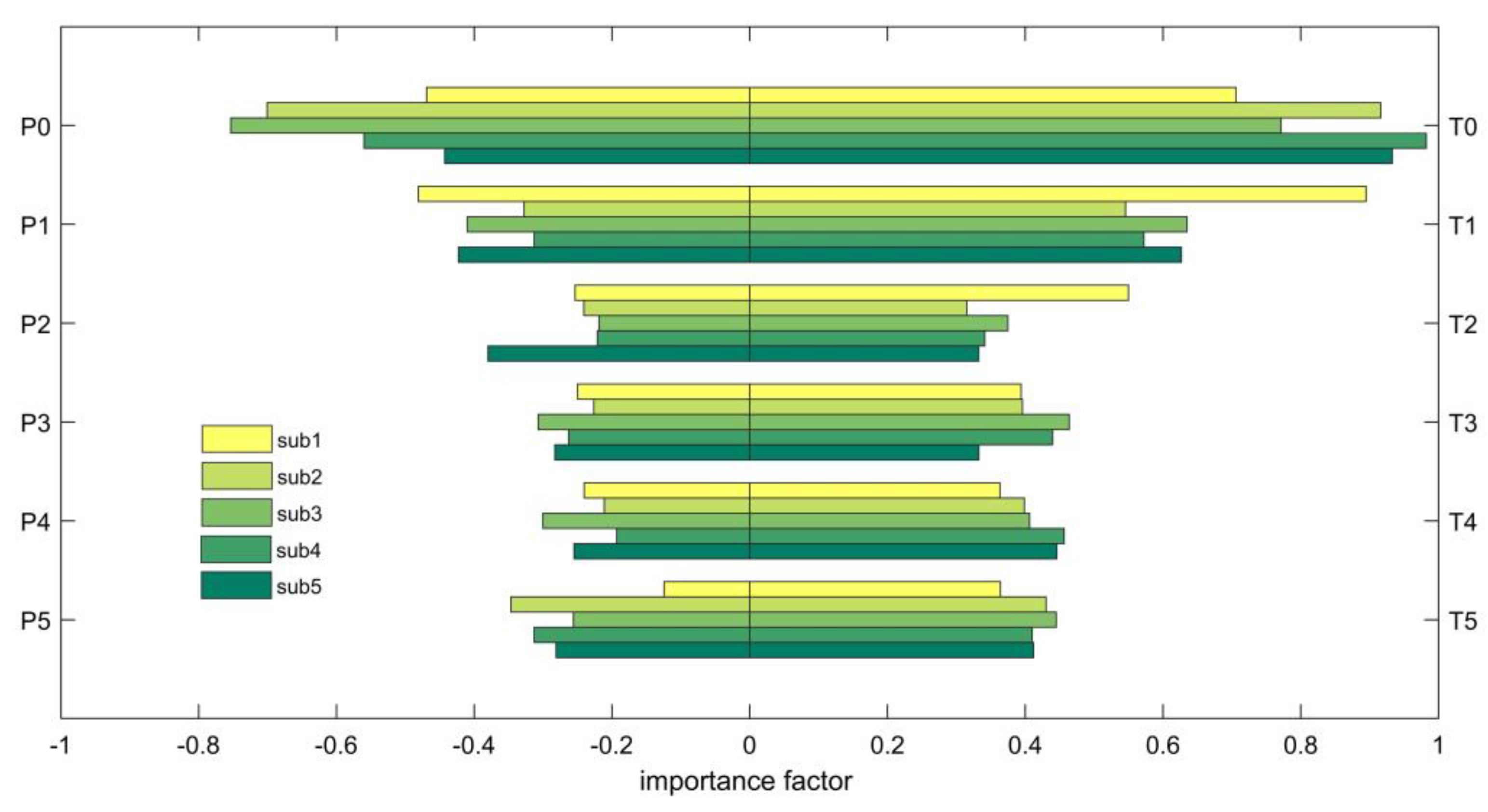
RF evaluates the relative contribution of each predictor using a built-in variable importance evaluation process. The importance of the precipitation/temperature at different lead times in these subzones are calculated and indicated in Figure 3. As illustrated in Figure 3, although the importance of precipitation and temperature gradually decreased, the increase in lead time and the decreases were not as significant as in the PCA and PAR results. This finding may indicate that RF can use all predictors without overfitting. Thus, the precipitation and temperature whose lead time was shorter than 6 months were used for RF modeling of the five subzones.

3.3. Comparative Study

The calibration and validation results of the RF and comparative models are summarized in

Table 6. Machine learning calculation results.

Subzone	Model	Calibration				Validation
		NASH	RMSE	MAEP	R	NASH	RMSE	MAEP	R
Sub1	ANN-PCA	0.68	0.03	0.02	0.84	0.67	0.03	0.03	0.86
	ANN-PAR	0.65	0.03	0.02	0.84	0.63	0.03	0.03	0.82
	SVM-PCA	0.90	0.02	0.01	0.95	0.87	0.02	0.01	0.95
	SVM-PAR	0.90	0.02	0.01	0.94	0.85	0.03	0.02	0.95
	RF	0.96	0.02	0.01	0.98	0.91	0.02	0.01	0.98
Sub2	ANN-PCA	0.74	0.03	0.03	0.91	0.73	0.04	0.03	0.92
	ANN-PAR	0.69	0.03	0.03	0.83	0.71	0.04	0.03	0.84
	SVM-PCA	0.90	0.02	0.02	0.95	0.91	0.02	0.01	0.95
	SVM-PAR	0.89	0.02	0.02	0.94	0.90	0.02	0.02	0.94
	RF	0.97	0.01	0.01	0.98	0.95	0.01	0.01	0.98
Sub3	ANN-PCA	0.78	0.05	0.05	0.94	0.77	0.05	0.04	0.94
	ANN-PAR	0.79	0.05	0.04	0.91	0.79	0.05	0.04	0.91
	SVM-PCA	0.91	0.04	0.03	0.95	0.89	0.04	0.03	0.95
	SVM-PAR	0.89	0.04	0.03	0.94	0.87	0.04	0.03	0.94
	RF	0.96	0.02	0.02	0.98	0.96	0.02	0.02	0.98
Sub4	ANN-PCA	0.75	0.05	0.04	0.90	0.75	0.05	0.04	0.89
	ANN-PAR	0.71	0.05	0.04	0.84	0.67	0.06	0.05	0.82
	SVM-PCA	0.85	0.04	0.03	0.92	0.82	0.04	0.03	0.92
	SVM-PAR	0.79	0.05	0.04	0.88	0.77	0.05	0.04	0.88
	RF	0.94	0.03	0.02	0.97	0.89	0.03	0.03	0.97
Sub5	ANN-PCA	0.78	0.04	0.03	0.89	0.72	0.05	0.04	0.87
	ANN-PAR	0.72	0.05	0.04	0.86	0.67	0.05	0.04	0.83
	SVM-PCA	0.84	0.04	0.03	0.92	0.73	0.05	0.03	0.92
	SVM-PAR	0.78	0.04	0.04	0.89	0.68	0.05	0.03	0.89
	RF	0.92	0.03	0.02	0.96	0.83	0.04	0.03	0.96

.

The results show that RF was superior to the comparative models in the calibration and validation periods. The NASH RF values for the five subzones were 0.96, 0.97, 0.96, 0.94, and 0.92 in the calibration period, and 0.91, 0.95, 0.96, 0.89, and 0.83 in the validation period. All of the measured criteria were superior to those of the compared models (ANN and SVM).

The results of the two-parameter selection were also compared between the ANN and SVM models. PCA was superior to PAR for both the ANN and SVM models. For the ANN models, the average RMSE and MAE were similar in both the calibration and validation periods. However, the average NASH and R of the results using PAR were superior to those of the PCA by 0.03 and 0.04 in the calibration period, and 0.03 and 0.05 in the validation period, respectively. For the SVM models, the average NASH and R increased by 0.03 and 0.02 in the calibration period, and 0.03 and 0.02 in the validation period, respectively. The average RMSE and MAE decreased by 0.002 and 0.004 in the calibration period, and 0.004 and 0.006 in validation period, respectively. Therefore, PCA was advantageous over PAR, with increases of NASH and R, and decreases of RMSE and MAE.

4. Conclusions

As a key component of ecohydrological processes, vegetation conditions influence the efficiency of plant water use and potentially affect water resources. Therefore, investing the changes of vegetation conditions and exploring the vegetation responses to climate changes will provide essential information for regional water resource management [53,54]. Combining with climate models, NDVI prediction models can assess the effects of future drought events [10]. As a covariate with other environmental variables, NDVI prediction models will also provide essential information for irrigation management [15] and soil-loss-prone area identification [12,13], etc. By exploring the vegetation condition changes of the YZRB and their relationship with climatic factors, we proposed an NDVI prediction model based on RF with area-averaged precipitation and temperature as predictors. The monthly rainfall and temperature observations from 30 meteorological stations in the YZRB and the MODIS NDVI datasets from 2000 to 2015 were selected to calibrate and validate the proposed model. The RF results were also compared with those of ANN and SVM models. The primary conclusions are as follows:

• RF successfully simulated the relationship between NDVI and climatic factors. The NASH coefficients of the proposed model during the calibration period in the five subzones were all higher than 0.9, and those during the verification period were all higher than 0.8. Among the five tested models, RF showed the highest model efficiency in both the calibration and validation periods among all compared models.
• RF showed advantages for predictor selection. The built-in variable importance evaluation allowed RF to select predictors without additional selection methods, such as PAR and PCA. Moreover, the numbers of predictors were greatest for RF among the compared models. RF showed robustness for modeling, because it could take full advantage of all predictor and avoid overfitting.
• PCA and PAR were used to analyze the factors that affect the NDVI in YZRB subzones. The results show that the rainfall and temperature of the first 3 months had significant impacts on NDVI, and temperature had a greater influence than rainfall in most of the subzones.

Because of sparse meteorological networks, this research was conducted on a subzone scale. In the future, we will try to explore the relationships between NDVI and climatic factors at a higher resolution with gridded meteorological observations, which will be more applicable for integrated water resource management. The adoption of more vegetation indices, such as leaf area index (LAI), is another important direction.

References

- Che, M.; Chen, B.; Innes, J.L.; Wang, G.; Dou, X.; Zhou, T.; Zhang, H.; Yan, J.; Xu, G.; Zhao, H. Spatial and temporal variations in the end date of the vegetation growing season throughout the Qinghai–Tibetan Plateau from 1982 to 2011. Agric. For. Meteorol. 2014, 189, 81–90. [Google Scholar] [CrossRef]
- Nouri, H.; Anderson, S.; Sutton, P.; Beecham, S.; Nagler, P.; Jarchow, C.J.; Roberts, D.A. NDVI, scale invariance and the modifiable areal unit problem: An assessment of vegetation in the Adelaide Parklands. Sci. Total. Environ. 2017, 584, 11–18. [Google Scholar] [CrossRef] [PubMed]
- Lemordant, L.; Gentine, P.; Swann, A.L.S.; Cook, B.I.; Scheff, J. Critical impact of vegetation physiology on the continental hydrologic cycle in response to increasing CO2. Proc. Natl. Acad. Sci. USA 2018, 115, 4093–4098. [Google Scholar] [CrossRef] [PubMed] [Green Version]
- Yang, Y.; Piao, S. Variations in grassland vegetation cover in relation to climatic factors on the Tibetan Plateau. J. Plant Ecol. 2006, 30, 1–8. [Google Scholar]
- Zhong, L.; Ma, Y.; Salama, M.S.; Su, Z. Assessment of vegetation dynamics and their response to variations in precipitation and temperature in the Tibetan Plateau. J. Clim. Chang. 2010, 103, 519–535. [Google Scholar] [CrossRef]
- Jiang, D.; Fu, X.; Wang, K. Vegetation dynamics and their response to freshwater inflow and climate variables in the Yellow River Delta, China. J. Quatern Int. 2013, 304, 75–84. [Google Scholar] [CrossRef]
- Barbosa, H.A.; Kumar, T.L.; Silva, L.R.M. Recent trends in vegetation dynamics in the South America and their relationship to rainfall. J. Nat. Hazards 2015, 77, 883–899. [Google Scholar] [CrossRef]
- Bao, G.; Qin, Z.; Bao, Y.; Zhou, Y.; Li, W.; Sanjjav, A. NDVI-Based Long-Term Vegetation Dynamics and Its Response to Climatic Change in the Mongolian Plateau. Remote Sens. 2014, 6, 8337–8358. [Google Scholar] [CrossRef] [Green Version]
- Aguilar, C.; Zinnert, J.C.; Polo, M.J.; Young, D.R. NDVI as an indicator for changes in water availability to woody vegetation. Ecol. Indic. 2012, 23, 290–300. [Google Scholar] [CrossRef]
- Dutta, D.; Kundu, A.; Patel, N. Predicting agricultural drought in eastern Rajasthan of India using NDVI and standardized precipitation index. Geocarto Int. 2013, 28, 192–209. [Google Scholar] [CrossRef]
- Omute, P.; Corner, R.; Awange, J.; Corner, R. The use of NDVI and its Derivatives for Monitoring Lake Victoria’s Water Level and Drought Conditions. Water Resour. Manag. 2012, 26, 1591–1613. [Google Scholar] [CrossRef] [Green Version]
- Carvalho, D.F.D.; Durigon, V.L.; Antunes, M.A.H.; Almeida, W.S.D.; Oliveira, P.T.S.D. Predicting soil erosion using Rusle and NDVI time series from TM Landsat 5. Pesq. Agropec. Bras. 2014, 49, 215–224. [Google Scholar] [CrossRef] [Green Version]
- Singh, D.; Herlin, I.; Berroir, J.; Silva, E.; Meirelles, M.S. An approach to correlate NDVI with soil colour for erosion process using NOAA/AVHRR data. Adv. Space Res. 2004, 33, 328–332. [Google Scholar] [CrossRef]
- White, D.C.; Lewis, M.M.; Green, G.; Gotch, T.B. A generalizable NDVI-based wetland delineation indicator for remote monitoring of groundwater flows in the Australian Great Artesian Basin. Ecol. Indic. 2016, 60, 1309–1320. [Google Scholar] [CrossRef] [Green Version]
- Fu, B.; Burgher, I. Riparian vegetation NDVI dynamics and its relationship with climate, surface water and groundwater. J. Arid. Environ. 2015, 113, 59–68. [Google Scholar] [CrossRef]
- Huang, S.; Ming, B.; Leng, G.; Hou, B. A Case Study on a Combination NDVI Forecasting Model Based on the Entropy Weight Method. Water Resour. Manag. 2017, 31, 3667–3681. [Google Scholar] [CrossRef]
- Piao, S.; Wang, T.; Ciais, P.; Zhu, B.; Liu, J. Changes in satellite?derived vegetation growth trend in temperate and boreal Eurasia from 1982 to 2006. Glob. Chang. Boil. 2011, 17, 3228–3239. [Google Scholar] [CrossRef]
- Aldakheel, Y.Y. Assessing NDVI Spatial Pattern as Related to Irrigation and Soil Salinity Management in Al-Hassa Oasis, Saudi Arabia. J. Indian Soc. Remote Sens. 2011, 39, 171–180. [Google Scholar] [CrossRef]
- Li, H.; Liu, L.; Shan, B.; Xu, Z.; Niu, Q.; Cheng, L.; Liu, X.; Xu, Z. Spatiotemporal Variation of Drought and Associated Multi-Scale Response to Climate Change over the Yarlung Zangbo River Basin of Qinghai–Tibet Plateau, China. Remote Sens. 2019, 11, 1596. [Google Scholar] [CrossRef] [Green Version]
- Wang, X.; Zhong, X.; Fan, J. Assessment and spatial distribution of sensitivity of soil erosion in Tibet. J. Geogr. Sci. 2004, 14, 41–46. [Google Scholar] [CrossRef]
- Li, F.; Zhang, Y.; Xu, Z.; Teng, J.; Liu, C.; Liu, W.; Mpelasoka, F. The impact of climate change on runoff in the southeastern Tibetan Plateau. J. Hydrol. 2013, 505, 188–201. [Google Scholar] [CrossRef]
- Liu, Z.; Yao, Z.; Huang, H.; Wu, S.; Liu, G. Land use and climate changes and their impacts on runoff in The Yarlung Zangbo river basin. J. Land Degrad. Dev. 2014, 25, 203–215. [Google Scholar] [CrossRef]
- Li, H.; Li, Y.; Shen, W.; Li, Y.; Lin, J.; Lu, X.; Xu, X.; DeAngelis, D. Elevation-Dependent Vegetation Greening of the Yarlung Zangbo River Basin in the Southern Tibetan Plateau, 1999–2013. Remote Sens. 2015, 7, 16672–16687. [Google Scholar] [CrossRef] [Green Version]
- Han, X.; Zuo, D.; Xu, Z.; Cai, S.; Gao, X. Analysis of vegetation condition and its relationship with meteorological variables in the Yarlung Zangbo River Basin of China. Proc. Int. Assoc. Hydrol. Sci. 2018, 379, 105–112. [Google Scholar] [CrossRef] [Green Version]
- Liu, X.; Xu, Z.; Peng, D. Spatio-Temporal Patterns of Vegetation in the Yarlung Zangbo River, China during 1998–2014. J. China Rural Water Hydropower 2019, 11, 1–11. (In Chinese) [Google Scholar] [CrossRef] [Green Version]
- Sun, W.; Wang, Y.; Fu, Y.H.; Xue, B.; Wang, G.; Yu, J.; Zuo, D.; Xu, Z. Spatial heterogeneity of changes in vegetation growth and their driving forces based on satellite observations of the Yarlung Zangbo River Basin in the Tibetan Plateau. J. Hydrol. 2019, 574, 324–332. [Google Scholar] [CrossRef]
- Di, L.; Rundquist, D.C.; Han, L. Modelling relationships between NDVI and precipitation during vegetative growth cycles. Int. J. Remote Sens. 1994, 15, 2121–2136. [Google Scholar] [CrossRef]
- Braswell, B.; Schimel, D.S.; Linder, E.; Moore, B. The Response of Global Terrestrial Ecosystems to Interannual Temperature Variability. Science 1997, 278, 870–873. [Google Scholar] [CrossRef]
- Tian, F.; Fensholt, R.; Verbesselt, J.; Grogan, K.; Horion, S.; Wang, Y. Evaluating temporal consistency of long-term global NDVI datasets for trend analysis. Remote Sens. Environ. 2015, 163, 326–340. [Google Scholar] [CrossRef]
- Wang, J.; Rich, P.M.; Price, K.P. Temporal responses of NDVI to precipitation and temperature in the central Great Plains, USA. Int. J. Remote Sens. 2003, 24, 2345–2364. [Google Scholar] [CrossRef]
- Iwasaki, H. NDVI prediction over mongolian grassland using Gsmap Precipitation Data and Jra-25/jcdas Temperature Data. J. Arid Environ. 2009, 73, 557–562. [Google Scholar] [CrossRef]
- Meng, B.; Gao, J.; Liang, T.; Cui, X.; Ge, J.; Yin, J.; Feng, Q.; Xie, H. Modeling of Alpine Grassland Cover Based on Unmanned Aerial Vehicle Technology and Multi-Factor Methods: A Case Study in the East of Tibetan Plateau, China. Remote Sens. 2018, 10, 320–339. [Google Scholar] [CrossRef] [Green Version]
- Kang, L.; Di, L.; Deng, M.; Yu, E.; Xu, Y. Forecasting vegetation index based on vegetation-meteorological factor interactions with artificial neural network. In Proceedings of the 2016 Fifth International Conference on Agro-Geoinformatics (Agro-Geoinformatics), Tianjin, China, 18–20 July 2016; pp. 1–6. [Google Scholar]
- Nay, J.; Burchfield, E.; Gilligan, J.M. A machine-learning approach to forecasting remotely sensed vegetation health. Int. J. Remote Sens. 2017, 39, 1800–1816. [Google Scholar] [CrossRef]
- Asoka, A.; Mishra, V.; Akarsh, A. Prediction of vegetation anomalies to improve food security and water management in India. Geophys. Res. Lett. 2015, 42, 5290–5298. [Google Scholar] [CrossRef] [Green Version]
- Thukaram, D.; Khincha, H.; Vijaynarasimha, H. Artificial Neural Network and Support Vector Machine Approach for Locating Faults in Radial Distribution Systems. IEEE Trans. Power Deliv. 2005, 20, 710–721. [Google Scholar] [CrossRef] [Green Version]
- Feng, X.W.; Hang, L.M.; Shen, B. Comparative study on multivariate linear regression and BP neural network model in the prediction of flood volume. J. Water Resour. Water Eng. 2017, 28, 123–126. (In Chinese) [Google Scholar]
- Kaufmann, R.K.; Zhou, L.; Myneni, R.; Tucker, C.J.; Slayback, D.; Shabanov, N.V.; Pinzon, J. The effect of vegetation on surface temperature: A statistical analysis of NDVI and climate data. Geophys. Res. Lett. 2003, 30, 2147–2150. [Google Scholar] [CrossRef] [Green Version]
- Ge, J.; Meng, B.; Liang, T.; Feng, Q.; Gao, J.; Yang, S.; Huang, X.; Xie, H. Modeling alpine grassland cover based on MODIS data and support vector machine regression in the headwater region of the Huanghe River, China. Remote Sens. Environ. 2018, 218, 162–173. [Google Scholar] [CrossRef]
- Hsu, C.; Chang, C.; Lin, C. A practical guide to support vector classification. J. Bju Int. 2008, 101, 1396–1400. [Google Scholar]
- Binren, X.; Yuanyuan, W. Spatial statistics of TRMM precipitation in the Tibetan Plateau using random forest algorithm. J. Remote Sens. Land Resour. 2018, 30, 181–188. [Google Scholar]
- Tongtiegang, Z.; Dawen, Y.; Ximing, C.; Yong, C. Predict seasonal low flows in the upper Yangtze River using random forests model. J. Hydroelectr. Eng. 2015, 31, 19–27. (In Chinese) [Google Scholar]
- Lehnert, L.; Meyer, H.; Wang, Y.; Miehe, G.; Thies, B.; Reudenbach, C.; Bendix, J. Retrieval of grassland plant coverage on the Tibetan Plateau based on a multi-scale, multi-sensor and multi-method approach. Remote Sens. Environ. 2015, 164, 197–207. [Google Scholar] [CrossRef]
- Ma, Y.; Yang, Y.; Han, Z.; Tang, G.; Maguire, L.; Chu, Z.; Hong, Y. Comprehensive evaluation of Ensemble Multi-Satellite Precipitation Dataset using the Dynamic Bayesian Model Averaging scheme over the Tibetan plateau. J. Hydrol. 2018, 556, 634–644. [Google Scholar] [CrossRef]
- Chen, B.; Li, H.; Cao, X.; Shen, W.; Jin, H. Vegetation Pattern and Spatial Distribution of NDVI in the Yarlung Zangbo River Basin of China. J. Desert Res. 2015, 35, 120–128. (In Chinese) [Google Scholar]
- Shen, M.; Piao, S.; Cong, N.; Zhang, G.; Jassens, I.A. Precipitation impacts on vegetation spring phenology on the Tibetan Plateau. Glob. Chang. Boil. 2015, 21, 3647–3656. [Google Scholar] [CrossRef] [PubMed] [Green Version]
- Breiman, L. Random forests. Mach. Learn. 2001, 45, 5–32. [Google Scholar] [CrossRef] [Green Version]
- Biau, G.; Scornet, E. A random forest guided tour. TEST 2016, 25, 197–227. [Google Scholar] [CrossRef] [Green Version]
- Baez-Villanueva, O.M.; Zambrano-Bigiarini, M.; Beck, H.E.; McNamara, I.; Ribbe, L.; Nauditt, A.; Birkel, C.; Verbist, K.; Giraldo-Osorio, J.D.; Thinh, N.X. RF-MEP: A novel Random Forest method for merging gridded precipitation products and ground-based measurements. Remote Sens. Environ. 2020, 239, 111606. [Google Scholar] [CrossRef]
- Were, K.; Bui, D.T.; Øystein, B.D.; Singh, B.R. A comparative assessment of support vector regression, artificial neural networks, and random forests for predicting and mapping soil organic carbon stocks across an Afromontane landscape. Ecol. Indic. 2015, 52, 394–403. [Google Scholar] [CrossRef]
- Pan, X.C. Application of SCA-SVM to annual runoff wet-dry identification. J. China Three Gorges Univ. 2016, 38, 6–11. (In Chinese) [Google Scholar]
- Pang, B.; Yue, J.; Zhao, G.; Xu, Z. Statistical Downscaling of Temperature with the Random Forest Model. Adv. Meteorol. 2017, 2017, 1–11. [Google Scholar] [CrossRef] [Green Version]
- Peng, D.; Du, Y. Comparative analysis of several Lhasa River basin flood forecast models in Yarlung Zangbo River. In Proceedings of the 2010 4th International Conference on Bioinformatics and Biomedical Engineering, Chengdu, China, 18–20 June 2010; pp. 1–4. [Google Scholar]
- Zhang, J.; Ren, Z. Responses of vegetation changes in growing season to precipitationin Yarlung Zangbo River Basin. J. Soil Water Conserv. 2015, 2, 209–212. [Google Scholar]
Figure 1.
Location of the Yarlung Zangbo River Basin (YZRB) and its five subzones.
Figure 2.
Vegetation conditions map of the YZRB.
Figure 3.
Important factors (rainfall and temperature) in different months.