The Effect of Habitat Structure Boulder Spacing on Near-Bed Shear Stress and Turbulent Events in a Gravel Bed Channel


Civil and Environmental Engineering Department, Clarkson University, Potsdam, NY 13699, USA
*
Author to whom correspondence should be addressed.
Water 2020, 12(5), 1423; https://doi.org/10.3390/w12051423
Submission received: 10 April 2020
/
Revised: 12 May 2020
/
Accepted: 14 May 2020
/
Published: 16 May 2020
(This article belongs to the Special Issue A Systems Approach for River and River Basin Restoration)
Abstract
:This study experimentally investigated the effect of boulder spacing and boulder submergence ratio on the near-bed shear stress in a single array of boulders in a gravel bed open channel flume. An acoustic Doppler velocimeter (ADV) was used to measure the instantaneous three-dimensional velocity components. Four methods of estimating near-bed shear stress were compared. The results suggested a significant effect of boulder spacing and boulder submergence ratio on the near-bed shear stress estimations and their spatial distributions. It was found that at unsubmerged condition, the turbulent kinetic energy (TKE) and modified TKE methods can be used interchangeably to estimate the near-bed shear stress. At both submerged and unsubmerged conditions, the Reynolds method performed differently from the other point-methods. Moreover, a quadrant analysis was performed to examine the turbulent events and their contribution to the near-bed Reynolds shear stress with the effect of boulder spacing. Generally, the burst events (ejections and sweeps) were reduced in the presence of boulders. This study may improve the understanding of the effect of the boulder spacing and boulder submergence ratio on the near-bed shear stress estimations of stream restoration practices.
1. Introduction
Bed shear stress plays a determinant role in the incipient motion of sediment. The bed shear stress has been the focus of many studies in both laboratory flumes and rivers. The majority of the existing studies were conducted in the flumes due to the controlled flow and bed conditions. However, the field investigation on the measuring of the bed shear stress is relatively limited. The direct measurements on the bed shear stress were often conducted by using the shear plate [1,2,3,4,5]. The indirect measurement of the bed shear stress depends on the velocity in the inner layer, lower 20% of the flow depth [6]. The common approaches to calculate the bed shear stress include, but are not limited to, the reach-averaged bed shear [7], logarithmic law of the wall [8], drag force [9], Reynolds stress [10], and turbulent kinetic energy (TKE) methods [11]. In a laboratory study, the bed shear stress estimated from several methods were compared for a simple boundary layer and a complex flow [12]. It was found that the Reynolds and TKE methods showed the most appropriate results for a simple boundary layer and a complex flow, respectively [12]. In another study, Reynolds stress was calculated by using the double-averaged methodology based on Reynolds temporal and spatial averaging [13]. The study concluded that the maximum Reynolds stress could better represent the bed shear stress than the linearly extrapolated Reynolds stress profile [13]. In the field measurements, acoustic Doppler current profiler (ADCP) has been commonly used for the measurement of velocity profiles to provide estimates of shear stress [8,14,15]. The bed shear stress was estimated from the logarithmic law of the wall and depth-averaged velocity in the Lower Fraser River, Canada, by using obtained data from an ADCP [15]. The field investigation indicated that using depth-averaged velocity paired with the zero-velocity height based on bed grain size gives more reliable results on the shear stress than using the logarithmic law of the wall [8].
The in-stream habitat structure boulder is one of the most favorable measures for river/stream restoration projects. The Natural Resources Conservation Service (NRCS 1998) demonstrated different utilization of boulders for channel restoration designs [16]. The boulders in the channel enhance the flow heterogeneity and modify the sediment transport process such that fish habitat, channel bed/bank stabilities, and water quality are improved [17]. Five stream restoration projects have been performed by using boulders to shed light on the benefits of adding boulders for local hydraulic conditions, thermal conditions, and total transient storage [18]. Although stream/river restoration has become a worldwide phenomenon and booming enterprise [19], our knowledge of the flow hydrodynamics associated with boulders is very limited [17]. The understanding of the impact that in-stream boulders bring about on the bed shear stress and fish habitat requires systematic investigation. The quantitative description of how the boulder spacing and boulder submergence ratios affect the bed shear stress, which is the key factor for bed sediment transport, would be useful for the channel restoration design.
The few existing studies measuring the bed shear stress with a disruption such as boulders shed light on its impact on flow configurations [20,21,22,23,24,25,26] and sediment transport [23,27,28,29]. Boulders have been documented to create spatial variability in bed shear stress [28,30,31,32]; and the presence of boulders decreases the sediment transport capacity [33,34]. The flume measurements over the gravel bed indicated that near-bed flow plays a key role in the flow structure fed into the outflow, and the increasing Reynolds number promotes large-scale flow structures [26]. The experimental studies demonstrated that a single boulder or an array of boulders affect the mean and turbulent flow characteristics [22,24,30]. It has been reported that the presence of boulder deaccelerates flow and leads to a significant deviation of streamwise mean velocity from the classic logarithmic law [22]. A boulder array generally leads to a decreased total bedload transport rate due to the reduction of available grain shear stress caused by the boulder form drag [24]. Several bed load equations have been proposed for boulder-bed channels considering the effects of sediment availability, boulder protrusion, bed roughness, the variability of shear stress, and boulder spacing [28,29]. Moreover, the boulder submergence ratio can be considered as a key parameter that affects the mean and turbulent flow characteristics as well as the local sediment transport patterns [23,30,35]. For a partially submerged flow, an array of boulders may reduce 5–20 times the bedload rate compared to conditions without boulders [36]. It has been reported that under the unsubmerged and fully submerged conditions, the deposition of the sediment may significantly vary downstream and upstream of boulders [35].
From the turbulence aspect, many recent studies have primarily focused on the effects of coherent flow structures (i.e., turbulent bursting events) on the flow field and sediment transport with or without the presence of large roughness elements such as boulders [28,37,38,39,40,41,42]. Turbulent events may affect bedload and suspended load sediment movement, as well as fish behavior and swimming performance, which can be of great importance in the design of natural fish habitat structures [43]. Turbulent events as a cycle of ejections, sweeps, outward, and inward interactions contribute to the Reynolds shear stress. Ejections transfer slow-moving fluid into the outer layer while sweeps bring high-momentum fluid into the bed region [44]. Ejection events have been reported important in sediment entrainment into the water column, while sweeps are associated with bedload transport [40]. Quadrant analysis has been widely used to highlight the significance of turbulent events, specifically around large roughness elements [21,36,38,45]. However, there is still a lack of knowledge on the turbulent events variation and their contribution to the Reynolds shear stress under different boulder spacing and submergence ratios.
This study is motivated by the need to improve our understanding of how the boulder spatial distribution, which is frequently employed in stream restoration practices, affects the near-bed shear stress and its estimations. This study experimentally investigates the effects of boulder spacing and boulder submergence ratio on the near-bed shear stress in a flume with a gravel bed. Four different methods were used to estimate the reach-averaged near-bed shear stress and its spatial distribution. Besides, the performance of methods was compared with each other. Moreover, dominant turbulent events and their contribution to the near-bed Reynolds shear stress was studied through a quadrant analysis to deepen the understanding of near-bed turbulence under varying boulder spacing and submergence ratio.
2. Materials and Methods
2.1. Experimental Setup
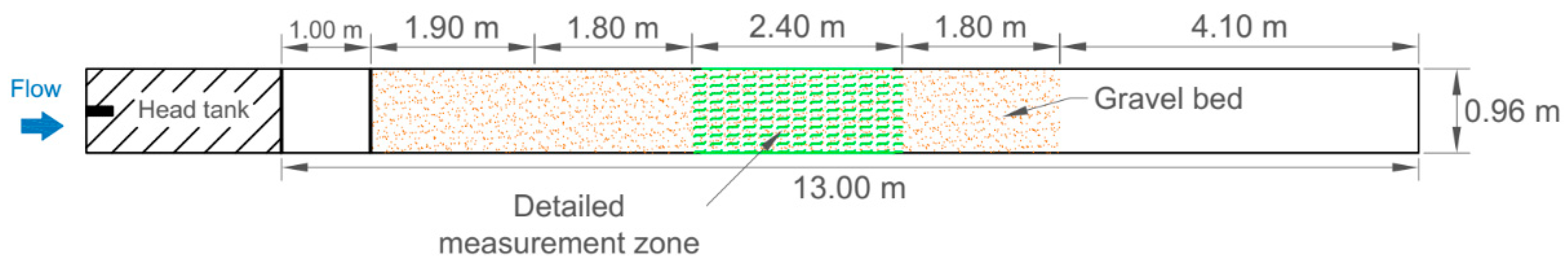
Experiments were conducted in the Ecohydraulics Flume, a 13.0 m long, 0.96 m wide, water-recirculating flume with a gentle slope (S0) of 0.5% located in the Water Resources Engineering Laboratory at Clarkson University. Measurements were taken in a section with a length of 2.40 m located 3.80 m downstream from the flume entrance to ensure that the turbulent flow is hydraulically fully developed. Figure 1 shows a scheme of the flume. Natural semi-spherical shape boulders with an equivalent diameter (D) of 12.50 cm were used as large roughness elements. Experiments were carried out over a gravel bed with d90 = 27.50 mm, d50 = 17.21 mm, and d10 = 9.37 mm, where dp refers to the grain size for which p% of particle sizes are finer. The critical bed shear stress for the median sediment size (d50) was calculated according to [46] formula, and it was 12.38 N/m2, at which incipient sediment motion takes place. As projected, no sediment movement was observed at any set of experiments.
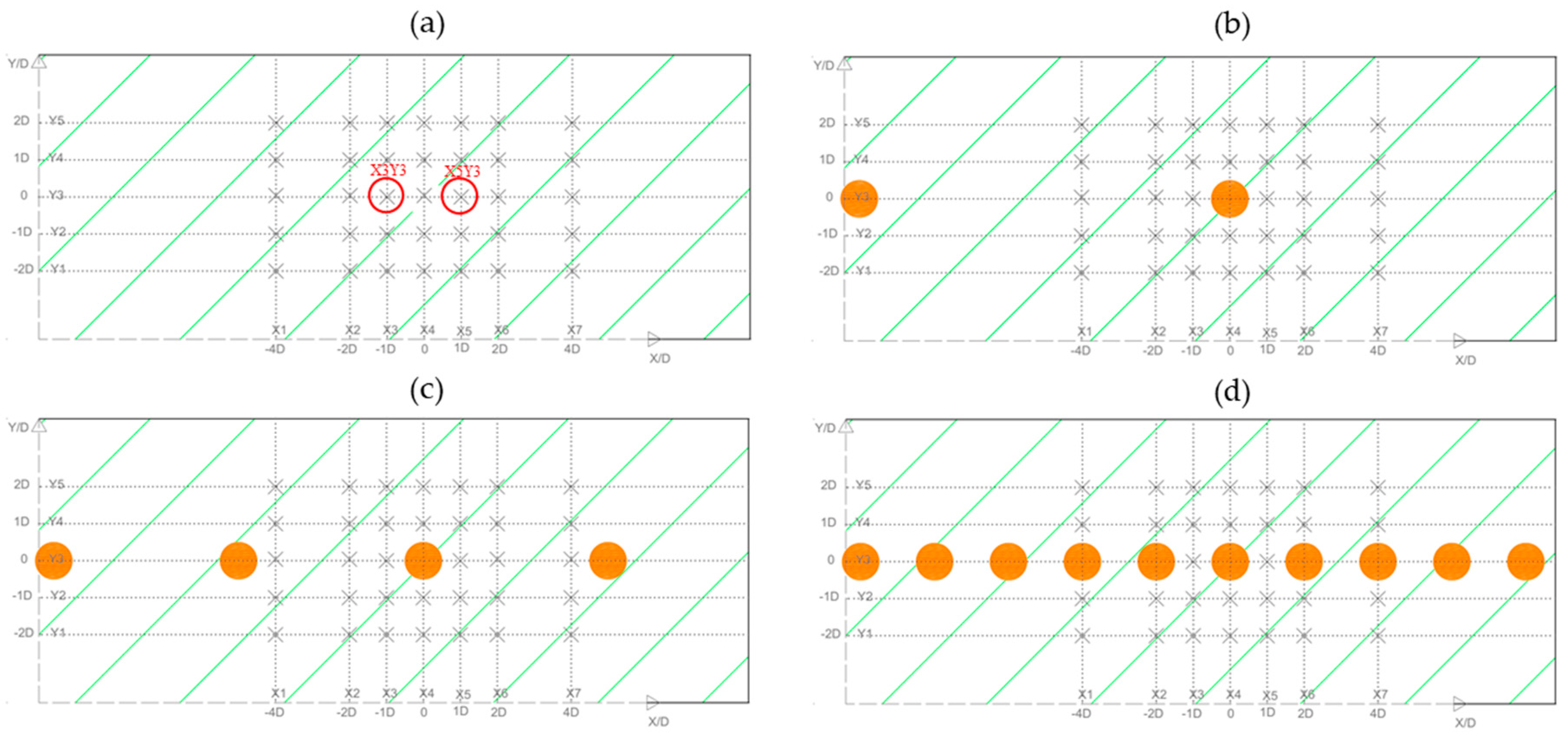
Four series of experiments (hereafter called scenarios) were designed with boulder-to-boulder spacing (from center to center) as a varying parameter to represent different flow regimes. Covered boulder-to-boulder spacing was infinity (no boulder), 10D (large spacing), 5D (medium spacing), and 2D (small spacing). The large and medium boulder spacing referred to an isolated flow regime while the small boulder spacing corresponded to a wake-interference or even a skimming flow regime [38]. Table 1 lists four scenarios and the hydraulic parameters associated with each scenario. Each scenario was conducted at 60 L/s and 100 L/s flow rates. Boulders were unsubmerged at 60 L/s with a submergence ratio (H/D) between 0.73 and 0.78, while at 100 L/s, boulders were fully submerged with a submergence ratio between 1.25 and 1.32 (Table 1). Figure 2 illustrates the measurement points and position of boulders in each scenario in the measurement zone. For the boulder-scenarios, the boulders were placed along the centerline of the channel in a single straight array. First, the central boulder at point X4Y3 was placed; afterward, the other boulders were arranged relative to the central boulder. A total of 35 measurement points were selected covering an area from −4D to 4D (relative to the central boulder in the measurement zone) in the streamwise direction (x) and from −2D to 2D in the spanwise direction (y) of the central boulder. The distance of all the measurement points from the walls was greater than 10 cm to minimize the wall effects [28]. It is worth mentioning that 35 measurement points were measured for the no-boulder scenario; however, for the boulder-scenarios, some of the measurement points in the centerline of the boulders were blocked by the boulders. In addition, Figure 2 shows that the points immediately upstream and downstream of a boulder have an equal distance from the boulder; however, due to the irregularity in the boulder shape, these distances were not perfectly the same.
The velocity measurements were taken in a relative depth (z/H) around 0.20–0.25, at the beginning of the outer region of flow [47]. Although measurements closer to the bed are preferable, the use of such a relative depth to capture the near-bed flow characteristics has been justified in a similar study [42]. Additionally, acoustic Doppler velocimeter (ADV) measurement about 3 cm from the bed to acquire higher levels of accuracy within the turbulent flows has been recommended [48], a threshold that led to a z/H around 0.20–0.30 in this study.
2.2. Data Filtering
Three-dimensional instantaneous velocities were collected using a Vectrino probe (Nortek ADV) at a sampling rate of 25 Hz for three minutes to ensure statistical significance. Aliased points were despiked using a phase-space threshold filter proposed by [49]. This filter can produce clean signals in highly turbulent flows [50]. The manufacturer (Nortek) recommends COR ≥ 70% and SNR ≥ 15 dB for reliable turbulence measurements. However, in the case of high SNR values—a valid condition in this study with an average SNR value of greater than 50 dB—COR values less than 70% can still provide reliable data [51]. As suggested by [52], COR values less than 70% in the turbulent flows are not necessarily an indicator of the low quality. They applied COR ≥ 50% and SNR ≥ 10 dB to investigate the turbulent characteristics around a cluster microform [52]. It also has been shown that for the flow over a rough bed, if at least 70% of data remain after applying a filtering scheme, the Reynolds stress could be measured with a minimum COR of 40% [53]. Following these suggestions, a filtering scheme with COR ≤ 65% and SNR ≤ 20 dB was applied to filter out poor quality data. For the points in location X5Y3 (marked in Figure 2a) at 100 L/s flow rate, a COR of 55% was applied due to the higher turbulence in this point and a significant loss of data in case of applying the main filtering scheme. Such criteria resulted in the remaining 77.1% of data indicating an acceptable portion of data for further analysis. Another possible source of error in ADV data is the Doppler noise, which may affect the turbulence parameters [54]. When the noise level is low, it is expected that the velocity spectra follow the Kolmogorov’s −5/3 law by exhibiting a −5/3 slope in the inertial subrange of the velocity spectra [54]. Therefore, as an additional check (also suggested by [50] for highly turbulent flows), the velocity spectra of the measured time series were visually inspected to remove noisy time series with a flat or negative slope in the inertial subrange. None of the points were rejected based on this criterion.
2.3. Calculation of Bed Shear Stress
The first main method to calculate the bed shear stress is the reach-averaged method as below [12]:
where is bed shear stress, is water density, is gravitational acceleration, and R is channel hydraulic radius. Although this method gives a rough estimation of bed shear stress, its performance is questionable, specifically in the presence of boulders, because it is not able to estimate the local variation of the bed shear stress [12].
Bed shear stress can be estimated directly through the Reynolds shear stress [12]:
where and are the instantaneous velocity fluctuations of the streamwise and vertical components, respectively. The bar sign over indicates a time-averaged value. This method is sensitive to the deviations from a two-dimensional uniform flow [12].
Another method is the turbulence kinetic energy (TKE) method as below [12]:
where is the instantaneous velocity fluctuation of the spanwise component and is a constant equal to 0.19 [11].
The modified TKE method only uses the vertical component of the velocity fluctuations due to the smaller noise of the measurement instrument in this direction [11]. Therefore, it can be written as below [12]:
where is a constant equal to 0.9 [11].
Equations (1)–(4) were used to calculate the near-bed shear stress for all the conducted scenarios in this study. Equation (1) only requires the reach hydraulic data while Equations (2)–(4) use the measured data from a single point and are referred to as point-methods in this study.
2.4. Quadrant Analysis
In a quadrant analysis, the velocity fluctuations are decomposed to four quadrants based on their signs [38]:
- Quadrant 1: outward interactions ()
- Quadrant 2: ejection events ()
- Quadrant 3: inward interactions ()
- Quadrant 4: sweep events ().
To remove insignificant events, a hole region in the () plane can be defined to exclude points within this region. Hole size, H, is a parameter to define the expansion of the hole region as below [55]:
Clearly, a larger hole size means the remaining of more significant events. Many studies have selected a hole size greater than one to distinguish significant events [36,56,57,58,59]. Therefore, in this study, a hole size of 2 was selected to distinguish events with a higher magnitude. Points X3Y3 and X5Y3, the common points in all the scenarios (marked in Figure 2a), were selected for a quadrant analysis. The joint frequency distribution of the normalized velocity fluctuations was found for each point. To find the contribution of each quadrant to the Reynolds shear stress, the stress fraction parameter of each quadrant, was found as below [38]:
where shows the quadrant number ( = 1, 2, 3, 4), is the total duration of the measurement and is a conditional function to detect events in each quadrant for a given hole number as below [38]:
The total portion of each turbulent event, , as a representative of the frequency of turbulent events can be determined as below [38]:
3. Results and Discussion
3.1. Near-Bed Shear Stress
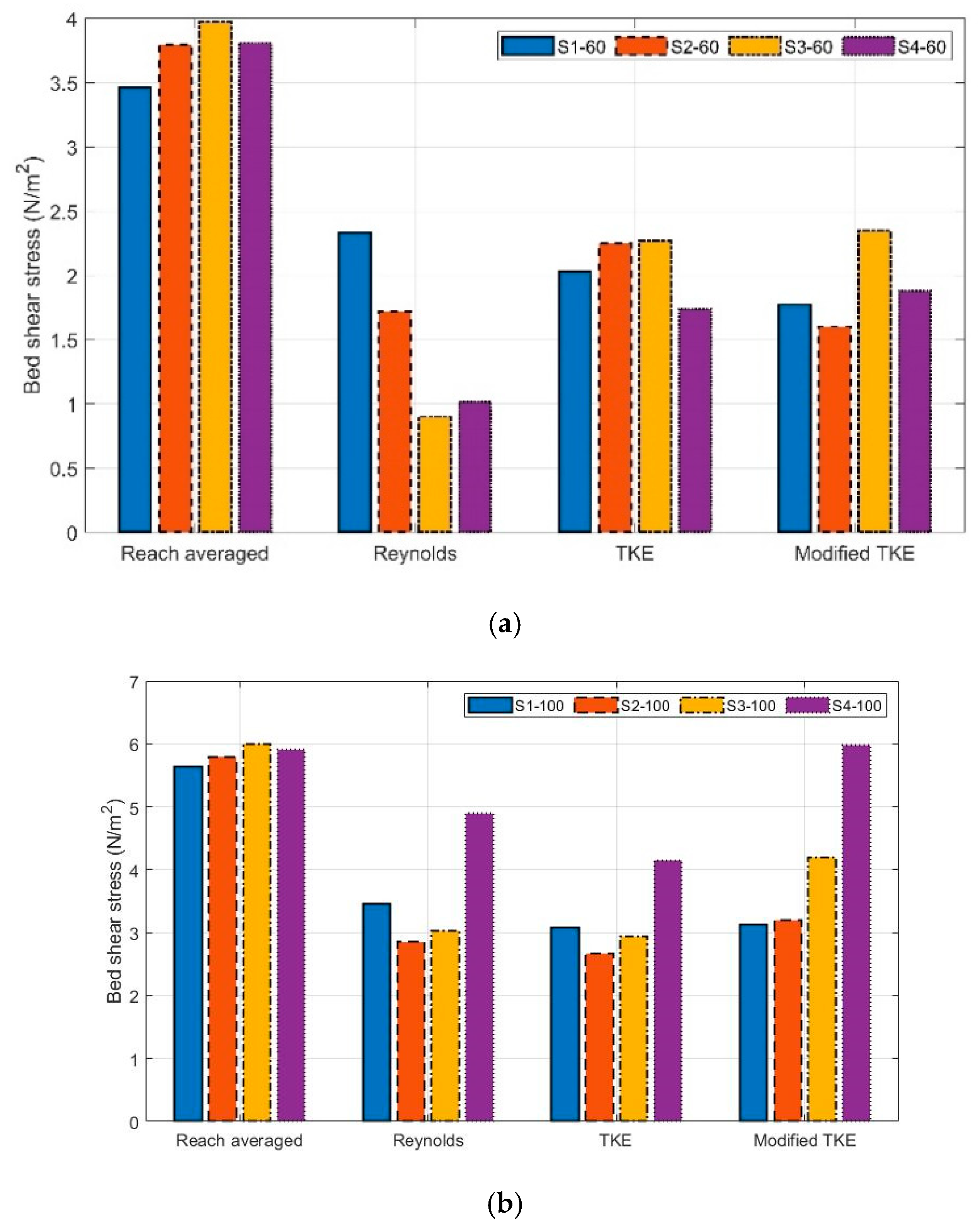
Equations (1)–(4) were used to calculate the reach-averaged near-bed shear stress for each scenario. Equation (1) gives a single value as the reach-averaged shear stress, but for the point-methods, the average of shear stresses at all the measurement points was calculated as the reach-averaged near-bed shear stress. Figure 3 shows the reach-averaged near-bed shear stress for each method and scenario. The near-bed shear stress estimations using the reach-averaged method (Equation (1)) before adding boulders were 3.46 and 5.63 N/m2 for the S1-60 and the S1-100 scenarios, respectively. These estimations were higher than the shear stress estimations using the point-methods for no-boulder scenarios. The maximum estimation of the average near-bed shear stress was significantly lower than the calculated critical bed shear stress (12.38 N/m2). This was expected because no sediment movement was observed in all scenarios. For the no-boulder scenarios (S1-60 and S1-100), the TKE and modified TKE methods resulted in a close estimation for the average near-bed shear stress (a maximum difference of 10% for the S1-60) while estimations using the Reynolds method were slightly higher than the TKE and modified TKE methods. Close estimations using these point-methods were reported by [12]. For scenarios with the largest boulder spacing at 60 L/s (S2-60), the TKE method resulted in a higher bed shear stress while the Reynolds and modified TKE resulted in close estimations. At 100 L/s scenario (S2-100), the Reynolds, TKE, and modified TKE methods showed very similar performance (with a maximum 20% difference between the modified TKE and TKE methods). At 60 L/s, for both medium (S3-60) and small boulder spacing (S4-60) scenarios, both TKE and modified TKE methods showed a very similar performance while the Reynolds method showed a significantly lower near-bed shear stress. The average near-bed shear stress using the Reynolds method was about 200% and 70% less than estimations of other point-methods for the S3-60 and S4-60, respectively. At 100 L/s, for both S3-100 and S4-100, the modified TKE method led to the highest estimates, while the Reynolds and TKE methods showed similar results. Generally, it can be said that at submerged condition (100 L/s), the difference between estimations using the point-methods was not significant for each scenario, although the modified TKE led to slightly higher estimations for boulder-scenarios. At unsubmerged condition (60 L/s), for both no-boulder and large spacing scenarios, the difference between the point-methods was not significant; however, for the medium and small spacing scenarios, the near-bed shear estimations using the Reynolds method was significantly smaller.
The effect of adding boulders and boulder spacing can also be interpreted in Figure 3. The reach-averaged method is directly related to the average flow depth (Equation (1)), and a higher average flow depth resulted in a higher bed shear stress. After adding boulders, the average flow depth slightly increased, and the reach-averaged bed shear stresses slightly increased too. However, for the S4-60 and S4-100 scenarios, the flow depth, and subsequently, the reach-averaged bed shear stress slightly decreased. For the Reynolds method at 60 L/s scenarios, it can be seen that the bed shear stress gradually decreased by decreasing boulder spacing—except for the S4-60 scenario, in which the bed shear stress slightly increased relative to the previous scenario at S3-60. The near-bed shear stress variation for different boulder spacing at 60 L/s using the TKE and modified TKE methods was not similar to the Reynolds method. For the TKE method, the near-bed shear stress slightly increased for the large boulder spacing scenario (S2-60) and remained almost constant for the medium spacing scenario (S3-60); then, it reached the minimum for the small spacing scenario (S4-60). For the modified TKE method, the highest near-bed shear stress belonged to the medium spacing scenario (S3-60), while the other scenarios had a small difference with each other (less than 15%). At 100 L/s, the small spacing scenario (S4-100) experienced the highest near-bed shear stress resulting from all estimation methods. For the Reynolds and TKE methods, the near-bed shear stress decreased for the large spacing scenario (S2-100) and slightly increased for the medium spacing scenario (S3-100); then, it sharply increased for the scenario with the smallest boulder spacing (S4-100). For the modified TKE method, the near-bed shear stress gradually increased after adding boulders and then decreasing boulder spacing; the sharpest increase occurred for the small spacing scenario (S4-100). This trend is in agreement with the findings of [38] in which the total shear stress increased gradually by increasing the number of boulders. In the following sections, a more detailed discussion on the variation of near-bed shear stress for different boulder spacing and estimation methods can be found.
3.2. Relative Performance of the Reynolds, TKE, and Modified TKE Methods
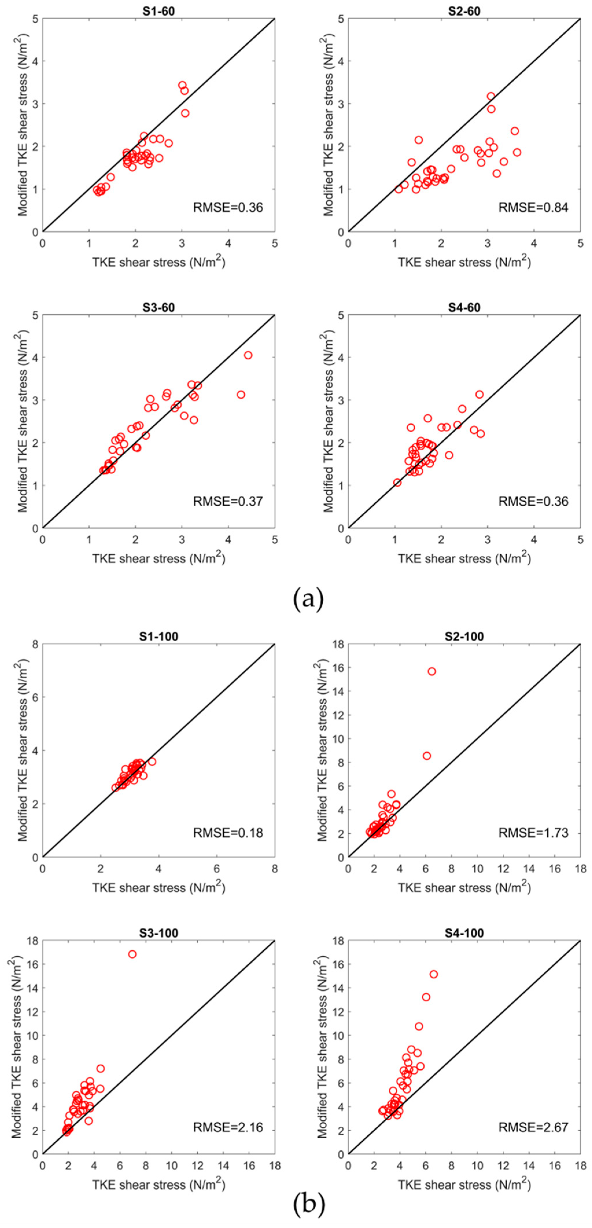
To compare the estimates of Reynolds, TKE, and modified TKE methods in a more compelling way, the near-bed shear stresses from each method for all the points were plotted against each other. Figure 4 shows the near-bed shear stress estimated using the TKE and modified TKE methods for all scenarios. Here, the goal was to understand the similarity between the near-bed shear stress estimated from the point-methods. Therefore, the root mean square error (RMSE) was selected to shed light on the similarity of the results calculated by different methods. As shown in Figure 4a, at 60 L/s scenarios, the RMSE for all the scenarios varied between 0.36 and 0.84 N/m2 indicating a reasonable similarity between results even after adding boulders and then decreasing the boulder spacing. At 100 L/s (Figure 4b), before adding boulders (S1-100), a low RMSE = 0.18 N/m2 indicated a good agreement between the TKE and modified TKE methods. After adding boulders, the RMSE significantly increased, and this increase was intensified after decreasing the boulder spacing. Generally, the modified TKE method resulted in higher values of the near-bed shear stress in comparison with the TKE method for the boulder-scenarios (S2-100, S3-100, and S4-100). This difference can be related to the values of and constants that still are required to be found for the natural streams [11,12].
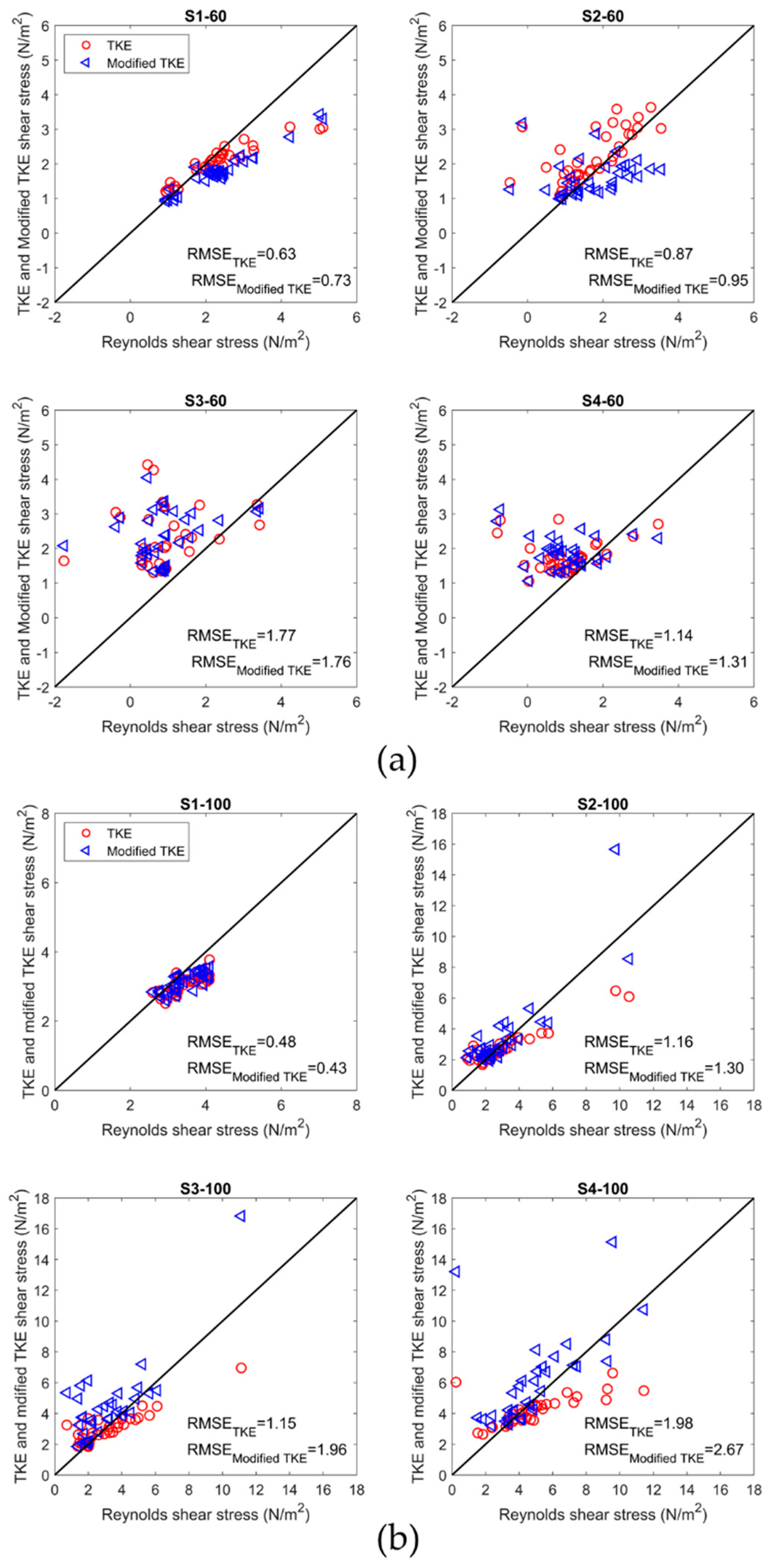
Figure 5 shows plots for comparing estimations using the Reynolds shear stress method versus the TKE and modified TKE methods. At 60 L/s and 100 L/s, before adding boulders (S1-60 and S1-100), both TKE and modified TKE methods showed a reasonable agreement with the Reynolds method (At 60 L/s, RMSE = 0.63 and 0.73 N/m2 for the TKE and modified TKE, respectively. At 100 L/s, RMSE = 0.48 and 0.43 N/m2 for the TKE and modified TKE, respectively). It was reported that the modified TKE and Reynolds method have a relatively good agreement over a Plexiglas and sand bed [12]. However, estimations using the TKE and modified TKE methods were mostly lower than the Reynolds method, but at a lower range of shear stresses, the values were close to 1:1 line. This behavior in a range of high shear stress is in agreement with [12]; however, for the lower shear stresses, similar studies found systematically higher values from the TKE and modified TKE methods [12,40]. For the large boulder spacing at 60 L/s (S2-60), the agreement between the Reynolds and both TKE and modified TKE methods slightly decreased (RMSE = 0.87 and 0.95 N/m2 for the TKE and modified TKE, respectively). By decreasing boulder spacing (S3-60 and S4-60), the RMSE increased to higher values indicating a lower similarity between the methods. A reason for the poor performance can be the presence of negative values in the Reynolds method, while values using two other methods are always positive. After adding boulders, it can be found that both TKE and modified TKE methods led to higher estimations than the Reynolds method (except for the modified TKE method at the large boulder spacing). This difference became more significant for the medium and small boulder spacing scenarios. At 100 L/s for the boulder-scenarios, the RMSE of the Reynolds and TKE methods varied between 1.16 and 1.98 N/m2, and the RMSE of the Reynolds and modified TKE methods varied between 1.30 to 2.67 N/m2. The RMSE values for both TKE and modified TKE methods reached their maximum (lower similarity) for the small boulder spacing (S4-100). However, some extreme values resulted from the TKE and modified TKE methods might be the reason behind higher RMSE values. After adding boulders, the TKE method estimates generally were smaller than the Reynolds method, while the modified TKE method usually resulted in higher near-bed shear stress than the Reynolds method.
3.3. Spatial Distribution of Near-Bed Shear Stress
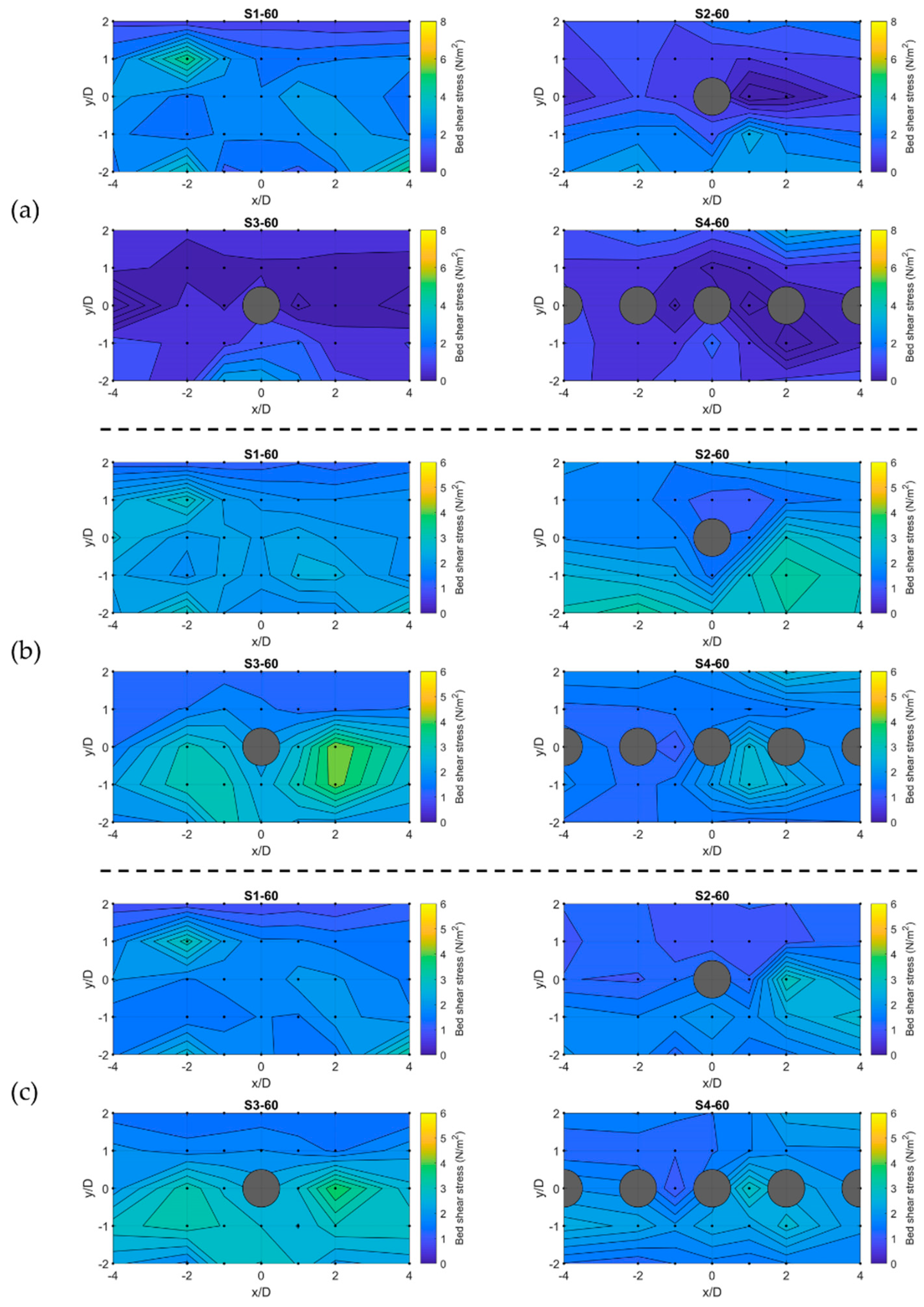
The spatial distribution of the near-bed shear stress is also of great importance, especially in the presence of boulders that significantly alter local flow fields. On this account, contour maps of estimated local near-bed shear stress using different methods were plotted. Figure 6 shows contour plots of the estimated near-bed shear stress using the Reynolds, TKE, and modified TKE methods at unsubmerged condition (60 L/s). Before adding boulders (S1-60) for all methods, a uniform spatial distribution of the near-bed shear stress was expected. However, as shown in Figure 6, slightly higher near-bed shear stresses can be seen on the left side of the measurement zone before adding boulders. This non-uniform distribution can be attributed to the presence of microforms, placed slightly higher than the mean bed level, on some points of the gravel bed in these series of experiments. For the Reynolds method, after adding boulders, it can be observed that the near-bed shear stress generally decreased in all measurement points. For the large spacing scenario (S2-60), a zone with a highly decreased near-bed shear stress can be observed extended to a distance of 2D downstream of the boulder. For the medium and large boulder spacing scenarios (S3-60 and S4-60), highly decreased shear stresses can be observed along the boulder centerline and extended to the sides of the boulder. It is known that the presence of an unsubmerged boulder within the flow generates intense reverse and irregular flow in the extended wake region [30]. Here, negative shear stresses downstream of the boulder can be attributed to this reverse flow [60]. Additionally, at the smaller boulder spacing with a wake-interference or skimming flow regime, the flow deceleration becomes more pronounced between the boulder [38]. This can be the reason for the low shear stress zone along the boulder centerline for scenarios with a smaller boulder spacing (S3-60 and S4-60) [38]. The spatial distribution of the near-bed shear stress using the TKE and modified TKE methods were similar to each other. The reason for this similarity can be a less significant streamwise velocity due to the reverse flow that led to a more important role of in the calculation of shear stress using the TKE and modified TKE shear stress. Therefore, in this condition, the behavior of the TKE method became more similar to the modified TKE method that only depends on . However, the TKE and modified TKE spatial distribution deviated from the Reynolds method. In contrast to the Reynolds method, there was a slight increase in the near bed-bed shear stress downstream of the boulders (except downstream of one of the boulders in the S4-60). This increase became more significant for the medium boulder spacing. On the sides of the boulder, the near-bed shear stress did not vary significantly in comparison with the no-boulder scenario.
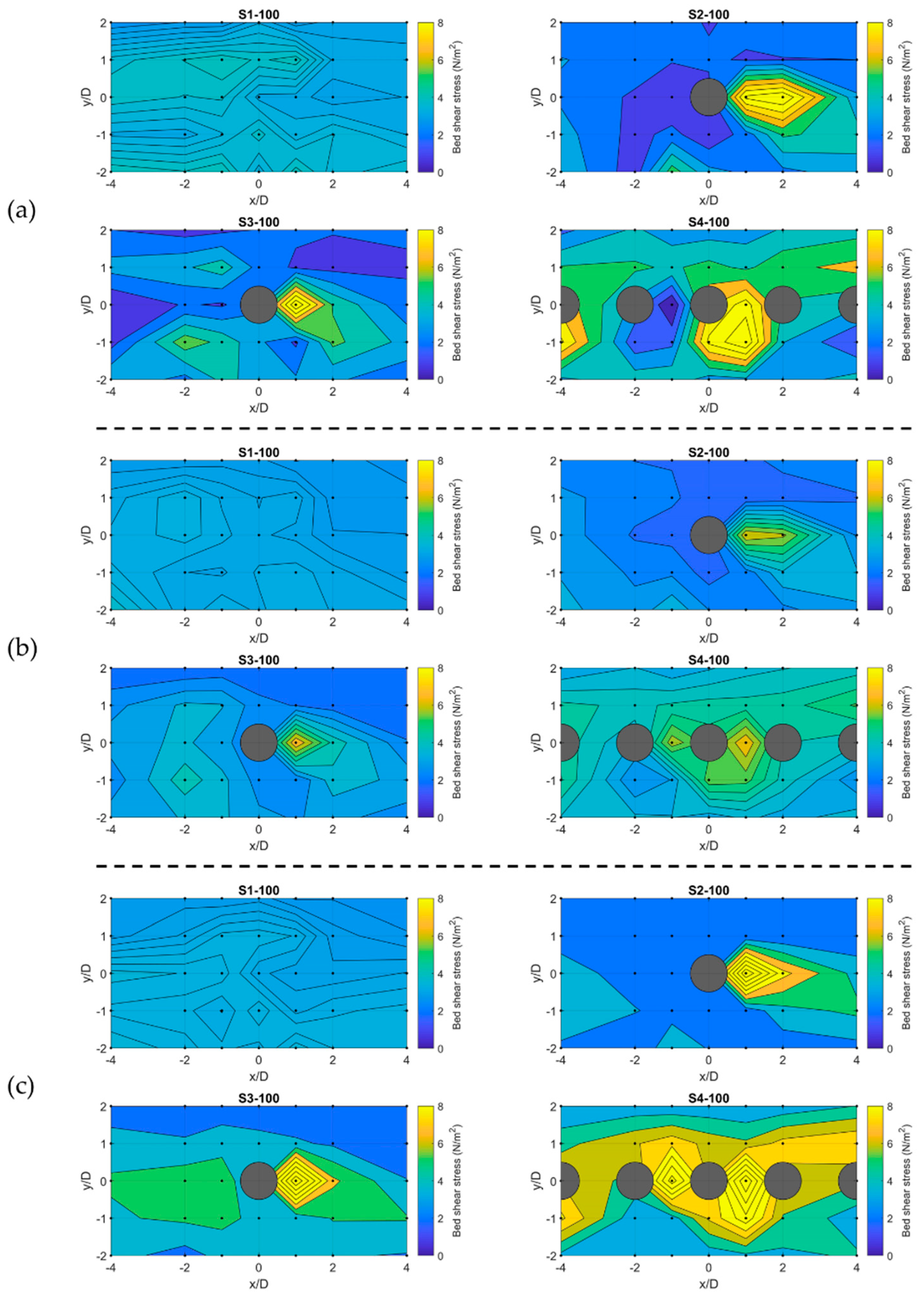
At 100 L/s (Figure 7), the spatial distribution of the near-bed shear stress using the point-methods was similar to each other, but it was different from 60 L/s. In the large boulder spacing scenario (S2-100), the near-bed shear stress decreased upstream of the boulder, but a significant increase can be seen downstream of the boulder (extended to around 2D) for all the methods. Studies have reported an increased Reynolds shear stress and TKE downstream of a submerged boulder near the bed due to the large-scale vortices in the wake zone and the presence of vertical eddies due to the downwash flow [21,31,61,62]. This increased near-bed shear stress decreased with increasing downstream x/D distance. Similarly, it has been reported this high shear stress zone extended up to the reattachment point, and then the shear stress started to decrease as undisturbed turbulent intensities recovered [31,62]. For the medium boulder spacing scenarios (S3-100), again an increased shear stress zone can be observed downstream of the central boulder for all the methods; however, for the Reynolds method a decrease in the near-bed shear stress observed at X1Y3 at x/D = −4D, downstream of one of the boulders (this boulder has not been shown in the contour plot). Additionally, the length of the high shear stress zone decreased to approximately 1D. Upstream of the boulder, the near-bed shear stress using the Reynolds method decreased, while increased shear stress can be seen upstream of the boulders for the TKE and modified TKE methods. For the small boulder spacing (S4-100), high shear stress zones became more pronounced in the sides of the boulder in this scenario. Increased near-bed shear stresses can also be seen between boulders probably as a result of the stable vortices between boulders in a wake-interference or skimming flow regime [63]. However, for the Reynolds method, a decreased shear stress zone was observed upstream of the central boulder (X3Y3 at x/D = −1D). The reason for this alternate variation of the Reynolds method estimations between boulders for the medium and small boulder spacing remained unclear and required additional experiments. For all scenarios at 100 L/s, it can be seen that the modified TKE method resulted in a higher magnitude of near-bed shear stress, as already shown in Figure 3b. The main reason for this can be attributed to the uncertain values of and , as mentioned earlier.
3.4. Near-Bed Turbulent Events
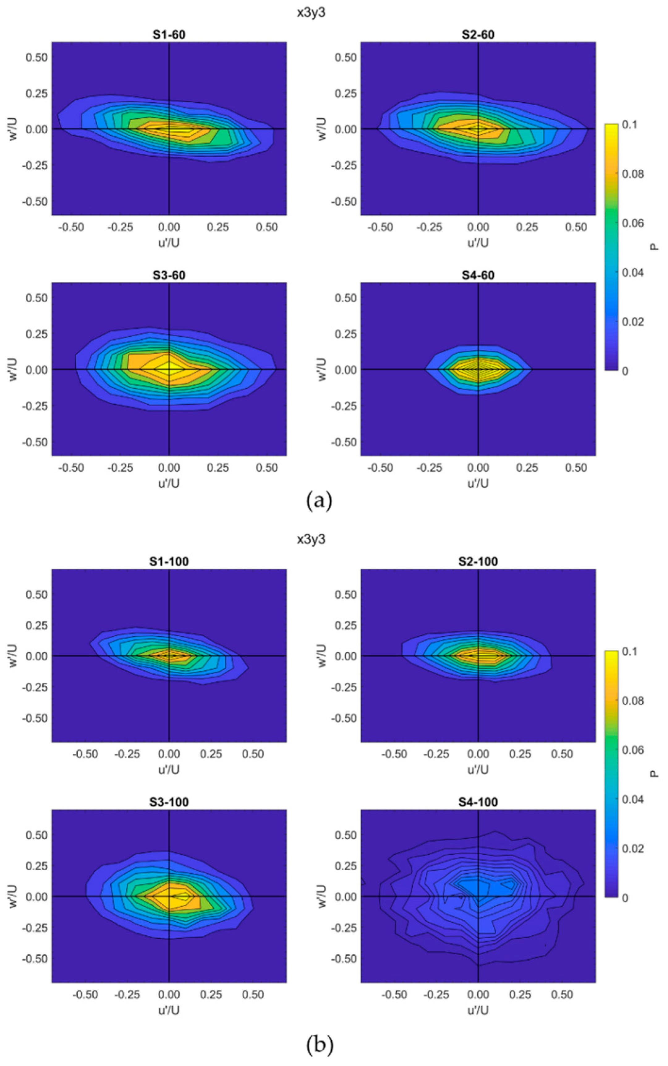
Quadrant analysis was conducted for the common points in all scenarios, X3Y3 and X5Y3. Figure 8 and Figure 9 show the joint frequency distribution of normalized and at X3Y3 and X5Y3, respectively. and were normalized by the reach-averaged velocity of each scenario. Table 2 and Table 3 complement the results of the quadrant analysis by listing the stress fraction parameter () and the frequency parameter () for each quadrant at X3Y3 and X5Y3, respectively. Before adding boulders at both points and flow rates, as expected ejection and sweep events were dominant near the bed, and this was in agreement with the previous studies [41,64]. At both flow rates at X3Y3, after adding and then decreasing the boulder spacing, the shear stress fraction of ejections and sweeps increased while the frequency of them gradually decreased. However, sweeps and ejections remained dominant for the large and medium boulder spacing. As can be seen in Figure 8 and Table 2, for the small boulder spacing, all four quadrants showed almost an equal contribution to the Reynolds shear stress and frequency. This is in agreement with the findings of [38] in which they found ejections and sweeps dominant for 10D and 5D spacing, while for 2D spacing each quadrant showed an almost equal frequency upstream of a fully submerged boulder [38]. This can be attributed to the stable vortices and a less pronounced downwash flow at the wake-interference or skimming flow associated with the small boulder spacing.
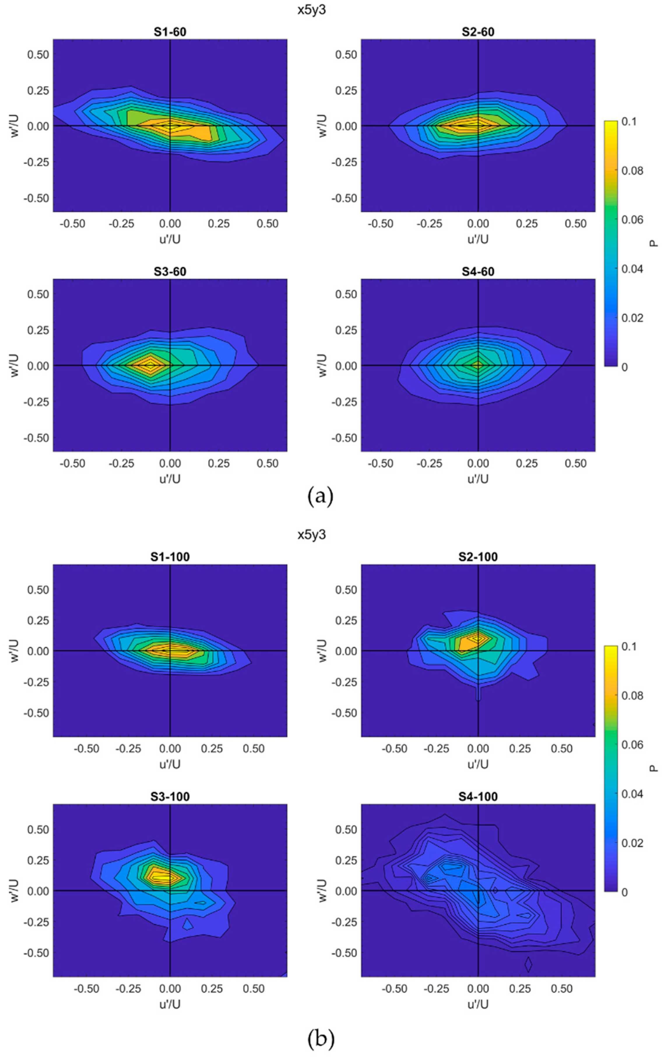
At 60 L/s at X5Y3 (Figure 9a), for the large boulder spacing (S2-60), inward and outward interactions were dominant. At the medium boulder spacing (S3-60), outward interactions and sweep events showed higher and . Again, at the small boulder spacing (S4-60), outward and inward interactions became dominant. Although 60 L/s indicates an unsubmerged boulder condition, the pattern of changes in the turbulent events was completely in agreement with the results of [38] for the different spacing of a fully submerged boulder. At 100 L/s at X5Y3 (Figure 9b), ejection and sweep events remained dominant in all scenarios while the share of inward and outward interactions was very small. However, as shown in Table 3, between ejection and sweep events, sweeps showed significantly higher and . This was not in agreement with the findings of [38] specifically for 5D and 2D boulder spacing [38]. Besides, and showed a consistent trend that means kept the same order of dominance of (e.g., when for ejections and sweeps was the highest, was also the highest for ejections and sweeps). The turbulent events have a considerable effect on sediment transport and resuspension. Predominant burst events (ejections and sweeps) may affect the sediment resuspension and transport around the boulder [39,40,41]. Specifically, downstream of the boulder, sweeps may remain effective for the bedload transport at the medium and large boulder spacing, while less significant ejections may decrease the sediment entrainment and the fine sediment suspension in these zones. Additionally, adding boulders and reduction of ejection and sweep events may provide resting zones and a path to avoid high ejection zones for the fish [43]. Such areas can be found downstream of the boulders at the medium and large boulder spacing where the burst events reduced in comparison with the no-boulder condition. However, more investigation is necessary to find the role of turbulent events in sediment transport and habitat preference for different boulder spacing.
4. Conclusions
This study investigated the effects of boulder spacing and boulder submergence ratio on the near-bed shear stress estimations and their distributions using laboratory experiments. The following conclusions can be drawn from this study:
- For all scenarios, the reach-averaged method led to a significantly higher reach-averaged bed shear stress. For the unsubmerged condition, the Reynolds method resulted in a significantly lower near-bed shear stress between the point-methods, while, at submerged condition, all the point-methods showed very similar results.
- At unsubmerged condition, the effect of the boulder spacing on the variation of near-bed shear stress estimated from the Reynolds method was different from the TKE and modified TKE methods, while, at submerged condition, all of the point-methods showed a similar trend.
- At submerged condition, the densest boulder spacing led to the highest near-bed shear stress for all point-methods. However, for the unsubmerged condition, maximum near-bed shear stress varied for different methods and boulder spacing.
- At unsubmerged condition, the TKE and modified TKE methods can be used interchangeably for estimation of the near-bed shear stress in the presence of boulders; however, applying appropriate and coefficients is required to obtain more reliable results. For a comprehensive comparison of the Reynolds method with two other point-methods, more measurements are necessary, especially at unsubmerged condition.
- At unsubmerged condition, denser boulder spacing led to a more uniform contribution of turbulent events to the Reynolds shear stress. At submerged condition, decreased ejection events downstream of boulders in the large and medium boulder spacing may reduce the sediment entrainment and suspension.
This work is based on two boulder submergence ratios and single-point measurements near the bed and placing boulders along the centerline of the channel in a single straight array. To derive general conclusions, further measurements closer to the bed with a denser spatial grid between boulders are necessary. Additionally, a study of the bedload and the suspended load sediment transport within different boulder setups is recommended as the next step.
Author Contributions
Conceptualization, A.B.M.B.; methodology, A.G.; software, A.G.; formal analysis, A.G.; investigation, A.G. and F.H.; resources, A.B.M.B.; data curation, A.G. and F.H.; writing—original draft preparation, A.G. and F.H.; writing—review and editing, A.B.M.B., F.H. and A.G.; visualization, A.G.; supervision, A.B.M.B.; project administration, A.B.M.B.; All authors have read and agreed to the published version of the manuscript.
Funding
This research received no external funding. However, financial support for the first author was provided by Clarkson University.
Acknowledgments
The authors wish to thank Ian Knack (Clarkson University) for his invaluable support and help to build the Ecohydraulics Flume.
Conflicts of Interest
The authors declare no conflict of interest.
References
- Barnes, M.P.; O’donoghue, T.; Alsina, J.M.; Baldock, T.E. Direct bed shear stress measurements in bore-driven swash. Coast. Eng. 2009, 56, 853–867. [Google Scholar] [CrossRef] [Green Version]
- Howe, D.; Blenkinsopp, C.E.; Turner, I.L.; Baldock, T.E.; Puleo, J.A. Direct measurements of bed shear stress under swash flows on steep laboratory slopes at medium to prototype scales. J. Mar. Sci. Eng. 2019, 7, 358. [Google Scholar] [CrossRef] [Green Version]
- Mirfenderesk, H.; Young, I.R. Direct measurements of the bottom friction factor beneath surface gravity waves. Appl. Ocean Res. 2003, 25, 269–287. [Google Scholar] [CrossRef]
- Park, J.H.; Do Kim, Y.; Park, Y.S.; Jo, J.A.; Kang, K. Direct measurement of bottom shear stress under high-velocity flow conditions. Flow Meas. Instrum. 2016, 50, 121–127. [Google Scholar] [CrossRef]
- Park, J.H.; Do Kim, Y.; Park, Y.S.; Jung, D.G. Direct measurement of bed shear stress using adjustable shear plate over a wide range of Froude numbers. Flow Meas. Instrum. 2019, 65, 122–127. [Google Scholar] [CrossRef]
- Nezu, I.; Nakagawa, H. Turbulence in Open Channel Flows, IAHR; Balkema: Rotterdam, The Netherlands, 1993. [Google Scholar]
- Babaeyan-Koopaei, K.; Ervine, D.A.; Carling, P.A.; Cao, Z. Velocity and turbulence measurements for two overbank flow events in River Severn. J. Hydraul. Eng. 2002, 128, 891–900. [Google Scholar] [CrossRef]
- Wilcock, P.R. Estimating local bed shear stress from velocity observations. Water Resour. Res. 1996, 32, 3361–3366. [Google Scholar] [CrossRef]
- Williams, J.J. Drag and sediment dispersion over sand waves. Estuar. Coast. Shelf Sci. 1995, 41, 659–687. [Google Scholar] [CrossRef]
- Nikora, V.; Goring, D.; McEwan, I.; Griffiths, G. Spatially averaged open-channel flow over rough bed. J. Hydraul. Eng. 2001, 127, 123–133. [Google Scholar] [CrossRef]
- Kim, S.-C.; Friedrichs, C.T.; Maa, J.-Y.; Wright, L.D. Estimating bottom stress in tidal boundary layer from acoustic Doppler velocimeter data. J. Hydraul. Eng. 2000, 126, 399–406. [Google Scholar] [CrossRef] [Green Version]
- Biron, P.M.; Robson, C.; Lapointe, M.F.; Gaskin, S.J. Comparing different methods of bed shear stress estimates in simple and complex flow fields. Earth Surf. Process. Landf. J. Br. Geomorphol. Res. Group 2004, 29, 1403–1415. [Google Scholar] [CrossRef]
- Lichtneger, P.; Sindelar, C.; Schobesberger, J.; Hauer, C.; Habersack, H. Experimental investigation on local shear stress and turbulence intensities over a rough non-uniform bed with and without sediment using 2D particle image velocimetry. Int. J. Sediment Res. 2020, 35, 193–202. [Google Scholar] [CrossRef]
- Kostaschuk, R.; Villard, P.; Best, J. Measuring velocity and shear stress over dunes with acoustic Doppler profiler. J. Hydraul. Eng. 2004, 130, 932–936. [Google Scholar] [CrossRef]
- Sime, L.C.; Ferguson, R.I.; Church, M. Estimating shear stress from moving boat acoustic Doppler velocity measurements in a large gravel bed river. Water Resour. Res. 2007, 43. [Google Scholar] [CrossRef] [Green Version]
- Federal Interagency Stream Restoration Working Group (15 US Federal Agencies). Stream Corridor Restoration: Principles, Processes, and Practices; GPO Item No. 0120-A; FISRWG: Washington, DC, USA, 1998. [Google Scholar]
- Kang, S.; Hill, C.; Sotiropoulos, F. On the turbulent flow structure around an instream structure with realistic geometry. Water Resour. Res. 2016, 52, 7869–7891. [Google Scholar] [CrossRef]
- Marttila, H.; Turunen, J.; Aroviita, J.; Tammela, S.; Luhta, P.-L.; Muotka, T.; Kløve, B. Restoration increases transient storages in boreal headwater streams. River Res. Appl. 2018, 34, 1278–1285. [Google Scholar] [CrossRef]
- Henry, C.P.; Amoros, C.; Roset, N. Restoration ecology of riverine wetlands: A 5-year post-operation survey on the Rhone River, France. Ecol. Eng. 2002, 18, 543–554. [Google Scholar] [CrossRef]
- Baki, A.B.M.; Zhu, D.Z.; Rajaratnam, N. Mean flow characteristics in a rock-ramp-type fish pass. J. Hydraul. Eng. 2014, 140, 156–168. [Google Scholar] [CrossRef]
- Baki, A.B.M.; Zhu, D.Z.; Rajaratnam, N. Turbulence characteristics in a rock-ramp-type fish pass. J. Hydraul. Eng. 2015, 141, 04014075. [Google Scholar] [CrossRef]
- Baki, A.B.M.; Zhang, W.; Zhu, D.Z.; Rajaratnam, N. Flow structures in the vicinity of a submerged boulder within a boulder array. J. Hydraul. Eng. 2016, 143, 04016104. [Google Scholar] [CrossRef]
- Papanicolaou, A.N.; Tsakiris, A.G. Boulder effects on turbulence and bedload transport. In Gravel-Bed Rivers; John Wiley & Sons, Ltd: Hoboken, NJ, USA, 2017; pp. 33–72. [Google Scholar]
- Tsakiris, A.G.; Papanicolaou, A.N.T.; Hajimirzaie, S.M.; Buchholz, J.H.J. Influence of collective boulder array on the surrounding time-averaged and turbulent flow fields. J. Mt. Sci. 2014, 11, 1420–1428. [Google Scholar] [CrossRef]
- Papanicolaou, A.N.; Dermisis, D.C.; Elhakeem, M. Investigating the role of clasts on the movement of sand in gravel bed rivers. J. Hydraul. Eng. 2011, 137, 871–883. [Google Scholar] [CrossRef]
- Hardy, R.J.; Best, J.L.; Lane, S.N.; Carbonneau, P.E. Coherent flow structures in a depth-limited flow over a gravel surface: The role of near-bed turbulence and influence of Reynolds number. J. Geophys. Res. Earth Surf. 2009, 114. [Google Scholar] [CrossRef] [Green Version]
- Van Rijn, L.C. Critical movement of large rocks in currents and waves. Int. J. Sediment Res. 2019, 34, 387–398. [Google Scholar] [CrossRef]
- Papanicolaou, A.N.; Kramer, C.M.; Tsakiris, A.G.; Stoesser, T.; Bomminayuni, S.; Chen, Z. Effects of a fully submerged boulder within a boulder array on the mean and turbulent flow fields: Implications to bedload transport. Acta Geophys. 2012, 60, 1502–1546. [Google Scholar] [CrossRef]
- Yager, E.M.; Kirchner, J.W.; Dietrich, W.E. Calculating bed load transport in steep boulder bed channels. Water Resour. Res. 2007, 43. [Google Scholar] [CrossRef]
- Shamloo, H.; Rajaratnam, N.; Katopodis, C. Hydraulics of simple habitat structures. J. Hydraul. Res. 2001, 39, 351–366. [Google Scholar] [CrossRef]
- Dey, S.; Sarkar, S.; Bose, S.K.; Tait, S.; Castro-Orgaz, O. Wall-wake flows downstream of a sphere placed on a plane rough wall. J. Hydraul. Eng. 2011, 137, 1173–1189. [Google Scholar] [CrossRef]
- Monsalve, A.; Yager, E.M. Bed surface adjustments to spatially variable flow in low relative submergence regimes. Water Resour. Res. 2017, 53, 9350–9367. [Google Scholar] [CrossRef]
- Ghilardi, T.; Schleiss, A. Influence of immobile boulders on bedload transport in a steep flume. In Proceedings of the 34th IAHR World Congress, Brisbane, Australia, 26 June–1 July 2011; pp. 3473–3480. [Google Scholar]
- Ghilardi, T.; Schleiss, A. Steep flume experiments with large immobile boulders and wide grain size distribution as encountered in alpine torrents. In Proceedings of the International conference on fluvial Hydraulics, San José, Costa Rica, 5–7 September 2012; Taylor & Francis Group, CRC Press: London, UK, 2012; pp. 407–414. [Google Scholar]
- Papanicolaou, A.N.; Tsakiris, A.G.; Wyssmann, M.A.; Kramer, C.M. Boulder Array Effects on Bedload Pulses and Depositional Patches. J. Geophys. Res. Earth Surf. 2018, 123, 2925–2953. [Google Scholar] [CrossRef]
- Papanicolaou, A.N.; Diplas, P.; Dancey, C.L.; Balakrishnan, M. Surface Roughness Effects in Near-Bed Turbulence: Implications to Sediment Entrainment. J. Eng. Mech. 2001, 127, 211–218. [Google Scholar] [CrossRef]
- Shih, W.; Diplas, P.; Celik, A.O.; Dancey, C. Accounting for the role of turbulent flow on particle dislodgement via a coupled quadrant analysis of velocity and pressure sequences. Adv. Water Resour. 2017, 101, 37–48. [Google Scholar] [CrossRef] [Green Version]
- Fang, H.W.; Liu, Y.; Stoesser, T. Influence of Boulder Concentration on Turbulence and Sediment Transport in Open-Channel Flow Over Submerged Boulders. J. Geophys. Res. Earth Surf. 2017, 122, 2392–2410. [Google Scholar] [CrossRef]
- Tang, C.; Li, Y.; Acharya, K.; Du, W.; Gao, X.; Luo, L.; Yu, Z. Impact of intermittent turbulent bursts on sediment resuspension and internal nutrient release in Lake Taihu, China. Environ. Sci. Pollut. Res. 2019, 26, 16519–16528. [Google Scholar] [CrossRef] [PubMed]
- Salim, S.; Pattiaratchi, C.; Tinoco, R.; Coco, G.; Hetzel, Y.; Wijeratne, S.; Jayaratne, R. The influence of turbulent bursting on sediment resuspension under fluvial unidirectional currents. Earth Surf. Dyn. 2016, 5, 399–415. [Google Scholar] [CrossRef] [Green Version]
- Mohajeri, S.H.; Righetti, M.; Wharton, G.; Romano, G.P. On the structure of turbulent gravel bed flow: Implications for sediment transport. Adv. Water Resour. 2016, 92, 90–104. [Google Scholar] [CrossRef]
- Lacey, R.J.; Rennie, C.D. Laboratory investigation of turbulent flow structure around a bed-mounted cube at multiple flow stages. J. Hydraul. Eng. 2012, 138, 71–84. [Google Scholar] [CrossRef]
- Bretón, F.; Baki, A.B.M.; Link, O.; Zhu, D.Z.; Rajaratnam, N. Flow in nature-like fishway and its relation to fish behaviour. Can. J. Civ. Eng. 2013, 40, 567–573. [Google Scholar] [CrossRef]
- Polatel, C. Large-Scale Roughness Effect on Free-Surface and Bulk Flow Characteristics in Open-Channel Flows. Ph.D. Thesis, University of Iowa, Iowa City, IA, USA, 2006. [Google Scholar]
- Tan, L.; Curran, J.C. Comparison of Turbulent Flows over Clusters of Varying Density. J. Hydraul. Eng. 2012, 138, 1031–1044. [Google Scholar] [CrossRef]
- Paphitis, D. Sediment movement under unidirectional flows: An assessment of empirical threshold curves. Coast. Eng. 2001, 43, 227–245. [Google Scholar] [CrossRef]
- Nezu, I.; Rodi, W. Open-channel Flow Measurements with a Laser Doppler Anemometer. J. Hydraul. Eng. 1986, 112, 335–355. [Google Scholar] [CrossRef]
- Dombroski, D.E.; Crimaldi, J.P. The accuracy of acoustic Doppler velocimetry measurements in turbulent boundary layer flows over a smooth bed. Limnol. Oceanogr. Methods 2007, 5, 23–33. [Google Scholar] [CrossRef]
- Goring, D.G.; Nikora, V.I. Despiking acoustic Doppler velocimeter data. J. Hydraul. Eng. 2002, 128, 117–126. [Google Scholar] [CrossRef] [Green Version]
- Cea, L.; Puertas, J.; Pena, L. Velocity measurements on highly turbulent free surface flow using ADV. Exp. Fluids 2007, 42, 333–348. [Google Scholar] [CrossRef]
- Wahl, T.L. Analyzing ADV data using WinADV. In Proceedings of the Joint Conference on Water Resources Engineering and Water Resources Planning and Managmenet, Minneapolis, MI, USA, 30 July-2 August 2000. [Google Scholar]
- Strom, K.B.; Papanicolaou, A.N. ADV measurements around a cluster microform in a shallow mountain stream. J. Hydraul. Eng. 2007, 133, 1379–1389. [Google Scholar] [CrossRef]
- Martin, V.; Fisher, T.S.R.; Millar, R.G.; Quick, M.C. ADV data analysis for turbulent flows: Low correlation problem. In Proceedings of the Hydraulic Measurements and Experimental Methods 2002, Estes Park, CO, USA, 28 July–1 August 2002; pp. 1–10. [Google Scholar]
- Nikora, V.I.; Goring, D.G. ADV measurements of turbulence: Can we improve their interpretation? J. Hydraul. Eng. 1998, 124, 630–634. [Google Scholar] [CrossRef]
- Lacey, R.W.J.; Roy, A.G. Fine-scale characterization of the turbulent shear layer of an instream pebble cluster. J. Hydraul. Eng. 2008, 134, 925–936. [Google Scholar] [CrossRef]
- Buffin-Bélanger, T.; Roy, A.G. Effects of a pebble cluster on the turbulent structure of a depth-limited flow in a gravel-bed river. Geomorphology 1998, 25, 249–267. [Google Scholar] [CrossRef]
- Curran, J.C.; Tan, L. The effect of cluster morphology on the turbulent flows over an armored gravel bed surface. J. Hydro-Environ. Res. 2014, 8, 129–142. [Google Scholar] [CrossRef]
- Liu, D.; Liu, X.; Fu, X.; Wang, G. Quantification of the bed load effects on turbulent open-channel flows: Les-Dem Simulation of Sediment in Turbulent Flow. J. Geophys. Res. Earth Surf. 2016, 121, 767–789. [Google Scholar] [CrossRef]
- Guan, D.; Agarwal, P.; Chiew, Y.-M. Quadrant Analysis of Turbulence in a Rectangular Cavity with Large Aspect Ratios. J. Hydraul. Eng. 2018, 144, 04018035. [Google Scholar] [CrossRef]
- Sadeque, M.A.; Rajaratnam, N.; Loewen, M.R. Flow around Cylinders in Open Channels. J. Eng. Mech. 2008, 134, 60–71. [Google Scholar] [CrossRef]
- Hajimirzaie, S.M.; Tsakiris, A.G.; Buchholz, J.H.J.; Papanicolaou, A.N. Flow characteristics around a wall-mounted spherical obstacle in a thin boundary layer. Exp. Fluids 2014, 55, 1762. [Google Scholar] [CrossRef]
- Zexing, X.; Chenling, Z.; Qiang, Y.; Xiekang, W.; Xufeng, Y. Hydrodynamics and bed morphological characteristics around a boulder in a gravel stream. Water Supply 2020, 20, 395–407. [Google Scholar] [CrossRef]
- Morris, H.M. Flow in rough conduits. Trans. ASME 1955, 120, 373–398. [Google Scholar]
- Nakagawa, H.; Nezu, I. Prediction of the contributions to the Reynolds stress from bursting events in open-channel flows. J. Fluid Mech. 1977, 80, 99–128. [Google Scholar] [CrossRef]
Figure 1.
A schematic plan view of the flume. The hatched area shows the detailed measurement zone.

Figure 2.
A schematic plan of boulder arrangement in the measurement zone (hatched area) for (a) no boulder, (b) 10D boulder spacing, (c) 5D boulder spacing, and (d) 2D boulder spacing. Cross marks show measurement points for each setup, and large circles show the position of idealized (assumed fully spherical) boulders. Two points X3Y3 and X5Y3 have been marked in (a) as common measurement points in the centerline of boulders in all scenarios.

Figure 3.
Averaged bed shear stress resulted from different calculation methods for different boulder spacing at (a) 60 L/s flow rate, (b) 100 L/s flow rate.
Figure 3.
Averaged bed shear stress resulted from different calculation methods for different boulder spacing at (a) 60 L/s flow rate, (b) 100 L/s flow rate.

Figure 4.
Near-bed shear stress estimated from the turbulent kinetic energy (TKE) method against the modified TKE method for all the measurement points at (a) 60 L/s flow rate, (b) 100 L/s flow rate. The unit of RMSE is N/m2.
Figure 4.
Near-bed shear stress estimated from the turbulent kinetic energy (TKE) method against the modified TKE method for all the measurement points at (a) 60 L/s flow rate, (b) 100 L/s flow rate. The unit of RMSE is N/m2.

Figure 5.
Near-bed shear stress estimated from the Reynolds method against the TKE and modified TKE methods for all the measurement points at (a) 60 L/s flow rate, (b) 100 L/s flow rate. The unit of RMSE is N/m2.
Figure 5.
Near-bed shear stress estimated from the Reynolds method against the TKE and modified TKE methods for all the measurement points at (a) 60 L/s flow rate, (b) 100 L/s flow rate. The unit of RMSE is N/m2.

Figure 6.
Contour plots of the estimated near-bed shear stress at 60 L/s (unsubmerged condition) for (a) the Reynolds, (b) TKE, and (c) modified TKE methods. Gray circles show the idealized boulders, and small black dots represent the measuring points.
Figure 6.
Contour plots of the estimated near-bed shear stress at 60 L/s (unsubmerged condition) for (a) the Reynolds, (b) TKE, and (c) modified TKE methods. Gray circles show the idealized boulders, and small black dots represent the measuring points.

Figure 7.
Contour plots of the estimated near-bed shear stress at 100 L/s (submerged condition) for (a) the Reynolds, (b) TKE, and (c) modified TKE methods. Gray circles show the idealized boulders, and small black dots represent the measuring points.
Figure 7.
Contour plots of the estimated near-bed shear stress at 100 L/s (submerged condition) for (a) the Reynolds, (b) TKE, and (c) modified TKE methods. Gray circles show the idealized boulders, and small black dots represent the measuring points.

Figure 8.
Joint frequency distribution of normalized and at point X3Y3 at (a) 60 L/s flow rate, (b) 100 L/s flow rate.
Figure 8.
Joint frequency distribution of normalized and at point X3Y3 at (a) 60 L/s flow rate, (b) 100 L/s flow rate.

Figure 9.
Joint frequency distribution of normalized and at point X5Y3 at (a) 60 L/s flow rate, (b) 100 L/s flow rate.
Figure 9.
Joint frequency distribution of normalized and at point X5Y3 at (a) 60 L/s flow rate, (b) 100 L/s flow rate.


Table 1.
Characteristics of the experiments.
| Scenario | Flow Rate (L/s) | Boulder Spacing | Reach-Averaged Flow Depth (m) | Submergence Ratio |
|---|---|---|---|---|
| S1-60 | 60 | Infinity | 0.082 | - |
| S2-60 | 10D | 0.092 | 0.73 | |
| S3-60 | 5D | 0.098 | 0.78 | |
| S4-60 | 2D | 0.093 | 0.74 | |
| S1-100 | 100 | Infinity | 0.151 | - |
| S2-100 | 10D | 0.157 | 1.25 | |
| S3-100 | 5D | 0.165 | 1.32 | |
| S4-100 | 2D | 0.161 | 1.29 |
Table 2.
Stress fraction and frequency of events for X3Y3 at 60 and 100 L/s flow rates.
| Parameter | P | |||||||
|---|---|---|---|---|---|---|---|---|
| Scenario | Outward | Ejection | Inward | Sweep | Outward | Ejection | Inward | Sweep |
| S1-60 | −0.05 | 0.55 | −0.04 | 0.41 | 0.03 | 0.36 | 0.03 | 0.27 |
| S2-60 | −0.29 | 0.74 | −0.26 | 0.74 | 0.12 | 0.30 | 0.10 | 0.30 |
| S3-60 | −1.50 | 2.17 | −1.50 | 1.83 | 0.21 | 0.30 | 0.21 | 0.25 |
| S4-60 | −10.10 | 12.01 | −9.77 | 8.86 | 0.25 | 0.29 | 0.24 | 0.22 |
| S1-100 | −0.07 | 0.51 | −0.06 | 0.50 | 0.04 | 0.32 | 0.04 | 0.31 |
| S2-100 | −0.74 | 1.25 | −0.64 | 1.11 | 0.18 | 0.31 | 0.16 | 0.27 |
| S3-100 | −0.51 | 1.14 | −0.58 | 0.93 | 0.14 | 0.32 | 0.16 | 0.26 |
| S4-100 | −12.17 | 12.29 | −11.62 | 12.49 | 0.25 | 0.25 | 0.24 | 0.26 |
Table 3.
Stress fraction and frequency of events for X5Y3 at 60 and 100 L/s flow rates.
| Parameter | P | |||||||
|---|---|---|---|---|---|---|---|---|
| Scenario | Outward | Ejection | Inward | Sweep | Outward | Ejection | Inward | Sweep |
| S1-60 | −0.02 | 0.45 | −0.03 | 0.38 | 0.01 | 0.33 | 0.02 | 0.28 |
| S2-60 | 1.24 | −0.57 | 1.14 | −0.84 | 0.30 | 0.14 | 0.27 | 0.20 |
| S3-60 | 4.98 | −2.92 | 3.24 | −4.30 | 0.32 | 0.19 | 0.21 | 0.28 |
| S4-60 | 1.41 | −0.90 | 1.48 | −1.00 | 0.28 | 0.18 | 0.29 | 0.20 |
| S1-100 | −0.08 | 0.59 | −0.10 | 0.49 | 0.05 | 0.34 | 0.06 | 0.28 |
| S2-100 | −0.06 | 0.22 | −0.03 | 0.72 | 0.04 | 0.15 | 0.02 | 0.49 |
| S3-100 | −0.02 | 0.23 | −0.03 | 0.62 | 0.02 | 0.17 | 0.02 | 0.45 |
| S4-100 | −0.05 | 0.39 | −0.03 | 0.49 | 0.03 | 0.27 | 0.02 | 0.34 |
© 2020 by the authors. Licensee MDPI, Basel, Switzerland. This article is an open access article distributed under the terms and conditions of the Creative Commons Attribution (CC BY) license (http://creativecommons.org/licenses/by/4.0/).
Share and Cite
MDPI and ACS Style
Golpira, A.; Huang, F.; Baki, A.B.M. The Effect of Habitat Structure Boulder Spacing on Near-Bed Shear Stress and Turbulent Events in a Gravel Bed Channel. Water 2020, 12, 1423. https://doi.org/10.3390/w12051423
AMA Style
Golpira A, Huang F, Baki ABM. The Effect of Habitat Structure Boulder Spacing on Near-Bed Shear Stress and Turbulent Events in a Gravel Bed Channel. Water. 2020; 12(5):1423. https://doi.org/10.3390/w12051423
Chicago/Turabian StyleGolpira, Amir, Fengbin Huang, and Abul B.M. Baki. 2020. "The Effect of Habitat Structure Boulder Spacing on Near-Bed Shear Stress and Turbulent Events in a Gravel Bed Channel" Water 12, no. 5: 1423. https://doi.org/10.3390/w12051423
Note that from the first issue of 2016, this journal uses article numbers instead of page numbers. See further details here.