Calibration Procedure for Water Distribution Systems: Comparison among Hydraulic Models


1
Faculty of Science and Technology, Free University of Bozen-Bolzano, Piazza Università 5, 39100 Bolzano, Italy
2
Department of Civil, Environmental and Mechanical Engineering, University of Trento, via Mesiano 77, 38123 Trento, Italy
*
Author to whom correspondence should be addressed.
Water 2020, 12(5), 1421; https://doi.org/10.3390/w12051421
Submission received: 8 April 2020
/
Revised: 6 May 2020
/
Accepted: 14 May 2020
/
Published: 16 May 2020
(This article belongs to the Section Urban Water Management)
Abstract
:Proper hydraulic simulation models, which are fundamental to analyse a water distribution system, require a calibration procedure. This paper proposes a multi-objective procedure to calibrate water demands and pipe roughness distribution in the context of an ill-posed problem, where the number of measurements is smaller than the number of variables. The proposed methodology consists of a two-steps procedure based on a genetic algorithm. Firstly, several runs of the calibrator are performed and the corresponding pressure and flow-rates values are averaged to overcome the non-uniqueness of the solutions problem. Secondly, the final calibrated model is achieved using the calibrator with the average values of the previous step as the reference condition. Therefore, the procedure enables to obtain physically based hydraulic parameters. Moreover, several hydraulic models are investigated to assess their performance on this optimisation procedure. The considered models are based either on concentrated at nodes or distributed along pipes demands approach, but also either on demand driven or pressure driven approach. Results show the reliability of the final calibrated model in the context of the ill-posed problem. Moreover, it is observed the overall better performance of the pressure driven approach with distributed demand in scarce pressure condition.
1. Introduction
Nowadays, hydraulic simulation models are widely used for analysing the behaviour of water distribution systems. Due to the high degree of uncertainty and to the lack of details of the system, reliable management may be achieved only with an accurate calibrated model.
Calibration of water distribution models is a process that adjusts network parameters, such as pipe roughness and nodal demand [1], to minimize the differences between simulation results and real measurements. In order to be reliable, a hydraulic model requires a calibration process [2] that modifies the most sensitive parameters.
A comprehensive literature review of the water distribution network (WDN) model calibration is proposed in [1], where the calibration methods are classified as generally as possible in three different categories. Firstly, iterative and trial and error procedures, where unknown parameters are updated at each iteration [2,3]. This approach has a slow convergence rate and typically can handle only small problems. Secondly, explicit methods which are based on the solution of an extended set of steady-state equations [4]. This extended set of equations is composed of initial equations plus additional ones derived from measurements available. Thirdly, implicit methods that are based on optimization techniques. These latter have to minimise one or more objective functions considering two constraints: energy and mass equation, that are implicit in the hydraulics of the problem, and the range for the chosen variables. Several different approaches have been proposed in the literature, for instance, based on a single-objective heuristic algorithm [5,6,7] or multi-objective [8,9,10]. Furthermore, the considered calibration variables have a wide range of possible parameters, such as nodal demand and pipe roughness [8], or valve status and leak parameters [9].
For example, Meirelles et al. [11] proposed a meta-model based on an artificial neural network to forecast pressure at the network nodes. Afterwards, the calibration was performed by using a Particle Swarm Optimization to estimate pipes roughness minimising the objective function written as the difference among simulated and forecasted pressure. Do et al. [12] proposed a framework to estimate near-real time demand in a WDN. A predictor-corrector methodology is applied to predict the hydraulics of a water network, and then a particle filter-based model is used to calibrate water demands. Zhou et al. [13] developed a self-adaptive system based on Kalman filter technique to develop a dual calibration of both pipe roughness and nodal water demands in a water distribution system.
The uncertainty of the results from WDN modelling is caused by many factors, which can be classified according to Hutton et al. [14] in structural, measurements and parameter uncertainty. Structural uncertainty is related to the representation of the real system, such as model aggregation or skeletonisation. Measurement uncertainty concerns the inability of measurement devices to capture the temporal and spatial variation of consumer demand and to errors related to the measure itself. Parameter uncertainty refers to the errors of the choice of variables used to model the system. Another source of uncertainty is related to the presence of leakages in the distribution network, which has been widely studied in literature [15,16,17]. According to Kang and Lansey [18], pipes roughness and water demands are the most uncertain input parameters in a hydraulic model because they are not directly measurable. Moreover, given also the general lack of information regarding the hydraulic state of the networks, the calibration problem is typically ill-posed, meaning that the number of measurements is much smaller than the variables.
Recently Do et al. [6] proposed an approach to deal with an ill-posed calibration problem by using multiple runs of a genetic algorithm model. It was found that a good solution can be achieved in spite of the non-uniqueness of the solutions, by averaging the hydraulic simulation results of the several runs. A similar approach was proposed by Letting et al. [19], which proposed an approach based on a particle swarm optimisation. Since the stochastic nature of the calibration problem both Do et al. [6] and Letting et al. [19] made multiple runs of their optimisation algorithms and used the average of the solutions as a more accurate result.
Besides the calibration procedure, also the hydraulic modelling approach plays a crucial role in the accuracy of the results. In literature, most of the works are based on the EPANET2 [20] hydraulic solver [5,6,19,21]. The numerical solver adopted in this program is based on the Todini and Pilati [22] algorithm, which proposed a direct solution of the equations of mass conservation at the nodes and energy conservation along pipes of the WDNs. A solution is guaranteed by the convexity of the system of equations [23], but since the problem is partially non-linear, a linearization is performed and achieved through Newton-Raphson gradient technique. The resulting linear system is solved with an iterative procedure to find the nodal heads and pipe flow rates. This is called Global Gradient Algorithm (GGA).
The original GGA adopts a nodal demand driven (NDD) approach. NDD means that the water demands spread along the WDN is assumed lumped at the nodes of the network, and always fully satisfied. These assumptions can lead to inaccuracy in the model, especially in cases where the network has a deficit of pressure and is skeletonised. Therefore, many authors [24,25] modified the GGA scheme to manage scarce pressure condition, by a formulation of the water demand depending on pressure. These approaches (hereafter NPD nodal pressure driven) were still developed with the water demand concentrated at the network nodes. However, models which simulate the demand as uniformly distributed along the pipes, contrary to the node-concentrated, have been proposed to properly represent the demand distribution [26,27]. These approaches (hereafter DDD distributed demand driven) preserve the energy balance. Recently, a pressure driven distributed (DPD) implementation [28] manage to solve both the demand driven approach and concentrated demand issues.
The aim of the work is twofold: to propose a methodology to calibrate water demands and pipe roughness of a WDN through an optimisation procedure in a context of lack of measurements. In addition, to assess the influence of the hydraulic modelling on the calibration procedure, by comparing the results obtained using four different hydraulic modelling approaches. In order to achieve this aim, a static condition is considered, that is the calibration process of the roughness and water demand distribution considering a set of known flow rate at (some) pipes and pressure at (some) nodes values as measured at a given moment. In other words, the optimisation process does not consider the hourly variation of demand flow and also of heads at the tanks through an Extended Period Simulation (EPS, see [29,30]) because it is beyond the scope of the work.
In this paper, the authors propose a two-step multi-objective procedure to calibrate water demands and pipe roughness distribution. The purpose of the work is not to solve the ill-posed problem but to propose a suitable solution among all possible, that can be a solid starting point to manage a network in the condition of scarce measurements. In the first part, 100 runs of the non-dominated sorting genetic algorithm II (NSGA-II) [31] calibrator are performed in order to collect a set of pressure values at the nodes and flow rate values along the pipes. Then, with the aim to overcome the non-uniqueness of the solutions problem, average distribution of pipes flow rate and nodes pressure has been calculated by averaging the corresponding values of the 100 runs.
In the second part, the final calibration of the WDN is performed considering as the new reference condition the average values of the set of pressures and flow rate values obtained at the previous step. Therefore, in this last run, the number of variables (i.e., water demand and pipe roughness) and the number of equations is the same. The hydraulic consistency of the final solution is guaranteed by the use of optimisation with appropriate fixed boundaries, thus avoiding the problem of possible non-physical results deriving from the direct solution of the deterministic problem. This last step allows to obtain a model physically based on a set of pipe roughness and water demands. To verify the proposed approach and to accurately reproduce a real-world scenario, a reference condition is built with the spatial distribution of the withdrawals in order to represent a realistic distribution of pipes connection. Moreover, the calibration procedure is carried out with a scarce amount of measurements.
The proposed calibration procedure is tested by means of different water distribution modelling approaches, which are based either on concentrated or distributed demands, but also either on demand driven or pressure driven demand approaches. Specifically, a sequence of models is used: (1) NDD, (2) NPD, (3) DDD and (4) DPD. These approaches are implemented on the GGA to perform the simulation for the comparison in the calibration processes.
2. Methodology
The calibration of WDNs is formulated as an optimisation problem using NSGA-II. The algorithm is chosen due to its ability to effectively solve non-linear and complex optimisation engineering problems. The variables for the decisional process of the genetic algorithm are pipes roughness and average daily demand. The parameters of the algorithm are selected to ensure the stability of the solutions: this is achieved after multiple runs of the calibration process, and it is decided to use 25% probability to perform a polynomial mutation and 90% probability to perform a simulated binary crossover.
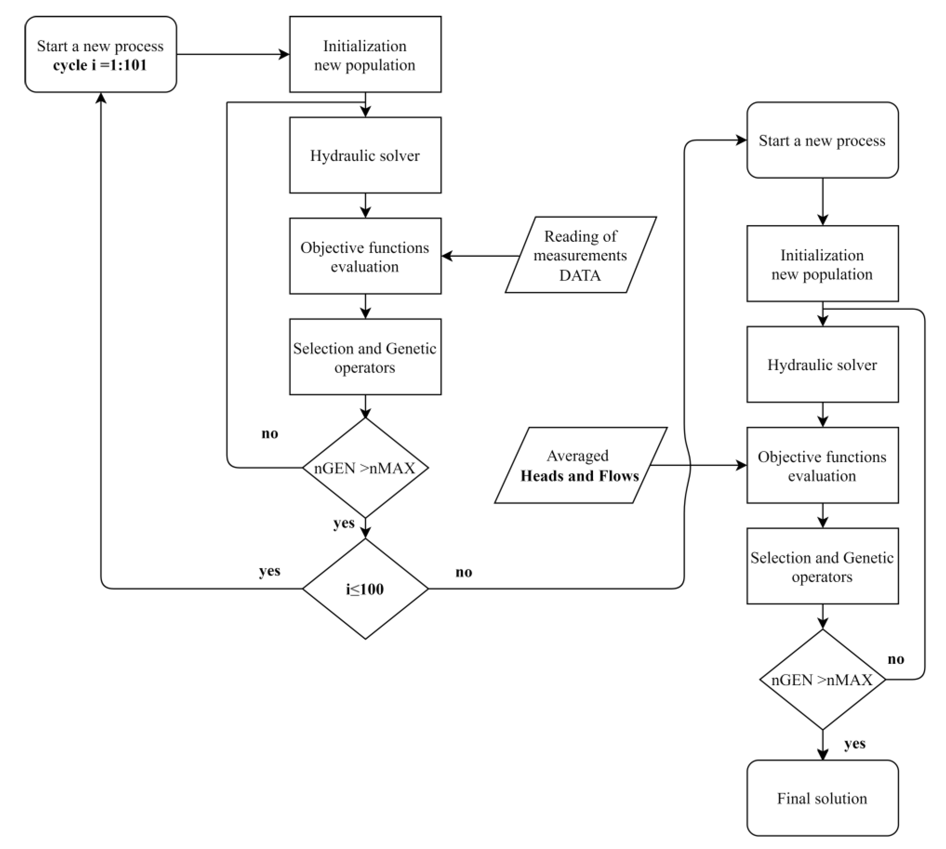
Figure 1 shows the flowchart of the proposed methodology characterised by two steps. Due to the stochastic nature of the optimisation procedure, the problem does not have a unique solution [19]. In the first part of the methodology, 100 runs of the algorithm are performed as proposed in [6]. For every cycle of the multi-objective genetic algorithm, firstly the initialisation of a random population with the shuffle of the random seed is performed. Then, the initialisation variables are used as input for the hydraulic model, which returns the nodal hydraulic heads and the pipe flow rates for each chromosome.
Afterwards, the two objective functions, which are expressed as the difference among measured and simulated values of pressure at the nodes and flow rate along the pipes, are evaluated. The selection process starts with the non-dominated sorting criteria based on the tournament selection procedure. The population, divided in half from the previous step, has to encounter the two genetic operators. These latter are the simulated binary crossover, whose aim is to combine the variables between different chromosomes, and the polynomial mutation that has to guarantee the variability with random addition. As a result, a new generation is created, and a new iteration starts. In this first part, it is adopted 300 for population number and 500 for generation number in the genetic algorithm procedure.
After 100 runs, the solutions that minimise the Euclidean distance with the best point, which in this case is the origin of the Euclidean space, are selected for each run. Then, the hydraulic output of every selected solution is collected in order to have a set of 100 pressure values for each node and 100 flow rate values for each pipe. Therefore, both sets of pressure and flow rate are averaged to result in a single solution. These average values are a good estimation of the reference condition [6,19], but they are not directly reproducible through a hydraulic simulation. It means that they do not correspond to a set of roughness and a set of water demands. To overcome this problem, the authors propose a second step where the WDN is calibrated with another run of the NSGA-II, using the objective function written as the difference among averaged and simulated pressure at the nodes and flow rates along the pipes. Thus, the number of equations and the number of variables is the same. The population and generation numbers of this second step are 300 and 1000, respectively and the selection criteria is equal to the first step. This process is carried out for the four different hydraulic approaches proposed.
2.1. Non-Uniqueness of the Solutions
The optimisation problem has a stochastic nature due to the lack of detailed information that affects most of the WDNs. In particular, the uncertainty on the values of the parameters of the network (e.g., water demands and pipes roughness) generates differences between models and real WDN. To overcome this problem, it is necessary to use measurements taken from the real network to calibrate the model. However, it is impossible for practical and economic reasons, to have a pressure measurement for each node and a flow rate measurement for each pipe. The solutions obtained for each run of the calibration procedure through the optimisation algorithm, represent a set of possible solutions. This is given by the fact that a single solution of a run might represent the process of convergence of the optimisation procedure to a local minimum that can be far from the best solution.
In order to overcome this problem, the approach used is similar to the one proposed in [6] and 100 runs are performed and used to develop the procedure. Despite the lack of information, it was shown that a good solution could be found by using the average of the 100 solutions.
However, the average pressure and flow rate values are not reproducible through a hydraulic simulation due to the unknown corresponding pipes roughness and water demands. To solve this limit, the last step is performed using as measurements data the average values of the 100 runs. Since the average pressure in each node and the average flow rates in each pipe is known, the number of equations and the number of variables is the same. The solution that is achieved is finally composed with the set of roughness and water demands that allow to reproduce the average values.
2.2. Hydraulic Models
The traditional modelling of WDNs concerns a system of energy and mass balances to provide the nodal hydraulic heads and pipe flow rates.
The NDD approach involves water demand aggregated at the network nodes, which is fully satisfied [32,33] independent from pressure condition, leading to the following mass balance equation at nodes:
where and are the top pipe node and the end pipe node, respectively. is the pipe flow rate, and is the nodal water demand. The corresponding energy balance equation of the pipe reads as:
where represents the pipe length, represents a coefficient that depends on the head loss mathematical formulation and is the nodal hydraulic head. The Darcy-Weisbach expression with equal to 2 is used in this work. This approach has become the standard for WDN hydraulic models.
For a proper simulation in scarce pressure condition, the NPD approach has been proposed [34,35,36,37]. In particular, real water demands depend on the available hydraulic pressure at the nodes. Thus, the mass balance equation at nodes results:
The energy balance equation remains Equation (2) because the flow rate along the pipe is still a constant value.
However, this approach considers water demands as aggregated at the network nodes even though the real withdrawals are distributed along the network pipes [38]. Some authors [26,27,39] have integrated a uniformly distributed demand along pipe into GGA scheme but maintaining the water demand independent from pressure. This new demand representation leads to a linear flow rate variation along pipe. In this case, the mass balance at nodes can be computed as:
where represents the water demand uniformly distributed along the pipes. The corresponding energy balance equation in the pipe reads as:
Recently, a model that combines both distributed demand and pressure driven approach has been proposed [28]. Without pressure deficit, the DPD can be simplified to the mathematical formulation of the DDD, i.e., with water demand uniformly distributed and independent from pressure. However, in case of pressure deficit condition, the DPD approach is able to solve pressure driven simulation with uniformly distributed water demand. In order to do that, the actual water demand function is approximated with a second order polynomial function as:
where represents the water demand function along the pipe with spatial coordinate and , and are three coefficients dependent from the pressure in the pipe. For additional details see Appendix A in [28]. The mass balance at nodes can be read as:
Hence, the energy balance equation over the pipe is directly integrable, and can be read as:
in case of a second-order polynomial water demand function, the complete integrated expression can be found in [28]. Summarising, the hydraulic approaches adopted in this paper concern the NDD based on Equations (1) and (2), the NPD based on Equations (2) and (3), the DDD based on Equations (4) and (5) and the DPD based on Equations (7) and (8).
In the four methodologies, the Darcy-Weisbach equation is used to model the energy losses. In both NPD and DPD models the used pressure demand relationship at node is:
where represents the water requested at node, is the pressure at node and and are coefficient defined as [25,34] and can be read as:
In Equation (10) represent the minimum hydraulic pressure condition where the outflow is zero (in our case it is fixed to 0) and is the hydraulic pressure where the water request is fully satisfied (fixed to 30 m).
2.3. Decision Variables
The variables involved in the calibration process are the pipe roughness and the water demand. Since only poor information regard pipes roughness is typically available for a real WDN, a wide variable range between 0.1 mm and 1 mm is selected. The chosen range is intended to cover the possible roughness values for a common steel pipe.
Regarding the demand, it can be represented as lumped at nodes or distributed along pipes in case of nodal demand models (e.g., NDD and NPD) and distributed demand models (e.g., DDD and DPD), respectively. This causes a different number of calibration variables for the two types of models. Consequently, the range of the demand variables is set according to Equation (11) for allowing the heuristic procedure to converge in a reasonable computational time. As the total water demand of the network is known, the bounds for the distributed along the pipes demand and for the nodal concentrated demand are calculated as follows:
where is the total water flow entering the network, is the length of the pipe, is the total number of nodes in the network and is the total number of pipes. The variables increment discretisation is problem dependent and it has to be defined case by case. In this work, it is adopted an increment step of for the pipes roughness, for the water demands uniformly distributed along the pipes and for the nodal water demands. The chromosome is then built as the sequence of the variables, starting from the roughness for each pipe till the water demands. These latter are at each node if the hydraulic approach has nodal concentrated demands and at each pipe, if the hydraulic approach has distributed along the pipes demands.
2.4. Objective Functions
The calibration is defined as a heuristic optimization problem where two objective functions have to be minimized. The best expression for an objective function is currently an open question [1]. Different forms are tested, and the expressions Equations (12) and (13) are selected. It consists of the sum of the absolute differences between the field-observed and simulated values of nodal pressures and pipe flow rates at the measurement points.
and are respectively the measured pressure value at node and the measured flow rate value in the pipe; and are instead the calculated pressure value at the node and the calculated flow rate value in the pipe. These dimensional objective functions are chosen to simplify the comparison among different hydraulic approaches in the proposed calibration procedure.
3. Test Case
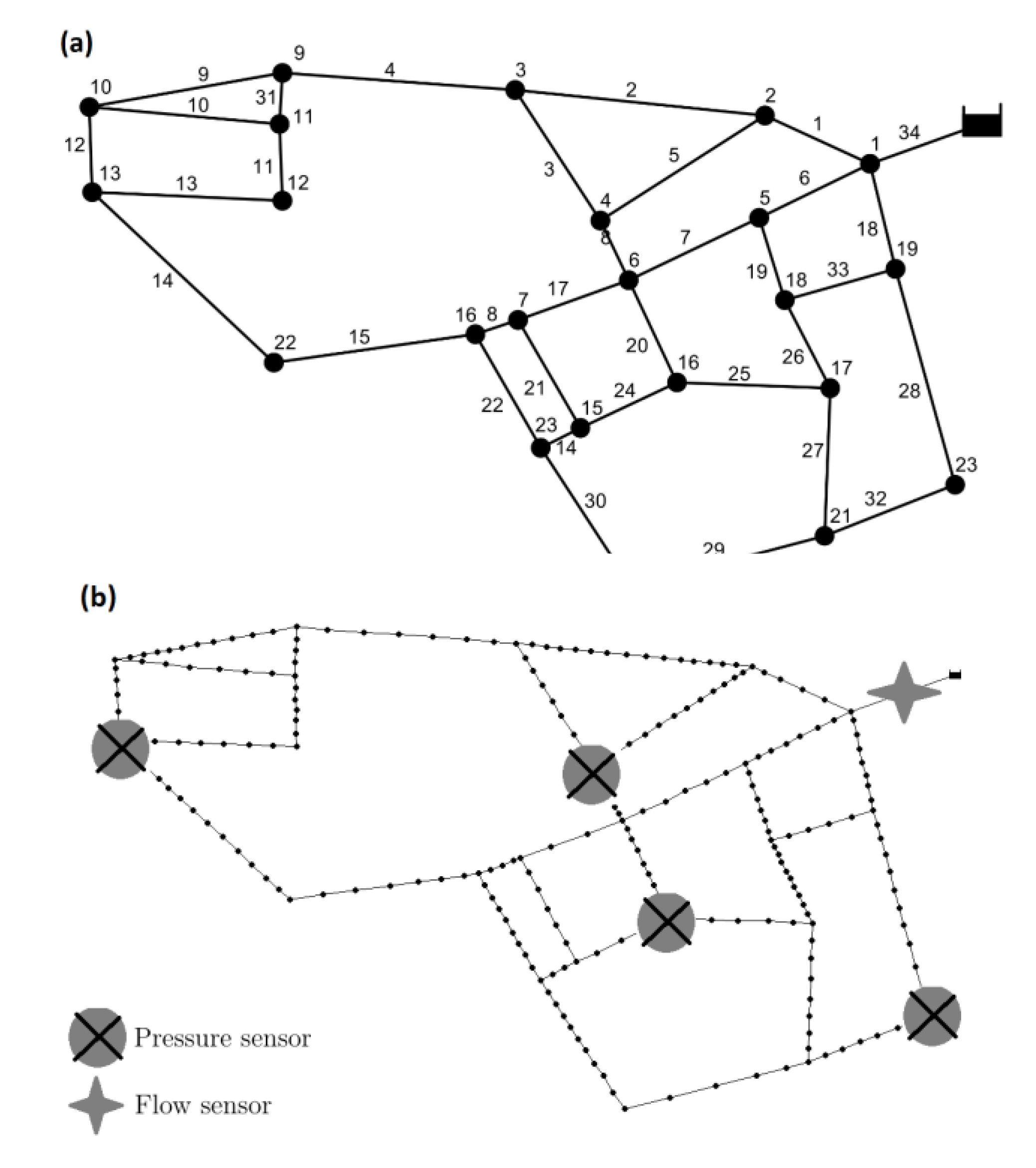
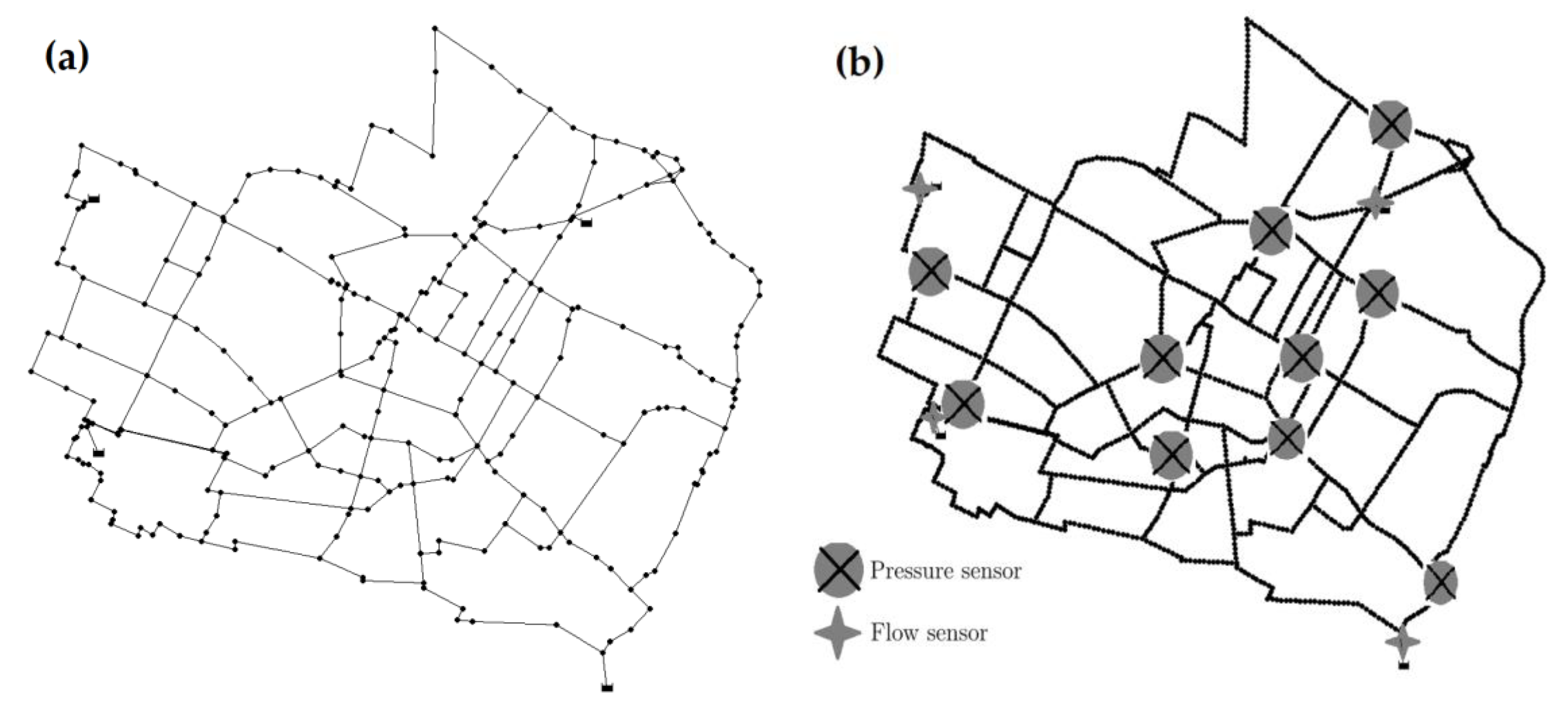
In this paper, the so-called Apulian network [38] is used for testing the proposed calibration procedure. Figure 2a shows the original Apulian network layout, which consists of 1 reservoir, 23 nodes and 34 pipes. This network is a representation of the real WDN through the skeletonised model. This network is selected because it can be considered as a medium-small network with a non-complex topology. In addition, this network is affected by a pressure deficit which is a common condition in many distribution systems. More information about this network is in [38]. In order to have measurements for the calibration procedure, a detailed network (Figure 2b) has been built following the procedure in Section 3.1. It consists of 1 reservoir, 238 nodes and 268 pipes. Since the paper is focused on the ill-posed calibration, only a low number of measured points are selected according to Section 3.1.
3.1. Data Generation and Sensor Placement
The purpose of this subsection is to describe the adopted procedure for generating the reference network and the sensors positioning. The former is necessary to compare the different models result during the proposed calibration procedure, while the latter enables to perform the calibration with a few known variables in some points of the network.
Hydraulic models are representations of real WDNs, where the withdrawals of the users are spread throughout the distribution network. Generally, the distance between consecutive withdrawals points depends on urban population density and its spatial distribution. It can range from a few dozen to hundreds meters. Therefore, a reference network is generated starting from the original Apulian model, where all the nodes have a random distance between 20 and 45 m. The amount of water demand is distributed randomly with the only constraint of mass balance at every single pipe [40]. Moreover, the roughness values are fixed considering a random pipes age between 20 and 50 years using the formulation of Colebrook and White reported in [41].
The method used to select the measurement locations has been proposed by [42] and four nodes and one pipe are selected to monitor pressure and flow rate, respectively. The methodology to sensor placement considered a localisation of the best measurement points based on a two stages analysis. The first is related to the sensitivity analysis of the nodes at leakages and consist on a calculation of a sensitivity matrix by placing a known leakage into each pipe and recording for each hour of a day the pressure. The sensitivity matrix is built for each hour of the day and so that each element represents the percentage variation of the pressure at the measurement’s node with respect to the nominal case where no leakage is placed in the network. Then a feature reduction is made by calculating four performance indexes representing the mean of the mean percentage pressure variations across different positions of the leakages, the variance across the day, the mean across the whole day and the variance across the whole day. Through a principal component analysis, the most sensitive nodes are extracted. The second step is a correlation analysis whose aim is to find the most sensitive and uncorrelated locations. Deeper information about the procedure can be found in [42].
Table 1 presents the reference data to perform the calibration problem. In addition, a pressure driven approach is used to have reference pressure values and reference flow rate values closer to reality. In particular, a nodal demand representation is adopted due to the correspondence of withdrawals and connection pipes in the reference network.
3.2. Results and Discussion
This section presents the result of the proposed calibration procedure using the four hydraulic approaches. To achieve a proper calibrated model, the simulated pressure at each node and the flow rate at each pipe have to match the reference network, which tries to represent the actual behaviour of the network.
A number of 100 runs of the optimisation algorithm is considered enough to converge to a stable solution as can be recognised looking at Figure 3a,b, where the pressure and flow rate Mean Absolute Error (MAE) is reported respectively, as a function of the number of runs, for the DPD approach. The plots show that after about 30 runs the MAE values stabilise toward an almost constant value.
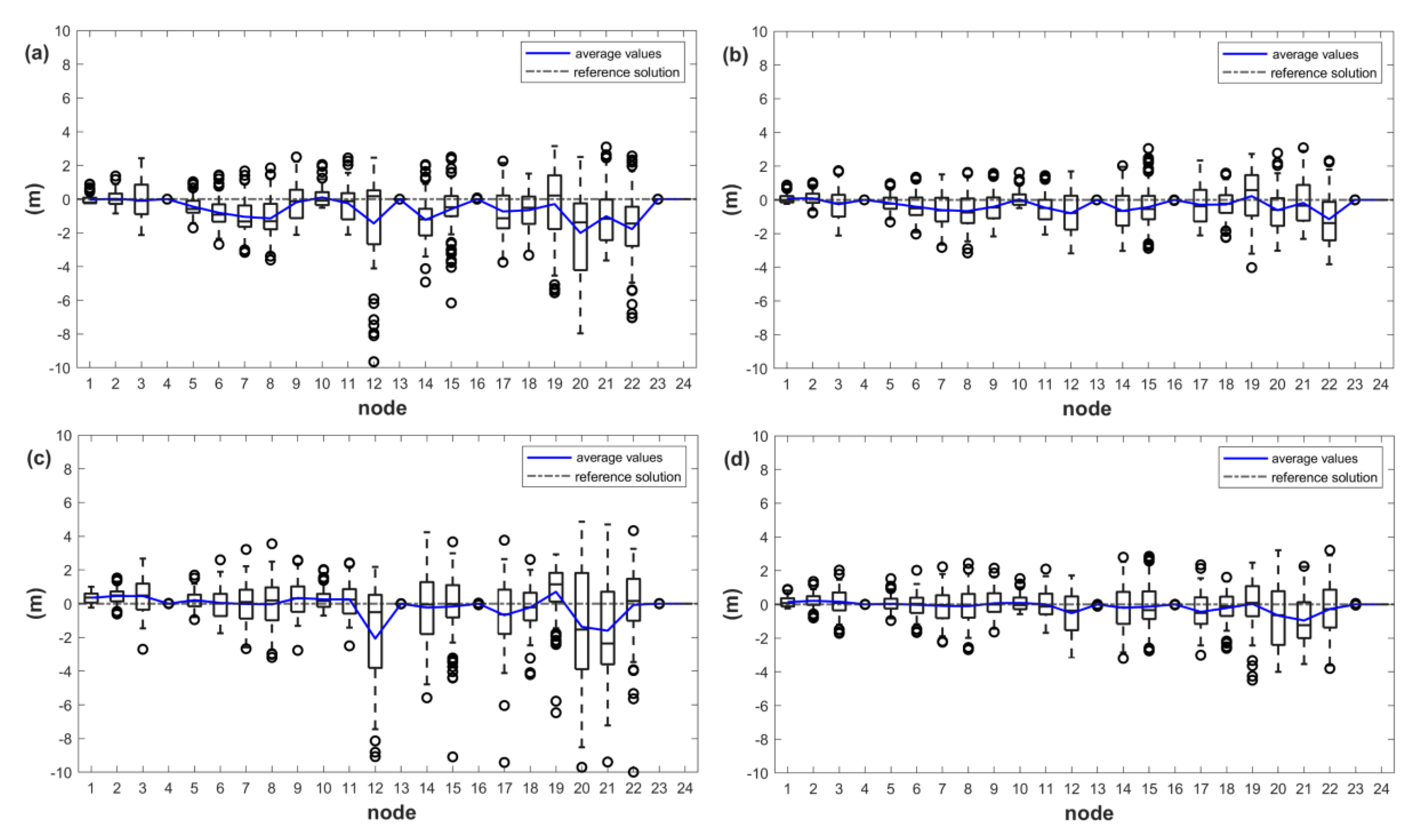
The results in terms of the difference between values in the reference network and in the calibrated models are reported under a Box and Whiskers plot. Figure 4 reports the pressure absolute error at each node, defined as the difference between the pressure at the node as from calibration procedure and pressure reference value at the node, and Figure 5 the flow rate absolute error related to the flow rate at each pipe.
Figure 4 shows the pressure results at each node of the 100 runs for the four hydraulic models in the different panels. It is observed that all the 100 runs of the four approaches converged to an optimum since in the nodes taken as measurements points (4, 13, 16 and 23) the simulated pressure is the same of the reference network (i.e., reference solution). As expected, the simulated pressure of the other nodes is fluctuating around the reference values due to the non-uniqueness problem of the solutions. This fluctuation appears to increase in case of hydraulic model formulated with a demand driven approach (Figure 4a,c with Figure 4b,d). For instance, the variability of the simulated pressure at node 12 has a range of 15.9 m with an NDD model and 15.6 m with a DDD. Contrary, the pressure obtained at the same node with a pressure driven approach has a variability of 4.87 m with an NPD and 4.84 m with a DPD. This behaviour can be ascribed to the inability of the demand driven models to simulate WDNs in pressure deficit condition.
Comparing Figure 4a,c with Figure 4b,d, it can be seen that the pressure of the average values of the pressure driven approach approximates better the reference solution than the demand driven one. In fact, the line representing the error of the average values of the NPD and DPD shows less error excursion at each node compared to the NDD and DDD ones. Moreover, the MAE of the average values compared with the reference solution are reported in the second column of Table 2. For each demand representation (i.e., concentrated at the nodes and distributed along pipes) the pressure driven approach halved the error compared to the demand driven ones. It can be noticed that the lowest MAE for the averaged values is reached by the DPD.
In addition, the solution that among the 100 runs achieved the lowest MAE compared with the reference network are also reported for each hydraulic approach. These are called the best solutions and the MAE are shown in the first column of Table 2. It is worth noting that the best solutions are not identifiable during a real calibration because clearly the reference network is unknown by definition. In this case, the best solutions are useful as a comparison to test the performances of the proposed methodology.
Then, a final solution is achieved by using as measurements data the mean values of the 100 runs of the calibrator of both node pressures and pipe flow rates. This is performed for the four hydraulic approaches and the MAE values are reported in the third column of Table 2. The importance of this last step is to have a model that is physically based, even if the error for these final solutions is slightly worst compared to one of the average values. For instance, the final DPD model makes a mean error of 0.24 m (1.5%) for each node compared to the 0.19 m (1.2%) of the average values.
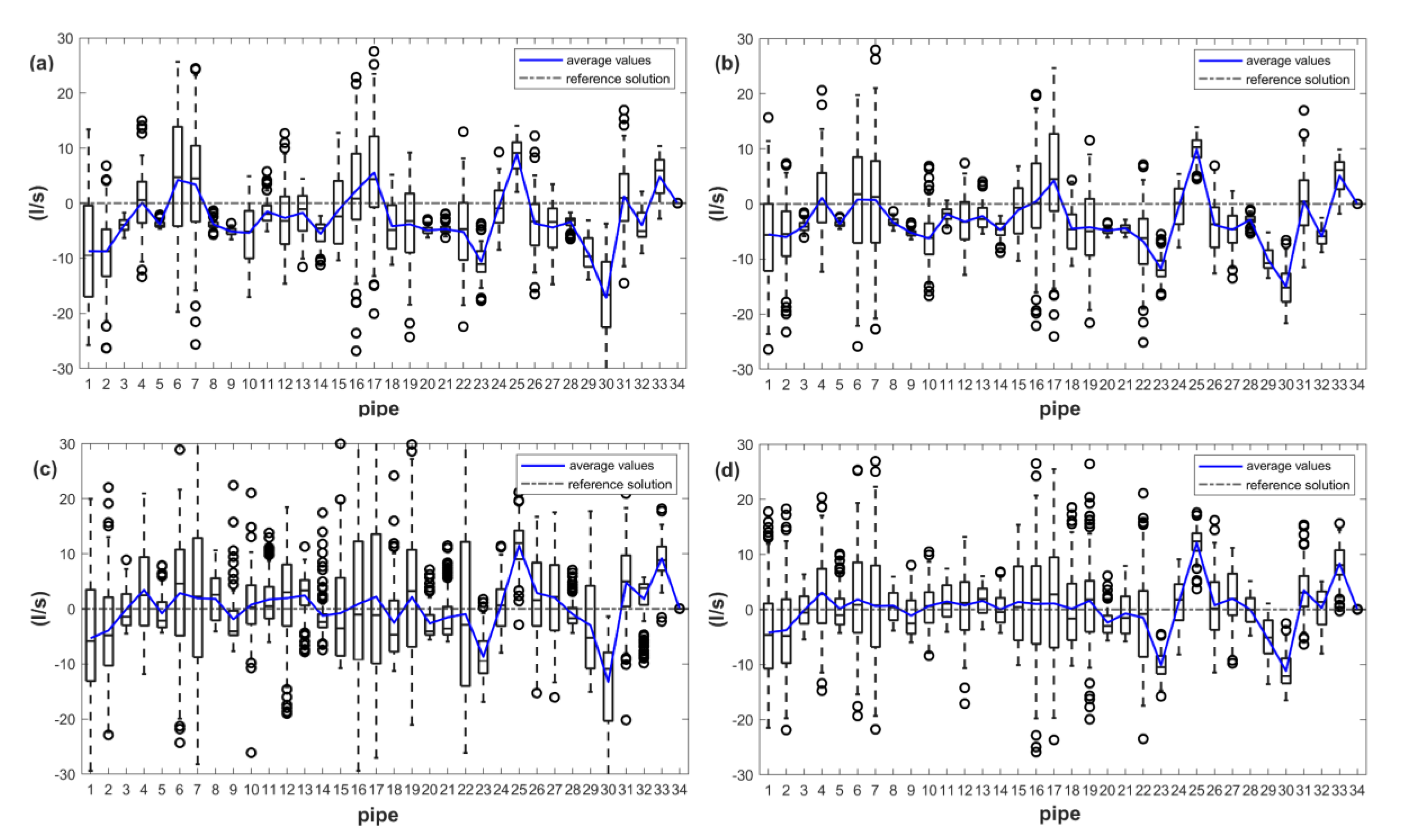
For the flow rate sides, Figure 5 shows the flow rate error at each pipe for each hydraulic approach in the different panels. The convergence of the solutions can be noticed in the measurement point (pipe 34), where the flow rate is matching the reference solution. Since only one flow measurement is available, the ill-posed problem is more underlined. Consequently, the dispersion of the error related to the flow rate is generally higher than the pressure fluctuation. For instance, the reference flow rate in pipe 17 is 62.34 L/s. The 100 runs of the calibration with the NDD approach ranged from 42 L/s to 96 L/s, with the NPD from 38 L/s to 87 L/s, with the DDD from 26 L/s to 110 L/s and with the DPD from 30 L/s to 87 L/s. Despite the significant dispersion of the 100 runs results, the average values are a good estimator. In fact, the considered pipe presents flow rate values of 67.9 L/s with the NDD, 66.6 L/s with the NPD, 64.5 L/s with the DDD and 63.45 L/s with the DPD.
The Apulian network presents flow rate inversion in some locations (e.g., pipes 20, 21, 23). The reference network is built as a real system with a dense spatial distribution of the withdrawals, while the models that are used from the calibrator are skeletonised. For this reason, none of the models formulated with water demands aggregated on the nodes (i.e., NDD and NPD) is able to match the real solution in the pipe affected by flow inversion. Despite the capability of distributed approaches (i.e., DDD and DPD) to detect the pipe inversion, it is a hard task due to the lack of measurements. In fact, the average values present its worst performance in the pipes affected by the flow rate inversion. The averaged values of the 100 runs of both the distributed approaches achieved a better result compared to the concentrated ones. Table 3 shows how the distributed demand representation improves the performance of the calibrated model in terms of flow rate. Specifically, the DPD achieved significantly the lowest MAE.
Table 2 and Table 3 show that the MAEs of the final solution with the DPD approach are smaller compared to the MAEs of the Best solution. Given that the best solution is obtained by optimisation process on a few known values, it can happen that in some point the estimated values (of the flow rate and/or pressure values) can be far from the local “true” value. Therefore, given that the average values are obtained by averaging the results (pressure at the nodes in Table 2 and flow rates at the pipes in Table 3) at all the network of the 100 runs, the average values can show lower MAE values with respect to the best solutions. In other words, calibrating with respect to the average values allows to achieve a more robust and performant solution than calibrating just on the few measurement points in a context of lack of measurements.
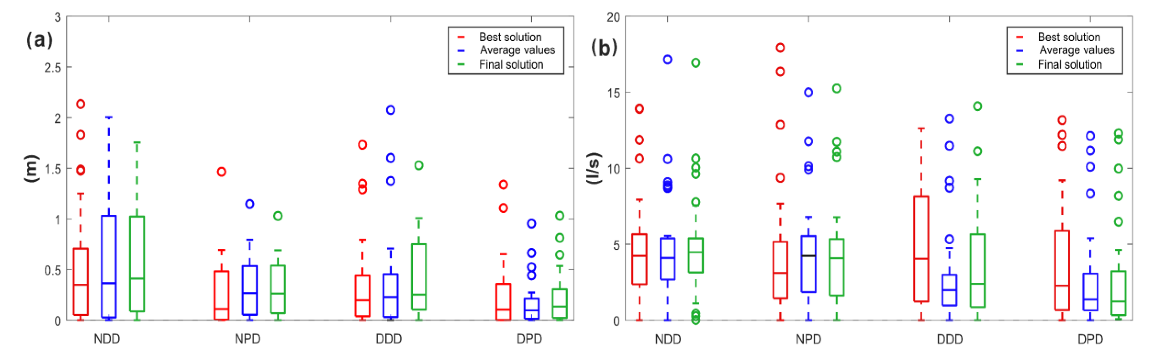
A comparison between the best solution and the average values among the 100 runs and the final solution is shown in Figure 6. This figure presents the three different solutions for each hydraulic approach divided into four groups. The absolute errors regarding the pressure at each node are reported under Box and Whisker plot in Figure 6a, and the absolute errors regarding the flow rate at each pipe in Figure 6b. It is clear that the four approaches reach different performance due to the two-breakthrough introduced in WDNs modelling in the last decade, which are distributed pipe demand and pressure driven approach. Therefore, the NDD approach, which presents none of these improvements, shows the worst performance in terms of Mean Absolute Error and error dispersion. On the contrary, the NPD and DDD approach, which presents only one of the two improvements, perform better than the NDD both for pressure and flow rate results. Nonetheless, the DPD approach, which assumes both distributed along pipes and pressure driven demand, achieve the lowest error both in terms of dispersion and mean.
The final solution shown in Figure 6, has performance comparable to the average values. Furthermore, this solution obtained with a DPD approach is capable of making a mean of 0.24 m of pressure error at the nodes and a mean of 2.55 L/s at each pipe, being a good estimation of the reference solution.
To evaluate the goodness of the selection of the average of 100 runs to perform the proposed calibration procedure, it is applied the statistical t-test. This test allows to verify whether the average value of the distribution of the 100 runs deviates significantly from the reference solution. The test is applied to each collected set of pressure and set of flow rate at each node and pipes, respectively. Given a significant level alpha of 0.01 and 99 degrees of freedom, concerning the pressure distribution, the null hypothesis is rejected in 25% of the cases and concerning the flow rate is rejected in 44% of the cases. In general, the mean is a good estimator of the reference solution but in some cases, where the test is rejected, the 100 runs distribution do not represent the reference solution. This happens due to the lack of measurement points of the ill-posed problem. It is also worth noting that most of the cases regarding the flow rate, where the test is rejected, are affected by the flux inversion problem previously described. The t-test has also been applied to the other hydraulic approaches highlighting worse results. The null hypothesis rejection values are 60% and 80% for the NDD approach, 65% and 76% for the NPD approach and 47% and 58% for the DDD approach concerning the pressure and flow rate distribution, respectively.
To highlight the reliability of the selection of the average with the DPD calibrated model, the confidence intervals are calculated by multiplying the standard error of the mean with the inverse value of the t-distribution with 0.99 probability and with 99 degrees of freedom. In Figure 7a,b are reported the results with the confidence intervals for the calibrated pressure at the nodes and the calibrated flow rate at the pipes, respectively.
In fact, as reported in Figure 7a, the reference solution is well bounded by the confidence intervals. On the contrary, Figure 7b shows the higher uncertainty according to the presence of just one flow rate measurement. However, as demonstrated by the t-test, the final calibrated with the DPD approach can be considered a consistent solution in a context of lack of measurements.
For the other hydraulic approaches, the statistical t-test has significantly inferior performance, meaning that, as already reported, the DPD performs better compared to the other approaches.
4. Test Case 2
To test the robustness of the proposed calibration, it is proposed a second test case based on a larger network, which is the Modena one [43]. According to Section 3.1, a detailed network is built and showed in Figure 8b, whereas Figure 8a shows the original Modena network layout and consists of 4 reservoirs, 267 nodes and 317 pipes. Following the procedure described in Section 3.1, ten pressure sensors and four flow rate sensors are placed.
Results and Discussion
The second test case aims to test the capability of the proposed methodology to handle larger networks. The pressure at the nodes and the flow rates at the pipes resulting from the calibration procedure are displayed in Figure 9a,b, respectively. Only the DPD approach is selected for this analysis due to the best performances already highlighted in the previous test case.
Despite the size of Modena network is higher than that of Apulian one, also in this case, a number of 100 runs of the optimisation algorithm is considered enough to converge to a stable solution. In particular, Figure 9a shows the pressure distribution of the 100 runs, the reference solution, the average values and the final solution. It is worth noting that the final solution follows the behaviour of the reference one leading to a good approximation in the context of an ill-posed problem. The mean absolute percentage error of the final calibrated model related to the pressure at each node results 4.4% (i.e., a mean of 0.9 m pressure error for each node), which can be considered as a robust solution for such a large network. Figure 9b displays the flow rate distribution. As for the pressure distribution, the final calibrated model well resembles the flow rate of the reference solution.
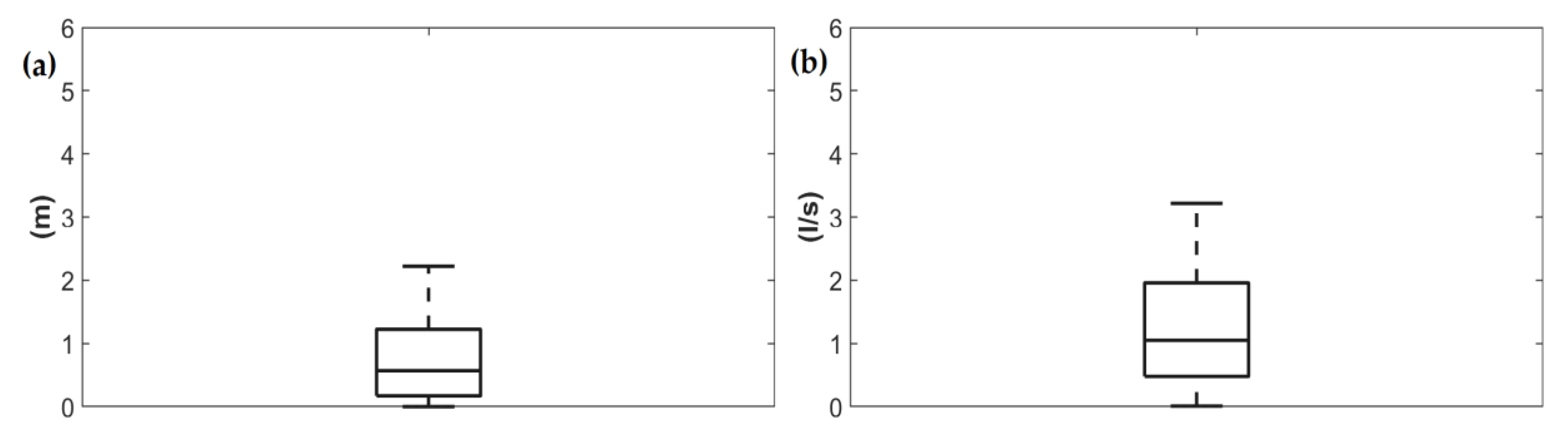
The absolute errors regarding the pressure at each node are reported under Box and Whisker plot in Figure 10a and regarding the flow rate at each pipe in Figure 10b.
The computational effort required for the 100 runs for this network is approximately three times higher than the time required for the Apulian. Nevertheless, the final calibrated model can be considered as a consistent starting point for network management.
5. Conclusions
This study proposes a multi-objective procedure to deal with the ill-posed calibration problem in WDNs. The whole calibration process has been developed considering a reduced number of measurements, as typically happen in reality. A procedure based on sensitivity and correlation analysis has been used to choose the optimal position to place pressor sensors. To overcome the non-uniqueness of the solution problem, 100 runs of the calibrator have been performed to obtain the average values. Therefore, it has been proposed a final solution that is achieved by using pressures and flows from the average values as measurements during the last run of the calibrator. This allows to have a model with almost the same performances of the average values of the 100 runs. To test the appropriate selection of the average, a Student t-test has been performed. The final solution of the proposed calibration methodology overcomes the non-uniqueness problem being also physically based on a set of pipe roughness and water demand. To evaluate the calibration procedure, a test case based on the Apulian network has been used. In particular, the reference network has been built in order to resemble a real system with a realistic spatial distribution of the withdrawals. In addition, to test the robustness of the proposed procedure, a second test case based on the larger Modena network has been proposed.
A comparison among the calibration process of four WDN simulation approaches ((1) nodal demand driven; (2) nodal pressure driven; (3) distributed demand driven; (4) distributed pressure driven) has been carried out. It has been proved that the selection of the more reliable hydraulic approach to simulate a real system can significantly improve the result of the calibration. In particular, the better performance of the distributed pressure driven approach based emerged. Future efforts will address the problem of the computational requirements, which are intensive for a large network like the Modena one, and also will involve the problem of the leakage presence and of the measurements noise in a real network. Despite that, this calibration procedure can be replicable in WDNs due to its capability to address the problems of lack of measurements and pressure deficit condition, which are common in real systems worldwide.
Author Contributions
Conceptualization, A.Z., A.M., S.S. and M.R.; data curation, A.Z.; funding acquisition, M.R.; investigation, A.Z.; methodology, A.Z., A.M. and S.S.; software, A.Z.; supervision, M.R.; validation, A.Z. and A.M.; writing-original draft, A.Z.; writing-review and editing, A.Z., A.M., S.S. and M.R. All authors have read and agreed to the published version of the manuscript.
Funding
Part of this research has been carried out under the project “Applied Thermo-Fluid Dynamics Laboratories, Applied Research Infrastructures for Companies and Industry in South Tyrol” (FESR1029), financed by the European Regional Development Fund (ERDF) Investment for Growth and Jobs Programme 2014–2020 and the Autonomous Province of Bolzano. This work has been also partially carried out within the Research project “AI-ALPEN”, CUP: B26J16000300003 funded by the PAB (Autonomy Provence of Bozen-Italy) for University Research-2014.
Conflicts of Interest
The authors declare no conflict of interest.
References
- Savic, D.; Kapelan, Z.S.; Jonkergouw, P.M. Quo vadis water distribution model calibration? Urban Water J. 2009, 6, 3–22. [Google Scholar] [CrossRef]
- Walski, T.M. Technique for Calibrating Network Models. J. Water Resour. Plan. Manag. 1983, 109, 360–372. [Google Scholar] [CrossRef]
- Bhave, P.R. Calibrating Water Distribution Network Models. J. Environ. Eng. 1988, 114, 120–136. [Google Scholar] [CrossRef]
- Ormsbee, L.E.; Wood, D.J. Explicit Pipe Network Calibration. J. Water Resour. Plan. Manag. 1986, 112, 166–182. [Google Scholar] [CrossRef]
- Di Nardo, A.; Di Natale, M.; Gisonni, C.; Iervolino, M. A genetic algorithm for demand pattern and leakage estimation in a water distribution network. J. Water Supply Res. Technol. 2014, 64, 35–46. [Google Scholar] [CrossRef]
- Do, N.C.; Simpson, A.R.; Deuerlein, J.W.; Piller, O. Calibration of Water Demand Multipliers in Water Distribution Systems Using Genetic Algorithms. J. Water Resour. Plan. Manag. 2016, 142, 04016044. [Google Scholar] [CrossRef]
- Tabesh, M.; Jamasb, M.; Moeini, R. Calibration of water distribution hydraulic models: A comparison between pressure dependent and demand driven analyses. Urban Water J. 2011, 8, 93–102. [Google Scholar] [CrossRef]
- Wu, Z.Y.; Walski, T.; Mankowski, R.; Herrin, G.; Gurrieri, R.; Tryby, M. Calibrating water distribution model via genetic algorithms. In Proceedings of the 2002 AWWA IMTech Conference, Kansas City, MO, USA, 14–17 April 2002. [Google Scholar]
- Laucelli, D.; Berardi, L.; Giustolisi, O.; Vamvakeridou-Lyroudia, L.S.; Kapelan, Z.; Savic, D.; Barbaroand, G. Calibration of Water Distribution System Using Topological Analysis. In Water Distribution Systems Analysis; American Society of Civil Engineers: Tucson, AZ, USA, 2011; pp. 1664–1681. [Google Scholar] [CrossRef]
- Asadzadeh, M.; Tolson, B.A.; McKillop, R. A Two Stage Optimization Approach for Calibrating Water Distribution Systems. In Water Distribution Systems Analysis; American Society of Civil Engineers: Tucson, AZ, USA, 2011; pp. 1682–1694. [Google Scholar] [CrossRef]
- Meirelles, G.; Manzi, D.; Brentan, B.M.; Goulart, T.; Junior, E.L. Calibration Model for Water Distribution Network Using Pressures Estimated by Artificial Neural Networks. Water Resour. Manag. 2017, 31, 4339–4351. [Google Scholar] [CrossRef]
- Do, N.C.; Simpson, A.R.; Deuerlein, J.; Piller, O. Particle Filter–Based Model for Online Estimation of Demand Multipliers in Water Distribution Systems under Uncertainty. J. Water Resour. Plan. Manag. 2017, 143, 04017065. [Google Scholar] [CrossRef] [Green Version]
- Zhou, X.; Xu, W.; Xin, K.; Yan, H.; Tao, T. Self-Adaptive Calibration of Real-Time Demand and Roughness of Water Distribution Systems. Water Resour. Res. 2018, 54, 5536–5550. [Google Scholar] [CrossRef]
- Hutton, C.J.; Kapelan, Z.; Vamvakeridou-Lyroudia, L.; Savic, D. Dealing with Uncertainty in Water Distribution System Models: A Framework for Real-Time Modeling and Data Assimilation. J. Water Resour. Plan. Manag. 2014, 140, 169–183. [Google Scholar] [CrossRef]
- Puust, R.; Kapelan, Z.; Savic, D.; Koppel, T. A review of methods for leakage management in pipe networks. Urban Water J. 2010, 7, 25–45. [Google Scholar] [CrossRef]
- Covelli, C.; Cozzolino, L.; Cimorelli, L.; Della Morte, R.; Pianese, D. A model to simulate leakage through joints in water distribution systems. Water Supply 2015, 15, 852–863. [Google Scholar] [CrossRef]
- Covelli, C.; Cimorelli, L.; Cozzolino, L.; Della Morte, R.; Pianese, D. Reduction in water losses in water distribution systems using pressure reduction valves. Water Supply 2016, 16, 1033–1045. [Google Scholar] [CrossRef] [Green Version]
- Kang, D.; Lansey, K. Demand and Roughness Estimation in Water Distribution Systems. J. Water Resour. Plan. Manag. 2011, 137, 20–30. [Google Scholar] [CrossRef]
- Letting, L.; Hamam, Y.; Abu-Mahfouz, A.M. Estimation of Water Demand in Water Distribution Systems Using Particle Swarm Optimization. Water 2017, 9, 593. [Google Scholar] [CrossRef] [Green Version]
- Rossman, L.A. EPANET 2: Users Manual. 2000. Available online: https://epanet.es/wp-content/uploads/2012/10/EPANET_User_Guide.pdf (accessed on 15 January 2020).
- Sophocleous, S.; Savic, D.; Kapelan, Z.; Giustolisi, O. A Two-stage Calibration for Detection of Leakage Hotspots in a Real Water Distribution Network. Procedia Eng. 2017, 186, 168–176. [Google Scholar] [CrossRef]
- Todini, E.; Pilati, S. A gradient algorithm for the analysis of pipe networks. In Computer Applications in Water Supply: Vol. 1—Systems Analysis and Simulation; Research Studies Press Ltd.: Baldock, UK, 1988; pp. 1–20. [Google Scholar]
- Collins, M.; Cooper, L.; Helgason, R.; Kennington, J.; Leblanc, L. Solving the Pipe Network Analysis Problem Using Optimization Techniques. Manag. Sci. 1978, 24, 747–760. [Google Scholar] [CrossRef]
- Giustolisi, O.; Savic, D.; Kapelan, Z. Pressure-Driven Demand and Leakage Simulation for Water Distribution Networks. J. Hydraul. Eng. 2008, 134, 626–635. [Google Scholar] [CrossRef] [Green Version]
- Siew, C.; Tanyimboh, T.T. Pressure-Dependent EPANET Extension. Water Resour. Manag. 2012, 26, 1477–1498. [Google Scholar] [CrossRef] [Green Version]
- Berardi, L.; Giustolisi, O.; Todini, E. Accounting for uniformly distributed pipe demand in WDN analysis: Enhanced GGA. Urban Water J. 2010, 7, 243–255. [Google Scholar] [CrossRef]
- Menapace, A.; Avesani, D.; Righetti, M.; Bellin, A.; Pisaturo, G.R. Uniformly Distributed Demand EPANET Extension. Water Resour. Manag. 2018, 32, 2165–2180. [Google Scholar] [CrossRef]
- Menapace, A.; Avesani, D. Global Gradient Algorithm Extension to Distributed Pressure Driven Pipe Demand Model. Water Resour. Manag. 2019, 33, 1717–1736. [Google Scholar] [CrossRef] [Green Version]
- Todini, E. Extending the global gradient algorithm to unsteady flow extended period simulations of water distribution systems. J. Hydroinform. 2010, 13, 167–180. [Google Scholar] [CrossRef] [Green Version]
- Avesani, D.; Righetti, M.; Righetti, D.; Bertola, P. The extension of EPANET source code to simulate unsteady flow in water distribution networks with variable head tanks. J. Hydroinform. 2012, 14, 960–973. [Google Scholar] [CrossRef] [Green Version]
- Deb, K.; Agrawal, S.; Pratap, A.; Meyarivan, T. A fast elitist non-dominated sorting genetic algorithm for multi-objective optimization: NSGA-II. In International Conference on Parallel Problem Solving from Nature; Springer: Berlin/Heidelberg, Germany, 2000; pp. 849–858. [Google Scholar]
- Germanopoulos, G. A technical note on the inclusion of pressure dependent demand and leakage terms in water supply network models. Civ. Eng. Syst. 1985, 2, 171–179. [Google Scholar] [CrossRef]
- Gupta, R.; Bhave, P.R. Comparison of Methods for Predicting Deficient-Network Performance. J. Water Resour. Plan. Manag. 1996, 122, 214–217. [Google Scholar] [CrossRef]
- Tanyimboh, T.T.; Templeman, A.B. Seamless pressure-deficient water distribution system model. Proc. Inst. Civ. Eng.-Water Manag. 2010, 163, 389–396. [Google Scholar] [CrossRef] [Green Version]
- Wu, Z.Y.; Clark, C. Evolving Effective Hydraulic Model for Municipal Water Systems. Water Resour. Manag. 2008, 23, 117–136. [Google Scholar] [CrossRef]
- Siew, C.; Tanyimboh, T.T. Augmented Gradient Method for Head Dependent Modelling of Water Distribution Networks. In World Environmental and Water Resources Congress 2009: Great Rivers; American Society of Civil Engineers: Kansas City, MO, USA, 2009; pp. 1–10. [Google Scholar] [CrossRef]
- Giustolisi, O.; Kapelan, Z.; Savic, D. Extended Period Simulation Analysis Considering Valve Shutdowns. J. Water Resour. Plan. Manag. 2008, 134, 527–537. [Google Scholar] [CrossRef]
- Giustolisi, O.; Todini, E. On the approximation of distributed demands as nodal demands in WDN analysis. In Proceedings of the XXXI National Hydraulics and Hydraulic Construction Conference, Perugia, Italy, 9–12 September 2008. [Google Scholar]
- Giustolisi, O.; Todini, E. Pipe hydraulic resistance correction in WDN analysis. Urban Water J. 2009, 6, 39–52. [Google Scholar] [CrossRef]
- Menapace, A.; Righetti, M.; Avesani, D. Application of Distributed Pressure Driven Modelling in Water Supply System. In Proceedings of the WDSA/CCWI Joint Conference Proceedings, Kingston, ON, Canada, 23–25 July 2018. [Google Scholar]
- Sharp, W.W.; Walski, T.M. Predicting Internal Roughness in Water Mains. J. Am. Water Work. Assoc. 1988, 80, 34–40. [Google Scholar] [CrossRef] [Green Version]
- Righetti, M.; Bort, C.M.G.; Bottazzi, M.; Menapace, A.; Zanfei, A. Optimal Selection and Monitoring of Nodes Aimed at Supporting Leakages Identification in WDS. Water 2019, 11, 629. [Google Scholar] [CrossRef] [Green Version]
- Bragalli, C.; D’Ambrosio, C.; Lee, J.; Lodi, A.; Toth, P. Water Network Design by MINLP; Rep No RC24495; IBM Res.: Yorktown Heights, NY, USA, 2008. [Google Scholar]
Figure 1.
Calibration procedure flow-chart.

Figure 2.
Apulian network: (a) model network where the calibration processes are launched (number of nodes = 23, number of pipes = 34); (b) reference network where the measurements are taken (number of nodes = 238, number of pipes = 268).
Figure 2.
Apulian network: (a) model network where the calibration processes are launched (number of nodes = 23, number of pipes = 34); (b) reference network where the measurements are taken (number of nodes = 238, number of pipes = 268).

Figure 3.
Behaviour of the Mean Absolute Errors (MAEs), calculated as the difference between average values and values of the reference network, of the distributed pressure driven (DPD) approach, with respect to the number of runs. In panel (a) is displayed the MAE related to the pressures and in panel (b) is displayed the MAE related to the flow rates.

Figure 4.
Pressure errors (i.e., the difference between simulated and reference values) at each node of the 100 runs for each hydraulic approach: (a) NDD; (b) NPD; (c) DDD; (d) DPD. The error of the average values (i.e., average values line) is also displayed in each plot.
Figure 4.
Pressure errors (i.e., the difference between simulated and reference values) at each node of the 100 runs for each hydraulic approach: (a) NDD; (b) NPD; (c) DDD; (d) DPD. The error of the average values (i.e., average values line) is also displayed in each plot.

Figure 5.
Flow rate errors (i.e., the difference between simulated and reference values) at each pipe of the 100 runs for each hydraulic approach: (a) NDD; (b) NPD; (c) DDD; (d) DPD. The error of the average values (i.e., average values line) is also displayed in each plot.
Figure 5.
Flow rate errors (i.e., the difference between simulated and reference values) at each pipe of the 100 runs for each hydraulic approach: (a) NDD; (b) NPD; (c) DDD; (d) DPD. The error of the average values (i.e., average values line) is also displayed in each plot.

Figure 6.
Comparison of the solutions. (a) Pressure absolute errors; (b) flow rate absolute errors. Error distribution of the best solution among the 100 runs (left box); average values (middle box); final solution (right box).
Figure 6.
Comparison of the solutions. (a) Pressure absolute errors; (b) flow rate absolute errors. Error distribution of the best solution among the 100 runs (left box); average values (middle box); final solution (right box).

Figure 7.
Resulting solution in the Apulian network with the DPD approach. In panel (a) are displayed the pressure distribution of the 100 runs, the reference values, the average values and the final one with confidence intervals. The flow rate distribution of the 100 runs, the reference values, the average values and the final one with confidence intervals are displayed in panel (b).

Figure 8.
Modena network: (a) model network where the calibration processes are launched; (b) reference network where the measurements are taken.
Figure 8.
Modena network: (a) model network where the calibration processes are launched; (b) reference network where the measurements are taken.

Figure 9.
Resulting calibration of the Modena network with the DPD approach. In panel (a) is displayed the pressure distribution of the 100 runs, the reference values, the average values and the final one. The flow rate distribution of the 100 runs is displayed in panel (b).
Figure 9.
Resulting calibration of the Modena network with the DPD approach. In panel (a) is displayed the pressure distribution of the 100 runs, the reference values, the average values and the final one. The flow rate distribution of the 100 runs is displayed in panel (b).

Figure 10.
Absolute errors calculated as the absolute difference between reference values and simulated values in the final calibrated model of the Modena network. Panel (a) is related to the pressure at each node and panel (b) to the flow rate at each pipe.
Figure 10.
Absolute errors calculated as the absolute difference between reference values and simulated values in the final calibrated model of the Modena network. Panel (a) is related to the pressure at each node and panel (b) to the flow rate at each pipe.


Table 1.
Measured flow rate (on the bottom) and measured pressure (on the top) data for the Apulian network.
Table 1.
Measured flow rate (on the bottom) and measured pressure (on the top) data for the Apulian network.
| Node (ID) | Pressure (m) |
|---|---|
| 4 | 17.92 |
| 13 | 13.37 |
| 16 | 16.55 |
| 23 | 13.57 |
| Pipe ID | Flow Rate (L/s) |
| 34 | 240.82 |
Table 2.
MAE regarding the simulated pressure of the Best solution, the Average values and the Final solution with respect to the reference network.
Table 2.
MAE regarding the simulated pressure of the Best solution, the Average values and the Final solution with respect to the reference network.
| Solution | Best Solution | Average Values | Final Solution | |
|---|---|---|---|---|
| Approach | (m) | (m) | (m) | |
| NDD | 0.57 | 0.60 | 0.62 | |
| NPD | 0.28 | 0.34 | 0.34 | |
| DDD | 0.52 | 0.41 | 0.46 | |
| DPD | 0.28 | 0.19 | 0.24 | |
Table 3.
MAE regarding the simulated flow rate of the Best solution, the Average values and the Final solution with respect to the reference network.
Table 3.
MAE regarding the simulated flow rate of the Best solution, the Average values and the Final solution with respect to the reference network.
| Solution | Best Solution | Average Values | Final Solution | |
|---|---|---|---|---|
| Approach | (L/s) | (L/s) | (L/s) | |
| NDD | 4.60 | 4.66 | 4.76 | |
| NPD | 4.29 | 4.33 | 4.34 | |
| DDD | 4.95 | 2.98 | 3.63 | |
| DPD | 3.57 | 2.49 | 2.55 | |
© 2020 by the authors. Licensee MDPI, Basel, Switzerland. This article is an open access article distributed under the terms and conditions of the Creative Commons Attribution (CC BY) license (http://creativecommons.org/licenses/by/4.0/).
Share and Cite
MDPI and ACS Style
Zanfei, A.; Menapace, A.; Santopietro, S.; Righetti, M. Calibration Procedure for Water Distribution Systems: Comparison among Hydraulic Models. Water 2020, 12, 1421. https://doi.org/10.3390/w12051421
AMA Style
Zanfei A, Menapace A, Santopietro S, Righetti M. Calibration Procedure for Water Distribution Systems: Comparison among Hydraulic Models. Water. 2020; 12(5):1421. https://doi.org/10.3390/w12051421
Chicago/Turabian StyleZanfei, Ariele, Andrea Menapace, Simone Santopietro, and Maurizio Righetti. 2020. "Calibration Procedure for Water Distribution Systems: Comparison among Hydraulic Models" Water 12, no. 5: 1421. https://doi.org/10.3390/w12051421
Note that from the first issue of 2016, this journal uses article numbers instead of page numbers. See further details here.