Remote-Sensing-Based Water Balance for Monitoring of Evapotranspiration and Water Stress of a Mediterranean Oak–Grass Savanna

Abstract

Mediterranean oak savannas (known as dehesas in Spain) are exposed to numerous threats from natural and economic causes. A close monitoring of the use of water resources and the status of the vegetation in these ecosystems can be useful tools for maintaining the production of ecological services. This study explores the estimation of evapotranspiration (ET) and water stress over a dehesa by integrating remotely sensed data into a water balance using the FAO-56 approach (VI-ET_o model). Special attention is paid to the different phenology and contribution to the system’s hydrology of the two main canopy layers of the system (tree + grass). The results showed that the model accurately reproduced the dynamics of the water consumed by the vegetation, with RMSE of 0.47 mm day⁻¹ and low biases for both, the whole system and the grass layer, when compared with flux tower measurements. The ET/ET_o ratio helped to identify periods of water stress, confirmed for the grassland by measured soil water content. The modeling scheme and Sentinel-2 temporal resolution allowed the reproduction of fast and isolated ET pulses, important for understanding the hydrologic behavior of the system, confirming the adequacy of this sensor for monitoring grasslands water dynamics.

1. Introduction

Water availability is the main climate factor limiting the primary production of Mediterranean agroforestry systems. Recurrent water scarcity conditions are likely to worsen, with a decrease in the quality, quantity, and resilience of freshwater resources predicted for the Mediterranean region under the current global change scenario [1,2]. In this context of increased variability, improved knowledge of hydrological process dynamics and its impact on vegetation is essential to reinforce ecosystem water resource management and planning, which may contribute to reducing vulnerability to climate change. Metrics describing the ecosystem’s status regarding water consumption and vegetation growth, as well as its general stability, can facilitate regular monitoring and the implementation of conservation strategies at different scales (regional, national, or European policies), while maintaining the productivity required to support the rural economy. Earth observation technologies provide timely and quantitative open data to assist in the calculation of these metrics at different resolutions.

Oak savannas growing in the Mediterranean region, known as dehesa in Spain and montado in Portugal, are structurally and physiologically adapted to survive under extreme seasonal water scarcity conditions, including high temperatures and soil dryness levels for several months every summer [3,4]. This landscape is a complex mosaic of widely-spaced oak trees (mostly Quercus Ilex L. and Quercus Suber L.), combined with pastures, shrubs, and crops. The low ground fractional coverage of the oak trees constrains the leaf area index (LAI) of the ecosystem and enables light to enter the understory, meaning that grass production can be maintained in these soils, usually with a low fertility [5]. In addition, scattered tree roots can explore a large volume of soil [6,7], with pasture tapping shallow water supplies. This structure imposes a marked spatial heterogeneity on the functioning of the ecosystem, with additional differences in the water use below and outside the tree canopy [8,9].

This human-induced ecosystem has historically offered a compromise between production and conservation, satisfying the population’s economic needs while providing multiple environmental services, such as biodiversity hotspots, landscape, water provisioning, or CO₂ fixation [10]. However, it is currently being exposed to numerous threats, such as the lack of the natural regeneration of tree species [11], its low profitability, the intensification of agricultural and livestock activities, and changes in soil properties and hydrological processes, increasing soil erosion [5,12]. The situation might worsen due to climate change, with prediction models forecasting warmer and drier summers, a growing occurrence of extreme high-temperature events and heatwaves [13,14], and increased drought frequency and intensity [15,16,17,18]. The abandonment of farmland and grazing areas due to the aforementioned processes will also trigger changes in land use and management [19,20], leading to an additional risk to dehesa conservation.

Remote sensing is widely used in agricultural areas to assist in the computation of crop water requirements, using an adaptation of the Food and Agriculture Organization (FAO) Irrigation and drainage paper -56 approach [21,22]. This model estimates crop evapotranspiration (ET) as being the product of reference evapotranspiration (ET_o), representing the atmospheric evaporative demand, and a crop coefficient (K_c) used to account for crop factors, such as crop type, developmental stage, ground cover, or soil water content. The integration of vegetation indices (VIs) derived from remote sensing into this model (herein called VI-ET_o) improves the estimation of canopy transpiration [23,24,25,26,27,28] and takes advantage of the spatial and temporal resolutions (daily, weekly, monthly) of remotely sensed data. Different approaches and applications of this method have been reviewed by Glenn et al. [29], Calera el al. [30], and Pôças et al. [31]. Applications over natural ecosystems are substantially fewer than over crops, and present additional difficulties due to the higher heterogeneity in plant properties. The adjustments proposed by Allen et al. [21] for using this method in native vegetation under water deficit conditions, and the good estimations of the vegetation ground cover fraction (f_c) and LAI produced by remote sensing over mixed vegetation types and natural ecosystems [32], are the basis for applications in non-cropped areas.

Previous studies have given good results in the application of VI-ET_o over savanna landscapes in Mediterranean and African semi-arid areas [33,34]. However, these studies highlighted the difficulty of taking into account the heterogeneity of the system in the estimation of effective model parameters. Another factor that needs to be considered in the use of this method over dehesas is the differential spectral response of holm oak trees (similar to olive trees) compared to other plant species under full cover conditions, which may condition ET and water stress monitoring when VI-based techniques are used [35]. On the other hand, Mateos et al. [36] underlined the importance of the accurate computation of f_c for incomplete canopies when applying this method. In this case, the frequent presence of a senescent or dead grass layer during the summer and the low tree cover, as the only photosynthetic vegetation during this season, might reduce the ability of broadband VIs to accurately estimate f_c in the dry period. Depending on the sensor and the spectra of the soils, the non-photosynthetic vegetation may be spectrally indistinguishable from the soil [37]. Xu et al. [38] found a linear relationship between Normalized Difference Vegetation Index (NDVI) and dead cover in grasslands, with a variable contribution to NDVI depending on the dead cover fraction. This study uses both measurements and models to explore the factors influencing the estimation of ET and water stress over a dehesa ecosystem in an attempt to provide effective vegetation parameters to model the water balance with the assistance of remote sensing. Special attention is paid to the different behavior and phenology of the two main canopy layers of the ecosystem (tree + grass) and to the varying contribution to the system’s hydrology. The use of layer-specific parameters and the effect of the non-photosynthetic vegetation on the modeling scheme are evaluated.

2. Materials and Methods

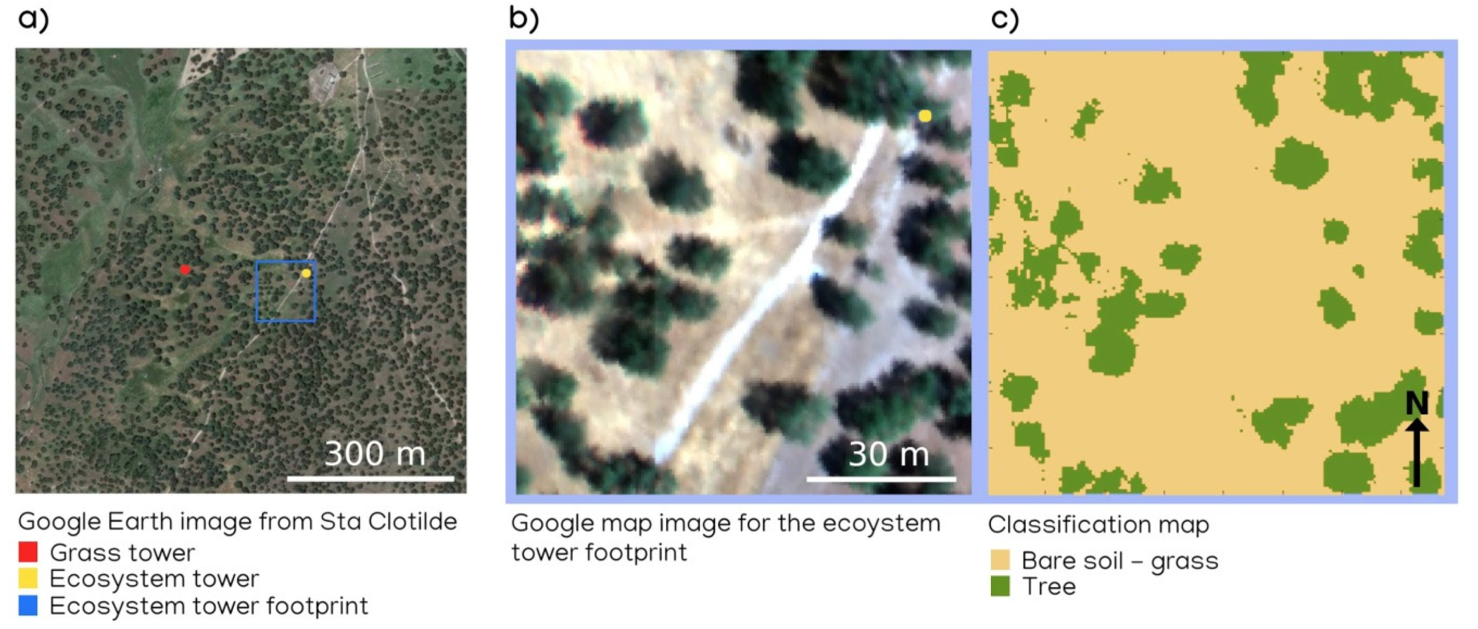
2.1. Study Site

The study was conducted over a dehesa farm (Santa Clotilde, 38°12′ N; 4°17′ W, 736 m a.s.l.; Figure 1a) located in the Natural Park of the Sierra de Cardeña y Montoro, in Southern Spain. It is a homogeneous landscape with gentle slopes and multiple uses (agriculture, extensive livestock grazing, and hunting). The continental Mediterranean climate of the area is characterized by a strong seasonality, with moderately cold winters alternating with long, hot, and dry summers. The rainfall presents intra- and interyear variability, with an annual average of 895 mm (from 1990 to 2015), concentrated during spring and fall.

The study site vegetation consists of widely-spaced oak trees (mostly Quercus ilex L., with a scattering of Quercus faginea Lam. and Quercus pyrenaica Willd. individuals) combined with a subcanopy composed of annual grassland. The layer of annual species emerges after the first rainfall in autumn and dries out in late spring. The majority of the herbaceous species belong to the Stellarieteamediae class, and more specifically to the Bromo scoparii-Hordeetumleporini association [39], according to field visual identification based on the work of Melendo [40]. This grass cover corresponds to annual ephemeral, ruderal, and nitrophilous weed communities as a result of moderately intense continuous grazing. The predominant species are: Bromus hordeaceus, Hordeum leporinum, Bromus diandrus, Echium plantagineum, Lolium rigidum, Anthemis arvensis, Plantago lagopus, Raphanus raphanistrum, Sisymbrium officinale, and Avena barbata.

In relation to the soil’s properties, the prevailing textural class in the area is sandy loam, with variations in soil depths generally ranging between 0.5 and 2.40 m. The bulk density increases linearly with depth, from a mean value of 1.3 Mg m⁻³ at the surface to 1.6 Mg m⁻³ at around 25–30 cm. This increase with depth is commonly linked to a lower C content and higher compaction, but in this area it is also related to the increase in stoniness [41].

2.2. Ground Validation Measurements

Ground validation measurements were taken at the study area using two eddy covariance towers (ECT), one over the combined tree + grassland system and another over open grassland (Figure 1b–d). Measurement sties to complement the flux towers data were located on two grazing exclusion enclosures, over open grassland and under a holm oak tree, to assess the heterogeneity of the study area. The setup encompasses all the instruments required for continuous measurement of all energy balance components, including the turbulent fluxes of sensible (H) and latent heat (LE), the net radiation (Rn), and the soil heat flux (G).

The ECT system over the dehesa was installed on a tower at a height of 18 m in April 2012, registering the ecosystem response as a whole (Figure 1c). A 3D sonic anemometer (model CSAT3 Campbell Scientific Inc., Logan, UT, USA) measuring horizontal and vertical fluctuations of temperature and wind speed, and a hygrometer (model KH20, Campbell Scientific Inc., Logan, UT, USA) used to estimate water vapor fluctuations were installed at the beginning, with the latter being replaced in 2015 by a LICOR-7500 open path CO₂/H₂O gas analyzer (IRGA; model LI-7500A, Li-Cor, Lincoln, NE, USA), taking simultaneous measurements of carbon dioxide and water vapor in turbulent air structures. These measurements were recorded with high frequency (10 Hz), and half-hourly averages were computed after applying corrections of density effects due to heat and water vapor transfer [42]. The net radiation was first obtained with a net radiometer (model NR-Lite, Kipp and Zonen, Delft, Netherlands), which was also replaced by a four-component net-radiometer (model NR01, Hukseflux Thermal Sensors, Delft, The Netherlands) in 2015. The relative humidity and air temperature were also measured with a probe (model HMP155, Vaisala, Helsinki, Finland). More information on the study area and the equipment can be found in the work of Andreu et al. [43].

The soil heat flux was measured by soil heat flux plates (model HFP01, Huseflux Thermal Sensors, Delft, Netherlands) buried in the two grazing exclusion areas together with soil thermocouples, which were used to calculate the temporal variation of the soil temperature above the plates. The data were corrected with the soil moisture obtained with five humidity soil probes (model EnviroSCAN, Sentek Pty. Ltd., Stepney, Australia) located in grazing exclusion areas 1 and 2 (Figure 1d), which were continuously measured at depths of 10, 30, and 50 cm. The ground cover fraction of trees and pasture was integrated into a weighted average to estimate the ecosystem G value.

The quality of the measurements was tested by Andreu et al. [43] for the 2012 summer season, resulting in an average closure balance (Rn − G = LE + H) of 86%. For the period 2014–2015, the closure balance was 91%. The energy balance closure method used in this study preserves the Bowen ratio (the residual of the available energy is allocated to H and LE, depending on their relative proportions), and the corrector factor is subsequently estimated on a daily basis [44].

The second ECT over the open grassland was installed in February 2015, taking measurements at 1.5 m of surface energy exchanges (Figure 1b). This tower had a CSAT three-dimensional (3D) sonic anemometer, a KH20 hygrometer, and a NR-1 four-component net radiometer (all from Campbell Sci. Inc., Logan, UT, USA). A humidity and temperature probe (Vaisala model HMP45A, Helsinki, Finland) was also installed, and soil heat flux plates and soil thermocouples were buried to determine the G flux. The ECT measurements were recorded with high frequency (20 Hz), and half-hourly averages were computed after applying the corrections regarding density effects due to heat and water vapor transfer [42]. Two soil water content probes were installed under this grass eddy tower in 2017; no data were available for the study period. For the period when all the probes located over open grassland were measuring, a correlation between the grazing exclusion 1 probes and the grass ECT probes was computed, finding an R² = 0.92. The humidity values shown in the Results section were computed using the correlation equation.

A footprint analysis was performed over both ECT by estimating the contribution areas to daily fluxes for the years studied, as described by Hseich et al. [45]. From the analysis, it was observed that 100% of the system ECT fluxes were collected from an area within 130 m upwind in 78% of the cases, with the maximum contribution to the energy fluxes measured being approximately found at 33 m upwind over the period analyzed. According to these results, average values of a 3 × 3 grid cell (with 30 × 30 m cell and oriented towards the predominant south-west footprint direction of the ECT) of the modeled fluxes were evaluated. At the open grass ECT, the peak contribution was 8.5 m, with 76% of the fluxes being measured within the first 10 m. A grid cell with 2 × 1 pixels (with a 10 × 10 m cell) was selected; due to the characteristics of the installation, all the fluxes recorded at the tower came from the herbaceous vegetation area.

2.3. Remote-Sensing-Based Soil–Water Balance Model

The VI-ET_o approach applied in this work to assess vegetation water requirements is based on the concepts of ET_o, calculated using the Penman–Monteith equation, and the crop and vegetation coefficients (K_c), which are partly derived from satellite VIs. ET_o takes into account the atmospheric evaporative demand, while the K_c accounts for the influence of the plant properties on the ET, considering the growth of the canopy and the related changes in its biophysical properties. K_c is estimated daily by means of the FAO-56 dual method, which separates crop transpiration from soil surface evaporation [21,46]:

$$ET=\left(K_{cb}{K}_s+K_e\right)E{T}_o$$

(1)

where K_cb is the basal canopy coefficient determining canopy transpiration; K_s is the water stress coefficient, quantifying the reduction in transpiration due to soil water deficit; and K_e is the soil evaporation coefficient.

The K_cb of the whole system and that of the grass were derived from satellite spectral information provided by VIs, combining bands in the near-infrared and red domains. Numerous VI-K_cb empirical relationships can be found in the literature for different crops [47,48,49,50,51]. This work used the generalized linear equation proposed by González-Dugo et al. [52] through the soil adjusted vegetation index (SAVI, [53]), as follows:

$$K_{cb}=\frac{K_{cbfull}}{f_{ceff-full}}\left(\frac{SAVI-SAV{I}_{min}}{SAV{I}_{max}-SAV{I}_{min}}\right)if{f}_c<f_{ceff-full}$$

(2)

$$K_{cb}=K_{cbfull}if{f}_c\ge f_{ceff-full}$$

(3)

where f_{c eff-full} is the ground cover fraction at which K_cb is at its maximum (K_{cb full}), and the subscripts max and min refer to the values of SAVI for high LAI and bare soil, respectively. The K_cb values distributed over the study area were linearly interpolated between satellite overpasses in order to obtain a daily K_cb image throughout the study period.

The energy available at the topsoil was calculated to compute K_e with Equation (4):

$$K_e=K_r\left(K_{cmax}-K_{cb}\right)$$

(4)

Here, K_r is a dimensionless evaporation reduction coefficient that depends on topsoil water depletion [21] and K_{c max} is the maximum value of K_c following a rainfall or irrigation event. K_e should be lower than f_ew × K_{c max}, with f_ew being equal to the fraction of the soil surface that is both exposed and wetted.

A daily soil root zone water balance test was carried out in order to determine the vegetation water stress coefficient (K_s). The variation in the root zone water content, ΔS_w, was computed as the balance between water inflows and outflows:

$$∆S_w=S_{wf}-S_{wi}=R-ET-D$$

(5)

where S_wi and S_wf (mm) are the root zone water contents at the beginning and end of the water balance period, R is infiltrated rainfall, and D is deep drainage during the balance period.

The root zone water daily deficit can be expressed with Equation (6), as below:

$$RZW{D}_i=RZW{D}_{i-1}+E{T}_i+D_i-R_i$$

(6)

where the subscript i indicates the balance day, and RZWD_i and RZWD_i−1 are the root zone water deficits on days i and i − 1, respectively. The water depth between the soil field capacity and wilting point extremes is called the root zone water holding capacity (RZWHC).

Equations (7) and (8) calculates the stress coefficient, K_s, based on the relative root zone water deficit:

$$K_s=\frac{RZWHC-RZW{D}_i}{\left(1-p\right)RZWHC}ifRZW{D}_i<\left(1-p\right)RZWHC$$

(7)

$$K_s=1ifRZW{D}_i\ge \left(1-p\right)RZWHC$$

(8)

where p is the fraction of the RZWHC that can be reduced before water stress occurs (depletion fraction). This stress coefficient is equal to 1 for non-stress conditions and less than 1 when a shortage of water is found in the root zone [21]. A complete description of the model can be found in the work by Allen et al. [21,22].

This approach was applied at a daily time step (1) over the whole dehesa ecosystem (integrating the tree cover layer and the herbaceous understory) at the farm scale over the Santa Clotilde area and (2) over the open grassland area, in order to exclusively model the water balance of the herbaceous layer to improve our understanding of the function of each canopy component separately. The water balance calculation over the combined tree + grassland system was initiated in September 2012 at the end of a dry summer and ended in August 2017. For the initiation of the balance and due to a long time without rainfall events, the soil was considered to be completely dry and the root zone water deficit was assumed to be equal to the soil water holding capacity. Over grass, the VI-ET_o model was applied during the hydrological years 2015–2016 and 2016–2017. The starting-out soil water deficit was taken as the value estimated for the dehesa for that exact period but related to its root zone water holding capacity. To model the water balance in the soil, the strategies have to be assessed, followed by each of the vegetation clusters, trees, and grass, and later implemented into the balance, using tabulated and calibrated input parameters to reproduce the behavior of the different components.

To quantify the impact of water stress over the whole ecosystem, the ratio of ET to reference ET (ET/ET_o) was computed at a daily time step for the period 2013–2017. This ratio is a widely used drought indicator [54].

2.4. Tree–Grass Cover Fraction during the Dry Season

The evidence shows a medium to high coverage of senescent or dead grass in this ecosystem during the summer. This coverage is highly variable and depends on the annual climatology and farm management strategies. This could challenge the application of the VI-ET_o methodology in the dehesa, given the high sensitivity of this model to the estimation of f_c, with significant ET inaccuracies when this variable is poorly determined, as Mateos et al. [36] concluded over an olive orchard.

The main spectral differences between non-photosynthetic grass and bare soil are located in shortwave infrared regions, and spectral mixture analysis is normally used to discriminate both covers from hyperspectral data [37]. Bare soil and dead grass are not easily discriminated by only using visible (VIS) and near infrared (NIR) [55] due to neither of them having a unique spectral feature in that region, and due to the fact that the reflectance of the dead grass can be higher or lower than that of the soil [56]. The absorption of senescent grass at 2.1 μm in the spectra is associated with its cellulose and lignin contents. Thus, the shortwave infrared region ranging from 2.0–2.2 μm is used to discriminate plant litter from soil, defining a spectral variable called cellulose absorption index (CAI, [57]), which describes the depth of the lignocellulose absorption. However, Xu et al. [38] found a linear relationship between NDVI and dead cover in grasslands, having a variable contribution to NDVI depending on the dead cover fraction. It can be hypothesized that the effect of the non-photosynthetic grass layer on summer VIs might produce a slight deviation in tree f_c estimation in using these VIs, leading to an overestimation of the transpiration rates during this season.

To evaluate this effect, ground spectral measurements over the non-photosynthetic grass (100% of ground cover) were conducted at the Santa Clotilde farm with a spectroradiometer (model ASD FieldSpec 3, ASD Inc., Boulder, CO, USA). This instrument provides uniform VIS/NIR/SWIR data collection, with a spectral range from 350 to 2500 nm (the sampling interval is 1.4 nm from 350 to 1050 nm, and 2 nm from 1000 to 2500 nm). The spectral measurements were referenced with regular ones over a white Spectralon panel (Labsphere, North Sutton, NH, USA) with 100% reflectance across the entire spectrum. The spectral data were taken on 7 July 2015 over 20 sampling points, and this information was later integrated into the Landsat Operational Land imager (OLI) sensor bandwidths, using the spectral response function for those wavelengths in order to compute the broadband VIs.

In addition, in order to accurately compute the fractional cover of the multiple ecosystem layers (grass, tree), digital classification was performed during the dry season using an airborne hyperspectral image (39 bands ranging from 400.8 to 680.8 nm) with a high spatial resolution (1 m). The image was acquired on 27 August 2015 at 12:00 pm with the Micro-Hyperspec visible/near infrared VNIR model sensor (Headwall Photonics, MA, USA). This high-resolution image was classified (using a trained maximum likelihood classification algorithm) into the different components (shadow, tree, and grass + soil). To validate this image, 70 ground truth points for each component were used. To choose the classification training vectors, the spectra of the different components were analyzed, with bare soil + plant litter, green canopy, and dark shadows being clearly identified. On the other hand, some mixed pixel spectra located in between the tree spectrum and nearby shadows were more difficult to isolate, and a new class was derived (mixed tree–shadow). For the final assessment, the pure shadow class was added to the soil–dry grass fraction and the mixed pixels were added to the tree fraction. The results were then compared with the estimation of the tree and dead grass + soil ground coverage fractions using summer satellite VIs.

2.5. Satellite Remote Sensing Dataset

A set of 84 cloud-free images provided by Landsat-8, Sentinel-2, and MODIS satellites, collected between September 2012 and September 2017, were employed for the application of the VI-ET_o model over the system. The frequency of images was variable between seasons due to cloudiness. Most of the images were Landsat-8 images (46 images), with 30 m spatial resolution in the visible and NIR spectral bands, which were provided geometrically and atmospherically corrected by the Landsat surface reflectance climate data record (SR CDR) (http://espa.cr.usgs.gov). MODIS (product MOD09GQ, 12 images) was used at the beginning of the study period to complete the data series, due to the lack of Landsat images and Sentinel-2A (subsequently resampled at 30 m for the analysis). Georeferenced surface reflectance from Sentinel-2A (17 images) was generated with the Sen2cor processor, which performs the atmospheric, terrain, and cirrus correction of top-of-atmosphere input data [58]. In addition, the Spatial and Temporal Adaptive Reflectance Fusion Model (STARFM) [59] data fusion technique was applied on nine dates to fill a long period without cloudless images. This approach compares one pair of observed Landsat or MODIS images acquired on the same day to predict maps at the Landsat spatial scale on other MODIS observation dates. In order to apply the method over grassland, a set of 99 Sentinel-2 images (10 m spatial resolution), collected between August 2015 and September 2017, was used for the two hydrological years. The processing was by using a Google Engine processor.

2.6. Meteorological Information and Soil Properties

Meteorological data and spatially distributed soil properties are required to apply the soil–water balance model. Daily meteorological data, including rainfall, solar radiation, air temperature, humidity, and wind speed, were provided by two ground stations operated by the Spanish Meteorological Agency (AEMET) near the study area (~3 km).

Soil parameters were supplied by Rodríguez et al. [60], who offer distributed information at 250-m spatial resolution. Maps of soil texture (sand, clay, and silt), water content at field capacity, and water content at the wilting point were used. The saturation point was also determined by performing a daily analysis of the soil moisture content for several years. From this information, and using the expressions proposed by Mbah et al. [61], we computed the water content at field capacity and at the wilting point, adjusting the values provided by the distributed map. Finally, the employed land cover map was based on the Information and Soil Uses System of Spain (SIOSE 2013), which groups classes with similar characteristics and spectral responses.

2.7. Obtaining Soil and Vegetation Parameters

2.7.1. Tabulated and Measured Soil and Vegetation Parameters

The vegetation root depth determines the control volume of soil for water balance. Grass roots are found mostly in the upper 30 cm, with the root length density decreasing exponentially until 100 cm depth, while the oak root density is lower in the first 10 cm of the soil, remaining almost uniform with depth at a given distance from the tree [6]. Pulido et al. [62] showed the low dependence of oak trees on water in the uppermost soil layer. A high dependence on the water located below a depth of 3 m during summer, when the herbaceous layer is dry, was shown by Cubera and Moreno [7]. These limited vertical overlaps of grass and oak root profiles suggest that the competitive effects of the understory are unimportant for tree water uptake in dehesa landscapes [63]. In this work, to account for the whole system, the average root depth of oak trees was considered as being equal to 4 m [6], while that of grasslands was considered as being equal to 1 m [6,64,65,66]. These values were linearly combined, considering the area covered by each component to estimate the maximum effective root depth over the tree + grassland system of 2 m. The average coverage fraction in the study area of 0.25 for oak trees (estimated from the classification of the high-resolution image) was increased by 50% to account for the fact that tree roots explore a larger area than that occupied by their treetops [6]. For the modeling of the grassland area, a constant effective depth equal to 1 m was used [6,64,65,66].

The minimum SAVI was assumed to be 0.09 for bare soil [26], while SAVI under full vegetation cover conditions (SAVI_max) was determined from ground radiometric measurements at the site, measured over the tree and herbaceous canopies, using aspectroradiometer (model ASD FieldSpec 3, ASD Inc., Boulder, CO, USA). A SAVI_max value equal to 0.51 was measured for oak trees [35]. For pasture, a SAVI_max value equal to 0.70 was determined from field measurements on 29 April 2015, when full vegetation conditions were reached. Finally, a value of 0.65 for the combined system (weighted with the coverage fraction of each vegetation type) was used.

2.7.2. Calibration of Vegetation Parameters

Due to the lack of information on the value of some vegetation parameters in this ecosystem, such as K_cb under full vegetation conditions (K_{cb full}), as well as the depletion fraction (p), a calibration process was followed to determine the optimal values for the best model’s performance. The f_{c eff-full} was assumed to be equal to 0.8, as the average f_c at the beginning of the effective full cover is supposed to be reached at about 0.7–0.8 in most crops [21,67]. The model was run in multiple simulations, with a wide range of K_{cb full} varying between 0.7 and 1.1 (the minimum corresponds to the value for pastures with extensive grazing, while the maximum corresponds to the tabulated annual herbaceous crops in FAO-56 guidelines) in increments of 0.05; p varied between 0.3 and 0.7 (interval taken from the same guidelines and Campos et al. [33]) in increments of 0.1.

In this work, we used the cross-validation method to evaluate the performance of the different water balance simulations [68]. Cross-validation is a model validation technique that assesses how the performance of a model will generalize to an independent dataset. Various methods of cross-validation are available to partition a set of data and to validate a model, including the k-fold cross-validation used here [69,70]. In k-fold cross-validation, the data is divided into k subsets. Then, the holdout method is repeated k times, so that each time one of the k subsets is used as the validation set and the other k − 1 subsets are put together to form a training set. The error estimation is averaged over all k trials to obtain the total effectiveness of the model [68]. This method has been applied to evaluate the accuracy of some hydrologic models [71,72]. In this case, the cross-validation method was preferred to a conventional one (partitioning the dataset into two sets for training and testing) due to the existing inter- and intra-annual differences, which may result in the pool data selected for calibration not being able to encompass all the different scenarios and climate variability, meaning the calibrated model would end up being a biased framework. We used the k-fold cross-validation with k = 4 folds, 3 hydrological years for calibration, and 1 year for validation. The performance indicator used in this study was the root mean square error (RMSE). The K_{cb full} and p parameters with the minimum validation error were selected as the optimal values.

In the grassland area modeling, a similar analysis as for the whole system (trees + grass) was performed to determine the best model performance, evaluating in the analysis a range of K_{cb full} for f_{c eff-full} = 0.8 (0.7–1.1) based on tabulated literature values [22]. The cross-validation algorithm was not considered to be necessary here due to the low variability of the two hydrological years of study (2015–2016 and 2016–2017).

3. Results and Discussion

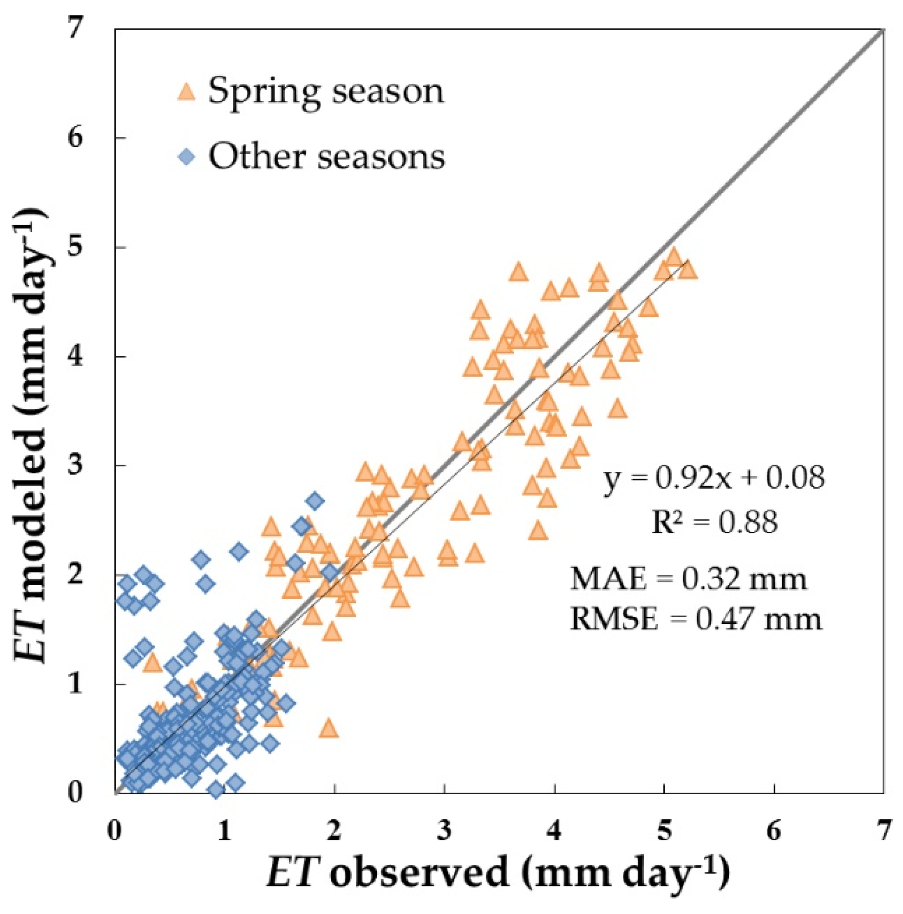
3.1. Parametrization of the VI-ETo Model over the Dehesa Ecosystem and Open Grassland

The application of the VI-ETo model to the study site has combined measured and estimated soil and vegetation parameters. Regarding the soil, the observed physical properties and the computed vegetation root depth resulted in a total amount of water being available for evaporation in the root zone of 283 mm, a value similar to the 280 mm zone computed by Campos et al. [33] for the same landscape. For the vegetation, the calibrated model parameters were K_cb for full cover vegetation, K_{cb full}, and the depletion fraction, p. As can be observed in Figure 2, the sensitivity of the model to the depletion factor is very low in both the whole system and the open grassland components, providing very similar results in the range of 0.4–0.6. Allen et al. [21] discussed the variability of the fraction p as a function of the evaporation power of the atmosphere and the soil type. However, a constant value of p = 0.5 is commonly used for a wide variety of crops, rather than a daily variation. Attending to the results (Figure 2), p was chosen to be equal to 0.5 here for the two situations studied. This value was higher than the 0.3 selected by Campos et al. [33] in the same type of ecosystem. However, different soil or evaporative conditions could contribute to this difference, which as can be derived from Figure 2, has a limited impact on the final ET estimations.

On the other hand, the selection of K_{cb full} = 1 for the whole system resulted in a reduction in RMSE of 0.2 mm when compared with the minimum value considered (K_{cb full} = 0.7). Therefore, the values of the parameters selected for the model application were K_{cb full} = 1 and p = 0.5 (with RMSE = 0.47 mm day⁻¹). In open grassland modeling (Figure 2b), the simulation of increasing K_{cb full} seemed to improve the final RMSE, until it reached a minimum of around K_{cb full} = 1.1, corresponding to the tabulated value of annual herbaceous crops used in previous works [21,52,73]. These results are consistent with the results for the combined dehesa system and the tabulated values for other Mediterranean tree crops (e.g., olive trees) that have similarities with oak trees. The consideration of a K_{cb full} value equal to 1 for the whole system and to 1.1 for grassland implies that K_{cb full} for oak trees might be around 0.7, which is a reasonable value considering that it is similar to the values recommended by some authors for other Mediterranean tree species [21,36]. The selected values of the parameters for model application over grassland, producing a RMSE = 0.47 mm day⁻¹, were K_{cb full} = 1.1 and p = 0.5.

3.2. Dead Grass Impact on ET Estimations during the Dry Season

Figure 3 presents the measured spectral signatures of green grass, senescent grass, and bare soil, with the red and near-infrared regions used to compute NDVI and SAVI highlighted in dark and light pink, respectively. One can observe the low separability of the bare soil and non-photosynthetic grass in the VIS–NIR region [55], as well as the differences in the shortwave infrared region (2.0–2.2 μm), which can be useful for distinguishing both covers.

The field measurements resulted in NDVI and SAVI values of 0.24 and 0.19, respectively, for dead grass, which were significantly higher than values commonly used for soils, with SAVI in the range of 0.08–0.09 and NDVI of 0.1–0.14 [31]. Xu et al. [38] obtained an NDVI of about 0.12 from a simulated relationship between the index and the dead cover, while the NDVI determined by Nagler et al. [57] ranged between 0.25 and 0.3 for dry and wet forest litter, respectively, which was more similar to the values measured in this study. Summer SAVI values derived from the satellite data over the footprint of the open grassland tower when only dead grass is present are always higher than the selected value for soil, which is equal to 0.09, confirming the contribution of dead grass cover to the SAVI values used to estimate f_c.

In the final classification map of land cover on Santa Clotilde farm (Figure 4a), 96.6% of the validation points were classified correctly. The highest mismatches were found in mixed tree and shadow pixels and pure shadows. The classification map obtained for the 1 × 1 km area surrounding the installation (Figure 4c) showed 75% background area (bare soil or non-photosynthetic grass, f_{c grass+soil}) and 25% tree fractional cover (f_{c tree}), similar to the fractional cover computed by Andreu et al. [43]. Considering only the tower footprint area used to compute the whole system VIs, f_{c grass} was equal to 78.5% and f_{c tree} equal to 21.5%. The tree fractional cover on the pasture lower tower footprint was confirmed to be equal to 0%, as originally designed.

The average estimation of the oak tree fractional cover of the ecosystem tower footprint area using satellite-derived SAVI values of the end of the summer (August) and all the years studied yielded a value of f_{c tree} = 24%. The specific value corresponding to 28 August 2015 (when the reference flight was conducted) was equal to 23%. Both values are slightly higher than the 21.5% tree fractional cover computed with the reference classification method. Over the open grassland tower footprint, satellite-estimated summer f_{c tree} was always >0%.

The difference of 1.5% in f_c suggests a certain influence of the dead grass on the satellite VI. However, its size does not seem large enough to justify the use of more precise spectral mixing models or higher complexity algorithms. The accuracy analysis presented in Section 3.3 was also used to support this decision.

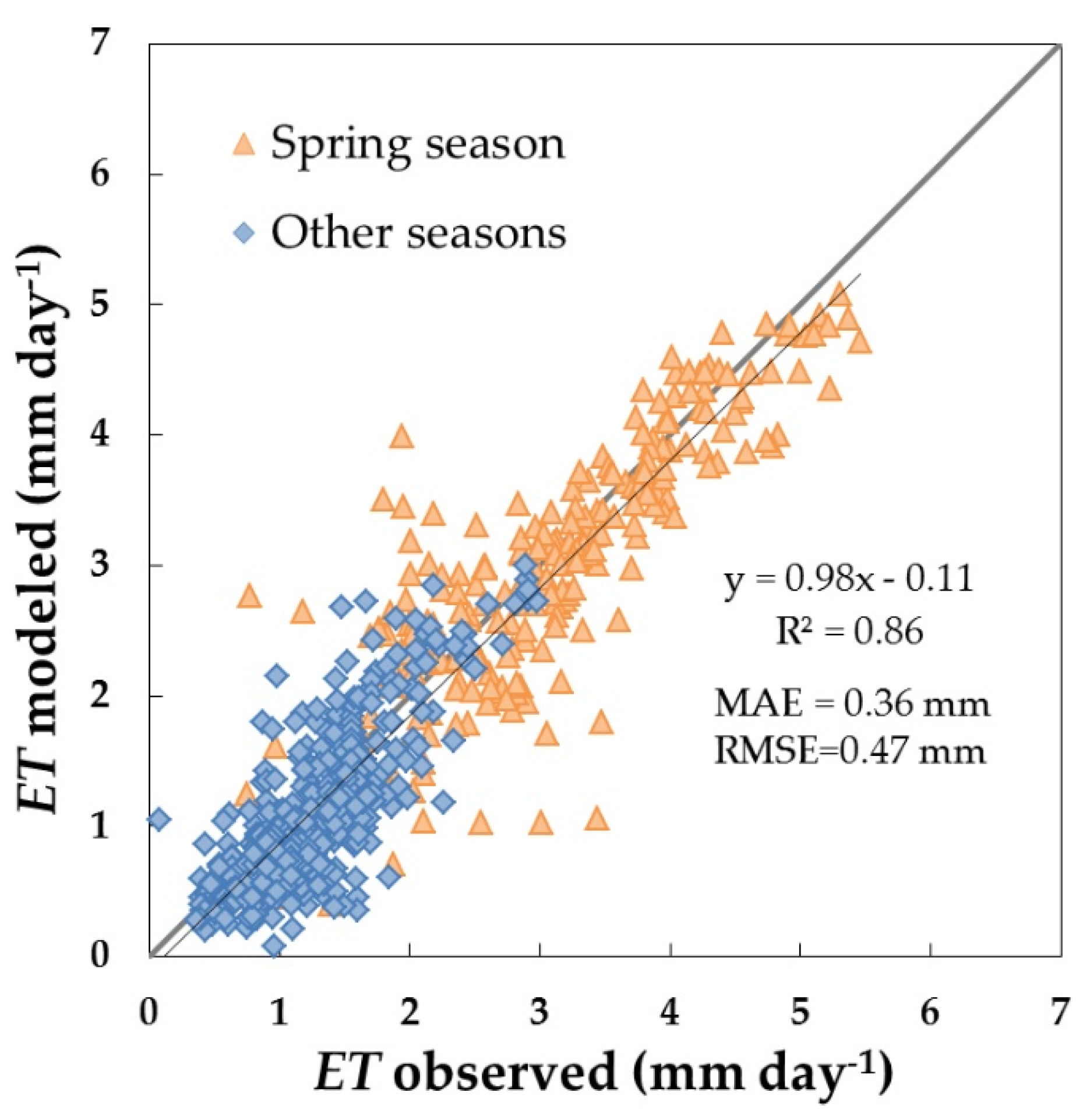
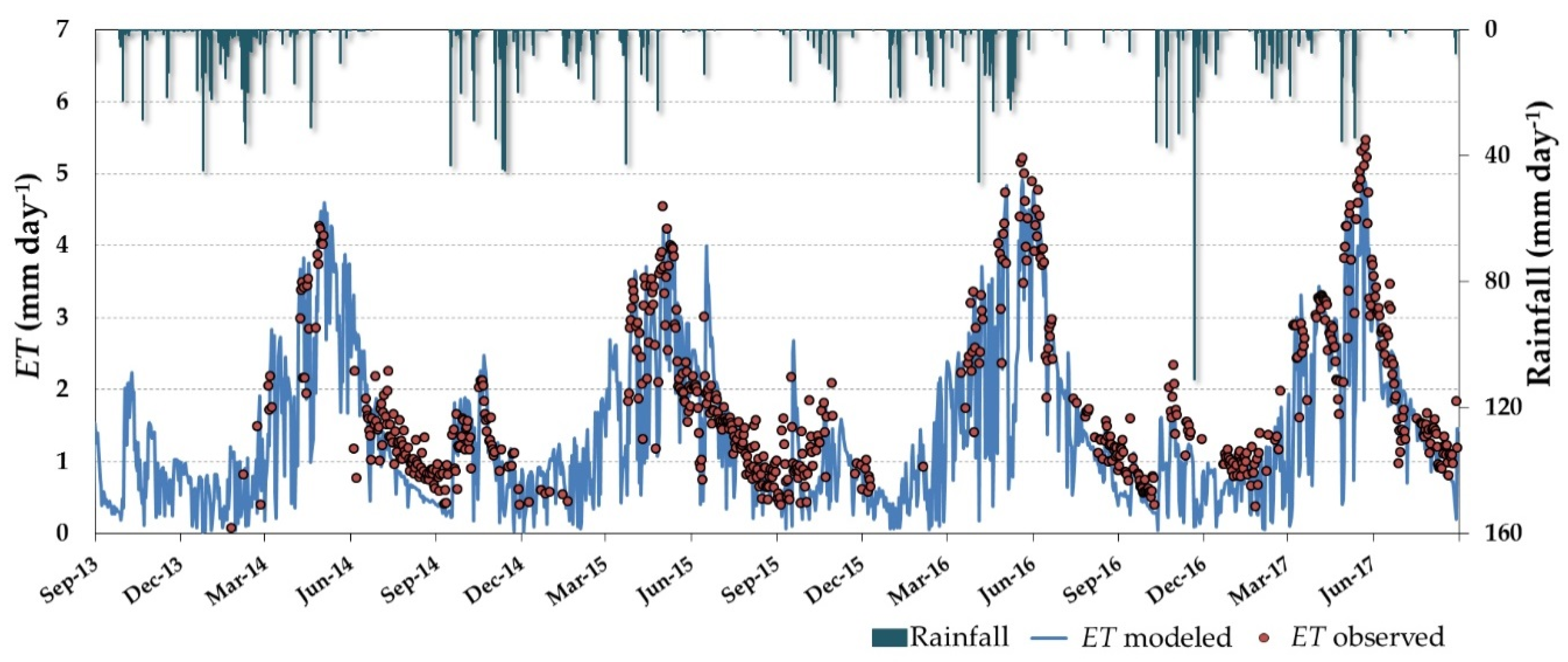
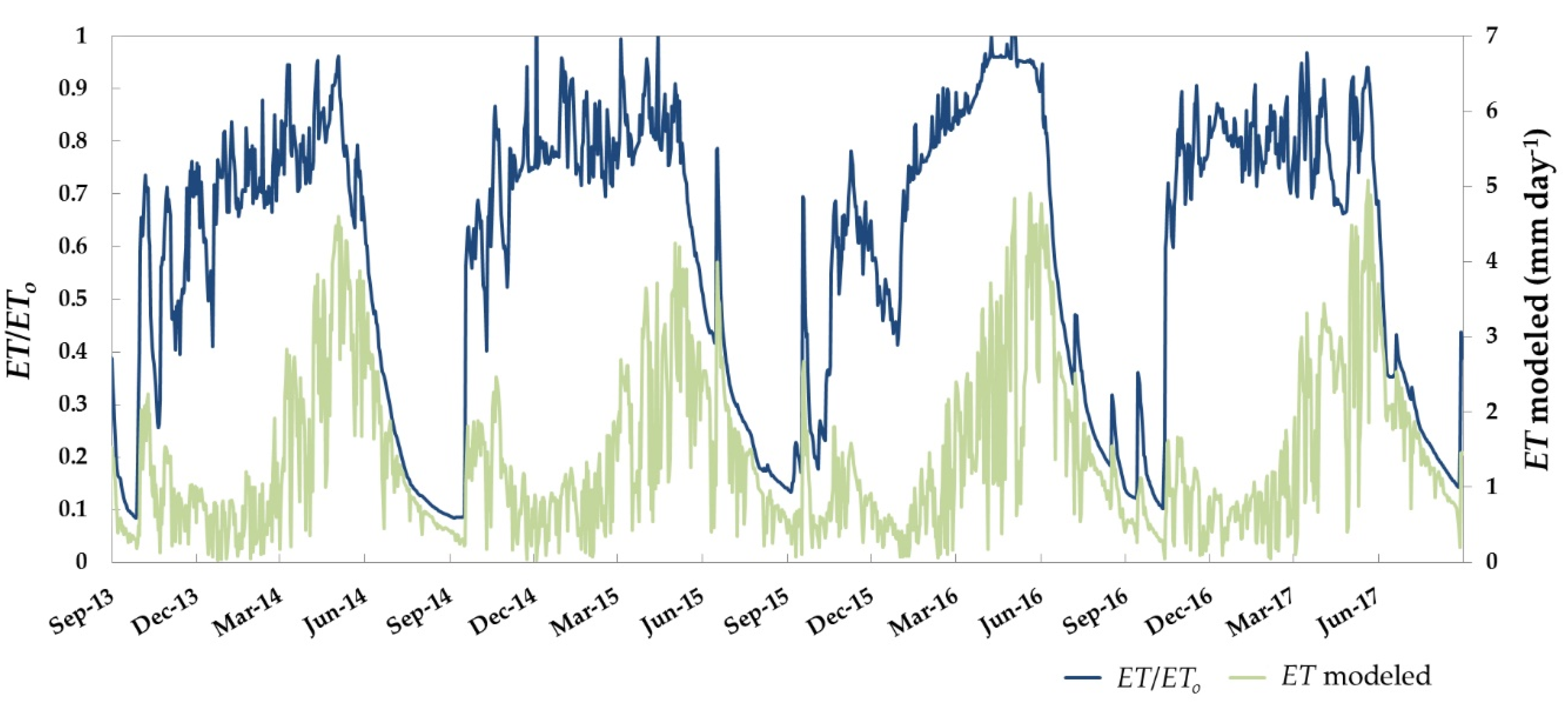
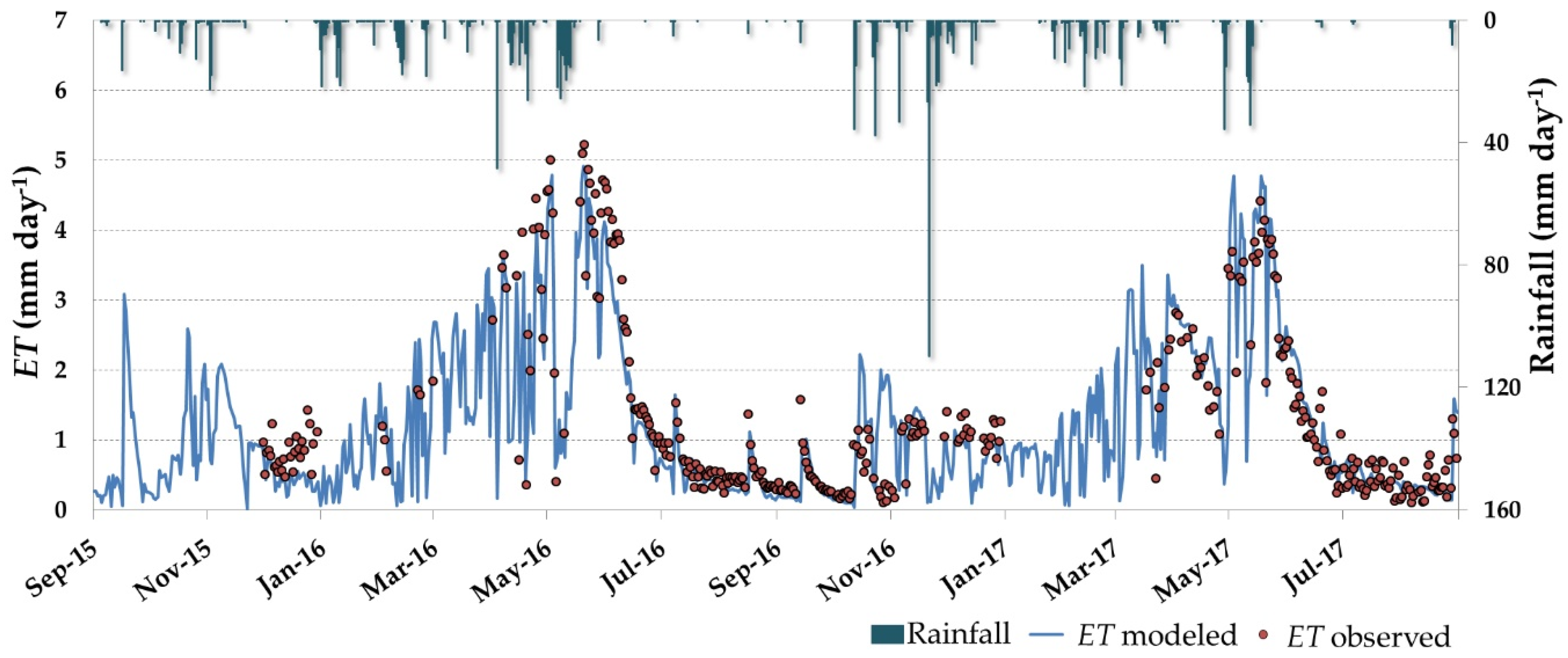
3.3. Daily ET and Water Stress Monitoring over the Dehesa Ecosystem (Tree + Grass)

The modeled daily evapotranspiration is in reasonable agreement with the tower observations for the four hydrological years of the study (2013–2014 to 2016–2017; Figure 5), yielding an RMSE of 0.47 mm day⁻¹ and a relatively low bias of −0.15 mm day⁻¹. This deviation is consistent with previous studies using the VI-ETo FAO-56 dual crop coefficient method in similar ecosystems [33,34] for woody, sparse, semi-arid crops [27,74,75] and for field crops [36,73,76]. Despite the low bias, a slight underestimation of the ET rates can be observed, with a greater impact on the highest ET rates (>4 mm) in spring and a higher dispersion during this season. This underestimation might have an influence on the seasonal or annual computations of water consumption by the system. As an example, during the hydrological year 2016–2017, average weekly ET underestimation changed from 1.8 mm week⁻¹ on average to values of around 5–7 mm week⁻¹ for the springtime (between mid-May and mid-June 2017), decreasing again to 1.6 mm week⁻¹ for the summer. The observed underestimation might be caused by a slight overestimation of some canopy parameters limiting the estimations (SAVI_max, f_c,full). The selection of representative values, accounting for the inter- and intra-annual variability and the behavior of the two vegetation layers, is a challenge, especially if ones wishes to avoid increasing the model’s complexity, which could hinder the final operative applications. Adaptations to account for the major phenological periods were applied over savanna systems to estimate ET using a surface energy balance model [77], which had a high sensitivity to f_c and to parameters related to the vegetation structure. Nevertheless, a daily error of 0.47 mm day⁻¹ can be considered to be admissible to support management actions in the dehesa, with the precision reaching the accuracy requirements for agriculture and water management applications.

Figure 6 shows a daily time step ET series generated for the four hydrological years analyzed (between 2013–2014 and 2016–2017) by the VI-ETo approach, together with ET measurements acquired by the dehesa ECT system and the rainfall data for the period. It can be seen that ET rates present an annual bimodal behavior, with two clear peaks of different sizes. The largest one occurs during the spring, reaching maximum values of around 4–4.5 mm day⁻¹ in the first two years and higher ones of around 5 mm day⁻¹ in the following years. A second smaller peak with maximum values of around 2 mm day⁻¹ appears in the fall. This pattern is closely linked to the distribution of the annual rainfall and is also influenced by variables controlling the availability of energy for the evaporation. Although the average annual rainfall was similar in the first 3 years (653, 633, and 623 mm, respectively) with a wetter final year (731 mm), rainfall distribution is irregular throughout the seasons. The rainiest springs corresponded to the last 2 years (292 and 160 mm, respectively), which were followed by the ET rates, reaching their maxima during the spring of 2016 and the spring of 2017. During the long dry summers, the transpiration of the system was low (1.5 mm on average for the months of July and August) and minima of around 0.5–0.6 mm day⁻¹ were measured at the end of the season (normally in early September before the first rainfall). ET rates during the summer, when the grass was dry and the oak trees transpired at a very low rate, showed the tolerance of this species to water stress. Oak tree roots explore extensive and deep volumes of soil, reaching the groundwater, in addition to forming both arbuscular and ectotrophic mycorrhizae accessing many different resources [7,78]. The ET rates estimated here were lower but in the same range as values presented by David et al. [4], who found that oak trees maintained transpiration rates of above 0.7 mm day⁻¹ during the summer drought.

Figure 6 shows that modeled ET accurately reproduced the temporal dynamics of the water consumed by the dehesa vegetation measured by the flux tower. Due to rainfall events (e.g., July 2015, October 2015, November 2016), isolated ET peaks measured by the ECT were reproduced precisely by the estimations. The temporal resolution of the satellite images was key to mimicking the fast ET pulses in those events and preventing a loss of information. Accounting for intense, short-term events is important for the total annual budgets and for understanding the system’s functioning, and it highlights the value of high temporal resolution satellite data.

The ratio of ET to reference ET (ET/ET_o) at a daily time step for the period 2013–2017 is presented in Figure 7. This index ranges from ~1 when the actual ET covers the atmospheric evaporative demand to approximately 0 as the water deficit develops and the evaporation is close to zero. In this location, ET/ET_o abruptly decreased from the end of May or beginning of June, depending on the year, with a slope of ~−1.5% for all years. The ecosystem’s “dry peak” (ET/ET_o = 0.11) is found at the end of the summer, after a long season without rain. With the first rainfall, this ratio increased until reaching the annual maxima in around May. The falls and winters were noisy and highly influenced by the rainfall, but ET/ET_o varied at values of around >0.6, which can be considered to be the threshold of vegetation water stress. At the end of 2015, there was a small valley in the ET/ET_o values, representing a short period when the vegetation suffered a mild water stress at an unusual time of year. The later recovery from that situation was slower, with growing but lower values than other years, even if ET/ET_o reached the same maximum values afterwards. The results suggest the potential capability of this index as a monitoring tool for assessing anomalous dry periods and events, which can be used to guide management actions leading to maintaining the ecosystem’s stability, both environmentally and economically.

3.4. Estimation of Evapotranspiration of Grass in Open Areas

The RMSE of the estimation of the daily evapotranspiration of grass for the hydrological years 2015–2016 and 2016–2017 was equal to 0.47 mm day⁻¹ when compared with tower measurements (Figure 8). This error is equal to the one obtained over the whole system and consistent with other studies using the VI-ET_o approach in field crops [36,52,73]. A bias of −0.03 mm day⁻¹ was found, which was lower than that for the whole system and with a greater complexity. A clear deviation is found in a number of points, with ET modeled at around ~2 mm day⁻¹ but measured at close to zero mm day⁻¹. These points corresponded to a period during the month of November 2016 (Figure 9), coinciding with some rainfall events. In this case, the modeled data seemed to be better aligned with the previous and following ET rates, and the effect of rainfall water on the instruments could have produced noisy measurements, which were difficult to correct with the automatic data processing.

Figure 9 shows the daily time step ET series for the open grassland estimated for the two hydrological years analyzed (2015–2016 to 2016–2017), together with ET measurements at the open grass tower and rainfall data. The different phenology of the grasses in comparison with the combined system can be observed in Figure 9, with lower rates shown for the dry season, when the grass is dry and the trees are still transpiring. As for the whole tree–grass system, a bimodal shape was also clear for 2015. However, the peak in the fall was not observed in 2016. ET rates reached the maximum values during spring (~5mm day⁻¹, similar to the maxima for the whole ecosystem), sharply decreasing with the drying of the grass, with both maximum values and the ET decreasing process being accurately reproduced by the model, especially in 2017, while in 2016 a slight underestimation can be observed.

Several short-time phenomena measured during this period were also accurately reproduced by the model. In this sense, it is worth mentioning a sharp reduction in the vegetation transpiration in May 2016 as a consequence of an unusually long rainfall event, which was well reproduced by the estimations. It is also possible to observe that the model captured the impact on ET of small isolated rain events, which increased the evaporation rates during the summer of 2016 when the grass fractional cover was close to zero. The identification of the starting dates of grass greening and drying, and the date when the grass layer reached ET maximum rates, which can be derived from the ET series, are key points for management purposes that may help to decide on the livestock grazing period in each field without compromising the conservation of the ecosystem. As mentioned for the system, the importance of the temporal resolution of the remote sensors in the monitoring of this vegetation layer is noted here, where the drying process usually occurs in a few days as a function of the fast depletion of soil water content and increasing evaporative demand. Information on the system’s functioning could be lost with a lower frequency of available images, which at this time of the year can also be affected by cloudiness. The temporal resolution of Sentinel-2 was found to be well suited for this application.

ET basal rates (0.3–0.4) were maintained during the dry season, where no rainfall was observed and the grass was mostly dry. This could be explained by the presence of morning dew and humidity condensing in the dry grass pockets and later evaporating, with a small percentage being due to the metabolism of heterotrophs and dead grass becoming converted into organic matter by microorganisms [79,80]. In addition, a scattering of photosynthetically active plants were still found throughout the summer. Small gramineae individuals even survived in August, as they were protected by dry grass cover, but the most abundant species was Senecio jacobaea L., a tap-rooted compositae that explores deeper soil profiles.

The comparison of the estimated stress coefficient K_s and the soil water content is presented in Figure 10. It can be seen that the K_s curve is, in general, consistent with the evolution of the water content. When the soil moisture reached a threshold equal to field capacity, the K_s took and maintained the maximum value. Values of soil water content below 0.15 cm³ cm⁻³, in agreement with Gómez-Giráldez et al. [81], generally marked the starting of K_s reduction.

4. Conclusions

The VI-ETo model accurately reproduced the temporal dynamics of daily water consumption of a dehesa ecosystem measured by an eddy covariance flux tower over four years. The results yielded an RMSE value of 0.47 mm day⁻¹ and a low bias (−0.15 m mday⁻¹), similar to the errors presented in the literature for more homogeneous systems using similar approaches. Moreover, a separate application in an open grassland—the predominant component in the occupied area—produced similar results, with an RMSE of 0.47 mm day⁻¹ and a bias of −0.03 mm day⁻¹ for the two years analyzed. This work has provided effective parameters for applying a remote sensing-based water balance method over an oak-–grass savanna, in addition to analyzing each of its components. Reasonable parameters for one component of the system, the grass, were proposed and tested, while suggested values for the oak trees are yet to be validated. This proposal opens up new insights into the high diversity in water use of different grassland communities in the dehesa, the role of oak trees in the hydrology of the systems, and the potential impact of the possible reduction in water availability in the future.

The ET of the system presented an annual bimodal behavior, with two clear peaks of different sizes in spring (ET of 4.5–5 mm day⁻¹) and fall (ET around 2 mm day⁻¹). This pattern was repeated for all the years studied and could be closely linked to the distribution of the annual rainfall. The water stress of the whole system and the grassland was monitored using the ET/ET_o ratio. This index helped to identify periods of water stress, which were confirmed for the grassland by the soil water content measured.

The temporal resolution of the satellite images and the modeling scheme allowed the reproduction of fast and isolated ET pulses that are important for computing accurate annual budgets and for understanding the hydrologic behavior of the system. The identification of the starting dates of grass greening and drying, as well as the date when the grass reaches maximum ET rates, could be useful for management and conservation purposes, such as making decisions on the livestock grazing period in every field. Thus, the temporal resolution of Sentinel-2 was found to be well suited for the monitoring of these processes.

The effect of the non-photosynthetic grass layer on f_c estimation was evaluated using field measurements, airborne data, and satellite data. A slight deviation in tree f_c estimation (1.5 %) using summer satellite VIs was corroborated, although it was not considered large enough to justify the use of more precise spectral mixing models or higher complexity algorithms.

References

1. Birot, Y.; Gracia, C.; Palahí, M. Water for Forests and People in the Mediterranean: A Challenging Balance. What Science Can Tell Us; European Forest Institute: Helsinki, Finland, 2011; ISBN 9789525453799. [Google Scholar]
2. Milano, M.; Ruelland, D.; Fernandez, S.; Dezetter, A.; Fabre, J.; Servat, E.; Fritsch, J.M.; Ardoin-Bardin, S.; Thivet, G. Current state of Mediterranean water resources and future trends under climatic and anthropogenic changes. Hydrol. Sci. J. 2013, 58, 498–518. [Google Scholar] [CrossRef]
3. Baldocchi, D.D.; Xu, L. What limits evaporation from Mediterranean oak woodlands—The supply of moisture in the soil, physiological control by plants or the demand by the atmosphere? Adv. Water Resour. 2007, 30, 2113–2122. [Google Scholar] [CrossRef]
4. David, T.S.; Henriques, M.O.; Kurz-Besson, C.; Nunes, J.; Valente, F.; Vaz, M.; Pereira, J.S.; Siegwolf, R.; Chaves, M.M.; Gazarini, L.C.; et al. Water-use strategies in two co-occurring Mediterranean evergreen oaks: Surviving the summer drought. Tree Physiol. 2007, 27, 793–803. [Google Scholar] [CrossRef] [PubMed] [Green Version]
5. Moreno, G.; Pulido, F.J. The Functioning, Management and Persistence of Dehesas. Agrofor. Eur. 2008, 10600, 127–160. [Google Scholar] [CrossRef]
6. Moreno, G.; Obrador, J.J.; Cubera, E.; Dupraz, C. Fine root distribution in Dehesas of Central-Western Spain. Plant Soil 2005, 277, 153–162. [Google Scholar] [CrossRef]
7. Cubera, E.; Morena, G. Effect of single Quercus ilex trees upon spatial and seasonal changes in soil water content in dehesas of central western Spain. Ann. For. Sci. 2007, 64, 355–364. [Google Scholar] [CrossRef] [Green Version]
8. Joffre, R.; Rambal, S. How tree cover influences the water balance of Mediterranean rangelands. Ecology 1993, 74, 570–582. [Google Scholar] [CrossRef]
9. Gauquelin, T.; Michon, G.; Joffre, R.; Duponnois, R.; Génin, D.; Fady, B.; Bou Dagher-Kharrat, M.; Derridj, A.; Slimani, S.; Badri, W.; et al. Mediterranean forests, land use and climate change: A social-ecological perspective. Reg. Environ. Chang. 2018, 18, 623–636. [Google Scholar] [CrossRef]
10. Campos, P.; Huntsinger, L.; Oviedo, J.; Díaz, M.; Starrs, P.; Standiford, R.; Montero, G. Mediterranean Oak Woodland Working Landscapes: Dehesas of Spain and Ranchlands of California; Springer: Berlin, Germany, 2013; ISBN 978-94-007-6706-5. [Google Scholar]
11. Plieninger, T.; Rolo, V.; Moreno, G. Large-scale patterns of Quercus ilex, Quercus suber, and Quercus pyrenaica regeneration in central-western Spain. Ecosystems 2010, 13, 644–660. [Google Scholar] [CrossRef]
12. Coelho, C.; Ferreira, A.J.D.; Laouina, A.; Hamza, A.; Chaker, M.; Naafa, R.; Regaya, K.; Boulet, A.-K.; Keizer, J.J.; Carvalho, T.M.M. Changes in Land Use and Land Management Practices Affecting Land Degradation within Forest and Grazing Ecosystems in the Western Mediterranean. In Sustainability of Agrosylvopastoral Systems, Dehesas, Montados; Schnabel, S., Ferreira, A., Eds.; Schweizerbart Science Publishers: Stuttgart, Germany, 2004; pp. 137–154. ISBN 978-3-923381-50-0. [Google Scholar]
13. Giorgi, F.; Lionello, P. Climate change projections for the Mediterranean region. Glob. Planet. Chang. 2008, 63, 90–104. [Google Scholar] [CrossRef]
14. Jacob, D.; Petersen, J.; Eggert, B.; Alias, A.; Christensen, O.B.; Bouwer, L.M.; Braun, A.; Colette, A.; Déqué, M.; Georgievski, G.; et al. EURO-CORDEX: New high-resolution climate change projections for European impact research. Reg. Environ. Chang. 2014, 14, 563–578. [Google Scholar] [CrossRef]
15. Mishra, A.K.; Singh, V.P. A review of drought concepts. J. Hydrol. 2010, 391, 202–216. [Google Scholar] [CrossRef]
16. Milano, M.; Ruelland, D.; Fernandez, S.; Dezetter, A.; Ardoin-Bardin, S.; Fabre, J.; Thivet, G.; Servat, E. Assessing the impacts of global changes on the water resources of the Mediterranean basin. IAHS AISH Publ. 2011, 347, 165–172. [Google Scholar]
17. Polade, S.D.; Pierce, D.W.; Cayan, D.R.; Gershunov, A.; Dettinger, M.D. The key role of dry days in changing regional climate and precipitation regimes. Sci. Rep. 2014, 4. [Google Scholar] [CrossRef] [Green Version]
18. Schleussner, C.F.; Lissner, T.K.; Fischer, E.M.; Wohland, J.; Perrette, M.; Golly, A.; Rogelj, J.; Childers, K.; Schewe, J.; Frieler, K.; et al. Differential climate impacts for policy-relevant limits to global warming: The case of 1.5 °C and 2 °C. Earth Syst. Dyn. 2016, 7, 327–351. [Google Scholar] [CrossRef] [Green Version]
19. García-Ruiz, J.M.; López-Moreno, I.I.; Vicente-Serrano, S.M.; Lasanta-Martínez, T.; Beguería, S. Mediterranean water resources in a global change scenario. Earth Sci. Rev. 2011, 105, 121–139. [Google Scholar] [CrossRef] [Green Version]
20. Seneviratne, S.I.; Wartenburger, R.; Guillod, B.P.; Hirsch, A.L.; Vogel, M.M.; Brovkin, V.; Van Vuuren, D.P.; Schaller, N.; Boysen, L.; Calvin, K.V.; et al. Climate extremes, land-climate feedbacks and land-use forcing at 1.5°C. Philos. Trans. R. Soc. A Math. Phys. Eng. Sci. 2018, 376. [Google Scholar] [CrossRef]
21. Allen, R.G.; Pereira, L.S.; Raes, D.; Smith, M. Crop Evapotranspiration-Guidelines for Computing Crop Water Requirements-FAO; Irrigation and Drainage Paper 56; FAO: Rome, Italy, 1998; Available online: http://www.fao.org/3/x0490e/x0490e00.htm (accessed on 27 November 2019).
22. Allen, R.G.; Pereira, L.S.; Smith, M.; Raes, D.; Wright, J.L. FAO-56 dual crop coefficient method for estimating evaporation from soil and application extensions. J. Irrig. Drain. Eng. 2005, 131, 2–13. [Google Scholar] [CrossRef] [Green Version]
23. Bausch, W.C. Remote sensing of crop coefficients for improving the irrigation scheduling of corn. Agric. Water Manag. 1995, 27, 55–68. [Google Scholar] [CrossRef]
24. Jayanthi, H.; Neale, C.M.U. Seasonal evapotranspiration estimation using canopy reflectance: A case study involving pink beans. IAHS AISH Publ. 2001, 2000, 302–305. [Google Scholar]
25. Er-Raki, S.; Chehbouni, A.; Guemouria, N.; Duchemin, B.; Ezzahar, J.; Hadria, R. Combining FAO-56 model and ground-based remote sensing to estimate water consumptions of wheat crops in a semi-arid region. Agric. Water Manag. 2007, 87, 41–54. [Google Scholar] [CrossRef] [Green Version]
26. González-Dugo, M.P.; Mateos, L. Spectral vegetation indices for benchmarking water productivity of irrigated cotton and sugarbeet crops. Agric. Water Manag. 2008, 95, 48–58. [Google Scholar] [CrossRef]
27. Consoli, S.; Vanella, D. Mapping crop evapotranspiration by integrating vegetation indices into a soil water balance model. Agric. Water Manag. 2014, 143, 71–81. [Google Scholar] [CrossRef]
28. Odi-Lara, M.; Campos, I.; Neale, C.M.U.; Ortega-Farías, S.; Poblete-Echeverría, C.; Balbontín, C.; Calera, A. Estimating evapotranspiration of an apple orchard using a remote sensing-based soil water balance. Remote Sens. 2016, 8, 253. [Google Scholar] [CrossRef] [Green Version]
29. Glenn, E.P.; Neale, C.M.U.; Hunsaker, D.J.; Nagler, P.L. Vegetation index-based crop coefficients to estimate evapotranspiration by remote sensing in agricultural and natural ecosystems. Hydrol. Process. 2011, 25, 4050–4062. [Google Scholar] [CrossRef]
30. Calera, A.; Campos, I.; Osann, A.; D’Urso, G.; Menenti, M. Remote sensing for crop water management: From ET modelling to services for the end users. Sensors 2017, 17, 1104. [Google Scholar] [CrossRef] [Green Version]
31. Pôças, I.; Calera, A.; Campos, I.; Cunha, M. Remote sensing for estimating and mapping single and basal crop coefficientes: A review on spectral vegetation indices approaches. Agric. Water Manag. 2020, 233, 106081. [Google Scholar] [CrossRef]
32. Glenn, E.P.; Nagler, P.L.; Huete, A.R. Vegetation Index Methods for Estimating Evapotranspiration by Remote Sensing. Surv. Geophys. 2010, 31, 531–555. [Google Scholar] [CrossRef]
33. Campos, I.; Villodre, J.; Carrara, A.; Calera, A. Remote sensing-based soil water balance to estimate Mediterranean holm oak savanna (dehesa) evapotranspiration under water stress conditions. J. Hydrol. 2013, 494, 1–9. [Google Scholar] [CrossRef]
34. Andreu, A.; Dube, T.; Nieto, H.; Mudau, A.E.; González-Dugo, M.P.; Guzinski, R.; Hülsmann, S. Remote sensing of water use and water stress in the African savanna ecosystem at local scale – Development and validation of a monitoring tool. Phys. Chem. Earth 2019, 112, 154–164. [Google Scholar] [CrossRef]
35. Carpintero, E.; Mateos, L.; Andreu, A.; González-Dugo, M.P. Effect of the differences in spectral response of Mediterranean tree canopies on the estimation of evapotranspiration using vegetation index-based crop coefficients. Agric. Water Manag. 2020, 238, 106–201. [Google Scholar] [CrossRef]
36. Mateos, L.; González-Dugo, M.P.; Testi, L.; Villalobos, F.J. Monitoring evapotranspiration of irrigated crops using crop coefficients derived from time series of satellite images. I. Method validation. Agric. Water Manag. 2013, 125, 81–91. [Google Scholar] [CrossRef]
37. Roberts, D.A.; Smith, M.O.; Adams, J.B. Green vegetation, nonphotosynthetic vegetation, and soils in AVIRIS data. Remote Sens. Environ. 1993, 44, 255–269. [Google Scholar] [CrossRef]
38. Xu, D.; Guo, X.; Li, Z.; Yang, X.; Yin, H. Measuring the dead component of mixed grassland with Landsat imagery. Remote Sens. Environ. 2014, 142, 33–43. [Google Scholar] [CrossRef]
39. Rivas Martínez, S. Bioclimatología, biogeografía y series de vegetación de Andalucía Occidental. Lagascalia 1988, 15, 91–120. [Google Scholar]
40. Melendo, M. Cartografía y Ordenación Vegetal de Sierra Morena: Parque Natural de Las Sierras de Cardeña y Montoro; Universidad de Jaén: Jaén, Spain, 1998. [Google Scholar]
41. Román-Sánchez, A.; Vanwalleghem, T.; Peña, A.; Laguna, A.; Giráldez, J.V. Controls on soil carbon storage from topography and vegetation in a rocky, semi-arid landscapes. Geoderma 2018, 311, 159–166. [Google Scholar] [CrossRef]
42. Webb, E.K.; Pearman, G.I.; Leuning, R. Correction of flux measurements for density effects due to heat and water vapour transfer. Q. J. R. Meteorol. Soc. 1980, 106, 85–100. [Google Scholar] [CrossRef]
43. Andreu, A.; Kustas, W.P.; Polo, M.J.; Carrara, A.; González-Dugo, M.P. Modeling surface energy fluxes over a dehesa (oak savanna) ecosystem using a thermal based two-source energy balance model (TSEB) I. Remote Sens. 2018, 10, 567. [Google Scholar] [CrossRef] [Green Version]
44. Mauder, M.; Genzel, S.; Fu, J.; Kiese, R.; Soltani, M.; Steinbrecher, R.; Zeeman, M.; Banerjee, T.; De Roo, F.; Kunstmann, H. Evaluation of energy balance closure adjustment methods by independent evapotranspiration estimates from lysimeters and hydrological simulations. Hydrol. Process. 2018, 32, 39–50. [Google Scholar] [CrossRef]
45. Hsieh, C.I.; Katul, G.; Chi, T.W. An approximate analytical model for footprint estimation of scalar fluxes in thermally stratified atmospheric flows. Adv. Water Resour. 2000, 23, 765–772. [Google Scholar] [CrossRef]
46. Wright, J.L. New Evapotranspiration Crop Coefficients. J. Irrig. Drain. Div. ASCE 1982, 108, 57–74. [Google Scholar]
47. Hunsaker, D.J.; Pinter, P.J.; Barnes, E.M.; Kimball, B.A. Estimating cotton evapotranspiration crop coefficients with a multispectral vegetation index. Irrig. Sci. 2003, 22, 95–104. [Google Scholar] [CrossRef]
48. Gonzalez-Piqueras, J.; Calera, A.; Gilabert, M.A.; Cuesta, A.; De la Cruz Tercero, F. Estimation of crop coefficients by means of optimized vegetation indices for corn. Remote Sens. Agric. Ecosyst. Hydrol. V 2004, 5232, 110. [Google Scholar] [CrossRef]
49. Hunsaker, D.J.; Pinter, P.J.; Kimball, B.A. Wheat basal crop coefficients determined by normalized difference vegetation index. Irrig. Sci. 2005, 24, 1–14. [Google Scholar] [CrossRef]
50. Jayanthi, H.; Neale, C.M.U.; Wright, J.L. Development and validation of canopy reflectance-based crop coefficient for potato. Agric. Water Manag. 2007, 88, 235–246. [Google Scholar] [CrossRef]
51. Campos, I.; Neale, C.M.U.; Calera, A.; Balbontín, C.; González-Piqueras, J. Assessing satellite-based basal crop coefficients for irrigated grapes (Vitis vinifera L.). Agric. Water Manag. 2010, 98, 45–54. [Google Scholar] [CrossRef]
52. Gonzalez-Dugo, M.P.; Neale, C.M.U.; Mateos, L.; Kustas, W.P.; Prueger, J.H.; Anderson, M.C.; Li, F. A comparison of operational remote sensing-based models for estimating crop evapotranspiration. Agric. For. Meteorol. 2009, 149, 1843–1853. [Google Scholar] [CrossRef]
53. Huete, A.R. A soil-adjusted vegetation index (SAVI). Remote Sens. Environ. 1988, 25, 295–309. [Google Scholar] [CrossRef]
54. Anderson, M.C.; Zolin, C.A.; Sentelhas, P.C.; Hain, C.R.; Semmens, K.; Tugrul Yilmaz, M.; Gao, F.; Otkin, J.A.; Tetrault, R. The Evaporative Stress Index as an indicator of agricultural drought in Brazil: An assessment based on crop yield impacts. Remote Sens. Environ. 2016, 174, 82–99. [Google Scholar] [CrossRef]
55. Nagler, P.L.; Inoue, Y.; Glenn, E.P.; Russ, A.L.; Daughtry, C.S.T. Cellulose absorption index (CAI) to quantify mixed soil-plant litter scenes. Remote Sens. Environ. 2003, 87, 310–325. [Google Scholar] [CrossRef]
56. Aase, J.K.; Tanaka, D.L. Reflectances from Four Wheat Residue Cover Densities as Influenced by Three Soil Backgrounds. Agron. J. 1991, 83, 753–757. [Google Scholar] [CrossRef]
57. Nagler, P.L.; Daughtry, C.S.T.; Goward, S.N. Plant litter and soil reflectance. Remote Sens. Environ. 2000, 71, 207–215. [Google Scholar] [CrossRef]
58. Mueller-Wilm, U.; Devignot, O.; Pessiot, L. Sen2Core Configuration and User Manual. Ref. S2-PDGS-MPC-L2A- SUM-V2.3 eesa Sentinel 2. Version: 1 November 2017. Available online: https://step.esa.int/thirdparties/sen2cor/2.4.0/Sen2Cor_240_Documenation_PDF/S2-PDGS-MPC-L2A-SUM-V2.4.0.pdf (accessed on 14 October 2019).
59. Gao, F.; Masek, J.; Schwaller, M.; Hall, F. On the blending of the landsat and MODIS surface reflectance: Predicting daily landsat surface reflectance. IEEE Trans. Geosci. Remote Sens. 2006, 44, 2207–2218. [Google Scholar] [CrossRef]
60. Rodríguez, J.; Sotelo, A.; Monge, G.; De la Rosa, D. Sistema de Inferencia Espacial de Propiedades de Los Suelos de Andalucía; Consejería de Agricultura y Pesca: Sevilla, Spain, 2008. [Google Scholar]
61. Mbah, C.N. Determining the field capacity, wilting point and available water capacity of some Southeast Nigerian soils using soil saturation from capillary rise. Niger. J. Biotechnol. 2012, 24, 41–47. [Google Scholar]
62. Pulido-Fernández, M.; Schnabel, S.; Lavado-Contador, J.F.; Miralles Mellado, I.; Ortega Pérez, R. Soil organic matter of Iberian open woodland rangelands as influenced by vegetation cover and land management. Catena 2013, 109, 13–24. [Google Scholar] [CrossRef]
63. Moreno, G.; Cáceres, Y. System report: Iberian Dehesas, Spain; AGFORWARD; Agroforestry for Europe: Plasencia, Spain, 2016. [Google Scholar]
64. Canadell, J.; Jackson, R.B.; Ehleringer, J.R.; Mooney, H.A.; Sala, O.E.; Schulze, E.D. Maximum rooting depth of vegetation types at the global scale. Oecologia 1996, 108, 583–595. [Google Scholar] [CrossRef] [PubMed]
65. Rolo, V.; López-Díaz, M.L.; Moreno, G. Shrubs affect soil nutrients availability with contrasting consequences for pasture understory and tree overstory production and nutrient status in Mediterranean grazed open woodlands. Nutr. Cycl. Agroecosystems 2012, 93, 89–102. [Google Scholar] [CrossRef]
66. Pierret, A.; Maeght, J.L.; Clément, C.; Montoroi, J.P.; Hartmann, C.; Gonkhamdee, S. Understanding deep roots and their functions in ecosystems: An advocacy for more unconventional research. Ann. Bot. 2016, 118, 621–635. [Google Scholar] [CrossRef] [PubMed] [Green Version]
67. Stegman, E.C.; Musick, J.T.; Stewart, J.I. Irrigation water management. In Design and Operation of Farm Irrigation Systems; American Society of Agricultural Engineers: San Jose, MI, USA, 1980; pp. 763–768. ISBN 0-916150-28-3. [Google Scholar]
68. Browne, M.W. Cross-Validation Methods. J. Math. Psychol. 2000, 44, 108–132. [Google Scholar] [CrossRef] [Green Version]
69. Arlot, S.; Celisse, A. A survey of cross-validation procedures for model selection. Stat. Surv. 2010, 4, 40–79. [Google Scholar] [CrossRef]
70. Lee, G.; Kim, W.; Oh, H.; Youn, B.D.; Kim, N.H. Review of statistical model calibration and validation—from the perspective of uncertainty structures. Struct. Multidiscip. Optim. 2019, 60, 1619–1644. [Google Scholar] [CrossRef]
71. Schoups, G.; Van De Giesen, N.C.; Savenije, H.H.G. Model complexity control for hydrologic prediction. Water Resour. Res. 2008, 44, 1–14. [Google Scholar] [CrossRef] [Green Version]
72. Tegegne, G.; Park, D.K.; Kim, Y.O. Comparison of hydrological models for the assessment of water resources in a data-scarce region, the Upper Blue Nile River Basin. J. Hydrol. Reg. Stud. 2017, 14, 49–66. [Google Scholar] [CrossRef]
73. Padilla, F.L.M.; González-Dugo, M.P.; Gavilán, P.; Domínguez, J. Integration of vegetation indices into a water balance model to estimate evapotranspiration of wheat and corn. Hydrol. Earth Syst. Sci. 2011, 15, 1213–1225. [Google Scholar] [CrossRef] [Green Version]
74. Cammalleri, C.; Ciraolo, G.; Minacapilli, M.; Rallo, G. Evapotranspiration from an Olive Orchard using Remote Sensing-Based Dual Crop Coefficient Approach. Water Resour. Manag. 2013, 27, 4877–4895. [Google Scholar] [CrossRef]
75. Campos, I.; Balbontín, C.; González-Piqueras, J.; González-Dugo, M.P.; Neale, C.M.U.; Calera, A. Combining a water balance model with evapotranspiration measurements to estimate total available soil water in irrigated and rainfed vineyards. Agric. Water Manag. 2016, 165. [Google Scholar] [CrossRef]
76. González-Dugo, M.P.; Escuin, S.; Cano, F.; Cifuentes, V.; Padilla, F.L.M.; Tirado, J.L.; Oyonarte, N.; Fernández, P.; Mateos, L. Monitoring evapotranspiration of irrigated crops using crop coefficients derived from time series of satellite images. II. Application on basin scale. Agric. Water Manag. 2013, 125, 92–104. [Google Scholar] [CrossRef]
77. Burchard-Levine, V.; Nieto, H.; Riaño, D.; Migliavacca, M.; El-Madany, T.S.; Perez-Priego, O.; Carrara, A.; Martín, M.P. Seasonal adaptation of the thermal-based two-source energy balance model for estimating evapotranspiration in a semiarid tree-grass ecosystem. Remote Sens. 2020, 12, 904. [Google Scholar] [CrossRef] [Green Version]
78. Allen, M.F. How Oaks Respond to Water Limitation. In Proceedings of the Seventh California Oak Symposium: Managing Oak Woodlands in a Dynamic World, Albany, CA, USA, 3–6 November 2014; pp. 13–21. [Google Scholar]
79. Xu, L.; Baldocchi, D.D.; Tang, J. How soil moisture, rain pulses, and growth alter the response of ecosystem respiration to temperature. Glob. Biogeochem. Cycles 2004, 18. [Google Scholar] [CrossRef]
80. Fischer, Z.; Blažka, P. Soil Respiration in Drying of an Organic Soil. Open J. Soil Sci. 2015, 5, 181–192. [Google Scholar] [CrossRef] [Green Version]
81. Gómez-Giráldez, P.J.; Pérez-Palazón, M.J.; Polo, M.J.; González-Dugo, M.P. Monitoring grass phenology and hydrological dynamics of an oak-grass savanna ecosystem using sentinel-2 and terrestrial photography. Remote Sens. 2020, 12, 600. [Google Scholar] [CrossRef] [Green Version]
Figure 1. (a) Distribution of the dehesa ecosystem in the Iberian Peninsula (in green) and the study area location (b) Eddy covariance tower (ECT) over open grassland. (c) ECT over the combined tree + grassland system; (d) Aerial photograph showing the locations of validation sites.
Water 12 01418 g001
Figure 2. Performance (Root Mean Square Error, RMSE) of the soil water balance over the (a) dehesa ecosystem and (b) grassland area, with a range of basal crop coefficients for full cover vegetation (Kcb full) (0.7–1.1) and depletion fractions (p) (0.3–0.7) parameters.
Water 12 01418 g002
Figure 3. The spectral response measured with the spectroradiometer of bare soil, along with images of photosynthetic and non-photosynthetic grass under full vegetation conditions.
Water 12 01418 g003
Figure 4. Classification map for the ecosystem eddy covariance tower.
Water 12 01418 g004
Figure 5. Comparison between observed and modeled daily evapotranspiration (ET) values (mm) for the dehesa system (tree + grass) for the four hydrological years analyzed (between 2013–2014 and 2016–2017). Root Mean Square Error (RMSE) and Mean Absolute Error (MAE) are presented in the figure.
Water 12 01418 g005
Figure 6. Daily evapotranspiration (ET) monitoring over the dehesa ecosystem, considering basal crop coefficients for full cover vegetation, Kcb full = 1, and the depletion fraction, p = 0.5. Dark green bars illustrate rainfall events.
Water 12 01418 g006
Figure 7. Daily evapotranspiration (ET) monitoring and water stress (ratio between evapotranspiration and reference evapotranspiration, ET/ETo) over the dehesa ecosystem.
Water 12 01418 g007
Figure 8. Comparison between observed and modeled daily evapotranspiration (ET) values over the grass area (mm) for the hydrological years 2015–2016 and 2016–2017. Root Mean Square Error (RMSE) and Mean Absolute Error (MAE) are presented in the figure.
Water 12 01418 g008
Figure 9. Daily evapotranspiration (ET) monitoring over grassland, considering the basal crop coefficient for full cover vegetation, Kcb full =1.1, and the depletion fraction, p = 0.5. Dark green bars illustrate rainfall events.
Water 12 01418 g009
Figure 10. Daily evolution of water stress coefficient, Ks, computed by the VI-ETo method and soil water content over the open grassland.
Water 12 01418 g010