Experimental Analysis of Velocity Distribution in a Coarse-Grained Debris Flow: A Modified Bagnold’s Equation


1
Department of Engineering, University of Palermo, 90128 Palermo, Italy
2
Faculty of Engineering, University Enna Kore, 94100 Enna, Italy
*
Author to whom correspondence should be addressed.
Water 2020, 12(5), 1415; https://doi.org/10.3390/w12051415
Submission received: 26 February 2020
/
Revised: 8 May 2020
/
Accepted: 11 May 2020
/
Published: 15 May 2020
(This article belongs to the Special Issue Flow Hydrodynamic in Open Channels: Interaction with Natural or Man-Made Structures)
Abstract
:Today, Bagnold’s theory is still applied to gravity-driven flows under the assumption of uniform sediment concentration. This study presents findings of flume experiments conducted to investigate the velocity and concentration distributions within the debris body by using high-resolution images. The analysis has shown that the concentration and mobility of grains vary along the depth. A linear law to interpret the grains concentration distribution, starting from the knowledge of the packing concentration and of the surface concentration, Cs, has been identified. By considering such a law, modified expressions of the Bagnold’s number and the velocity in stony-type debris flows are also presented. By using these expressions, three regimes of motion have been identified along the depth, and the velocity profile within the debris body is determined as a function of the parameter Cs. It has been verified that the velocity profiles estimated by using the modified equation compare well (mean square error less than 0.1) with the literature’s measured profiles when Cs is correctly measured or estimated. Results of cutting tests, conducted for a sample of the used material, have also allowed us to verify that Cs could be determined as a function of the static friction angle of the material.
1. Introduction
Coarse-grained debris flows represent the gravity-driven motion of granular sediment, which especially occurs in steep valleys and rivers [1,2]. These flows consist of rapid movements of mass that might determine forces of high-impact and, consequently, serious hazards, loss of human life, and structural damage.
The identification of laws governing hydrodynamics of flows in steep river reaches is less advanced than in lowland river systems [3]. This is especially related to the fact that different flow behaviors can be obtained, depending on the concentration and composition of sediments. Consequently, a wide range of coarse-grained debris flows, characterized by different internal stress distributions, can be observed [4,5,6]. The sediment transport processes in flows characterized by small sediment concentrations have been largely analyzed, and different approaches to treat the bed load and the suspended load can be found in the literature, among others [7,8,9,10]. In flows characterized by high sediment concentrations, such as in debris flows, these approaches are generally unsuitable [6]. It should also be considered that, depending on the composition of the mixture determining the dominant effect (i.e., either the inertial stress due to the interstitial fluid or the collision stress due to coarser sediments) in flow dynamics, different regimes of motion can be obtained [11,12,13,14]. According to Takahashi’s [14] classification, bedload or suspended load and small values of collision stress can occur when the sediment concentration is less than about 0.02. When sediment concentration ranges from 0.02 to 0.2, the collision stress dominates only in the lower mixing layer of the debris body, and the so-called immature debris flow develops. For values of sediment concentrations larger than 0.2, collision stress becomes important in the entire depth, and the dynamic debris flow develops. In this last case, the grain mobility changes according to the quantity of finer sediment in the mixture. In particular, the stony-type debris flows, characterized by a low portion of finer sediment and a high percentage of coarse sediment (40%–75%), have a large resistance to motion and are dominated by collision stresses that are responsible for the dispersion of grains in the entire flow depth. In muddy-type debris flows and in viscous debris flows, which contain higher percentages of fines and a low portion of coarse sediment (around 10%–30%), the turbulent mixing stresses and the viscous stresses dominate, respectively [14,15].
The first conceptual model for interpreting the dynamics of water/sediment mixtures was formulated by Bagnold [16], who conducted experiments in a concentric cylinder rheometer to examine the effects determined by the dispersion of grains on flow by simultaneously measuring the acting shear and normal forces. Although Bagnold’s [16] theory was based on simplified and restrictive experimental conditions (see as an example the exhaustive critical review of [17]), it introduced important and still actual concepts, such as the existence of two different regimes of flow motion (i.e., the macro-viscous and grain-inertia regimes). To identify the two regimes of motion, Bagnold determined a no-dimensional parameter, NBa, that is the ratio between the inertial grain stress and the viscous shear stress. The results of Bagnold’s measurements were then used to analyze different processes such as the grains sorting, the flows in gravel beds, and the critical conditions under which a particle remains suspended [18,19]. Takahashi [14] considered a uniform layer of granular loose material and applied Bagnold’s [16] constitutive equations to stony-type debris flow by integrating them under the assumption of constant grain concentration in the flow depth.
Especially in recent years, researchers have increased their interest in coarse-grained flows, attempting to identify more convincing conceptual models.
Many theoretical analyses to interpret the dynamics of coarse-grained mixtures can be found in the literature. Different aspects influencing the stress distribution and the motion mechanisms have been investigated, devoting particular attention either to debris flow generated along steep valleys by high run-offs (see, as examples, in [4,15,20,21,22,23,24,25]), or to the additional bedload transport occurring when runoff-generated debris flows entrain in erodible-bed channels (see, for example, [3,26]), or to the transition processes from the intense bedload transport due to turbulence (as it could occur in coarse beds) to dilute suspension, which also produce the bed and suspended loads in granular flows [27,28]. Some researchers [29,30,31,32] have also proposed to apply the kinetic theory to granular flows. Such an approach shows limited applicability because it requires large dimensions of the control volume, compared either with the sediment particle size or with their mean distance and is based on the equation of state, which is not directly related to the shear rate [6,32].
Due to the complexity of the fluid/sediment interactions in debris flow, the elaborated models generally include several empirical parameters and are not easily generalizable.
However, it is clear that the identification of the internal velocity distribution is a key feature in analyzing the dynamics of coarse-grained flow and in estimating the consequent impact forces.
To this aim, several experimental investigations have been conducted, especially in laboratory flumes, by using different typologies of course material, generally artificial, under different hydrodynamic conditions. Lanzoni [33] conducted a series of flume experiments to analyze the velocity profiles of a debris flow formed by a loose sediment layer either of crusher gravels or of glass spheres. Armanini et al. [34] reproduced the granular–liquid mixture by using artificial particles and analyzed the propagation phenomenon of mature debris flow under temporally and spatially uniform conditions. Sanvitale et al. [35] measured velocity profiles of a propagating fluid mixture, consisting of hydrocarbon oil and borosilicate glass of non-uniform size, over a fixed-bed laboratory flume. Iverson et al. [36] conducted experiments in a large-scale flume, releasing a saturated heterogeneous mixture of sand–gravel and sand–gravel–mud over a rough-fixed bed. Sarno et al. [37] measured the velocity profiles of a steady mixture consisting either of well-sorted round-shaped silica sand or of artificial plastic beads of constant diameter. Hsu et al. [38] and Kaitna et al. [13] considered different gravel mixtures saturated by water and mud. More recently, Fichera et al. [39] analyzed the velocity profiles within a debris flow consisting of crushed gravels with assorted diameters.
Although the aforementioned studies have allowed significant progress in understanding the velocity distribution and the different rheological behaviors of the coarse-grained mixtures, their dynamics have still not been completely defined today. This could be due both to the difficulty of reproducing the real propagation conditions of these flows and to the difficulty in identifying the characteristics of the fluid/sediment mixture accurately [40,41].
In such a context, although Bagnold’s theory was based on simplified experimental conditions, inducing high uncertainty in the flow velocity estimation, it is still widely applied to gravity-driven flows, especially in numerical models. The point is that, while Bagnold’s results were obtained with fixed concentrations and shear rates [14,16], the studies conducted in this field highlight that the velocity distribution, which depends on the variation of the shear rate within the debris body, can be in turn affected by the variation of the grain concentration in the flow depth.
This suggests that the major problem in the application of Bagnold’s theory to gravity-driven flows could be related to the assumption of uniform sediment distribution in the entire depth of flow [42,43].
To the authors’ knowledge, no systematic research has been conducted to explore the variation of the grain concentration within the debris body and its effect on the velocity profile. This information could be especially used for interpreting the flow dynamics in numerical models.
The present work is inspired by the aforementioned consideration. In particular, focusing the attention on stony-type debris flows, which are frequent in the Dolomites (Italian Alps) and in alpine catchments, especially during the summer period when high-intensity rainfall storms occur [44,45,46], the present study aims (1) to gain some insights on the variation of grains concentration within the debris body and its effect on the velocity profile; (2) to explore the applicability of Bagnold’s theory to debris flows, according to Takahashi [14,42,43], by removing the hypothesis of uniform sediment concentration. This would allow us to obtain more accurate results in the application of Bagnold’s theory to stony-type debris flows.
The analysis is conducted with the aid of data both appositely collected in a laboratory flume and available in the literature. The paper is organized as follows: Section 2 summarizes peculiar aspects of the application of Bagnold’s theory to debris flows and describes the experimental apparatus; Section 3 presents the experimental results; discussion is reported in Section 4; finally, conclusions are drawn in Section 5.
2. Material and Methods
2.1. Pertinent Aspects of Bagnold’s Theory and Its Application to Debris Flow
Before proceeding further, it seems important to briefly summarize here some peculiar aspects of Bagnold’s theory and its application to debris flows.
As mentioned in the introduction, Bagnold, on the basis of experimental measurements and physical arguments, introduced the concept of two different regimes of motion: the “macro-viscous” regime, which occurs for small shear rates and is dominated by the viscosity, and the “grain-inertia” regime, which occurs for larger shear rates and is dominated by the inertial forces. To distinguish the two aforementioned regimes, Bagnold defined the dimensionless number (i.e., the so-called Bagnold’s NBa) given by the ratio between the stresses due to the inertial forces and those due to the viscosity:
where dp indicates the particle diameter, ρs is the density of grains, μf is the fluid’s dynamic viscosity, γ is the shear rate, and λ is the linear concentration of grains given by the following relation:
NBa = (ρsγdp2λ1/2)/μf
In Equation (2), C is the grain concentration, and C∗ is the maximum possible concentration (i.e., the so-called packing concentration), which can be obtained in static conditions where the friction between the sediment particles is of primary importance [47,48].
Bagnold established that the macro-viscous regime occurs for very low Bagnold’s numbers (i.e., for NBa < 40), while the grain-inertia regime occurs for high values of the Bagnold number (i.e., for NBa > 450). The intermediate-range of the Bagnold numbers indicates a transitional regime between the aforementioned ones. While in the macro-viscous regime, the stresses are determined by the interaction of the granular phase with the interstitial fluid, in the inertia regime, the inertia associated with the individual grains is more important.
The point is that Bagnold’s results were obtained with fixed concentrations and shear rates [6,14,16]. In accordance with Iverson [4], this would imply that the grain concentration should be specified rather than determined by the grain interaction mechanisms.
According to Takahashi [14,42,49], by considering a stony-type debris flow, for which the effect of the interstitial fluid would be negligibly small, and by assuming uniform grain concentration and shear stress proportional to the square of the vertical gradient of the longitudinal velocity u, the integration of Bagnold’s constitutive equations (under the boundary condition u = 0 at z = 0, with u = longitudinal velocity and z = direction orthogonal to the bed) gives
with
where g is the gravity acceleration, β’ is the inclination, h is the local flow depth, ρ is the fluid density, ai is the so-called “friction coefficient” [16,50], and α is the collision angle. According to Bagnold’s experimental tests, it can be assumed ai = 0.04 and tanα = 0.75; Takahashi [14,49] suggested to assume ai = 0.42 for loose beds.
Equation (3) (with λ estimated by Equation (2)) depends both on grain concentration C and on the maximum possible concentration C*. While C* could be estimated by using either experimental data appositely collected or physically-based literature data, more investigations should be conducted to evaluate grain concentration C and its variation within the debris body.
2.2. Experimental Apparatus and Procedure
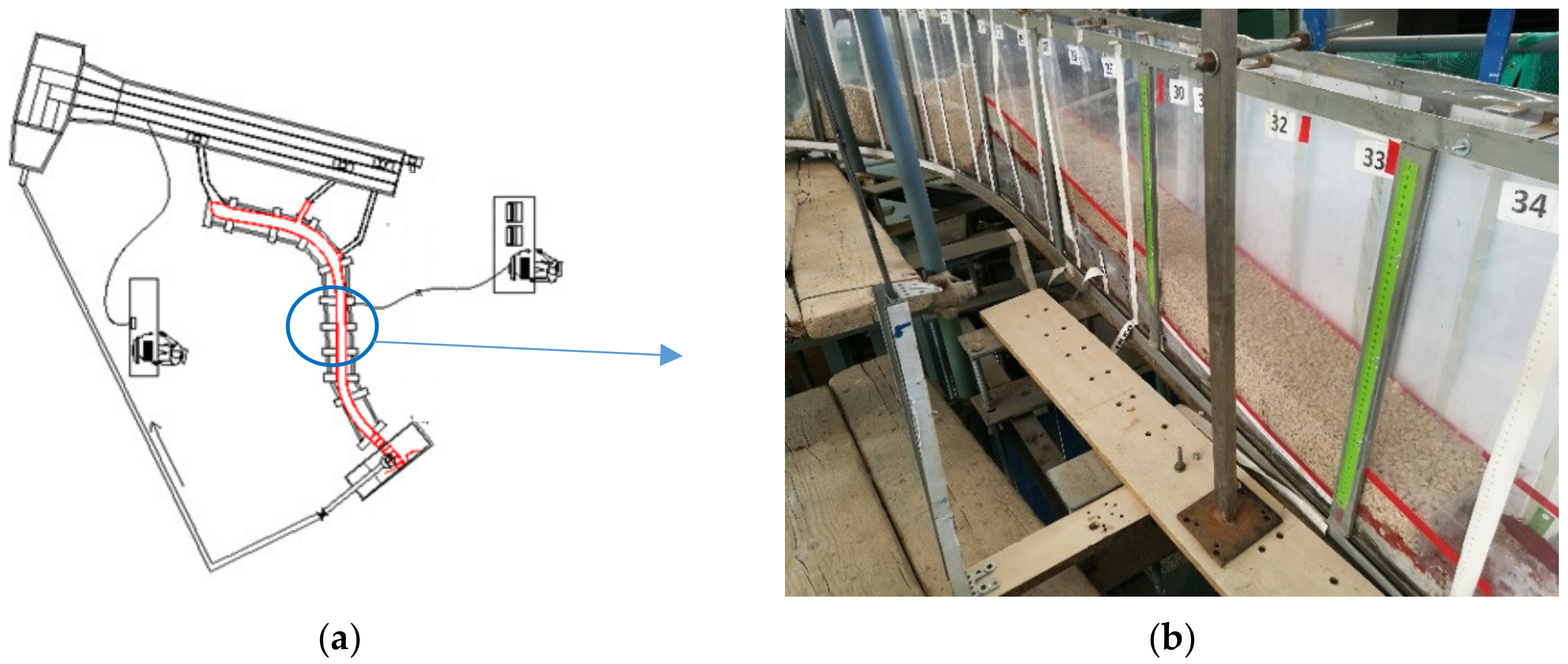
In order to analyze the velocity and grains concentration distributions within the debris body, data collected in a straight reach of a laboratory flume, constructed at the Department of Engineering, University of Palermo (Italy), have been used. The channel was 0.17 m wide and with Perspex transparent side-walls (see Figure 1). For the experimental run considered in the present work, the bed slope was 15° and consisted of assorted gravels with mean diameter D50 = 3 mm. These experimental conditions were selected after preliminary setting runs and in accordance with the indications of previous literature works [33,39,51,52].
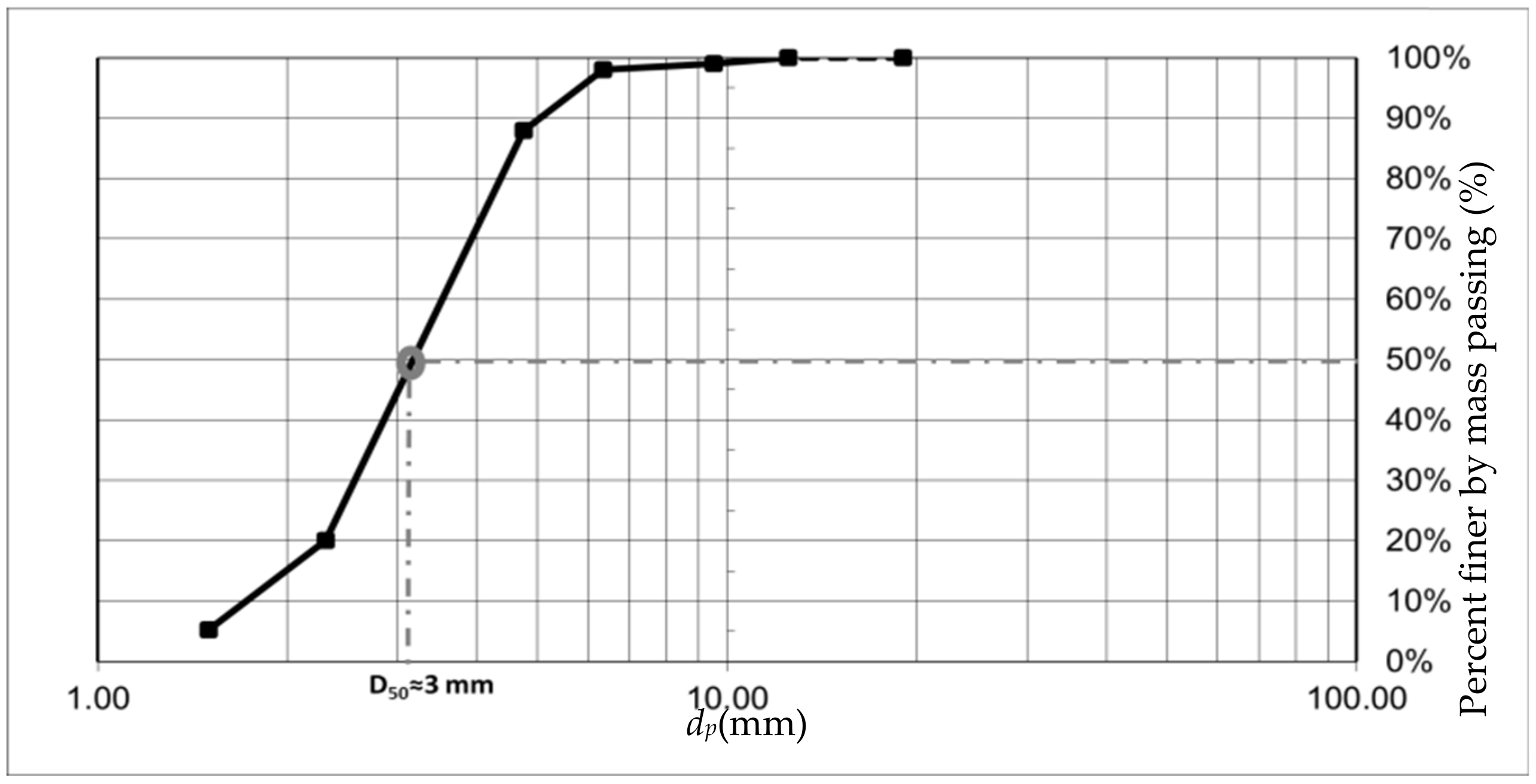
Figure 2 reports the grain-size distribution of the bed material, which was determined by using an electric oscillating sieve. The debris flow was generated by releasing the water discharge m3/s over a loose sediment layer of a thickness of around 0.10 m, which was previously saturated by slowly releasing a low water discharge Q0 = 0.8 × 10⁻³ m3/s. A permeable ground sill was positioned at the downstream end of the examined reach to avoid the degradation of the sediment layer.
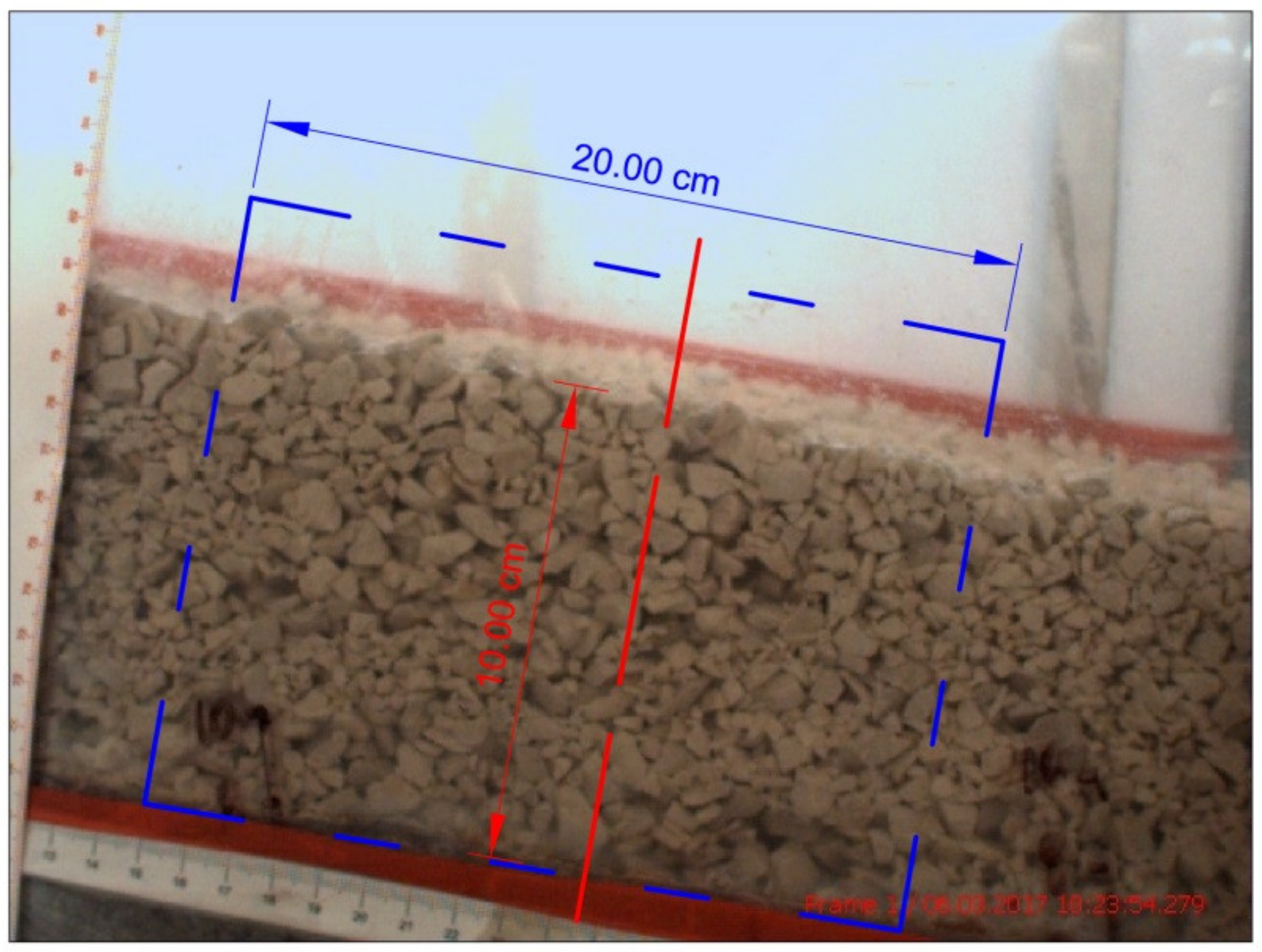
During the experiment, the water discharge was measured through the ultrasonic instrument Mainstream EH7000 (by Endress+Hauser S.p.a.), which is based on the Doppler effect, located in the upstream inflow channel. A high-resolution digital camera (AOS Technology AG) was used to record the flow motion through the transparent right side-wall. The camera was set at a frame rate of 300 fps, and the investigated area was around 20 cm wide (see Figure 3). The rate of the acquisition frequency was defined, during the preliminary runs, according to the camera’s characteristics and the extension of the covered area. During the passage of the debris body, around 600 frames were recorded. Furthermore, three samples of the mixture were taken at the free surface to estimate the free surface grains concentration Cs. Each sample was weighed, after having removed the water, with the help of a bake in order to determine the corresponding grain concentration. Finally, the “measured” free surface grain concentration was assumed as the mean value of the grain concentration of the three samples, which was equal to Cs,m = 0.305.
The frames recorded by the high-resolution camera during the passage of the debris body were used to estimate the instantaneous values both of the longitudinal velocity and the grain concentration at different distances, z, from the channel bed. To this aim, the sediment layer was divided into sub-layers, parallel to the channel bed, of thickness St = D50. Within each sub-layer of thickness St, the grain’s instantaneous longitudinal velocity, u(t), was estimated as the ratio between the grain’s displacement for two consecutive frames (i.e., two consecutive times) and the time interval. In particular, by considering the orthogonal local reference system with an origin at the southwest corner of the frame, it was estimated u(t) = (si+1 − si)/(ti+1 − ti) (where ti+1 and ti are two consecutive times and si+1 and si are the corresponding grain’s positions). Then, the time series of u(t), obtained for the grains within each sub-layer St by considering all the recorded frames, were used to determine both the corresponding time-averaged value u and the mean, , of the time-averaged velocities of the considered sub-layer St.
The recorded frames were also used to estimate the instantaneous values of the grain concentration within each sub-layer of thickness St. To this aim, a four-step procedure, appositely implemented in a Matlab environment and allowing us to count the grains in the considered sub-layer, was applied to each frame. Then, the time series of the grain concentration obtained for each sub-layer St were used to determine the corresponding time-averaged value C. Thus, the grain concentration distribution along the depth was analyzed by using the values of C obtained for all the sub-layers. The sensitivity analysis of the estimated grain concentration distribution with the value of the thickness St was also performed, as explained in the following Section 3.1.
3. Results
3.1. Grains Concentration Distribution
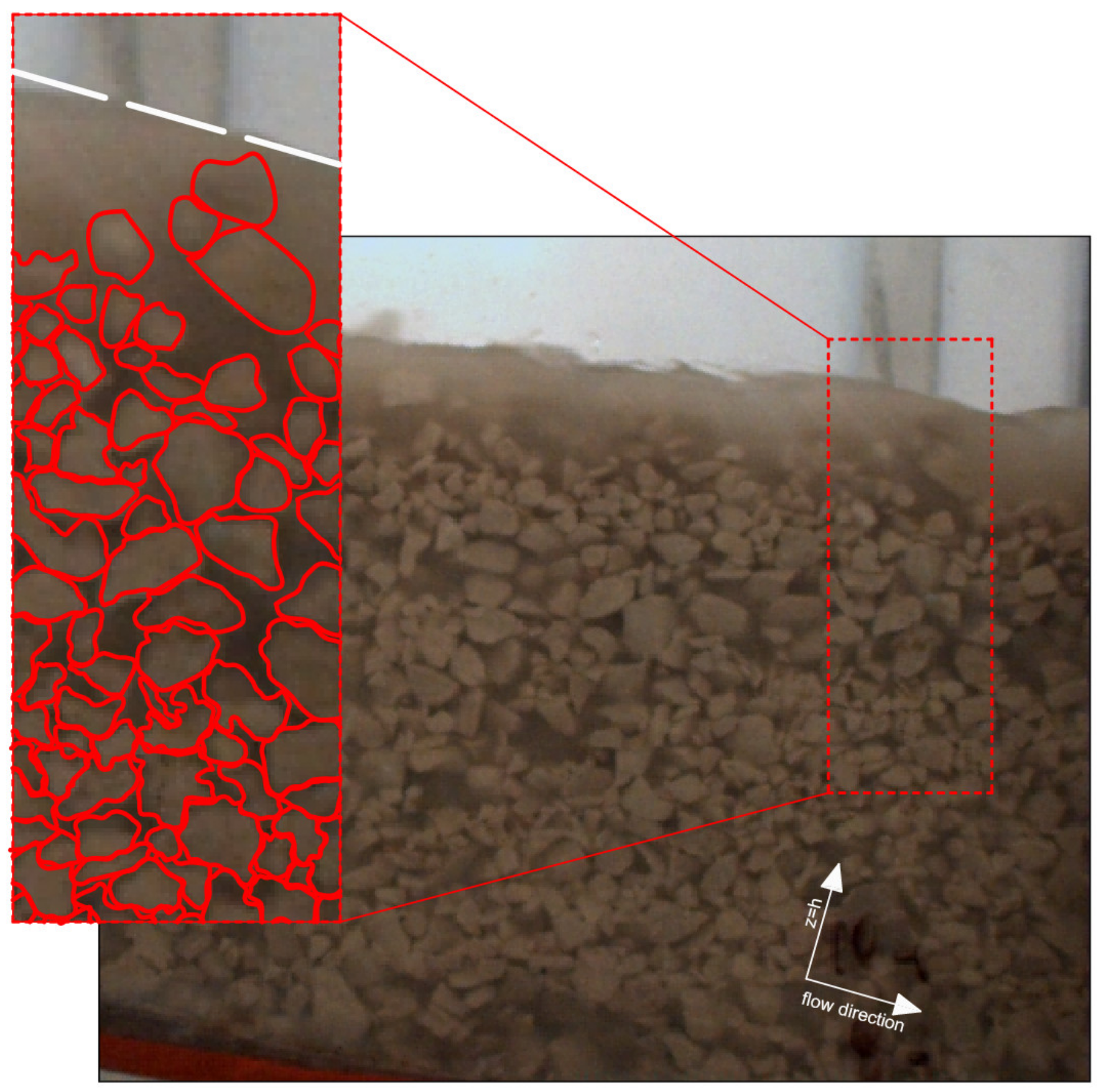
Both by the direct analysis during the experimental run and as a result of the aforementioned four-steps procedure, it was verified that the grain concentration varies along the direction orthogonal to the bed. In particular, as Figure 4 clearly shows, as one passes from the free surface to the bed, the movement of the grains decreases and the grain concentration increases. Close to the bed, the frictional stress is so high that no motion is possible (static configuration), and the grain concentration assumes its maximum value (i.e., the maximum packing concentration) C*. The thickness of the static bed, zo, was estimated from the analysis of both of the recorded frames and of the measured velocity profiles.
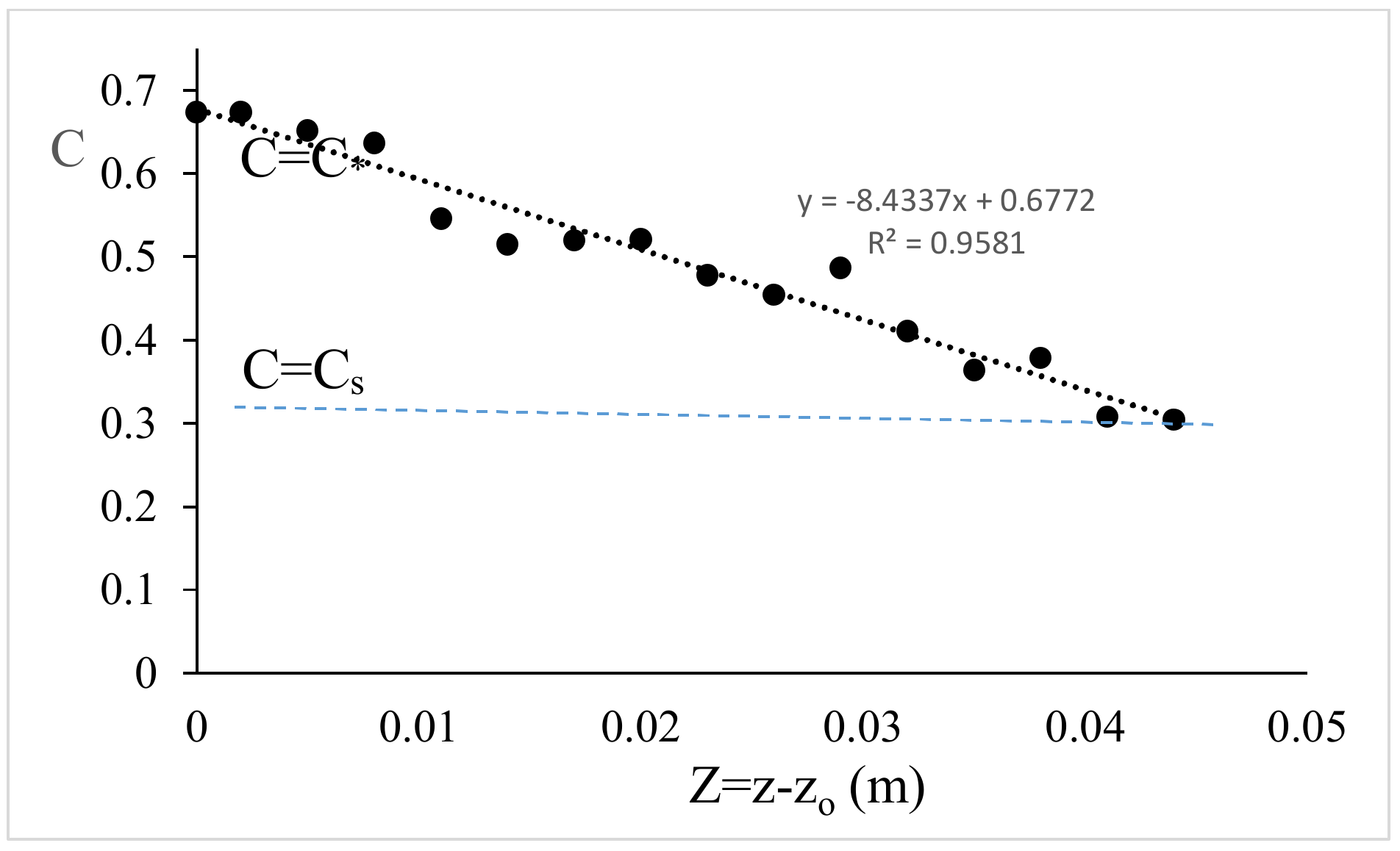
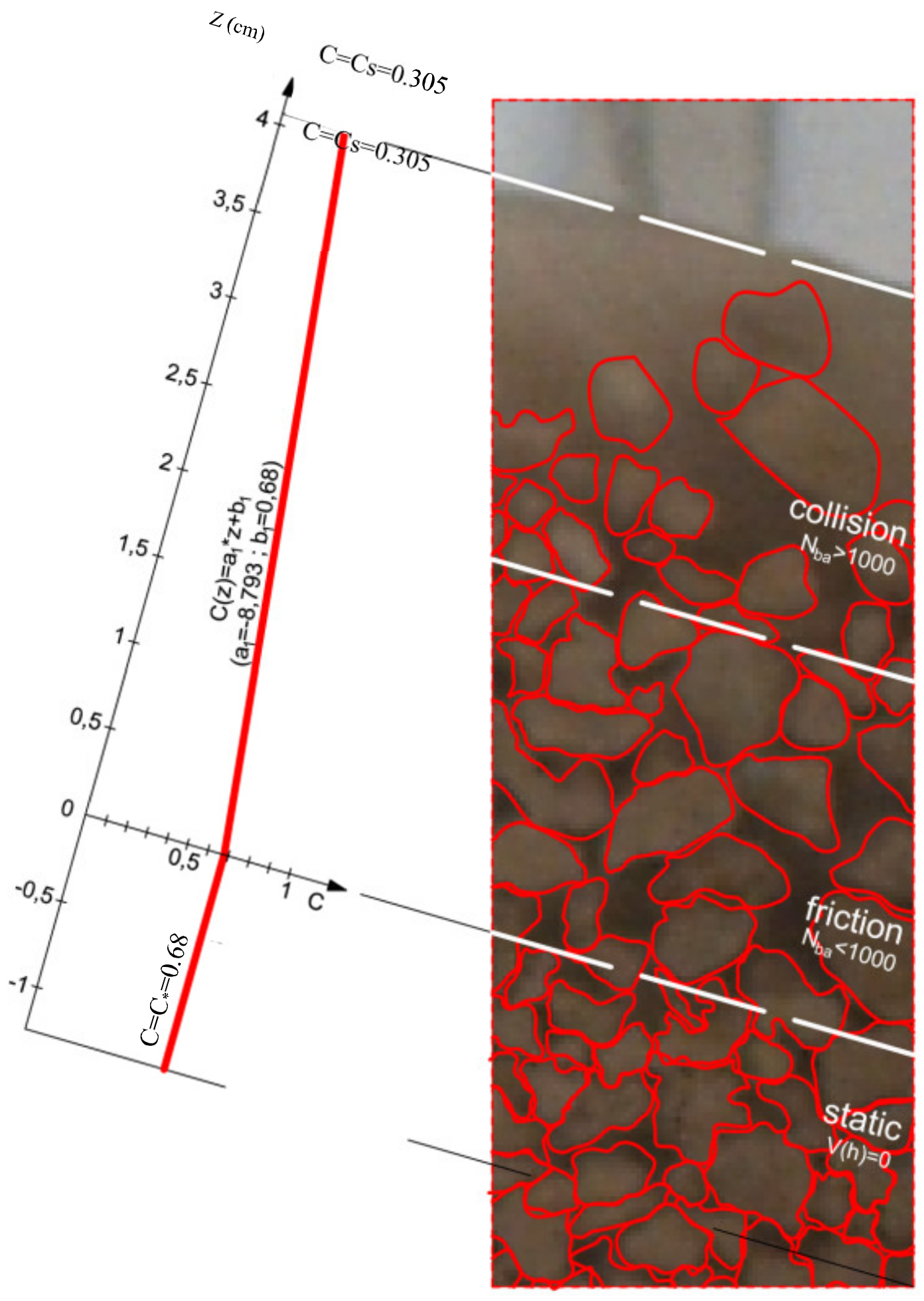
The values of grain concentration C obtained for all the sub-layers were plotted against the distance from the upper level of the static bed, as reported in Figure 5.
As Figure 5 shows, the points can be interpolated by a linear law (with regression coefficient R2 = 0.96). The values of the grain concentration at the extreme points of the interpolating line are very close, respectively, to those of the surface concentration, Cs, and of the maximum possible concentration C* at the bed. Based on this, the following linear law is considered to approximate the distribution of the grain concentration
where C(z) indicates the value of the grain concentration at level z. Based on Equation (5), the variation of the grain concentration within the debris body can be estimated as a function of the two parameters C∗ and Cs.
For the present application, it is C∗ = 0.676 and Cs = 0.305, and thus Equation (5) can be written as .
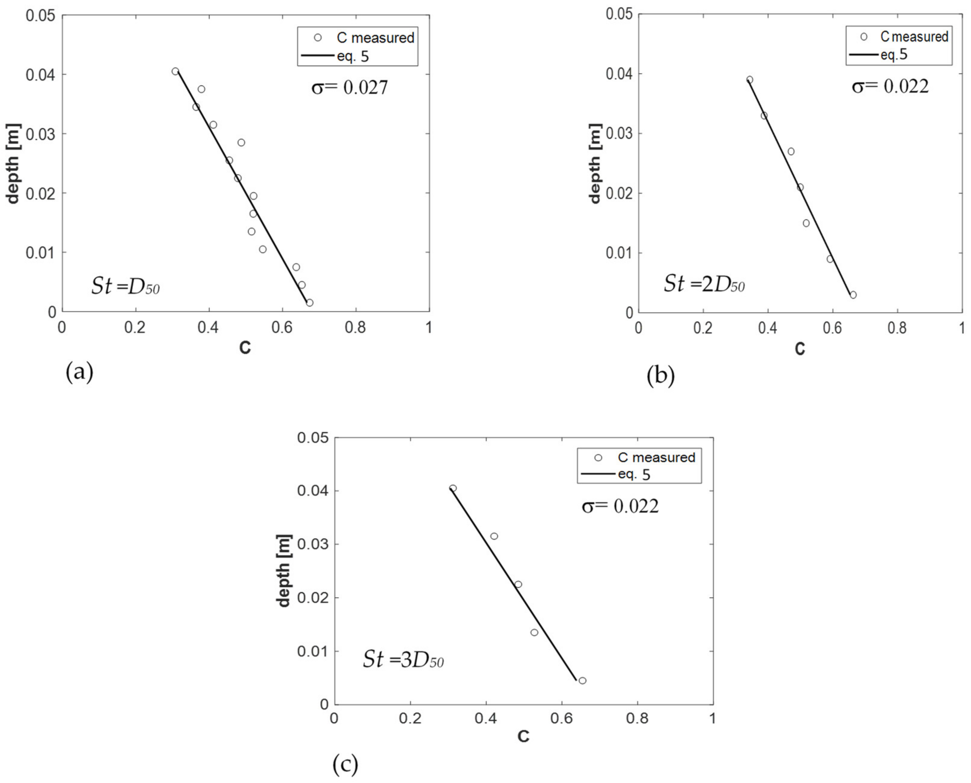
In order to investigate the sensitivity of the estimated grains concentration distribution to the thickness of the sub-layer, other two values of St have been considered (i.e., St = 2D50 = 6 mm; St = 3D50 = 9 mm) and the corresponding values of grain concentration C have also been estimated by applying the aforementioned four-step procedure. Then, the values of the grain concentration determined for each value of St were compared with the theoretical distribution given by Equation (5), as reported in Figure 6.
Figure 6 also reports the values of the root mean square error (σ) between the values of the grain concentration calculated in the i-th sub-layer by using Equation (5), Ci,c, and those measured, Ci,m:
where Nts is the number of the sub-layers of thickness St. It can be observed that σ assumes small and almost equal values for all the considered values of St. This suggests that the estimated grains concentration distribution does not depend on the selected value of St. Finally, a value of St = 2D50 (6 mm) has been assumed for the subsequent analysis.
3.2. Modified Bagnold’s Equation Applied to Debris Flow
Based on the results obtained in Section 3.1, Equation (3) is rewritten as follows:
with
where C(z) is given by Equation (5).
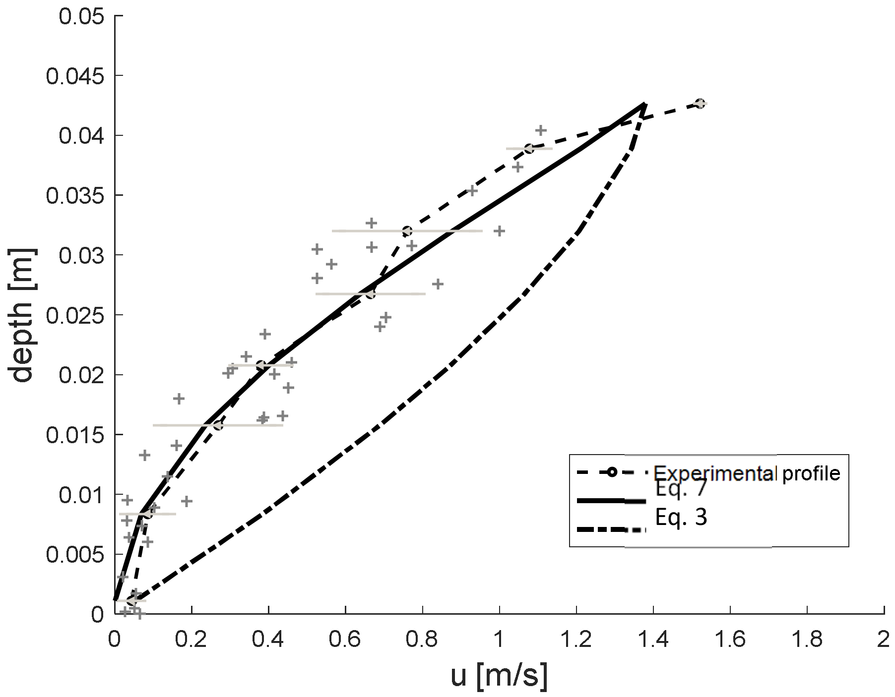
In Figure 7, the velocity profile estimated by applying Equation (7) is compared to that determined by applying Equation (3). This figure also reports both the profile of the mean measured velocity (indicated as “experimental profile”) and the velocity u of selected grains. From Figure 7, it is clear that while the velocity profile estimated by applying Equation (3) (i.e., with uniform grain concentration within the debris body) deviates from the experimental one, the velocity profile estimated by using Equation (7) (i.e., by considering the linear variation of the grain concentration within the debris body) well approximates the experimental profile.
This result indicates that Equation (5) well interprets the variation of the grain concentration within the debris body, also confirming that the assumption of uniform grain concentration in the entire flow depth is not realistic.
Thus, the Bagnold number NBa has been rewritten as follows:
NBa(z) = [ρsγdp2λ(z)1/2]/μf
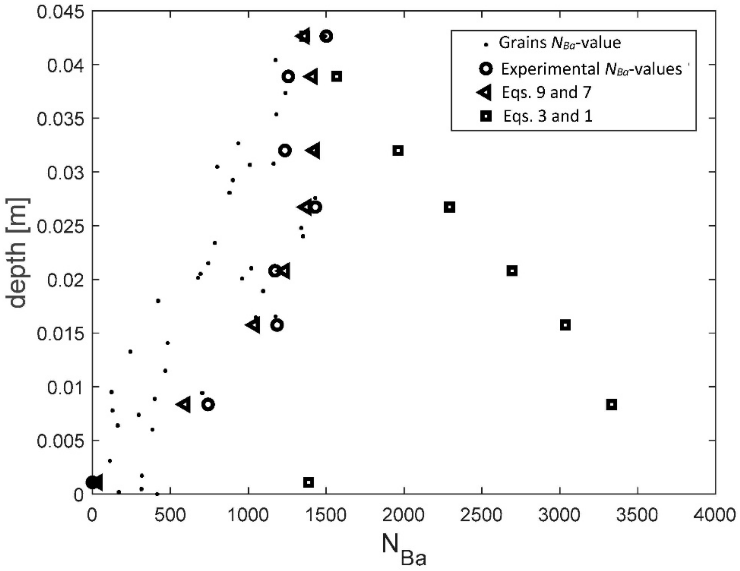
By applying Equation (9), the regime of flow motion has been identified in the entire depth of flow, as reported in Figure 8.
In particular, Figure 8 reports both the NBa-values obtained by using Equation (9), with the velocity and the grain concentration distributions respectively given by Equations (7) and (5), and the NBa-values (hereon indicated as “experimental NBa-values”) obtained by using the experimental velocity profile. Figure 8 also reports the NBa-values obtained by using Equations (1) and (3). Figure 8 shows that while the distribution of the NBa-values estimated by using Equation (9) is in agreement with the profile of the experimental NBa-values, the distribution of the NBa-values estimated by using Equation (1) deviates from it. In particular, the last one has NBa-values greater than 1000, close to the bed, and a decreasing trend as one passes from the bed to the free surface. On the contrary, Equation (9) determines NBa-values less than 1000 close to the bed and greater than 1000 close to the free surface. The latter trend of the NBa-values is consistent with that observed in previous literature works [34,48,51], indicating the development of the frictional flow regime for NBa-values <1000 and of the collisional-inertial flow regime for NBa-values >1000.
Based on the obtained results, it can be concluded that, in the present application, three different regimes of motion can be identified within the debris body (see Figure 9): the collisional regime close to the free surface with NBa-values >1000 and C ≅ Cs, the frictional regime in the intermediate zone with NBa-values <1000 and C = C(z), and the static zone close to the bed with NBa-values <<1000 and C ≅ C∗.
3.3. Free Surface Grains Concentration and Procedure for Its Estimation
Based on Equation (7), the longitudinal velocity profile should be determined as a function of the variation of the grain concentration defined by Equation (5) and, thus, as a function of the parameters C* and Cs. While the parameter C∗ could be easily identified, as mentioned in Section 2.1, it is difficult to determine the free surface grain concentration, Cs.
Thus, in this part of the work, experimental velocity profiles taken from the literature, i.e., data from [33,35,37,39] were considered and the parameter Cs was determined by minimizing the mean square error between the velocity values determined by using Equation (7) and the experimental ones:
where n is the number of the measurement points, um,i and uc,i indicate, respectively, the measured and the calculated velocity values in the i-th sub-layer.
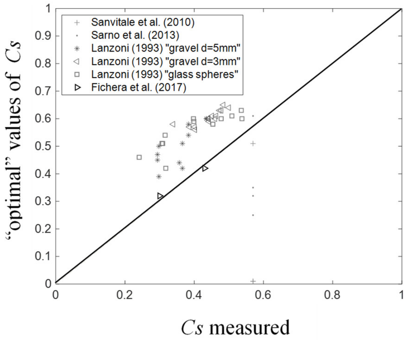
Figure 10 shows the comparison between the values of the parameter Cs obtained as a result of the minimization process (indicated as “optimal” values of Cs) and those taken from the literature [33,35,37,39]. The line of the perfect agreement is also reported in Figure 10. From this figure, it can be observed that, generally, the “optimal” values of Cs are slightly greater than those measured, and a very good agreement between the “optimal” values of Cs and those measured by Fichera et al. [39] can be observed. The different behavior observed in the latter case could be due to the fact that while Fichera et al. [39] measured the free surface concentration during the passage of the debris body in the examined reach, as well as in the present work, the other values of Cs were measured either not during the passage of the debris body or in sections different from those examined or not at the free surface. This further indicates the importance of the correct definition of the parameter Cs.
In order to identify a more generalizable procedure to estimate Cs, it has been taken into account that, according to Armanini et al. [34] (see also in [51]), in a flowing layer of grains over a loose bed of inclination β, fully saturated with water, and, with grain concentration assumed coincident with the transport concentration Cs, it is
where φc represents the critical friction angle.
For negligible interstitial overpressures (as it occurs at the free surface), in Equation (11), φc could be assumed equal to the static friction angle of the material. This means that Equation (11) would allow us to obtain information on the grain concentration Cs, starting from the knowledge of the bed slope and of the static friction angle, which can be determined by simple shear tests.
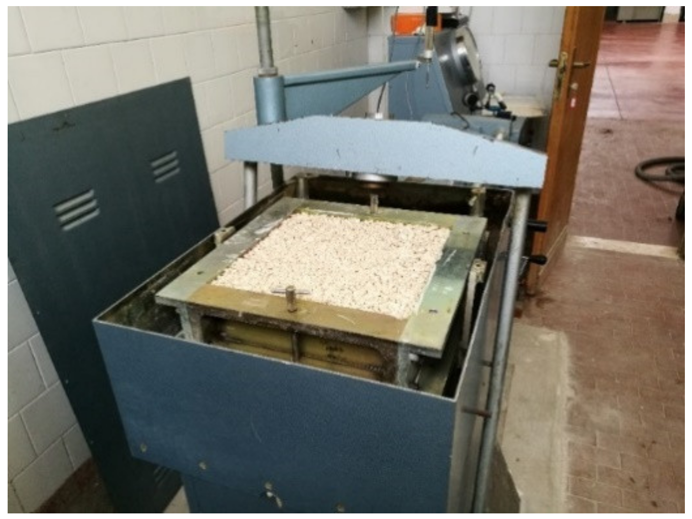
Thus, the existence of the relationship (Equation (11)) between the static friction angle and the concentration Cs is explored for the present application. To this aim, the static friction angle φc was determined by using the direct cutting apparatus available at the Geotechnical Laboratory of the Engineering Department, University of Palermo. Such an apparatus is specially adapted to the present application because it is equipped by a large cutting box (30 × 30 × 20 cm3—see Figure 11), allowing us to test a sample, of adequate volume, of the material used for the experimental run.
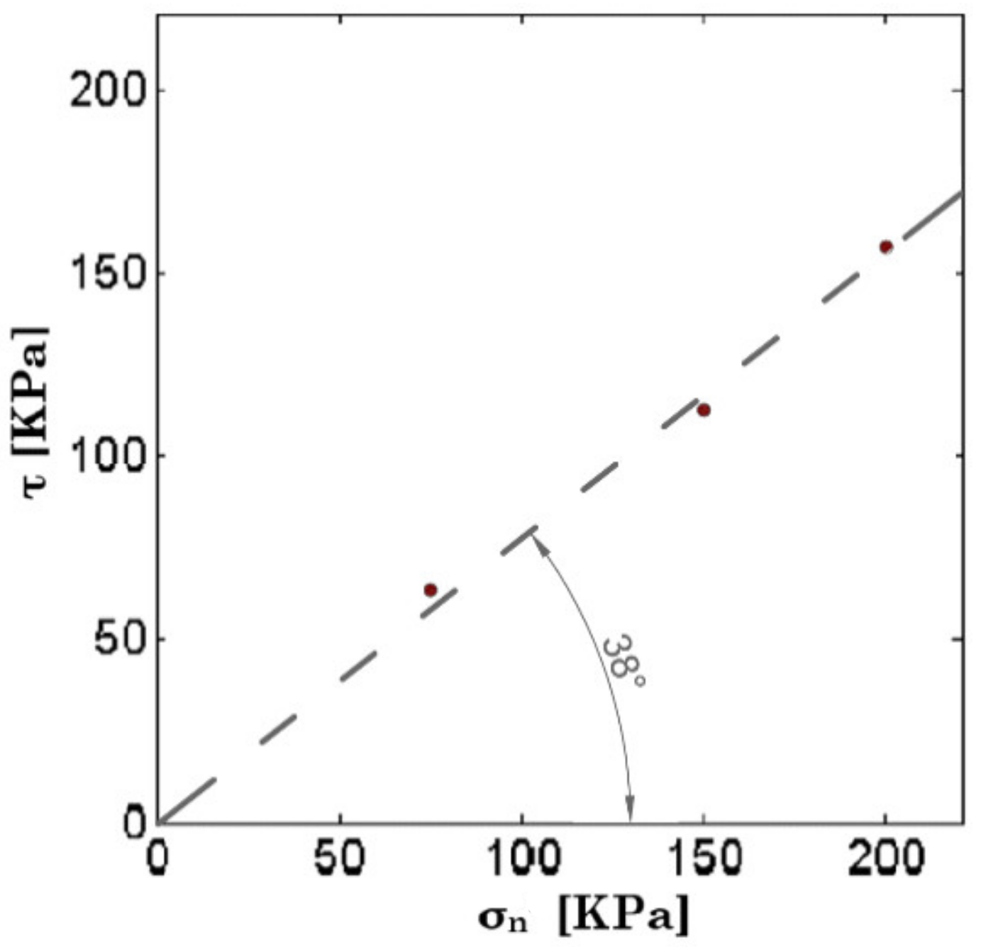
The cutting tests were performed, at a constant volume and in saturated conditions, for three samples of the debris body by inducing a constant horizontal force. As a result, the relation between the cutting shear stress, τ, and the corresponding cutting force, σn, was obtained for each test. More details of the testing procedure can be found in Fichera [53]. From the cutting tests, it was also verified that all the examined samples assumed a very similar behavior. By considering the maximum value of the shear stress, τmax, of each test, the couples of values [τmax, σn] were reported on a Cartesian plane. As Figure 12 shows, the coupled values [τmax, σn] are arranged around an interpolating line, having an angular coefficient equal to φc,e = 38°. Such an angular coefficient represents the “experimental” value of the static friction angle of the used granular material.
Then, the static friction angle was also determined from Equation (11) by considering that, for the examined case, the measured surface grain concentration is Cs,m = 0.305 and the inclination is β = 15°. Finally, a value φc = 38° was obtained from Equation (11). It is clear that this value of φc is equal to that obtained from the aforementioned direct cutting tests.
Thus, it can be concluded that, in the first approximation, the free surface grain concentration, Cs, can be estimated by applying Equation (11), starting from the knowledge of the bed slope and of the static friction angle of the material.
4. Discussion
4.1. Velocity Profiles and Comparisons with Literature Data
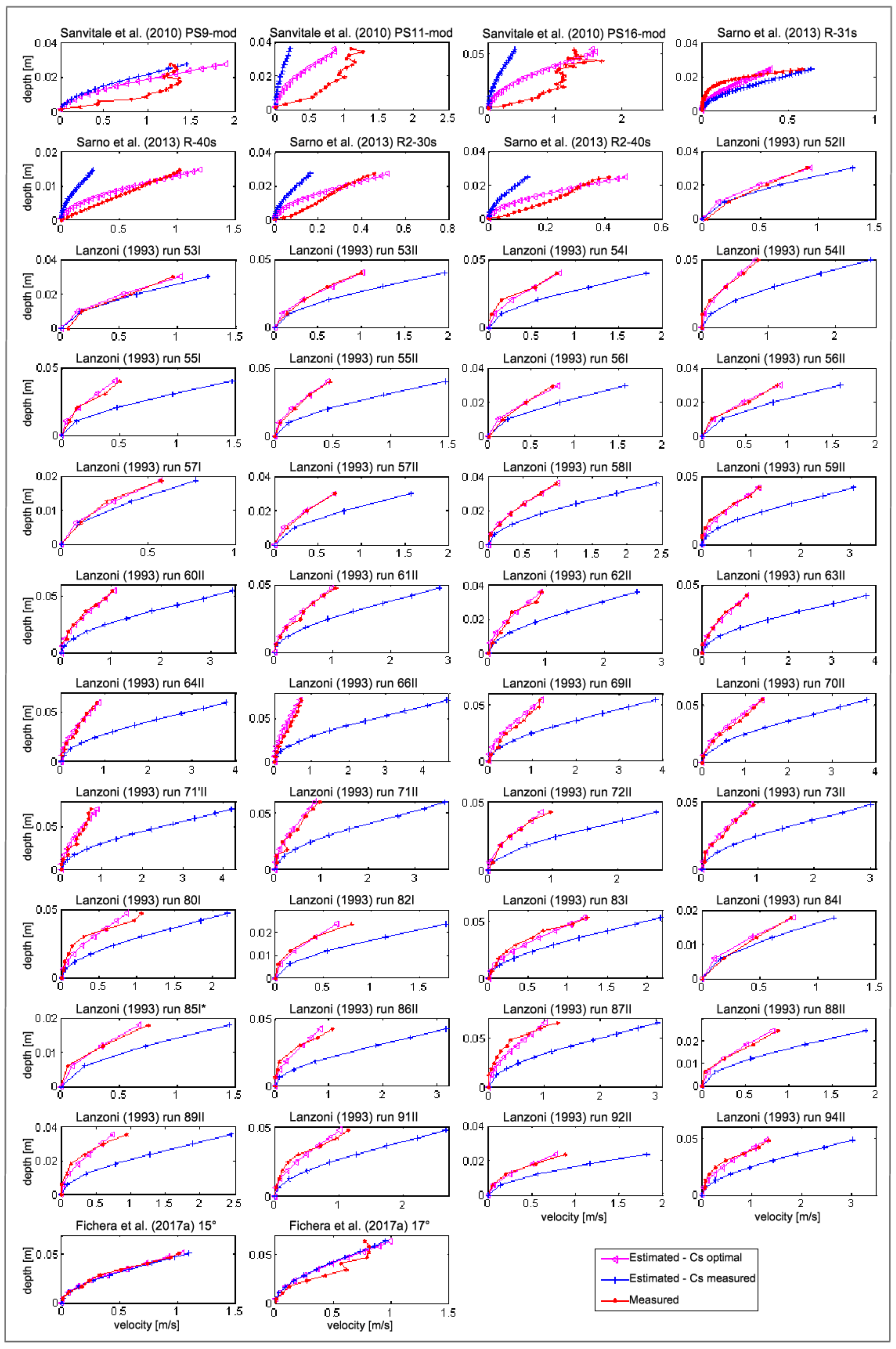
The applicability of the Equations (5) and (7) was also assessed by comparing the estimated velocity profiles with measured velocity profiles taken from the literature. In particular, measured profiles taken from Lanzoni [33] (see also in [53,54]), Sanvitale et al. [35], Sarno et al. [37], and Fichera et al. [39] were considered. In total, measured profiles from 46 pieces of literature were used for the comparison.
In Figure 13, the velocity profiles estimated by using Equations (5) and (7) are compared with those measured. In particular, this figure reports the velocity profiles estimated by assuming for the parameter Cs both the values taken from the literature and the calculated “optimal” values.
It can be seen that, while in the first case the estimated velocity profiles differ from those measured when the “optimal” values of Cs are used, the estimated velocity profiles compare well with the measured ones and, with the exception of the comparisons with SanVitale et al.’s [35] data, a value of the mean square error less than 0.1 is obtained. The differences obtained within the debris body between the estimated velocity profiles and those measured by SanVitale et al. [35] could be related to the fact that SanVitale et al. [35] analyzed a fluid/sediment mixture (consisting of borosilicate glass and hydrocarbon oil) of chemical/physical characteristics different from those examined by the other authors. This confirms previous literature findings indicating that the chemical/physical characteristics of the material could affect the stress distribution and, thus, the behavior of the fluid/sediment mixture (see, as examples, [55,56]).
Thus, on the one hand, Figure 13 demonstrates that Equation (7) allows us to correctly interpret the velocity distribution within the debris body by taking into account the grain concentration variation through Equation (5); on the other hand, it confirms the importance of the correct definition of the parameter Cs. Based on the results presented in Section 3.3, Cs could be determined either by direct measurements during the passage of the debris body or by applying Equation (11) as a function of the static friction angle of the material.
4.2. Main Aspects Derived by the Proposed Modified Expressions and Procedure
As mentioned in the introduction, in natural environments, stony-type debris flows can be generated in rapid valleys and in high slope streams [1,2]. In these types of debris flows, in which finer sediments do not affect the overall behavior of the mixture, the assumption of the grain concentration being uniform everywhere is generally accepted in analyzing flow dynamics [11,12,14].
The analysis conducted in the present work has substantially highlighted that the identification of the grain concentration distribution within the debris body as an important aspect in estimating the velocity profile. In particular, the presented experiment has provided useful information on the distribution of the grain concentration within the debris body. It has been observed that as one passes from the free surface towards the bed, the grain concentration increases, and the movement of the grains decreases. At the bed, the frictional stress is so high that no motion is possible, the static configuration is obtained, and the grain concentration assumes its maximum value (i.e., the so-called maximum packing concentration), C*. This confirms that the assumption of uniform sediment distribution in the entire depth, which is generally used in analyzing the hydrodynamics of stony-debris flow, is not realistic.
The analysis of the measured values of the grain concentration has shown that the grain concentration distribution within the debris body can be approximated by a linear law, which can be identified starting from the knowledge of the maximum packing concentration at the bed, C*, and the value of the grain concentration at the free surface, Cs.
Furthermore, the obtained results have shown that the variation of grain concentration along the depth strongly affects the grains’ mobility, thus confirming previous literature findings [13,51] suggesting the development of a spatially variable behavior and stress regime within the debris flow.
By considering the obtained linear law of the grain concentration distribution, modified expressions of Bagnold’s number NBa and of the velocity for stony-type debris flows have been obtained.
The analysis of the values of Bagnold’s number (NBa), estimated by using the aforementioned modified expression, has highlighted that three different flow regimes can be identified within the debris body. In particular, the collisional regime is obtained close to the free surface, where the grain concentration is C = Cs and the NBa-values are greater than 1000; the frictional regime is obtained in the intermediate zone, where C = C(z) and the NBa-values are lower than 1000; close to the bed, where the concentration is C = C* and the NBa-values are strongly lower than 1000, the static zone is established. The observed behavior is consistent with results obtained in other literature works (see in [34,51,53]), indicating the development of the frictional flow regime for NBa-values <1000 and of the collisional-inertial flow regime for NBa-values >1000.
The proposed modified expression to estimate the velocity in stony-type debris flows allows us to evaluate the flow velocity profile within the debris body as a function of two parameters, that are the maximum packing concentration, C*, and free surface concentration, Cs. While parameter C* can be easily identified by using physically-based literature data, it is difficult to determine parameter Cs. Thus, first, the “optimal” values of parameter Cs were calculated by minimizing the mean square error between the velocity values estimated by using the proposed expression and the experimental ones taken from the literature. As is clear from the previous subsection, this analysis has allowed us to highlight the important role of parameter Cs in defining the velocity distribution within the debris body. The comparison between the velocity profiles estimated by considering the “optimal” values of Cs and the literature’s measured profiles (from [33,35,37,39]) has demonstrated that the proposed modified expression, which takes into account the variation of the grain concentration within the debris body, correctly interprets the measured velocities.
A useful general procedure for estimating free surface concentration Cs is also provided by using the results of cutting tests, also performed in the ambit of the present study, of a sample of the granular material used for the experimental run. Based on the relationship between the grain concentration and the bed slope, according to Armanini et al. [34], it has been verified that, in first approximation, surface grain concentration Cs could be determined, starting from the knowledge of the bed slope and of the static friction angle of the material, which could be easily estimated by simple direct cutting tests.
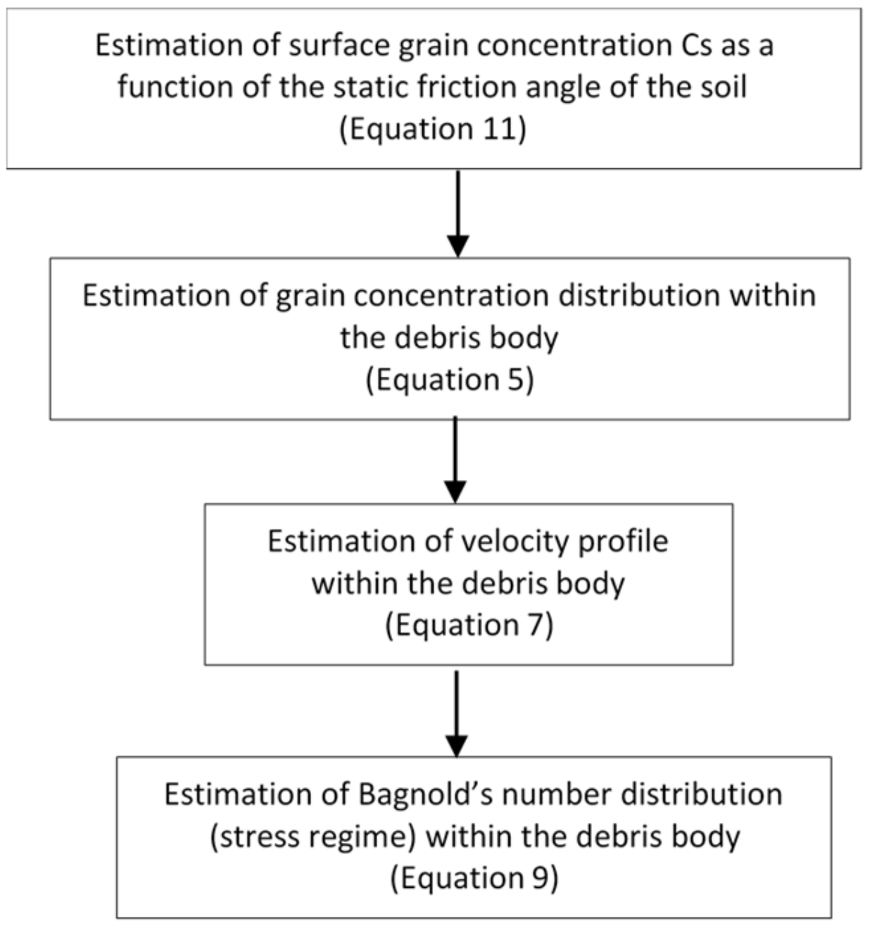
In summary, based on the aforementioned considerations, the use of the proposed expressions allows us to easily estimate the velocity profile and the stress regime variation within the debris body according to the procedure shown in the flow chart of Figure 14.
5. Conclusions
The present work deals with the dynamics of stony-type debris flows, focusing attention on the velocity and grain concentration distributions. The results obtained can be summarized as follows:
- (1)
- the distribution of the grain concentration can be interpreted by a linear law obtained between the value of the maximum package value, C*, at the bed and the value of the free surface concentration, Cs;
- (2)
- by removing the hypothesis of uniform grain concentration along the entire depth, modified expressions of Bagnold’s number and of the longitudinal velocity, which take into account the variation of the grain concentration in the entire depth, are presented. The expression of the velocity profile includes two parameters: the maximum package value, C*, which could be determined by using either experimental data appositely collected or physically-based literature data, and the value of the free surface concentration, Cs;
- (3)
- by using the modified expression of Bagnold’s number, it has been verified that a varying stress regime can develop within the debris flow. The NBa-values are strongly lower than 1000 when close to the bed (frictional regime) and are greater than 1000 (collisional-inertial regime) when close to the free surface;
- (4)
- it has been verified that, in the first approximation, surface concentration Cs can be estimated as a function of the static friction angle of the material, which can be determined by simple shear tests.
In summary, based on the results presented in this work, the velocity and the grain concentration distributions within the debris body can be estimated, starting from the knowledge of parameters C* and Cs that can be easily identified through physically-based literature data and by simple shear tests, respectively. This result is of great importance, especially in numerical modeling of stony-type debris flows, which in nature especially occur in rapid valleys or in high-slope streams.
Author Contributions
Conceptualization, D.T. and A.F.; methodology, D.T. and A.F.; validation, D.T. and A.F.; formal analysis, D.T.; investigation, A.F.; resources, D.T. and A.F.; data curation, A.F.; writing—original draft preparation, D.T.; writing—review and editing, D.T.; visualization, A.F.; supervision, D.T. and A.F. All authors have read and agreed to the published version of the manuscript.
Funding
This research received no external funding.
Acknowledgments
This work was partially supported by Italian National Research Programme PRIN 2017, with the project “IntEractions between hydrodyNamics flows and bioTic communities in fluvial Ecosystems: advancement in dischaRge monitoring and understanding of Processes Relevant for ecosystem sustaInability by the development of novel technologieS with fIeld observatioNs and laboratory testinG (ENTERPRISING)”.
Conflicts of Interest
The authors declare no conflict of interest.
References
- Takahashi, T. Debris flow. Annu. Rev. Fluid Mech. 1981, 13, 57–77. [Google Scholar] [CrossRef]
- Cannon, S.; Gartner, J.; Wilson, R.C.; Bowers, J.C.; Laber, J. Storm rainfall conditions for floods and debris flows from recently burned areas in south western Colorado and southern California. Geomorphology 2008, 96, 250–269. [Google Scholar] [CrossRef]
- Theule, J.I.; Liébault, F.; Laigle, D.; Loye, A.; Jaboyedoff, M. Channel scour and fill by debris flows and bedload transport. Geomorphology 2015, 243, 92–105. [Google Scholar] [CrossRef]
- Iverson, R.M. The physics of debris flows. Rev. Geophys. 1997, 35, 245–296. [Google Scholar] [CrossRef] [Green Version]
- Kaitna, R.; Rickenmann, D.; Schatzmann, M. Experimental study on rheologic behaviour of debris-flow material. Acta Geotech. 2007, 2, 71–85. [Google Scholar] [CrossRef]
- Armanini, A. Granular flows driven by gravity. J. Hydraul. Res. 2013, 51, 111–120. [Google Scholar] [CrossRef]
- Van Rijn, L.C. Sediment transport, part I: Bed load transport. J. Hydraul. Eng. 1984, 110, 1431–1456. [Google Scholar] [CrossRef] [Green Version]
- Van Rijn, L.C. Sediment transport, part II: Suspended load transport. J. Hydraul. Eng. 1984, 110, 1613–1641. [Google Scholar] [CrossRef]
- Joshi, S.; Xu, Y.J. Assessment of suspended sand availability under different flow conditions of the Lowermost Mississippi River at Tarbert Landing during 1973–2013. Water 2015, 7, 7022–7044. [Google Scholar] [CrossRef]
- Joshi, S.; Xu, Y.J. Bedload and suspended load transport in the 140-km reach downstream of the Mississippi River avulsion to the Atchafalaya River. Water 2017, 9, 716. [Google Scholar] [CrossRef] [Green Version]
- Campbell, C.S. Granular shear flows at the elastic limit. J. Fluid Mech. 2002, 465, 261–291. [Google Scholar] [CrossRef]
- Campbell, C.S. Stress-controlled elastic granular shear flows. J. Fluid Mech. 2005, 539, 273–297. [Google Scholar] [CrossRef] [Green Version]
- Kaitna, R.; Dietrich, W.E.; Hsu, L. Surface slopes, velocity profiles and fluid pressure in coarse-grained debris flows saturated with water and mud. J. Fluid Mech. 2014, 7, 377–403. [Google Scholar] [CrossRef]
- Takahashi, T. Debris Flows: Mechanics, prediction and countermeasures. Balkema-Proc and Monogr. In Eng., Water and Earth Sc.; Taylor and Francis: New York, NY, USA, 2007. [Google Scholar]
- Bonnet-Staub, I. Definition d’une typologie des deposits de laves torrentielles et identification de critres granulomtriques et geotechniques concernant les zones sources. J. Bull. Eng. Geol. Environ. 1999, 57, 359–367. [Google Scholar] [CrossRef]
- Bagnold, R.A. Experiments on a gravity-free dispersion of large solid spheres in a Newtonian fluid under shear. Proc. R. Soc. Lond. A 1954, 225, 49–63. [Google Scholar]
- Hunt, M.; Zenit, R.; Campbell, C.S.; Brennen, C.E. Revisiting the 1954 suspension experiments of RA Bagnold. J. Fluid Mech. 2002, 452, 1–24. [Google Scholar] [CrossRef] [Green Version]
- Bagnold, R.A. The shearing and dilation of dry sand and the ‘singing’ mechanism. Proc. R. Soc. Lond. A 1966, 295, 219–232. [Google Scholar]
- Bagnold, R.A. An empirical correlation of bedload transport rates in flumes and natural rivers. Proc. R. Soc. Lond. A 1980, 372, 453–473. [Google Scholar]
- Egashira, S.; Miyamoto, K.; Itoh, T. Constitutive equations of debris flow and their applicability. In Proceedings of the 1st International Conference on Debris-Flow Hazards Mitigation: Mechanics, Prediction, and Assessment, San Francisco, CA, USA, 7–9 August 1997; pp. 340–349. [Google Scholar]
- Iverson, R.M.; Denlinger, R.P. Flow of variably fluidized granular masses across three-dimensional terrain: Coulomb mixture theory. J. Geophys. Res. 2001, 106, 537–552. [Google Scholar] [CrossRef]
- Iverson, R.M. Elementary theory of bed-sediment entrainment by debris flows and avalanches. J. Geophys. Res. 2012, 117, F03006. [Google Scholar] [CrossRef]
- Iverson, R.M.; Ouyang, C. Entrainment of bed material by Earth-surface mass flows: Review and reformulation of depth-integratedtheory. Rev. Geophys. 2015, 53, 27–58. [Google Scholar] [CrossRef]
- Hungr, O.; McDougall, S.; Bovis, M. Entrainment of material by Debris flows. In Debris-Flow Hazards and Related Phenomena; Jakob, M., Hungr, O., Eds.; Springer: Berlin/Heidelberg, Germany, 2005; pp. 135–158. [Google Scholar]
- Scheidl, C.; Rickenmann, D. Empirical prediction of debris-flow mobility and deposition on fans. Earth Surf. Process. Landf. 2009, 35, 157–173. [Google Scholar] [CrossRef]
- Berger, C.; McArdell, B.W.; Schlunegger, F. Direct measurement of channel erosion by debris flows, Illgraben, Switzerland. J. Geophys. Res. 2011, 116, F01002. [Google Scholar] [CrossRef] [Green Version]
- Chiodi, F.; Claudin, P.; Andreotti, B. A two-phase flow model of sediment transport: Transition from bedload to suspended load. J. Fluid Mech. 2014, 755, 561–581. [Google Scholar] [CrossRef] [Green Version]
- Thibaud, R.; Chauchat, J. A two-phase model for sheet flow regime based on dense granular flow rheology. J. Geophys. Res. Am. Geophys. Union 2013, 118, 619–634. [Google Scholar]
- Chapman, S.; Cowling, T.G. The Mathematical Theory of Non-Uniform Gases, 3rd ed.; Cambridge University Press: Cambridge, UK, 1971. [Google Scholar]
- Jenkins, J.T.; Savage, S.B. A theory for rapid flow of identical, smooth, nearly elastic, spherical particles. J. Fluid Mech. 1983, 130, 186–202. [Google Scholar] [CrossRef]
- Lun, C.K.K.; Savage, S.B.; Jeffrey, D.J.; Chepurniy, N. Kinetic theories for granular flow: Inelastic particles in Couette flow and slightly in elastic particles in a general flow field. J. Fluid Mech. 1984, 140, 223–256. [Google Scholar] [CrossRef]
- Jenkins, J.T.; Richman, M.W. Kinetic theory for plane flows of a dense gas of identical, rough, inelastic, circular disks. Phys. Fluids 1985, 28, 3485–3494. [Google Scholar] [CrossRef]
- Lanzoni, S. Meccanica di miscugli solio-liquido in regime granulo-inerziale. Ph.D. Thesis, University of Padova, Padua, Italy, 1993. [Google Scholar]
- Armanini, A.; Capart, H.; Fraccarollo, L.; Larcher, M. Rheological stratification in experimental free-surface flows of granular-liquid mixtures. J. Fluid Mech. 2005, 532, 269–319. [Google Scholar] [CrossRef] [Green Version]
- Sanvitale, N.; Bowman, E.T.; Genevois, R. Experimental measurements of velocity through granular-liquid flows. Ital. J. Eng. Geol. Environ. Book Casa Editrice Università La Sapienza 2010. [Google Scholar] [CrossRef]
- Iverson, R.M.; Logan, M.; Lahusen, R.G.; Berti, M. The perfect debris flow? Aggregated results from 28 large-scale experiments. J. Geophys. Res. 2010, 115, F03005. [Google Scholar]
- Sarno, L.; Papa, M.N.; Tai, Y.C.; Carravetta, A.; Martino, R. A reliable PIV approach for measuring velocity profiles of highly sheared granular flows. In Latest Trends in Engineering Mechanics, Structures, Engineering Geology. 2013. ISBN: 978-960-474-376-6. Available online: https://www.researchgate.net/publication/278961892_A_reliable_PIV_approach_for_measuring_velocity_profiles_of_highly_sheared_granular_flows (accessed on 13 May 2020).
- Hsu, L.; Dietrich, W.E.; Sklar, L.S. Experimental study of bedrock erosion by granular flows. J. Geophys. Res. 2008, 113, F02001. [Google Scholar] [CrossRef]
- Fichera, A.; Stancanelli, L.M.; Lanzoni, S.; Foti, E. Stony Debris Flow Debouching in a River Reach: Energy Dissipative Mechanisms and Deposit Morphology. In Proceedings of the Workshop on World Landslide Forum, Ljubljana, Slovenia, 9 May–2 June 2017; Springer: Cham, Switzerland, 2017; pp. 377–383. [Google Scholar]
- Marchi, L.; Dalla Fontana, G. GIS morphometric indicators for the analysis of sediment dynamics in mountain basins. Environ. Geol. 2005, 48, 218–228. [Google Scholar] [CrossRef]
- Gruber, S.; Huggel, C.; Pike, R. Modelling mass movements and landslide susceptibility. In Geomorphometry; Hengl, T., Reuter, H.I., Eds.; Elsevier: Amsterdam, The Netherlands, 2008; pp. 527–550. Available online: http://www.zora.uzh.ch/id/eprint/6475/ (accessed on 13 May 2020).
- Takahashi, T. Mechanical characteristics of debris flow. J. Hydraulics Div. ASCE 1978, 104, 1153–1169. [Google Scholar]
- Takahashi, T. Debris flow on prismatic open channel. J. Hydraulics Div. ASCE 1980, 106, 1153–1169. [Google Scholar]
- Gregoretti, C.; Dalla Fontana, G. The triggering of debris flows due to channel-bed failure in some alpine headwater basins of Dolomites: Analyses of critical runoff. Hydrological Process. 2008, 22, 2248–2263. [Google Scholar] [CrossRef]
- Berti, M.; Genevois, R.; Simoni, A.; Tecca, P.R. Field observations of a debris flow event in the Dolomites. Geomorphology 1999, 29, 256–274. [Google Scholar] [CrossRef]
- Moscariello, A.; Marchi, L.; Maraga, F.; Mortara, G. Alluvial fans in the Italian Alps: Sedimentary facies and processes. In Flood & Megaflood Processes and Deposits—Recent and Ancient Example; Martini, P., Baker, V.R., Garzon, G., Eds.; Blackwell Science: Oxford, UK, 2002; pp. 141–166. [Google Scholar]
- Savage, S.B.; Lun, C.K.K. Particle size segregation in inclined chute flow of dry cohesionless granular solids. J. Fluid Mech. 1988, 189, 311–335. [Google Scholar] [CrossRef]
- Aharonov, E.; Sparks, D. Rigidity phase transition in granular packings. Phys. Rev. E 1999, 60, 6890–6896. [Google Scholar] [CrossRef]
- Takahashi, T. An occurrence mechanism of mud-debris flows, and their characteristics in motion. Annu. DPRI 1977, 20, 405–435. [Google Scholar]
- Tsai, Y.F.; Tsai, H.K.; Ch, Y.L. Study on the configurations of debris-flow fans. IJEGE 2011, 2011, 03.B-032. [Google Scholar]
- Lanzoni, S.; Gregoretti, C.; Stancanelli, L.M. Coarse-grained debris flow dynamics on erodible beds. J. Geophys. Res. Earth Surf. 2017, 122, 596–614. [Google Scholar] [CrossRef]
- Chen, S.C.; An, S. Flume experiment of debris flow confluence formed alluvial fan in the main channel. In River, Coastal and Estuarine Morphodynamics: RCEM 2007; Dohmen-Janssen, C.M., Hulscher, S.J.M.H., Eds.; Taylor and Francis: London, UK, 2007; pp. 829–835. [Google Scholar]
- Fichera, A. Analisi e caratterizzazione del comportamento di una colata detritica. Ph.D. Thesis, University of Enna “KORE”, Italy, Kore, 2017. [Google Scholar]
- Lanzoni, S.; Tubino, M. Rheometric experiments on mature debris flows. In Proceedings of the XXV International Association for Hydro-Environment, Tokyo, Japan, 30 August–3 September 1993. Editor: Japan Society of Civil Engineers, Local Organizing Committee of the XXV Congress, IAHR, 1993. [Google Scholar]
- ASM International Handbook Committee. Engineered Materials Handbook; Desk Edition 1995; ASM International: Novelty, OH, USA, 1995; ISBN 0-87170-283-5. [Google Scholar]
- Zhao, Y.; Liu, Z. Study of Material Composition Effects on the Mechanical Properties of Soil-Rock Mixtures. Hindawi. Adv. Civil Eng. 2018, 2018, 3854727. [Google Scholar] [CrossRef]
Figure 1.
(a) Plan view of the experimental apparatus; (b) particular of the channel reach considered for the analysis (bed slope = 15°; assorted gravels with mean diameter D50 = 3 mm; the numbers indicate the sections in which the channel was discretized).
Figure 1.
(a) Plan view of the experimental apparatus; (b) particular of the channel reach considered for the analysis (bed slope = 15°; assorted gravels with mean diameter D50 = 3 mm; the numbers indicate the sections in which the channel was discretized).

Figure 2.
Grain size distribution of the bed material (the x-axis indicates the grain diameter; the y-axis indicates the percent of finer by mass passing).
Figure 2.
Grain size distribution of the bed material (the x-axis indicates the grain diameter; the y-axis indicates the percent of finer by mass passing).

Figure 3.
Scheme of the investigated area (in blue).

Figure 4.
Variation of grains concentration in the depth of flow and particular of the grain configuration.
Figure 4.
Variation of grains concentration in the depth of flow and particular of the grain configuration.

Figure 5.
Measured grain concentrations C and interpolating law (Z indicates the direction orthogonal to the bed with an origin at the upper level of the static bed).
Figure 5.
Measured grain concentrations C and interpolating law (Z indicates the direction orthogonal to the bed with an origin at the upper level of the static bed).

Figure 6.
Comparison between the theoretical distribution of the grain concentration (Equation (5)) and the estimated values (C measured) by assuming different sub-layer thickness St: (a) for St = D50; (b) for St = 2D50; (c) for St = 3D50. The x-axis indicates the grain concentration; the y-axis indicates the distance from the upper level of the static bed.

Figure 7.
Comparison between the profile (experimental profile) and the estimated ones by applying Equation (3) and by applying Equation (7). The dots represent the velocity u of selected grains (the x-axis indicates the longitudinal velocity; the y-axis indicates the distance from the upper level of the static bed).

Figure 8.
Comparison between the NBa-values by using the experimental velocity profile (experimental NBa-values), the NBa-values estimated by applying Equations (9) and (7) and the NBa-values estimated by applying Equations (3) and (1). The dots represent the NBa-values of selected grains; (the x-axis indicates the NBa-values; the y-axis indicates the distance from the upper level of the static bed).

Figure 9.
Regimes of motion within the debris body.

Figure 10.
Comparison between the estimated “optimal” values of the parameter Cs and those measured and taken from the literature.
Figure 10.
Comparison between the estimated “optimal” values of the parameter Cs and those measured and taken from the literature.

Figure 11.
Box used for the cutting tests.

Figure 12.
Coupled values [τmax, σn] and interpolating line.

Figure 13.
Comparison between the estimated velocity profiles and those taken from the literature.

Figure 14.
Flow chart of the procedure by using the proposed modified equations.

© 2020 by the authors. Licensee MDPI, Basel, Switzerland. This article is an open access article distributed under the terms and conditions of the Creative Commons Attribution (CC BY) license (http://creativecommons.org/licenses/by/4.0/).
Share and Cite
MDPI and ACS Style
Termini, D.; Fichera, A. Experimental Analysis of Velocity Distribution in a Coarse-Grained Debris Flow: A Modified Bagnold’s Equation. Water 2020, 12, 1415. https://doi.org/10.3390/w12051415
AMA Style
Termini D, Fichera A. Experimental Analysis of Velocity Distribution in a Coarse-Grained Debris Flow: A Modified Bagnold’s Equation. Water. 2020; 12(5):1415. https://doi.org/10.3390/w12051415
Chicago/Turabian StyleTermini, Donatella, and Antonio Fichera. 2020. "Experimental Analysis of Velocity Distribution in a Coarse-Grained Debris Flow: A Modified Bagnold’s Equation" Water 12, no. 5: 1415. https://doi.org/10.3390/w12051415
Note that from the first issue of 2016, this journal uses article numbers instead of page numbers. See further details here.