Accurate Evaluation of Sea Surface Temperature Cooling Induced by Typhoons Based on Satellite Remote Sensing Observations


1
School of Earth and Space Sciences, University of Science and Technology of China, Hefei 23000, China
2
Collaborative Innovation Centre on Forecast and Evaluation of Meteorological Disasters, School of Atmospheric Physics, Nanjing University of Information Science and Technology, Nanjing 210044, China
*
Author to whom correspondence should be addressed.
Water 2020, 12(5), 1413; https://doi.org/10.3390/w12051413
Submission received: 14 April 2020
/
Revised: 10 May 2020
/
Accepted: 12 May 2020
/
Published: 15 May 2020
(This article belongs to the Section Hydrology)
Abstract
:We introduce a novel method to accurately evaluate the satellite-observed sea surface temperature (SST) cooling induced by typhoons with complex tracks, which is widely used but only roughly calculated in previous studies. This method first records the typhoon forcing period and the SST response grid by grid, then evaluates the SST cooling in each grid by choosing the maximum decrease in SST within this time period. This grid-based flexible forcing date method can accurately evaluate typhoon-induced SST cooling and its corresponding date in each grid, as indicated by applying the method to the irregular track of Typhoon Lupit (2009) and three sequential typhoons in 2016 (Malakas, Megi, and Chaba). The method was used to accurately calculate the impact of Typhoon Megi by removing the influence of the other two typhoons. The SST cooling events induced by all typhoons in the northwest Pacific from 2004 to 2018 were extracted well using this method. Our findings provide new insights for accurately calculating the response of the ocean using multi-satellite remote sensing and simulation data, including the sea surface salinity, sea surface height, mixed layer depth, and the heat content of the upper levels of the ocean.
1. Introduction
The sea surface temperature (SST) is an important factor in the supply of energy to typhoons (hurricanes, or tropical cyclones) and affects not only their formation [1,2,3,4], but also their track and intensity [5,6,7]. Even if other atmospheric conditions are favorable for the development of typhoons, it will be difficult for typhoons to develop if the SST is low [8] and no storm will develop at an SST < 26 °C [9]. Satellite observations of SST began in the 1970s using infrared radiometers onboard the National Oceanic and Atmospheric Administration’s geostationary and polar-orbiting satellites [10]. Prior to 1997, SSTs were only available globally from infrared satellite retrievals, but microwave retrievals became possible with the launch of the tropical rainfall measuring mission (TRMM) microwave imager. The cold wakes induced by storms have been studied using infrared observations of the SST [11,12], but the analysis has been hampered by the extensive cloud cover associated with these storms. By contrast, microwave images provide almost complete coverage [13]. Although SSTs obtained in the infrared region have a higher resolution than microwave SSTs (1–4 km for infrared compared with 25 km for microwave images), there is improved coverage of the SST in the microwave region because this is not affected by the cloud cover. Scientists at Remote Sensing Systems created a 9 km microwave and infrared optimally interpolated (MW_IR OI) SST product combining the through-cloud capabilities of microwave data with the high spatial resolution and near-coastal capability of infrared SST data from 2002 to the present day. This product has proven especially useful in researching and forecasting typhoons.
Observations by buoys [14,15,16,17] and multi-satellite measurements [18,19,20] have shown that typhoons can induce significant SST cooling (cold wake), mainly as a result of vertical mixing and upwelling [21,22,23]. SST cooling is one of the most important oceanic phenomena induced by typhoons [14,18,21,22,23,24]. The cooling of SSTs reduces the heat fluxes of the sea surface, which affects the intensity of typhoons [24,25,26]. When the typhoon cools the sea surface by >2.5 °C, it can no longer develop [5]. Holland [27] showed a quantitative relationship between SST cooling and the intensity of typhoons of 33 hPa/°C. Mei [28] suggested that the different amplitudes of cooling induced by typhoons may be partially responsible for the observation that typhoons in the South China Sea are, on average, weaker than those in the northwest Pacific Ocean. Recent research has emphasized the importance of the size of the cold wake in evaluating the climatological effects of typhoons [29]. Combined with the magnitude and size of the cooling induced by typhoons, the new proxy of total cooling better captured the total power dissipation of typhoons. Both SST cooling and the surface chlorophyll concentration are a response to the vertical entrainment and curl-induced upwelling induced by a typhoon [30]. The remotely sensed color of oceans shows increased concentrations of surface chlorophyll within the cool wakes of typhoons [30,31,32,33,34]. A change in the SST (higher SST cooling) could reflect a change in surface chlorophyll concentrations (higher chlorophyll-a blooming) after the passage of typhoons. This leads to a quantitative relationship between the increase in concentration of chlorophyll-a and the decrease in SST [35,36]. Although the change in surface chlorophyll concentration cannot be calculated accurately as a result of limited data, a precise value for SST cooling could help researchers to study chlorophyll-a blooming. The SST is also closely associated with size and surface wind speed of typhoons. Lin [37] showed that the rainfall area of a typhoon is primarily controlled by the environmental SST relative to the tropical mean SST, whereas the rainfall rate increases with an increase in the absolute SST. Significant and systematic weakening of the surface wind speed is found over cold SST patches [20]. The relationship between the change in SST and the change in wind speed is 1.0071 m/s/°C. Based on previous studies, an accurate evaluation of SST cooling is important not only for the change of typhoon intensity, but also for the estimation of other related phenomenon and quantities, such as the air–sea enthalpy flux and the surface concentration of chlorophyll, etc.
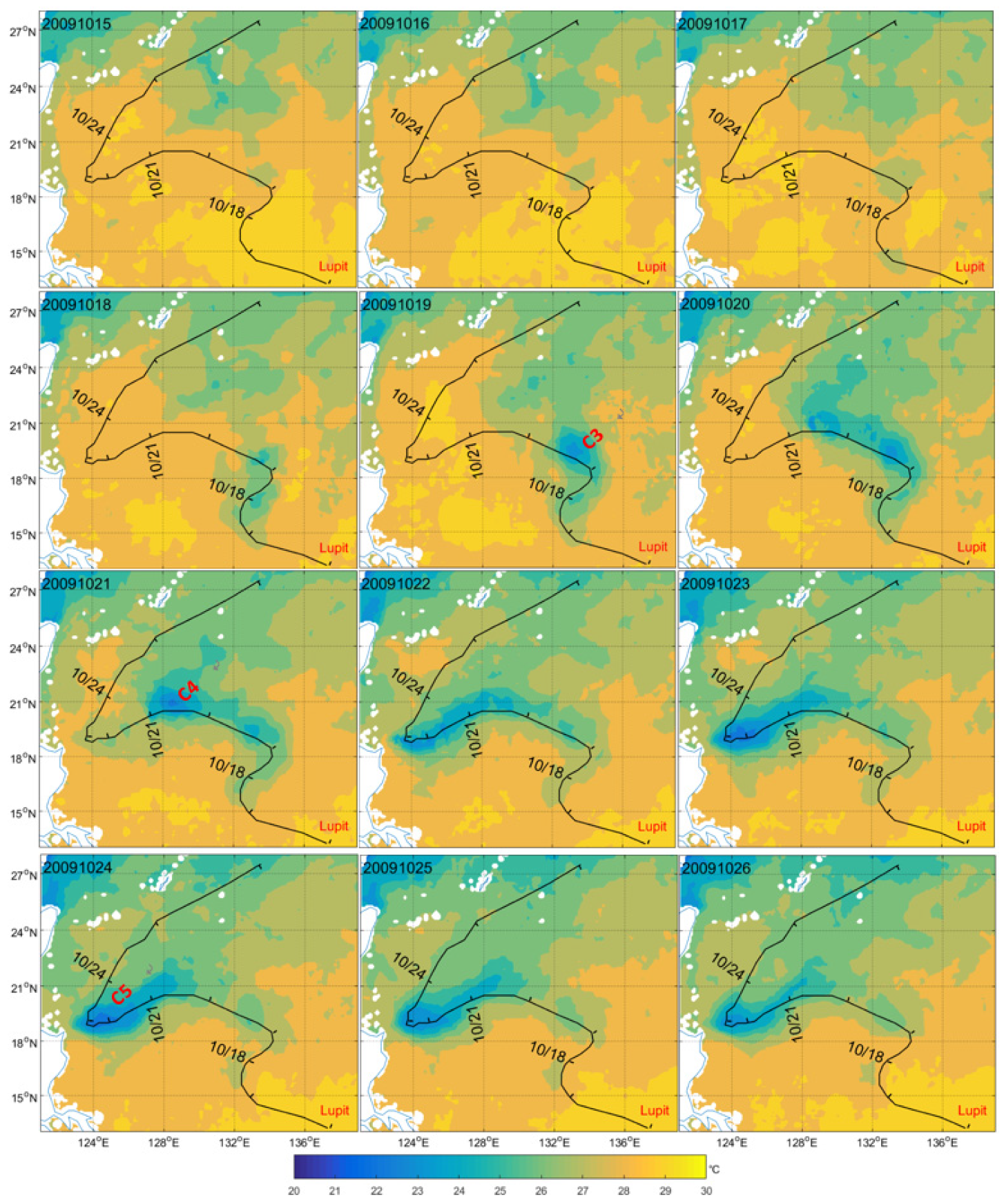
However, many SST cooling phenomena can be seen in time series of satellite-observed SST snapshots [13,38,39]. For example, Figure 1 shows the daily SST fields during the super-typhoon Lupit (2009). However, quantitative methods are required to evaluate SST cooling in many applications [20,40,41], including the heat content [42,43,44], the sea surface height [31,45], the mixed layer depth [23,46,47], the surface chlorophyll-a concentration [48,49,50,51,52], and upper ocean currents [53,54,55,56,57].
In order to quantitatively measure the SST cooling response, we need to calculate the difference between the pre-typhoon and post-typhoon SST fields. Two quantitative methods are currently used to evaluate SST cooling. The averaged difference response (ADR) method averages the SST fields two or three days pre- and post-typhoon and then evaluates the SST cooling response with the average SST fields [19,58]. The domain maximum response (DMR) method uses daily SST snapshots to calculate the SST difference field and then identifies the day with the maximum SST cooling [59,60,61,62,63].
Although both the ADR and DMR methods can quantitatively calculate SST cooling, neither can accurately evaluate the SST cooling field, especially for long-lasting typhoons where there are large changes in SST caused by natural forcing. For example, SST cooling evaluated by the ADR method is weaker than the actual value as a result of smoothing and some SST cooling centers may disappear, especially for rapidly cooling/recovering centers (e.g., C4 in Figure 1) and weak cooling centers (e.g., C3 in Figure 1). Although the DMR method can identify the maximum cooling center (e.g., C5 in Figure 1), other cooling centers (e.g., C3 and C4 in Figure 1) might be missed because only a single figure is used. This might be more significant when the typhoon has a meandering, lingering track with sharp turns—for example, the other cooling centers (e.g., C3 and C4 in Figure 1) are not seen in Figure 2b. Other typhoons may be passing the same or nearby region [60,64]. The response of the ocean is then a combination of forcing by these single typhoons and is difficult to distinguish by these methods, which could be incorrect in these complex environments.
The main reason why neither the ADR nor the DMR method can accurately calculate the SST response is because the SST fields are synchronized with respect to time in both methods. However, the time at which forcing by the typhoon starts varies with location, as does the time when the SST drops (see Figure 2d). It is clear that the SST drops as a result of typhoon forcing. To accurately calculate the response of the SST, we need to consider the evolution of the SST forced by the typhoon over time for each grid location, rather than choosing a synchronous time for the SST response over the entire study domain. We report here a new method, the grid-based maximum response (GMR) method, which uses asynchronous SST fields to accurately evaluate the SST cooling response.
2. Data, Study Area and Typhoons
2.1. Data
We used the merged microwave and infrared daily SST products from Remote Sensing Systems (www.remss.com), which have a spatial resolution of 9 × 9 km. The MW_IR_OI data products used included the TRMM microwave imager (TMI), advanced microwave scanning radiometer (AMSR), WindSat polarimetric radiometer and GMI measured SST data. The spatial resolution of the SST retrieval is limited by the ratio of the radiation wavelength to the antenna diameter and by the satellite altitude. For TMI, the spatial resolution is about 50 km. This relatively coarse resolution is the major limitation of microwave SST retrievals as compared to infrared retrievals. In order to improve the resolution, the dataset also included the SST data detected in the infrared band by the moderate-resolution imaging spectroradiometer (MODIS) onboard the Terra and Aqua satellites of the Earth Observation Satellite series and the visible/infrared imaging radiometer suite (VIIRS) onboard the Suomi National Polar-orbiting Partnership (S-NPP), which have higher resolutions of 1–10 km. These instruments are suitable for analyzing the response of the upper ocean to the passage of typhoons because microwave imagers and radiometers are able to penetrate clouds and the infrared channel of radiometers onboard polar-orbiting satellites has a high spatial resolution. We obtained typhoon track data, including time series data for the location of the center of the typhoon, the central pressure, and the maximum sustained wind speed at 6-h intervals, from the Joint Typhoon Warning Center (www.usno.navy.mil/JTWC/).
2.2. Study Area and Typhoons
The northwest Pacific Ocean is the world’s most active area for typhoons [65], generating about one-third of all typhoons. We considered two typical typhoons: Typhoon Lupit (2009) and Typhoon Megi (2016). Typhoon Lupit was a fast-developing typhoon that formed as a tropical storm on 14 October 2009 and then quickly strengthened into a category 5 typhoon on 19 October, before eventually dissipating on 27 October 2009. During its 14-day lifespan, Typhoon Lupit had an irregular track with an S-shaped turn [36]. Typhoon Megi was the second in a sequence of three typhoons (Malakas, Megi and Chaba), the tracks of which overlapped. We also investigated the SST cooling induced by typical super-typhoons over a 15-year period from 2004 to 2018.
3. Grid-Based Maximum Response Method
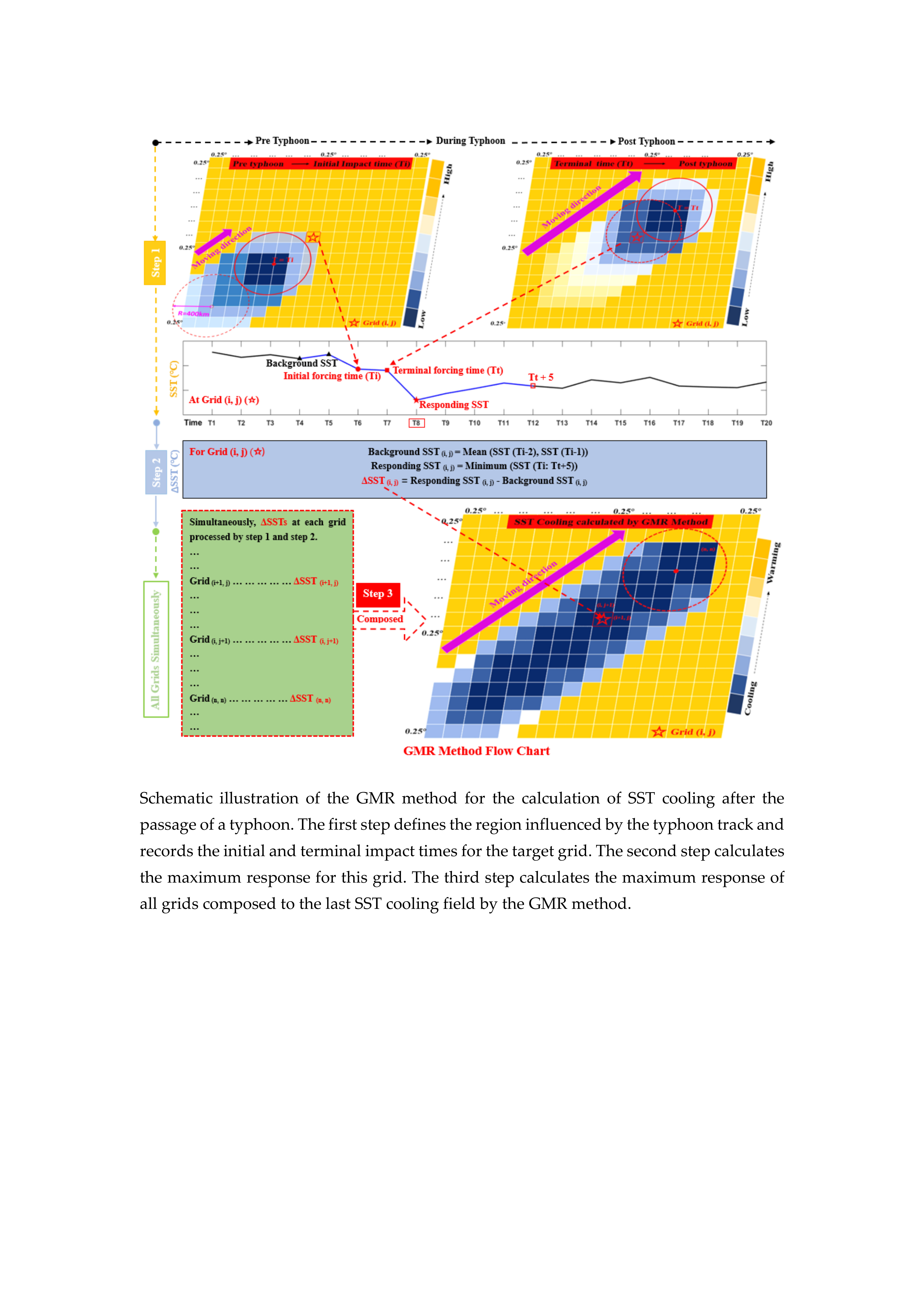
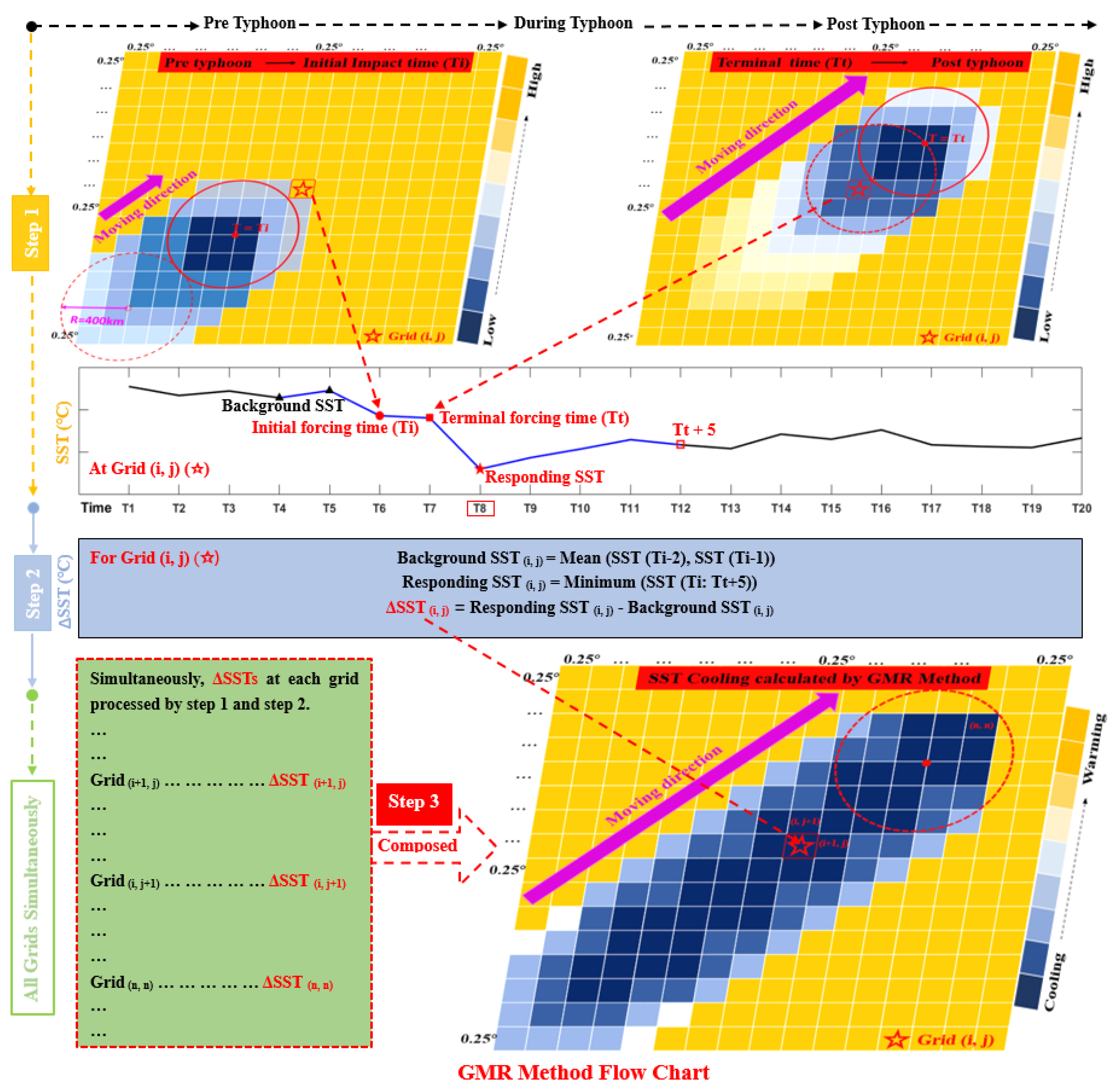
The time at which forcing by the typhoon starts varies with location, as does the time when the SST drops. We therefore developed a GMR method that uses asynchronous SST fields to accurately evaluate the cooling response of the SST. Figure 3 is a schematic illustration of the three steps in the GMR method.
The region influenced by the track of the typhoon and the corresponding critical times are defined in the first step. This region is the set of grids within 400 km of the typhoon track [32,66,67]. The SST time sequence is recorded for each grid. There are two critical times: the initial (terminal) forcing time when the typhoon enters (leaves) this region for the first (last) time. Both times may be on the same day if the translation speed of the typhoon is fast. We use the initial forcing time to determine the start time of the SST response, which is two days before the initial forcing time (Ti − 2). The terminal forcing time is used to determine the end time of the SST response, which is five days after the terminal forcing time (Tt + 5). This time was chosen because the maximum decrease in SST in previous studies rarely occurred more than five days after the passage of the typhoon [63,66,67,68]. The SST response period is defined as the period from the start time (Ti − 2) to the end time (Tt + 5), and the time of undisturbed background is also included in this period.
We calculate the background SST in the second step by averaging the SSTs from time (Ti − 2) to (Ti − 1). Some earlier studies defined the background SST as the SST on a specific day just before Ti [28,36,45]. The responding SST is calculated by finding the minimum SST within the time period Ti to (Tt + 5). The cooling of the SST in this grid is then calculated as responding SST minus the background SST.
In the third step, the SST cooling response in each grid is plotted in a new map, with both the minimum SST and the corresponding date recorded in each grid. The maximum response in all grids in the domain influenced by the typhoon is shown as the last SST cooling field. The resulting map is the SST cooling map obtained by the GMR method; a map of the corresponding dates can also be obtained.
Our method is slightly more complex than the ADR and DMR methods and used three artificial parameters: the 400 km distance, the five-day response duration, and the two-day pre-typhoon average, which are discussed in the Section 5. However, the additional work is worth it.
4. Results
4.1. Typhoon Lupit
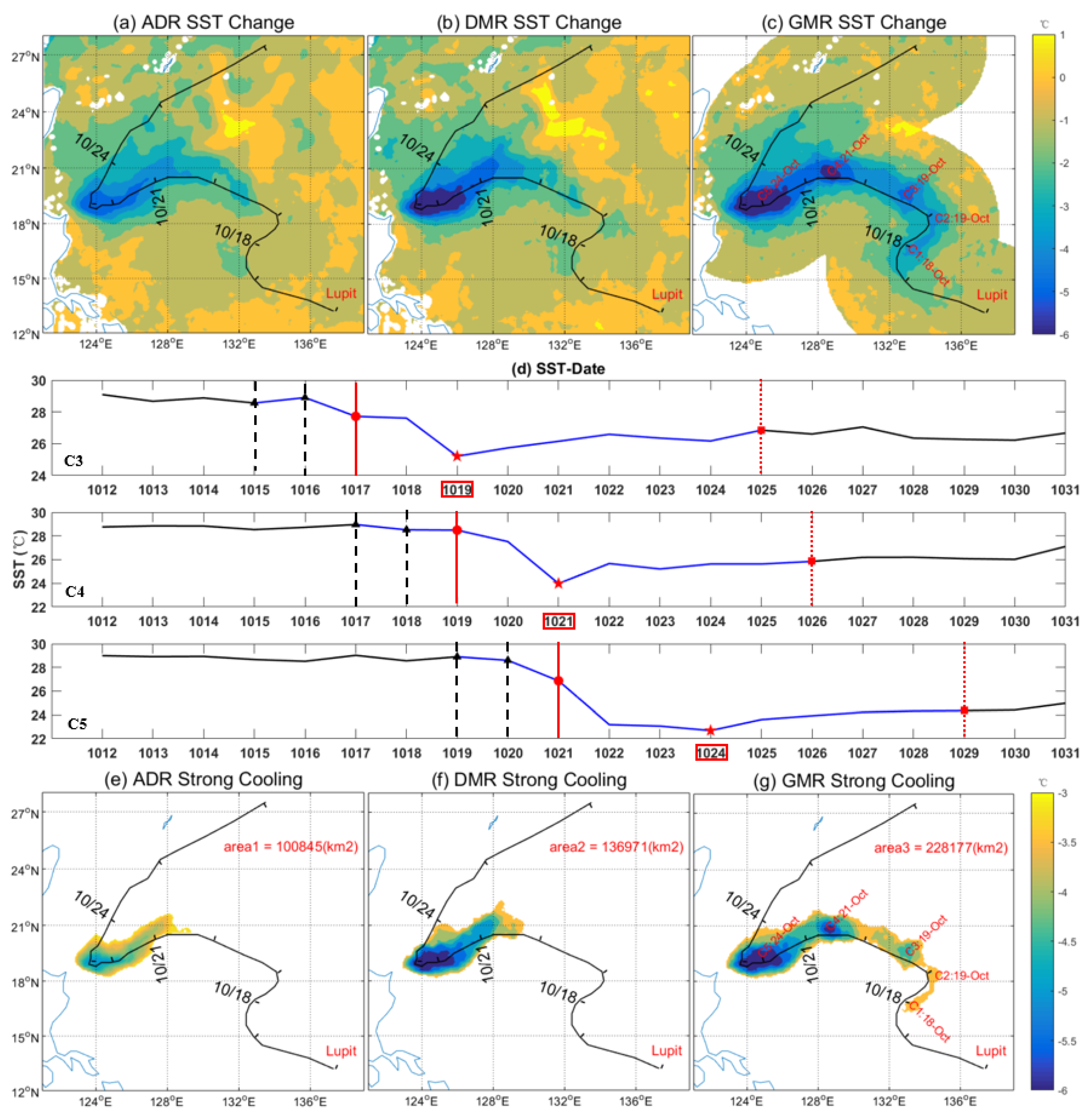
Figure 2a shows the SST response field after Typhoon Lupit obtained using the ADR method. The SST cooling is smooth with a maximum cooling temperature of 5.03 °C. Figure 2b shows the SST cooling field obtained using the DMR method by choosing 24 October as the fixed maximum cooling day, in which a clear cold patch with a maximum cooling temperature of 6.34 °C is seen at the location of the S-shaped turn on 22 October. Figure 2c shows the SST response field calculated using the GMR method. There are five cooling centers (C1–C5) in the time sequence for Typhoon Lupit and the SST evolution of cooling centers C3, C4 and C5 are shown in Figure 2d. The blue segment represents the SST response period at C3, C4, and C5. The initial forcing times are shown as solid red lines in Figure 2d and occurred on 17, 19, and 21 October at C3, C4 and C5, respectively. The red dashed line represents the end of the SST response (five days after the terminal forcing time) on 25, 26, and 29 October at C3, C4, and C5, respectively. The maximum amplitudes of SST cooling are shown by the red stars and red boxes on 19, 21, and 24 October for C3, C4, and C5, respectively (Figure 2d).
The GMR method has a number of advantages over the ADR (Figure 2a) and DMR (Figure 2b) methods and shows more pronounced SST cooling. Figure 2c shows five cooling centers along the track of Typhoon Lupit where the local maximum SST cooling occurred. By contrast, the ADR and DMR methods only showed a single cooling center (C5). The maximum SST cooling of 6.36 °C at C5 is significantly larger than that of 5.03 °C obtained by the ADR method, but is similar to the cooling of 6.34 °C obtained by the DMR method. In order to eliminate the disturbance and noise in the SST response, Figure 2e–g shows the regions calculated by the ADR, DMR, and GMR methods in which SST cooling was >3 °C [30]. The areas of the regions of strong cooling calculated by the ADR, DMR and GMR methods are 100,845, 136,971, and 228,177 km2, respectively. Only two centers (C4 and C5) were covered in the ADR and DMR methods, about half of the area of strong cooling. The C1–C3 cooling centers were too weak to be captured by the ADR and DMR methods. The GMR method can therefore identify larger and more significant regions of SST cooling than the ADR and DMR methods.
In addition, the GMR method can also give more details of the SST cooling. The GMR method identified the cooling center C4, which was totally covered by cooling center C5 in both the ADR and DMR methods (Figure 2a,b). The daily SST on 21 October (Figure 1) and the SST time series (Figure 2d) show that C4 cooled rapidly on 21 October and then recovered on 22 October. This rapid SST cooling was only captured by the GMR method because the date of maximum cooling (21 October) at C4 is three days before the date of maximum cooling (24 October) at C5. The GMR method is useful for rapid SST cooling events and for regions with weaker cooling but longer cooling times (e.g., cooling centers C1, C2, and C3). These cooling centers are very weak in the ADR and DMR methods and might be ignored. However, our new method shows that they are both large and significant (Figure 2g) and their cooling period might last longer than several weeks.
4.2. Typhoon Megi
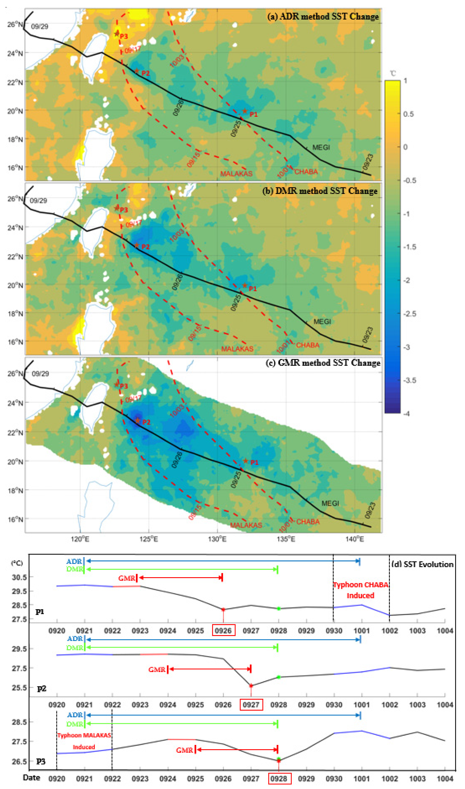
Sequential typhoons are often generated in the northwest Pacific Ocean and there have been many studies of the influence of binary typhoons on the ocean environment [64]. In general, binary (or more) typhoons have a stronger impact on the upper ocean environment, but it is difficult to separate the influence of the individual typhoons and to calculate the influence of a single target typhoon on the upper ocean. There were three sequential typhoons in 2016 (Malakas, Megi, and Chaba) and we used the second of these, Typhoon Megi, in this work. We compared the response of the SST to Typhoon Megi calculated by the ADR, DMR, and GMR methods.
Figure 4a–c shows the SST response field evaluated by ADR, DMR, and GMR methods for Typhoon Megi. We focus on the three points P1, P2, and P3, which were affected by at least two of the three typhoons. Figure 4d shows the evolution of the SST at P1, P2, and P3 during the three sequential typhoons. The fixed blue and green temporal segments in Figure 4d represent the SST response time (from pre-Megi to post-Megi) and the SST response field is calculated from the post-Megi SST field minus the pre-Megi SST field in the ADR and DMR methods, respectively. The responding SSTs and background SSTs (represented by the flexible red segments) defined in the GMR method vary at three different points as the typhoon moves (Figure 4d). Typhoon Megi first influenced P1 on 24 September and Typhoon Chaba affected this area several days later on 1 October. The post-Megi SST in the ADR method was therefore affected by Typhoon Chaba (Figure 4d). As Typhoon Megi headed northwest toward Taiwan, it influenced P2 and P3 on 25 and 26 September, respectively. However, before the impact of Typhoon Megi, the antecedent Typhoon Malakas affected P2 and P3 from 17 to 19 September, which induced a 2 °C cooling of the SST at P2 and P3, which recovered slowly about one week later. The pre-Megi background SST in the ADR and DMR methods was therefore disturbed by the influence of the antecedent typhoon Malakas. By contrast, the pre-Megi background SST and the post-Megi responding SST in the GMR method varied in different places after Typhoon Megi so the influence of the antecedent typhoon and subsequent typhoon could be effectively separated.
4.3. Typhoons in the 15 Years from 2004 to 2018
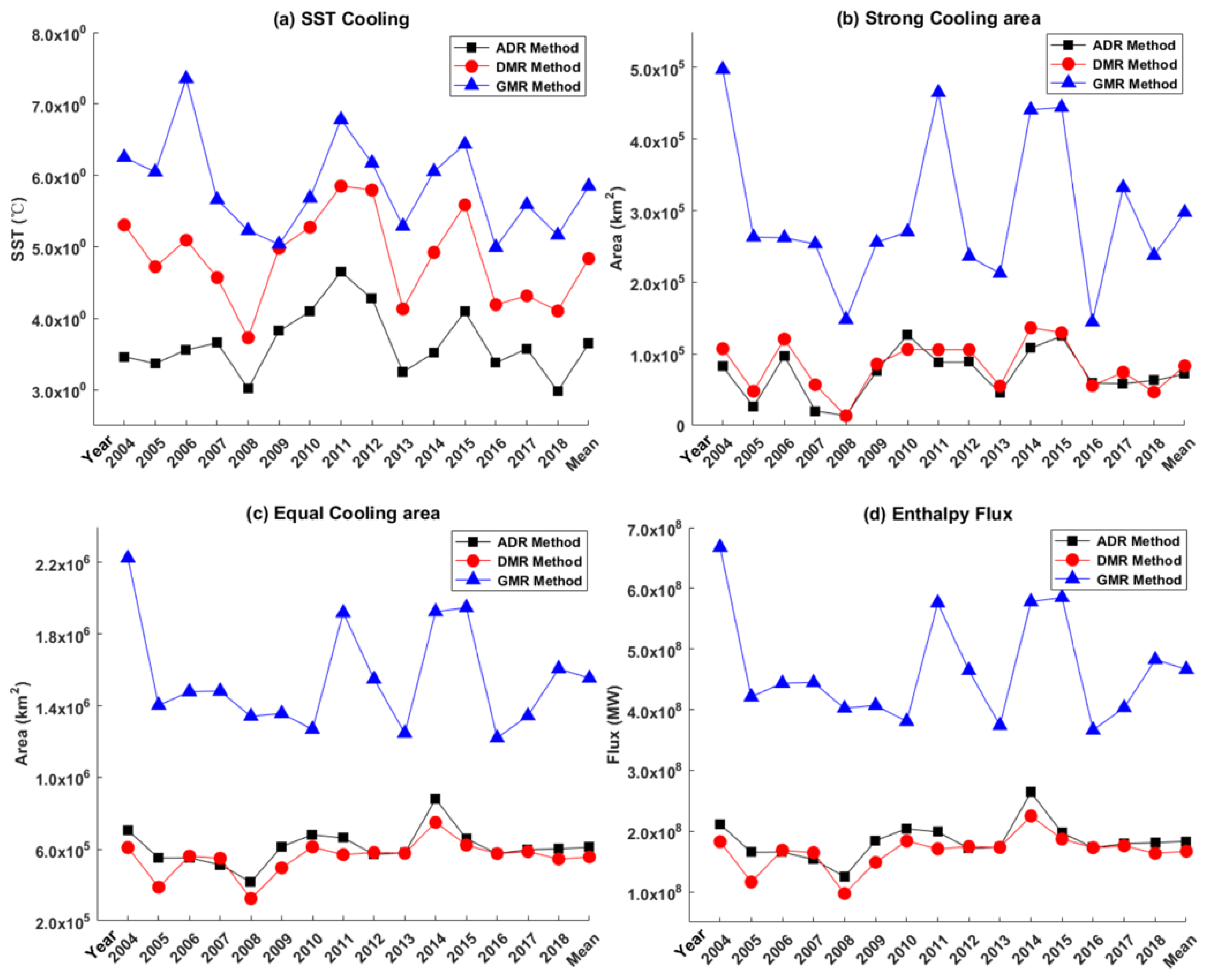
Figure 5 shows the maximum SST cooling and the area of strong cooling area from 2004 to 2018 determined using the ADR, DMR and GMR methods. The maximum SST cooling calculated by the DMR method is close to that calculated by the GMR method, whereas the maximum SST cooling calculated by the ADR method is lower (Figure 5a). The average maximum SST cooling in the time period 2004–2018 calculated by the GMR method is 5.85 °C, whereas it is 4.85 and 3.65 °C calculated by the DMR and ADR methods, respectively. The three methods show a wide variation in the area of strong cooling, especially for the typhoons with an irregular track and long-term forcing (Figure 5b). The average area of 297,500 km2 of strong SST cooling calculated by the GMR method is almost four times the areas of 71,800 and 83,100 km2 calculated by the ADR and DMR methods.
The enthalpy flux, i.e., the sensible plus latent heat fluxes, were then estimated after obtaining the SST cooling under typhoon conditions [69,70,71,72]. If the SST cooling induced by the typhoon is not sufficiently accurate, then there may be a significant error in the forecast of the typhoon track and intensity, especially for sequential typhoons. Cayan [73] observed flux anomalies of 50 W/m2 with a 0.2 °C change in SST, which suggests an enthalpy flux of 300 W/m2 for each 1 °C change in SST. Pun [74] presented a new generation of derivation to improve the forecasting of typhoons, which suggested an enthalpy flux of 100 W/m2 for each 1 °C change in SST. We calculated the cooling area equivalent to a 3 °C change in SST (Figure 5c) to obtain the enthalpy flux by the ADR, DMR, and GMR methods (Figure 5d). Our results suggest that a typhoon induces an enthalpy flux of about 4.6 × 10⁸ MW calculated by the GMR method, but an enthalpy flux of 1.7 × 10⁸ MW calculated by the ADR and DMR methods. These results accompanied with an information-modeling tracker (IMT) of tropical cyclones based on the cluster algorithm might assess the interaction of the atmosphere–ocean system [75].
5. Discussion
The above results have shown large differences between the GMR method and the previous ADR and DMR methods. To explain these differences, we compare the results of the DMR and GMR methods. The ADR method was excluded due to its similarity to the DMR method.
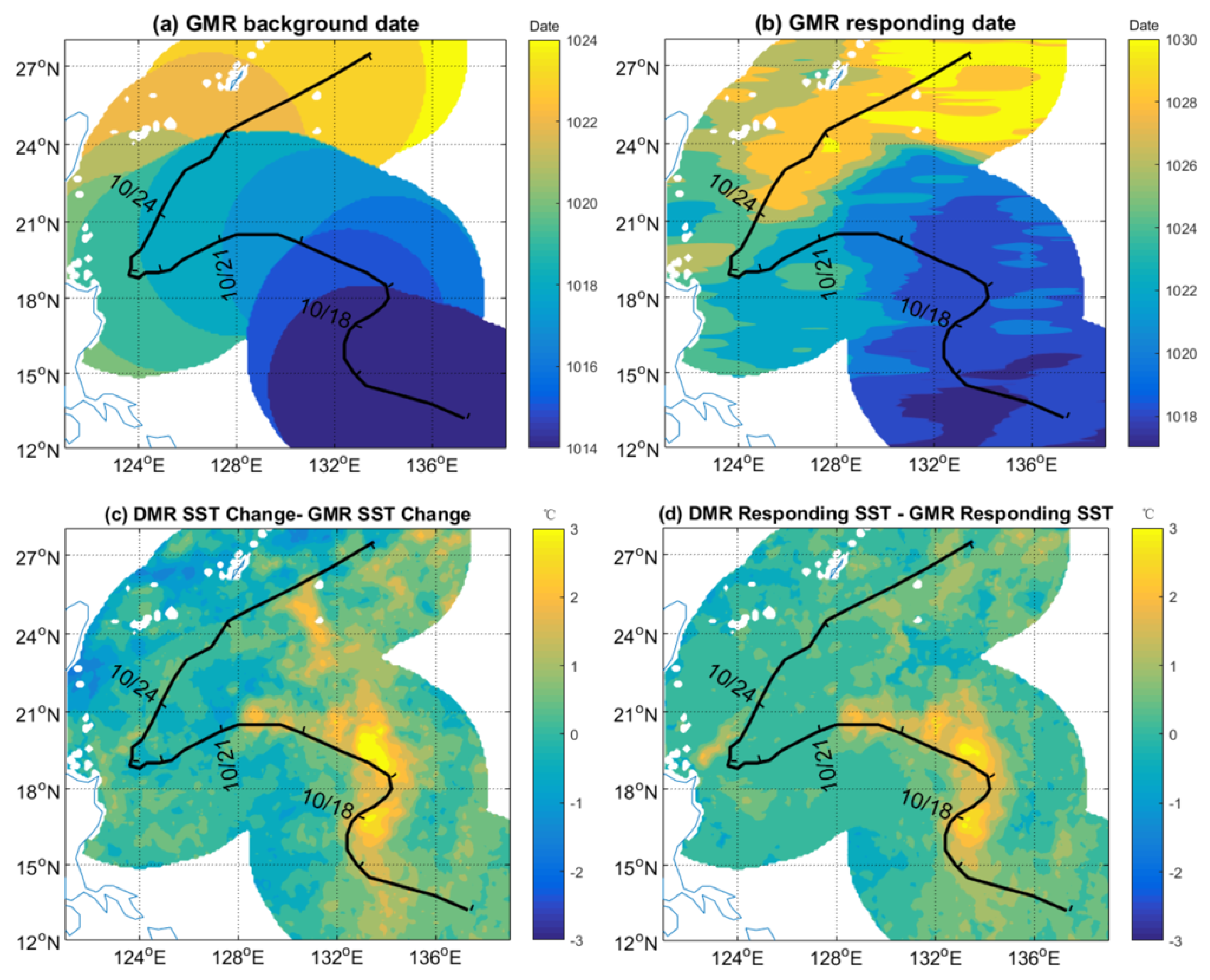
To show clearly how this difference originates, the time of background SST and the time of maximum responses derived from the GMR method are illustrated in Figure 6a,b. It is clear that the background time changes with typhoon track in Figure 6a. On the one hand, if we fixed the background time on a specific day as in the DMR method, only part of the background SST would be the same as in the GMR method. For example, if the background time was chosen as 21 October, it may suit the region with cold wakes of C4 and C5, but the SST at the region near C1 and C2 had been affected by typhoon forcing. On the other hand, if we fixed the maximum response time, the SST far behind typhoon track would recover after typhoon forcing. Both reasons will lead to underestimation of the SST cooling responses by the previous methods.
Then, we could quantitatively identify which reason is dominant. Figure 6c illustrates the difference between the GMR and DMR methods. Since we have chosen 24 October as the maximum cooling response time, the difference is smallest near the turning point on 22 October. However, the differences become larger behind the typhoon track from the cooling centers C1 to C4, especially at C3. The reason for this difference can be mainly explained by the recovery of SST after typhoon forcing. Figure 6d illustrates the SST difference between the grid-based responding date and the fixed date 24 October, which presents the SST recovery after typhoon’s passage. So, in this case, the main difference between the DMR and GMR methods is due to the recovery of SST, because the background SST was warm and seldom changed pre-typhoon’s passage. However, there might be the case that the background SST could also play an important role, e.g., when the background SST changes rapidly in winter or after sequential typhoons studied above. Moreover, although the ADR and DMR methods can calculate SST cooling response, the results in region ahead of the typhoon track (e.g., pre typhoon maximum cooling time 24 October) are invalid since the typhoon has not influenced them yet.
Important too are the setting of parameters in the GMR method. The proposed method based on satellite observations did not give consistent results and different parameters need to be used in different situations. The following issues require further study.
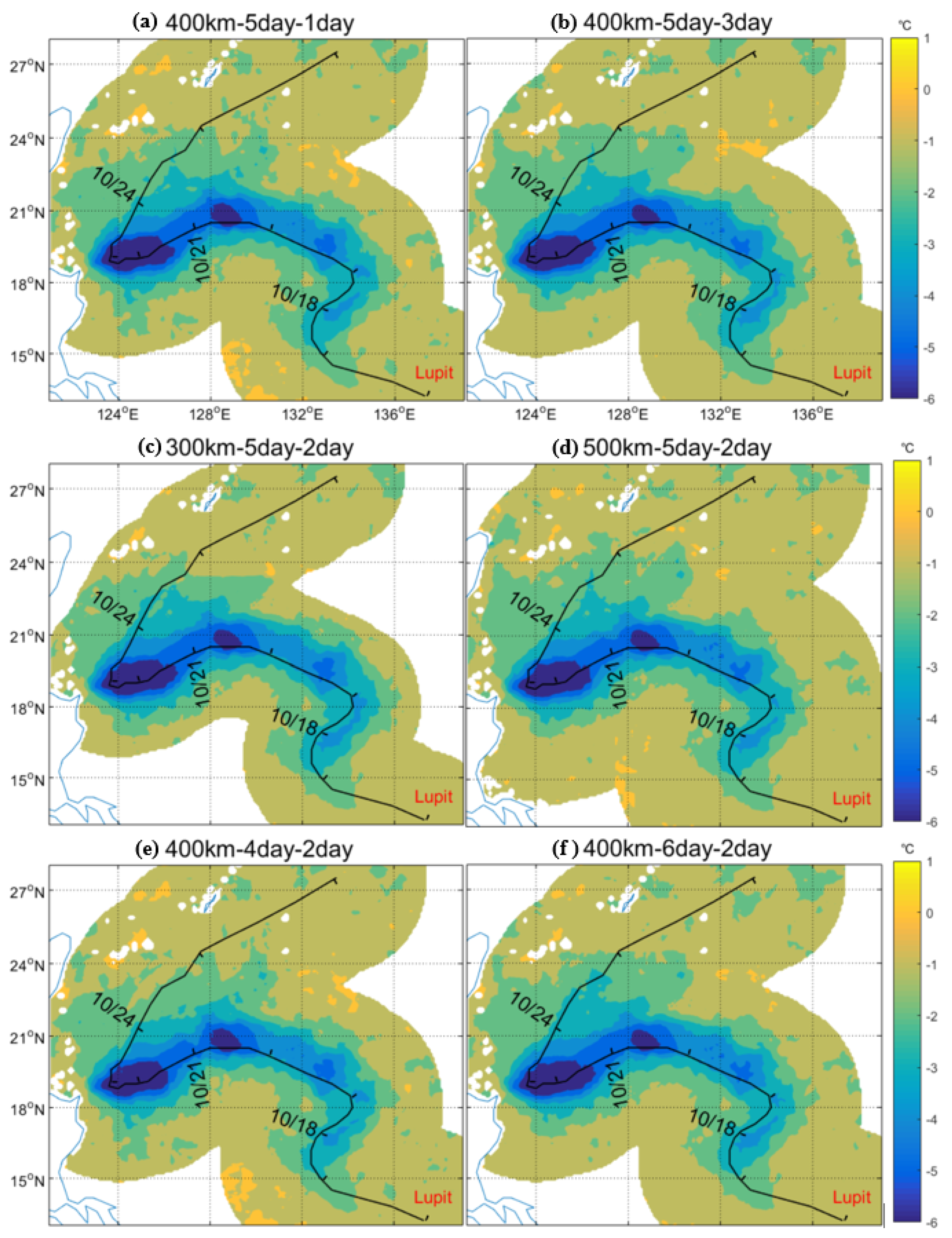
(1) Calculation of the background SST. We used the two-day average SST before the initial time that the typhoon arrived in the grid as the background SST. We could also have used the one-day (Figure 7a) or three-day (Figure 7b) average SST.
(2) The choice of typhoon radius. We selected 400 km as the radius of the three typhoons investigated in this study. The radius is an important parameter in the calculation of the initial and terminating times. We could also have used 300 km (Figure 7c) or 500 km (Figure 7d) if the typhoon was a little weaker or stronger, respectively.
(3) The choice of end time of SST response period. We chose five days after the typhoon has left the distance of 400 km for the last time as the end time. We could also have used three days (Figure 7e) or seven days (Figure 7f) if the sequential typhoons had been separated by five days or less.
We tested these different scenarios for Typhoon Lupit and compared them with the default result. In general, there was no difference between the results obtained for Typhoon Lupit using different parameters. However, we would obtain an inaccurate result if unsuitable parameters were used in particular situations. Some other details need discussion, such as the background SST dropping during the passage of typhoons in the autumn and winter. These factors need to be taken into consideration when using this new method.
6. Conclusions
We developed a new method to evaluate the response of the upper ocean to typhoon forcing. The method consists of three steps. In the first step, the initial forcing time (Ti) and the terminal forcing time (Tt) of the typhoon are recorded and the SST response period is defined as the time from the start time (Ti − 2) to the end time (Tt + 5) in each grid. In the second step, the minimum SST within the time from the initial forcing time (Ti) to the end time (Tt + 5) is chosen as the responding SST and the SST cooling is evaluated in each grid by subtracting the background SST from the responding SST. In the last step, the SST cooling response in each grid is displayed as the GMR result in a map.
Two earlier methods were compared with the new method for two typical typhoons, namely Typhoon Lupit (2009) and Typhoon Megi (2016), to show the contrast between these methods and our new method in terms of the maximum amplitude of SST cooling and the location of the SST cooling centers with the corresponding dates and presence of sequential typhoons. The GMR method captured five major cooling centers and their corresponding dates with a maximum SST cooling of 6.36 °C after the passage of Typhoon Lupit, whereas the ADR and DMR methods only captured one cooling center with a maximum SST cooling of 5.03 °C. The influence of Typhoon Megi in a series of sequential typhoons was calculated accurately by separating the influence of the earlier and later typhoons Malakas and Chaba. All the typhoons in the northwest Pacific Ocean from 2004 to 2018 were investigated using the three methods. The average maximum SST cooling calculated by the GMR, DMR, and ADR methods was 5.85, 4.85, and 3.65 °C, respectively. Each typhoon could induce a strong area of SST cooling of 297,500 km2 calculated by the GMR method, which is almost four times the areas of 71,800 and 83,100 km2 calculated by the ADR and DMR methods.
Cooling of the SST is one of the most important oceanic phenomena induced by typhoons. The accurate calculation of SST cooling is important in the quantitative evaluation of the cold wake and could improve estimates of many related phenomenon and quantities, such as the air–sea enthalpy flux, the change in intensity of the typhoon, the dissipation of the power of the typhoon, the concentration of surface chlorophyll, and the size and surface wind speed of the typhoon. We evaluated the air–sea enthalpy flux by calculating the 3 °C equivalent SST cooling area induced by the typhoon, which showed that a typhoon could induce roughly 4.6 × 10⁸ MW calculated by the GMR method, but only 1.7 × 10⁸ MW calculated by the ADR and DMR methods.
Although this new method focused on calculating SST cooling, we could also evaluate the response of other physical and biological responses to typhoons using suitable datasets, such as the sea surface salinity, the sea surface height, the mixed layer depth, and the heat content of the upper ocean. This GMR method could also be applied to research concerning the spatial distribution of the maximum SST cooling time and the re-cooling time after the passage of a typhoon, or the three-dimensional response of the ocean to a typhoon. In general, our findings have important implications for accurately estimating the response of the ocean to typhoons and their feedback in air–sea interaction systems.
Author Contributions
J.L. and L.S. conceived the original ideal, designed this study and wrote the paper; J.L. collected and analyzed the data; Y.Y. helped the result interpretation, suggested for the topic and provided comments and suggestions on the paper. H.C. assisted in manuscript preparation and revision. All authors have read and agreed to the published version of the manuscript.
Funding
This work was supported by the National Foundation of Natural Science of China (No. 41876013), the National Programme on Global Change and Air–Sea Interaction (GASI-IPOVAI-04) and open funding of State Key Laboratory of Loess and Quaternary Geology (SKLLQG1842).
Acknowledgments
We thank the anonymous reviewers for their useful comments. We also thank Remote Sensing Systems for the SST and SSW data (http://www.remss.com/), the Joint Typhoon Warning Center (JTWC) for providing typhoon track data (http://www.usno.navy.mil/JTWC/), and Archiving, Validation and Interpretation of Satellite Oceanographic for the SSHA and Geostrophic Velocity data (https://www.aviso.altimetry.fr/en/data/products/).
Conflicts of Interest
The authors declare no conflict of interest.
References
- Gray, W.M.; Brody, L.R. Global view of the origin of tropical disturbances and storms. Mon. Weather Rev. 1968, 96, 669–700. [Google Scholar] [CrossRef]
- Gray, W.M. Tropical cyclone genesis. In Department of Atmospheric Science Paper; Colorado State University: Fort Collins, CO, USA, 1975; p. 121. [Google Scholar]
- Emanuel, K.A. An air-sea interaction theory for tropical cyclones. Part I: Steady-state maintenance. J. Atmos. Sci. 1986, 43, 585–605. [Google Scholar] [CrossRef]
- Wang, G.H.; Su, J.L.; Ding, Y.H.; Chen, D.K. Tropical cyclone genesis over the south China sea. J. Mar. Syst. 2007, 68, 318–326. [Google Scholar] [CrossRef]
- Emanuel, K.A. Thermodynamic control of hurricane intensity. Nature 1999, 401, 665–669. [Google Scholar] [CrossRef]
- Schade, L.R.; Emanuel, K.A. The ocean’s effect on the intensity of tropical cyclones: Results from a simple coupled atmosphere–ocean model. J. Atmos. Sci. 1999, 56, 642–651. [Google Scholar] [CrossRef] [Green Version]
- Mei, W.; Xie, S.P.; Primeau, F.; McWilliams, J.C.; Pasquero, C. Northwestern Pacific typhoon intensity controlled by changes in ocean temperatures. Sci. Adv. 2015, 1, e1500014. [Google Scholar] [CrossRef] [PubMed] [Green Version]
- Lin, I.I.; Wu, C.C.; Pun, I.F.; Ko, D.S. Upper-ocean thermal structure and the western North Pacific category 5 typhoons. Part I: Ocean features and the category 5 typhoons’ intensification. Mon. Weather Rev. 2008, 136, 3288–3306. [Google Scholar] [CrossRef] [Green Version]
- Emanuel, K. Tropical cyclones. Annu. Rev. Earth Planet Sci. 2003, 31, 75–104. [Google Scholar] [CrossRef]
- McClain, E.P.; Pichel, W.G.; Walton, C.C. Comparative performance of AVHRR-based multichannel sea surface temperatures. J. Geophys. Res. Oceans 1985, 90, 11587–11601. [Google Scholar] [CrossRef]
- Monaldo, F.M.; Sikora, T.D.; Babin, S.M.; Sterner, R.E. Satellite imagery of sea surface temperature cooling in the wake of Hurricane Edouard (1996). Mon. Wea. Rev. 1997, 125, 2716–2721. [Google Scholar] [CrossRef]
- Black, P.G.; Holland, G.J. The boundary layer of tropical cyclone Kerry (1979). Mon. Weather Rev. 1995, 123, 2007–2028. [Google Scholar] [CrossRef] [Green Version]
- Wentz, F.J.; Gentemann, C.; Smith, D.; Chelton, D. Satellite measurements of sea surface temperature through clouds. Science 2000, 288, 847–850. [Google Scholar] [CrossRef] [PubMed] [Green Version]
- Hazelworth, J.B. Water temperature variations resulting from hurricanes. J. Geophys. Res. 1968, 73, 5105–5123. [Google Scholar] [CrossRef]
- Shay, L.K.; Black, P.G.; Mariano, A.J.; Hawkins, J.D.; Elsberry, R.L. Upper ocean response to Hurricane Gilbert. J. Geophys. Res. 1992, 97, 20227. [Google Scholar] [CrossRef] [Green Version]
- Wang, G.; Wu, L.; Johnson, N.C.; Ling, Z. Observed three-dimensional structure of ocean cooling induced by Pacific tropical cyclones. Geophys. Res. Lett. 2016, 43, 7632–7638. [Google Scholar] [CrossRef]
- Zhang, H.; Chen, D.; Zhou, L.; Liu, X.; Ding, T.; Zhou, B. Upper ocean response to typhoon Kalmaegi (2014). J. Geophys. Res. Oceans 2016, 121, 6520–6535. [Google Scholar] [CrossRef]
- Stramma, L.; Cornillon, P.; Price, J.F. Satellite observations of sea surface cooling by hurricanes. J. Geophys. Res. 1986, 91, 5031. [Google Scholar] [CrossRef]
- Cornillon, P.; Stramma, L.; Price, J.F. Satellite measurements of sea surface cooling during hurricane Gloria. Nature 1987, 326, 373–375. [Google Scholar] [CrossRef] [Green Version]
- Lin, I.I.; Liu, W.T.; Wu, C.C.; Chiang, J.C.H.; Sui, C.H. Satellite observations of modulation of surface winds by typhoon-induced upper ocean cooling. Geophys. Res. Lett. 2003, 30, 1131. [Google Scholar] [CrossRef]
- Leipper, D.F. Observed ocean conditions and Hurricane Hilda, 1964. J. Atmos. Sci. 1967, 24, 182–186. [Google Scholar] [CrossRef] [Green Version]
- Brand, S. The effects on a tropical cyclone of cooler surface waters due to upwelling and mixing produced by a prior tropical cyclone. J. Appl. Meteorol. 1971, 10, 865–874. [Google Scholar] [CrossRef] [Green Version]
- Price, J.F. Upper Ocean Response to a Hurricane. J. Phys. Oceanogr. 1981, 11, 153–175. [Google Scholar] [CrossRef] [Green Version]
- Lin, I.I.; Black, P.; Price, J.F.; Yang, C.Y.; Chen, S.S. An ocean coupling potential intensity index for tropical cyclones. Geophys. Res. Lett. 2013, 40, 1878–1882. [Google Scholar] [CrossRef]
- Khain, A.P.; Ginis, I.D. The mutual response of a moving tropical cyclone and the ocean. Beitr. Phys. Atmos. 1991, 64, 125–142. [Google Scholar]
- Vecchi, G.A.; Soden, B.J. Effect of remote sea surface temperature change on tropical cyclone potential intensity. Nature 2007, 450, 1066–1070. [Google Scholar] [CrossRef]
- Holland, G.J. The maximum potential intensity of tropical cyclones. J. Atmos. Sci. 1997, 54, 2519–2541. [Google Scholar] [CrossRef]
- Mei, W.; Lien, C.C.; Lin, I.I.; Xie, S.P. Tropical cyclone–induced ocean response: A comparative study of the South China Sea and tropical northwest Pacific. J. Clim. 2015, 28, 5952–5968. [Google Scholar] [CrossRef]
- Zhang, J.; Lin, Y.; Chavas, D.R.; Mei, W. Tropical cyclone cold wake size and its applications to power dissipation and ocean heat uptake estimates. Geophys. Res. Lett. 2019, 46, 10177–10185. [Google Scholar] [CrossRef]
- Walker, N.D.; Leben, R.R.; Balasubramanian, S. Hurricane-forced upwelling and chlorophylla enhancement within cold-core cyclones in the Gulf of Mexico. Geophys. Res. Lett. 2005, 32, L18610. [Google Scholar] [CrossRef]
- Sun, L.; Yang, Y.J.; Xian, T.; Lu, Z.; Fu, Y.F. Strong enhancement of chlorophyll a concentration by a weak typhoon. Mar. Ecol. Prog. Ser. 2010, 404, 39–50. [Google Scholar] [CrossRef]
- Babin, S.M.; Carton, J.A.; Dickey, T.D.; Wiggert, J.D. Satellite evidence of hurricane-induced phytoplankton blooms in an oceanic desert. J. Geophys. Res. Oceans 2004, 109, C03043. [Google Scholar] [CrossRef]
- Shang, S.; Li, L.; Sun, F.; Wu, J.; Hu, C.; Chen, D.; Ning, X.; Qiu, Y.; Zhang, C.; Shang, S. Changes of temperature and bio-optical properties in the South China Sea in response to Typhoon Lingling, 2001. Geophys. Res. Lett. 2008, 35, L10602. [Google Scholar] [CrossRef] [Green Version]
- Liu, S.; Li, J.; Sun, L.; Wang, G.; Tan, D.; Huang, P.; Yan, H.; Gao, S.; Liu, C.; Gao, Z.; et al. Basin-wide responses of the South China Sea environment to Super Typhoon Mangkhut (2018). Sci. Total Environ. 2020, 731, 139093. [Google Scholar] [CrossRef]
- Zhao, H.; Wang, Y. Phytoplankton increases induced by tropical cyclones in the South China Sea during 1998–2015. J. Geophys. Res. Oceans 2018, 123, 2903–2920. [Google Scholar] [CrossRef]
- Cheung, H.F.; Pan, J.Y.; Gu, Y.Z.; Wang, Z.Z. Remote-sensing observation of ocean responses to Typhoon Lupit in the northwest Pacific. Int. J. Remote Sens. 2012, 34, 1478–1491. [Google Scholar] [CrossRef]
- Lin, Y.; Zhao, M.; Zhang, M. Tropical cyclone rainfall area controlled by relative sea surface temperature. Nat. Commun. 2015, 6, 1–7. [Google Scholar] [CrossRef] [PubMed]
- Siswanto, E.; Ishizaka, J.; Morimoto, A.; Tanaka, K.; Okamura, K.; Kristijono, A.; Saino, T. Ocean physical and biogeochemical responses to the passage of Typhoon Meari in the East China Sea observed from Argo float and multiplatform satellites. Geophys. Res. Lett. 2008, 35, L15604. [Google Scholar] [CrossRef]
- Wu, C.R.; Chang, Y.L.; Oey, L.Y.; Chang, C.W.J.; Hsin, Y.C. Air-sea interaction between tropical cyclone Nari and Kuroshio. Geophys. Res. Lett. 2008, 35, L12605. [Google Scholar] [CrossRef]
- Sriver, R.L.; Huber, M. Observational evidence for an ocean heat pump induced by tropical cyclones. Nature 2007, 447, 577–580. [Google Scholar] [CrossRef]
- Sun, L.; Li, Y.X.; Yang, Y.J.; Wu, Q.; Chen, X.T.; Li, Q.Y.; Li, Y.B.; Xian, T. Effects of super typhoons on cyclonic ocean eddies in the western North Pacific: A satellite data-based evaluation between 2000 and 2008. J. Geophys. Res. Oceans 2014, 119, 5585–5598. [Google Scholar] [CrossRef]
- Mei, W.; Pasquero, C. Spatial and temporal characterization of sea surface temperature response to tropical cyclones. J. Clim. 2013, 26, 3745–3765. [Google Scholar] [CrossRef]
- Cheng, L.; Zhu, J.; Sriver, R.L. Global representation of tropical cyclone-induced short-term ocean thermal changes using Argo data. Ocean Sci. 2015, 11, 719–741. [Google Scholar] [CrossRef] [Green Version]
- Zhang, H.; Wu, R.H.; Chen, D.K.; Liu, X.H.; He, H.L.; Tang, Y.M.; Ke, D.X.; Shen, Z.Q.; Li, J.D.; Xie, J.C.; et al. Net Modulation of Upper Ocean Thermal Structure by Typhoon Kalmaegi (2014). J. Geophys. Res. Oceans 2018, 123, 7154–7171. [Google Scholar] [CrossRef]
- Zheng, Z.W.; Ho, C.R.; Kuo, N.J. Importance of pre-existing oceanic conditions to upper ocean response induced by Super Typhoon Hai-Tang. Geophys. Res. Lett. 2008, 35, L20603. [Google Scholar] [CrossRef]
- Sun, L.; Yang, Y.J.; Xian, T.; Wang, Y.; Fu, Y.F. Ocean Responses to Typhoon Namtheun Explored with Argo Floats and Multiplatform Satellites. Atmosphere-Ocean 2012, 50, 15–26. [Google Scholar] [CrossRef] [Green Version]
- Pan, J.Y.; Sun, Y.J. Estimate of Ocean Mixed Layer Deepening after a Typhoon Passage over the South China Sea by Using Satellite Data. J. Phys. Oceanogr. 2013, 43, 498–506. [Google Scholar] [CrossRef]
- Lin, I.; Liu, W.T.; Wu, C.C.; Wong, G.T.F.; Hu, C.; Chen, Z.; Liang, W.D.; Yang, Y.; Liu, K.K. New evidence for enhanced ocean primary production triggered by tropical cyclone. Geophys. Res. Lett. 2003, 30, 1718. [Google Scholar] [CrossRef] [Green Version]
- Pan, J.; Huang, L.; Devlin, A.T.; Lin, H. Quantification of typhoon-induced phytoplankton blooms using satellite multi-sensor data. Remote Sens. 2018, 10, 318. [Google Scholar] [CrossRef] [Green Version]
- Liu, Y.; Tang, D.; Evgeny, M. Chlorophyll concentration response to the typhoon wind-pump induced upper ocean processes considering air–sea heat exchange. Remote Sens. 2019, 11, 1825. [Google Scholar] [CrossRef] [Green Version]
- Zhao, H.; Tang, D.; Wang, D. Phytoplankton blooms near the Pearl River estuary induced by Typhoon Nuri. J. Geophys. Res. Oceans 2009, 114, C12027. [Google Scholar] [CrossRef]
- Chen, Y.; Tang, D. Eddy-feature phytoplankton bloom induced by a tropical cyclone in the South China Sea. Int. J. Remote Sens. 2012, 33, 7444–7457. [Google Scholar] [CrossRef]
- Yang, Y.J.; Sun, L.; Liu, Q.; Xian, T.; Fu, Y.F. The biophysical responses of the upper ocean to the typhoons Namtheun and Malou in 2004. Int. J. Remote Sens. 2010, 31, 4559–4568. [Google Scholar] [CrossRef]
- Yue, X.; Zhang, B.; Liu, G.; Li, X.; Zhang, H.; He, Y. Upper ocean response to typhoon Kalmaegi and Sarika in the South China Sea from multiple-satellite observations and numerical simulations. Remote Sens. 2018, 10, 348. [Google Scholar] [CrossRef] [Green Version]
- Zhang, H.; Liu, X.; Wu, R.; Liu, F.; Yu, L.; Shang, X.; Qi, Y.; Wang, Y.; Song, X.; Xie, X.; et al. Ocean Response to Successive Typhoons Sarika and Haima (2016) Based on Data Acquired via Multiple Satellites and Moored Array. Remote Sens. 2019, 11, 2360. [Google Scholar] [CrossRef] [Green Version]
- Wang, G.; Ling, Z.; Wang, C. Influence of tropical cyclones on seasonal ocean circulation in the South China Sea. J. Geophys. Res. Oceans 2019, 114, C10022. [Google Scholar] [CrossRef] [Green Version]
- Liu, S.S.; Sun, L.; Wu, Q.; Yang, Y.J. The responses of cyclonic and anticyclonic eddies to typhoon forcing: The vertical temperature-salinity structure changes associated with the horizontal convergence/divergence. J. Geophys. Res. Oceans 2017, 122, 4974–4989. [Google Scholar] [CrossRef]
- Sakaida, F.; Kawamura, H.; Toba, Y. Sea surface cooling caused by typhoons in the Tohoku area in August 1989. J. Geophys. Res. Oceans 1998, 103, 1053–1065. [Google Scholar] [CrossRef]
- Chu, P.C.; Veneziano, J.M.; Fan, C.; Carron, M.J.; Liu, W.T. Response of the South China Sea to tropical cyclone Ernie 1996. J. Geophys. Res. Oceans 2000, 105, 13991–14009. [Google Scholar] [CrossRef] [Green Version]
- Wu, R.H.; Li, C.Y. Upper ocean response to the passage of two sequential typhoons. Deep Sea Res. Part I 2018, 132, 68–79. [Google Scholar] [CrossRef]
- Yu, S.Y.; Subrahmanyam, M.V. Typhoon-Induced SST Cooling and Rainfall Variations: The Case of Typhoon CHAN-HOM and Nangka. Open Access Libr. J. 2017, 4, 1–12. [Google Scholar]
- Tsai, Y.; Chern, C.S.; Wang, J. Typhoon induced upper ocean cooling off northeastern Taiwan. Geophys. Res. Lett. 2008, 35, L14605. [Google Scholar] [CrossRef]
- Shi, Y.X.; Xie, L.L.; Zheng, Q.A.; Zhang, S.W.; Li, M.M.; Li, J.Y. Unusual coastal ocean cooling in the northern South China Sea by a katabatic cold jet associated with Typhoon Mujigea (2015). Acta Oceanol. Sin. 2019, 38, 62–75. [Google Scholar] [CrossRef]
- Yang, Y.J.; Sun, L.; Duan, A.M.; Li, Y.B.; Fu, Y.F.; Yan, Y.F.; Wang, Z.Q.; Xian, T. Impacts of the binary typhoons on upper ocean environments in November 2007. J. Appl. Remote Sens. 2012, 6, 063583. [Google Scholar] [CrossRef]
- Chen, D.K.; Lei, X.; Wang, W.; Wang, G.; Han, G.; Zhou, L. Upper ocean response and feedback mechanisms to typhoon. Adv. Earth Sci. 2013, 28, 1077–1086. [Google Scholar]
- Elsberry, R.L.; Fraim, T.S.; Trapnell, R.N., Jr. A mixed layer model of the oceanic thermal response to hurricanes. J. Geophys. Res. 1976, 81, 1153–1162. [Google Scholar] [CrossRef]
- Price, J.F.; Morzel, J.; Niiler, P.P. Warming of SST in the cool wake of a moving hurricane. J. Geophys. Res. 2008, 113, C07010. [Google Scholar] [CrossRef] [Green Version]
- Dare, R.A.; McBride, J.L. Sea surface temperature response to tropical cyclones. Mon. Weather Rev. 2011, 139, 3798–3808. [Google Scholar] [CrossRef]
- Cione, J.J.; Uhlhorn, E.W. Sea surface temperature variability in hurricanes: Implications with respect to intensity change. Mon. Weather Rev. 2003, 131, 1783–1796. [Google Scholar] [CrossRef] [Green Version]
- Jacob, S.D.; Shay, L.K. The role of oceanic mesoscale features on the tropical cyclone–induced mixed layer response: A case study. J. Phys. Oceanogr. 2003, 33, 649–676. [Google Scholar] [CrossRef]
- Black, P.G.; D’Asaro, E.A.; Drennan, W.M.; French, J.R.; Niiler, P.P.; Sanford, T.B.; Terrill, E.J.; Walsh, E.J.; Zhang, J.A. Air-sea exchange in hurricanes: Synthesis of observations from the coupled boundary layer air–sea transfer experiment. Bull. Am. Meteorol. Soc. 2007, 88, 357–374. [Google Scholar] [CrossRef] [Green Version]
- Lin, I.I.; Pun, I.F.; Wu, C.C. Upper-ocean thermal structure and the western North Pacific category 5 typhoons. Part II: Dependence on translation speed. Mon. Weather Rev. 2009, 137, 3744–3757. [Google Scholar] [CrossRef]
- Cayan, D.R. Latent and sensible heat flux anomalies over the northern oceans: Driving the sea surface temperature. J. Phys. Oceanogr. 1992, 22, 859–881. [Google Scholar] [CrossRef]
- Pun, I.F.; Lin, I.I.; Ko, D.S. New generation of satellite-derived ocean thermal structure for the Western North Pacific typhoon intensity forecasting. Prog. Oceanogr. 2014, 121, 109–124. [Google Scholar] [CrossRef]
- Varotsos, C.A.; Krapivin, V.F.; Soldatov, V.Y. Monitoring and forecasting of tropical cyclones: A new information-modeling tool to reduce the risk. Int. J. Disaster Risk Reduct. 2019, 36, 101088. [Google Scholar] [CrossRef]
Figure 1.
Sequence of daily SST images during the passage of Typhoon Lupit (15–26 October 2009). The color bar represents the temperature in °C and the black line shows the track of Typhoon Lupit.
Figure 1.
Sequence of daily SST images during the passage of Typhoon Lupit (15–26 October 2009). The color bar represents the temperature in °C and the black line shows the track of Typhoon Lupit.

Figure 2.
(a–c) SST response field, the cooling centers and their corresponding dates during the passage of Typhoon Lupit calculated by the ADR, DMR and GMR methods. (d) The evolution of SST at cooling centers C3, C4 and C5. The black dashed lines, the red solid lines and the red dashed lines represent the background, the initial forcing time and the end time of the SST response, respectively. The red stars and red boxes show the maximum SST cooling and its corresponding date. (e–g) The results of the ADR, DMR and GMR methods showing the areas of typhoon-included strong cooling during the passage of Typhoon Lupit.

Figure 3.
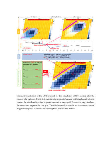
Schematic illustration of the GMR method for the calculation of SST cooling after the passage of a typhoon. The first step defines the region influenced by the typhoon track and records the initial and terminal impact times for the target grid. The second step calculates the maximum response for this grid. The third step calculates the maximum response of all grids composed to the last SST cooling field by the GMR method.
Figure 3.
Schematic illustration of the GMR method for the calculation of SST cooling after the passage of a typhoon. The first step defines the region influenced by the typhoon track and records the initial and terminal impact times for the target grid. The second step calculates the maximum response for this grid. The third step calculates the maximum response of all grids composed to the last SST cooling field by the GMR method.

Figure 4.
(a–c) SST response field during the passage of Typhoon Megi (2016) evaluated by the ADR, DMR and GMR methods. (d) Evolution of the SST at three different points corresponding to P1, P2 and P3 in parts (a–c). The fixed blue and green temporal segments represent the SST response time (from pre- to post-Megi) in the ADR and DMR methods, respectively. The red segments represent the responding and background SSTs in the GMR method.

Figure 5.
Results calculated by the ADR, DMR and GMR methods for 2004–2018: (a) average typhoon-induced SST cooling; (b) average typhoon-induced area of strong SST cooling; (c) average typhoon-induced area of 3 °C SST cooling; and (d) average typhoon-induced heat flux anomalies.
Figure 5.
Results calculated by the ADR, DMR and GMR methods for 2004–2018: (a) average typhoon-induced SST cooling; (b) average typhoon-induced area of strong SST cooling; (c) average typhoon-induced area of 3 °C SST cooling; and (d) average typhoon-induced heat flux anomalies.

Figure 6.
(a,b) The background and responding dates calculated by GMR method. (c) The SST cooling difference between DMR and GMR methods. (d) The SST change (recovery) from the grid-based maximum responding time to 24 October.
Figure 6.
(a,b) The background and responding dates calculated by GMR method. (c) The SST cooling difference between DMR and GMR methods. (d) The SST change (recovery) from the grid-based maximum responding time to 24 October.

Figure 7.
Sensitivity analysis. (a,b) Result calculated over five days with a radius of 400 km, changing the background SST two-day average pre-typhoon to a one-day and three-day average. (c,d) Results based on the background SST calculated as a two-day average SST pre-typhoon for five days after the typhoon, changing the radius from 400 to 300 and 500 km. (e,f) Results based the background SST calculated as a two-day average SST pre-typhoon for a radius of 400 km, changing five days to four and six days.

© 2020 by the authors. Licensee MDPI, Basel, Switzerland. This article is an open access article distributed under the terms and conditions of the Creative Commons Attribution (CC BY) license (http://creativecommons.org/licenses/by/4.0/).
Share and Cite
MDPI and ACS Style
Li, J.; Sun, L.; Yang, Y.; Cheng, H. Accurate Evaluation of Sea Surface Temperature Cooling Induced by Typhoons Based on Satellite Remote Sensing Observations. Water 2020, 12, 1413. https://doi.org/10.3390/w12051413
AMA Style
Li J, Sun L, Yang Y, Cheng H. Accurate Evaluation of Sea Surface Temperature Cooling Induced by Typhoons Based on Satellite Remote Sensing Observations. Water. 2020; 12(5):1413. https://doi.org/10.3390/w12051413
Chicago/Turabian StyleLi, Jiagen, Liang Sun, Yuanjian Yang, and Hao Cheng. 2020. "Accurate Evaluation of Sea Surface Temperature Cooling Induced by Typhoons Based on Satellite Remote Sensing Observations" Water 12, no. 5: 1413. https://doi.org/10.3390/w12051413
Note that from the first issue of 2016, this journal uses article numbers instead of page numbers. See further details here.