CFD Modelling of Particle-Driven Gravity Currents in Reservoirs


1
Christian Doppler Laboratory for Sediment Research and Management, University of Natural Resources and Life Sciences Vienna, Muthgasse 107, 1190 Vienna, Austria
2
Institute of Hydraulic Engineering and River Research, Department of Water–Atmosphere–Environment, University of Natural Resources and Life Sciences Vienna, Muthgasse 107, 1190 Vienna, Austria
*
Author to whom correspondence should be addressed.
Water 2020, 12(5), 1403; https://doi.org/10.3390/w12051403
Submission received: 20 April 2020
/
Revised: 9 May 2020
/
Accepted: 10 May 2020
/
Published: 15 May 2020
(This article belongs to the Special Issue Advanced Modelling Strategies for Hydraulic Engineering and River Research)
Abstract
:Reservoir sedimentation results in ongoing loss of storage capacity all around the world. Thus, effective sediment management in reservoirs is becoming an increasingly important task requiring detailed process understanding. Computational fluid dynamics modelling can provide an efficient means to study relevant processes. An existing in-house hydrodynamic code has been extended to model particle-driven gravity currents. This has been realised through a buoyancy term which was added as a source term to the momentum equation. The model was successfully verified and validated using literature data of lock exchange experiments. In addition, the capability of the model to optimize venting of turbidity currents as an efficient sediment management strategy for reservoirs was tested. The results show that the concentration field during venting agrees well with observations from laboratory experiments documented in literature. The relevance of particle-driven gravity currents for the flow field in reservoirs is shown by comparing results of simulations with and without buoyant forces included into the model. The accuracy of the model in the area of the bottom outlet can possibly be improved through the implementation of a non-upwind scheme for the advection of velocity.
1. Introduction
Reservoir sedimentation is an increasingly important challenge that operators worldwide are facing [1,2,3,4]. Storage capacity lost results in a decrease of energy production [5]. Moreover the interruption of sediment continuity impacts the downstream river morphology causing ecological problems. Thus efficient sediment management is important for economical, technical and environmental reasons [1,6].
Turbidity currents are the main transport mechanisms for fine sediments in reservoirs. They can even redistribute the material inside the reservoir [7]. In literature turbidity currents are also referred to as particle-driven gravity currents. They represent a group of density currents in which density differences result from the spatial distribution of concentration of a particulate substance. In contrast to other density currents where density differences are caused by e.g., concentration variations of a diluted substance or by temperature variations there occurs a relative velocity between the dispersed phase and the ambient phase [8]. This relative velocity is a result of gravitational (settling) and inertia forces [9].
Field observations of turbidity currents are difficult to accomplish due to their rare occurrence, for example during floods [9,10]. In addition turbidity currents usually form on the bottom of large and deep reservoirs [7] which are difficult to reach. Thus the analysis of such currents in real reservoirs is often limited to time series of point measurements of flow properties at different locations. Some studies focus on the analysis of the consequences of turbidity currents such as bottom elevation changes [7,11]. The use of satellite imaginary for turbidity measurements over larger areas (e.g., [12]) is not considered applicable for the study of turbidity currents, because this method provides turbidity data only for the near surface region of the reservoir. In addition, in most cases the spatial resolution of the available images will not be high enough.
Physical laboratory experiments have been undertaken to enhance process understanding of density currents in general (e.g., [13,14,15,16]) and also particle-driven gravity currents in particular (e.g., [17,18,19,20,21,22,23]). Lock exchange experiments are a common approach of studying gravity currents. They feature a certain volume of sediment laden fluid which is released into still ambient fluid by removing a lock which is initially separating two compartments [13,15,16,18,19,20]. The main parameter studied in these experiments is the flow front advance of the gravity current with time. In addition, the current height and sediment deposition are often recorded.
Huppert and Simpson [13] discuss several theoretical concepts describing gravity currents and study their efficiency in the laboratory on lock exchange experiments. They categorize the temporal development of the turbidity current into three regimes: (i) Right after the release of the suspension the gravity current passes through the slumping phase, in which the buoyant force is in balance with the counterflow of the ambient fluid; (ii) After this initial phase, in which the velocity is fairly constant, the gravity current is in the inertia-buoyancy phase in which it is balanced by forces of inertia; (iii) The final stage of a gravity current is the viscous-buoyancy regime where it is balanced by viscous forces [13].
Experiments with constant inflow and sediment supply have been carried out (amongst others) by Baas et al. [21] and Sequeiros et al. [22,23]. The former studied the expansion of high-concentration turbidity currents on a horizontal plate and the following deposition of sediments on that plate [21]. The latter carried out experiments with constant inflow and sediment supply studying self acceleration of turbidity currents due to sediment uptake [22].
Venting of turbidity currents has the potential of enabling highly efficient sediment management in reservoirs, satisfying economical as well as ecological needs [3,10,17,24]. The aim of this sediment management strategy is to route turbid water through bottom outlets as soon as it reaches the dam [3]. Water losses through venting are generally lower than the amount of water lost by flushing. In addition, sediment continuity can be maintained to a high degree [3,24]. As for any sediment management strategy for reservoirs, a detailed process understanding of the driving sediment transport processes is particularly crucial for efficient venting of turbidity currents [1,24].
Laboratory studies investigating particularly the formation and evolution of turbidity currents in a reservoir during venting have been performed by Fan and Chamoun et al., The former gathered general knowledge on turbidity currents and their development during venting [17]. The latter elaborated optimum conditions for venting in terms of bed slope of the reservoir [25], venting degree [24] and timing of venting [26]. With the advance of computational fluid dynamics (CFD), the experimental set-up of lock exchange experiments has been taken up for numerical studies [8,9,14,27,28,29,30,31]. Flow in these models is purely driven by gradients in the spatial distribution of density. Thus they provide an efficient test case for the validation of solvers for models of density currents. In models particularly for the simulation of fluid flow in reservoirs the set-up of lock exchange experiments imitates the inflow of turbid water during a short term storm event.
Sediment transport in these models is implemented in different detail. One-way coupling of momentum exchange between the ambient and the dispersed phase can be achieved using advection-diffusion equations [8,29,32]. In these models the particle velocity equals the sum of the fluid velocity and the fall velocity. Hence forces of inertia are neglected [8,29]. In addition, the dispersed phase is neglected in the mass conservation equation. Buoyant forces are accounted for through a source term in the momentum equation and neglected for all other terms rather than gravitational terms (Boussinesq approximation) [8,29,33]. This limits the applicability of such models to small mass loadings [8,29].
An et al. [29] simulated different kinds of gravity currents including particle driven gravity currents produced by lock exchange experiments from Gladstone et al. [19]. The focus of this study was on the differences in large eddy simulations and Reynolds averaged simulations of gravity currents. Similarly, Stancanelli et al. [30] studied the differences of LES and RANS numerically but using the setup of Musumeci et al. [15] and Stancanelli et al. [16], where the high density fluid was released into an oscillating ambient fluid [30]. Both models ([29,30]) were solved using the commercial FLOW-3D CFD code.
On the basis of their results An et al. [29] classify particle-driven gravity currents into three regimes with respect to the deposition rate of the sediment. When particles are small (e.g., < 16 µm) and hence fall velocity is low deposition has only little influence on the propagation of the gravity current (suspended regime). When suspended particles are larger (e.g., 16 µm < < 40 µm), the propagation of the gravity current is highly influenced by the fall velocity (mixed regime). Particle-driven gravity currents with larger particles (e.g., > 40 µm) rapidly loose momentum due to deposition (deposition regime). Exemplary particle sizes mentioned above apply to particles with a relative density of = 3.22. [29].
Necker et al. [8] studied the development of a particle-driven gravity current in several further aspects. The numerical data is compared to experimental data of DeRooij and Dalziel [20]. Additional data is retrieved from a high resolution numerical model as well as laboratory experiments carried out by Bonnecaze et al. [18]. Main points studied by Necker et al. were (i) the structure of the flow front, (ii) conversion of potential energy to kinematic energy and (iii) dissipation of energy due to particle settling. In addition the difference between 2D and 3D models of turbidity currents is discussed. Resuspension of particles is considered to the point that the authors show using Shields critical velocities [34] that resuspension is unlikely to occur in the studied flows [8].
Two-way coupling is necessary for higher mass loads and to account for inertial effects [9,31,35]. A model treating water and sediment as separate continua has been set up using the commercial code FLUENT by Georgoulas et al. [9]. With this model they reproduced the lock exchange experiments of Gladstone et al. [19] and simulated the expansion of high concentration turbidity currents on a horizontal plane as physically investigated by Baas et al. [21]. Cantero et al. [31,35] accounted for inertial effects using an Eulerian equilibrium approach. They carried out a direct numerical simulation of turbidity currents on a 2D Eulerian-Eulerian model.
A simplified approach for modelling the two-phase flow of a water-sediment suspension including buoyant forces has been proposed by LaRocca et al. [14,27] using the two-layer shallow water equations. Their approach is based on the assumption that the upper layer of lighter fluid remains flat during the motion. In addition to the commercial codes mentioned above, also the freeware Delft3D-FLOW model [33] developed by Deltares provides the capability of modelling particle-driven gravity currents for river applications.
Despite this large number of studies on investigating the basic process of the formation and development of turbidity currents in test cases physically and numerically, only a reduced number of works on turbidity currents in operational reservoirs has been found in literature. Exemplary, simulations of turbidity currents in reservoirs during flood events have been carried out for the Luzzone Lake, Switzerland [7], the Lugano Lake, Switzerland/Italy [36] and the Imha Reservoir, South Korea [32]. The former two models were solved using the CFX-4 code, while the latter was solved with the FLOW-3D model presented in an earlier study by the same authors [29].
Hillebrand et al. [37] simulated the flow field and sediment transport including bottom elevation changes in the Iffezheim hydropower reservoir. They used the freeware SSIIM developed at the Norwegian University of Science and Technology (NTNU) [38] for their model. This code accounts for the effects of density changes on turbulence but not for buoyant forces [39].
A two-dimensional simulation of turbidity currents in the Shimen Reservoir, Taiwan, has been carried out by Huang et al. [10], using the 2D layer-averaged turbidity current model SRH2D [40]. The method used to model turbidity currents in this model is similar to what has been proposed by LaRocca et al. [14,27]. For the study of venting Huang et al. applied a two stage approach using the empirical Rouse equation [41] for the estimation of the sediment released through the outlets at the dam.
The model set up by Lee et al. [11] simulating turbidity currents in Tsengwen Reservoir in Taiwan during typhoon-induced food events is the only model found in literature in which venting is included. The model based on the CFX-12.0 code was validated against a laboratory experiment with a setup similar to the experiments carried out by Chamoun et al. [24,25,26]. Additionally, the model of the real reservoir was validated using concentration measurements at different elevations near the dam. Based on their results, Lee et al., developed a formula for the estimation of the concentration of the vented suspension [11].
Apart from the study by Lee et al. [11] no other 3D model applications particularly studying venting of turbidity currents have been found in literature. On the one hand, such a numerical tool can provide the basis for the design of an efficient venting system for reservoirs Lee et al., Numerical models are more flexible for geometry adaptions than physical models. They are free of scaling errors and allow an analysis of the entire flow field in high detail. They can be used to study the development of a turbidity current at the actual site of a reservoir which is usually difficult to rebuild in every detail in a laboratory. On the other hand, Lee et al. pointed out that the required fine discretization and thus long computation times make it impractical to run such a model on a normal desktop computer in real time [11].
Hence this study aims to develop a numerical model allowing to study turbidity currents in real reservoirs. The basic hydrodynamic model used is RSim-3D [42,43,44]. This model is adopted for the simulation of turbidity currents through a source term in the momentum equations. Basic model verification and validation is carried out reproducing the lock exchange experiments by Gladstone et al. [19]. Moreover, results of the experiments by Chamoun et al. [24,25,26] were used for further optimization of the tool to study the development of turbidity currents in reservoirs. Thus, in a second step, these experiments are reproduced with the developed model.
2. Materials and Methods
2.1. Governing Equations and Model Setup
2.1.1. Hydrodynamic Model
RSim-3D is a computational fluid dynamics code solving the incompressible three-dimensional Navier-Stokes equations on a polyhedral mesh [42,45]. The equations are Reynolds averaged optionally using the standard k- [42] or the k- [46] turbulence model.
in Equation (1) represents the conservative property which is transported through the domain. It is replaced with the velocity for the momentum equation in the respective direction or 1 for the continuity equation. Similarly the diffusion coefficient is dependent on the particular conservative property. For the momentum equations, the diffusion coefficient is calculated as where represents the dynamic viscosity of the fluid and the turbulent viscosity. The turbulent viscosity is estimated based on the standard k- turbulence model [47]. is the fluid density. Sources and sinks are added in the source term . For the momentum equations the source term includes the pressure gradient . For the mass conservation equations is generally 0 with the exception of Dirichlet boundaries [42].
2.1.2. Sediment Transport Model
Suspended sediment transport is modelled using an advection-diffusion equation which is of the same generic form as the Navier-Stokes Equations (1). This approach has already been used for similar models in literature (e.g., [29,38]). The conservative property is the volumetric sediment concentration c. Sediment diffusivity is calculated as the quotient of turbulent viscosity and the Schmidt number.
Sediment settling is implemented through the source term by adding the term , where is the fall velocity of the particles. A set of different equations for the estimation of the fall velocity of particles with a diameter has been added to the code. The implemented approaches include the formula by Atkinson et al. in which the fall velocity in m s−1 equals the particle diameter in m to the power of 1.3 [48]. In addition Stokes fall velocity [49] has been added to the code in a three-dimensional form. The equation is piecewise continuous and has discontinuities at = 100 µm and = 1000 µm.
is the acceleration due to gravity, particle density (dispersed phase) and the density of the particle fluid suspension. The latter is calculated as the volume average of the fluid density and the particle density [19,24].
Tritthart et al. [50] analysed different approaches [48,49,51] for estimating settling velocity. They found that their results differ up to three orders of magnitude. In consequence the selection of the approach for estimating fall velocity should be the outcome of a calibration process. For the experiments reproduced in the validation of the code in this study best results have been achieved using the Stokes fall velocity [49] in Equation (2).
When sediment particles reach the bottom cell, they can settle “through” the bottom boundary and this way leave the domain. In preliminary tests this approach has proven to be most efficient for the cases studied in this article. Other approaches like applying a reference sediment concentration [49] based on bottom shear stress [34] or accumulating sediment in the bottom cell are mesh dependent. For later analysis of the amount of sediment deposited, the volume of sediment that has settled through the bottom cell is recorded.
Resuspension of sediment is not included in the implementation of bottom exchange used in this study. However it is not expected that the process plays an important role in the investigated cases as the laboratory channels did not have a loose bed [19,24]. Particles accumulating on the bottom through settling are neglected. In addition flow velocities are generally low in the test cases in this study [8]. Nevertheless resuspension might become relevant when applying the model to real reservoirs with loose beds [22,23].
2.1.3. Buoyant Forces
2.1.4. Discretization
The Navier-Stokes Equation (1) including the advection-diffusion equation as well as the source terms described above are discretized on a polyhydral mesh applying the finite volume method. The dominant cell shape of the horizontal descretization is hexahedral, while the vertical mesh is structured [42,43]. A plan view on a mesh for the numerical solution of the experiments from Gladstone et al. [19] is displayed in Figure 1.
2.2. Code Validation and Mesh Sensitivity Analysis
Code validation was carried out with particular focus on its capability of modelling turbidity currents. This capability has been here newly implemented into the RSim-3D code. The hydrodynamic model of RSim-3D has already been validated in various test cases (e.g., [42,43,52]) as well as real river applications (e.g., [52,53]). In addition the suspended sediment transport model has been used for several earlier studies (e.g., [44,54,55,56,57])
The code was validated against results of a set of lock exchange experiments published by Gladstone et al. [19]. The experiments feature a 5.7 m long and 0.2 m wide channel with horizontal bed and constant water level of 0.4 m. On one end of the channel a 0.2 m long section is initially separated by a lock and filled with water-sediment suspension instead of clear water (see Figure 1). The volumetric concentration of the suspension amounts to 3490 ppm. Amongst other data, time series of flow front advance distances after removal of the lock are provided for several different experimental runs. The experiments differ in the grain size of the sediment. The density of the sediment used by Gladstone et al. was 3217 kg m−3 [19]. Sediment density, volumetric sediment concentration and channel width as characteristic length scale correspond to a Grashof number of about 1.9 × 10⁸.
The following four experiments carried out by Gladstone et al. [19] have been reproduced numerically using the RSim-3D code with the newly implemented source term accounting for buoyant forces:
- Case A: one grain fraction with = 25 µm and = 0.8 mm s−1.
- Case D: two grain fractions to equal amounts with = 25 µm and = 69 µm and = 0.8 mm s−1 and = 5.8 mm s−1, respectively.
- Case G: one grain fraction with = 69 µm and = 5.8 mm s−1.
- Case R: five grain fractions to equal amounts with = 17 µm, = 37 µm, = 63 µm, = 88 µm and = 105 µm and = 0.3 mm s−1, = 1.7 mm s−1, = 4.8 mm s−1, = 9.4 mm s−1 and = 11.3 mm s−1, respectively.
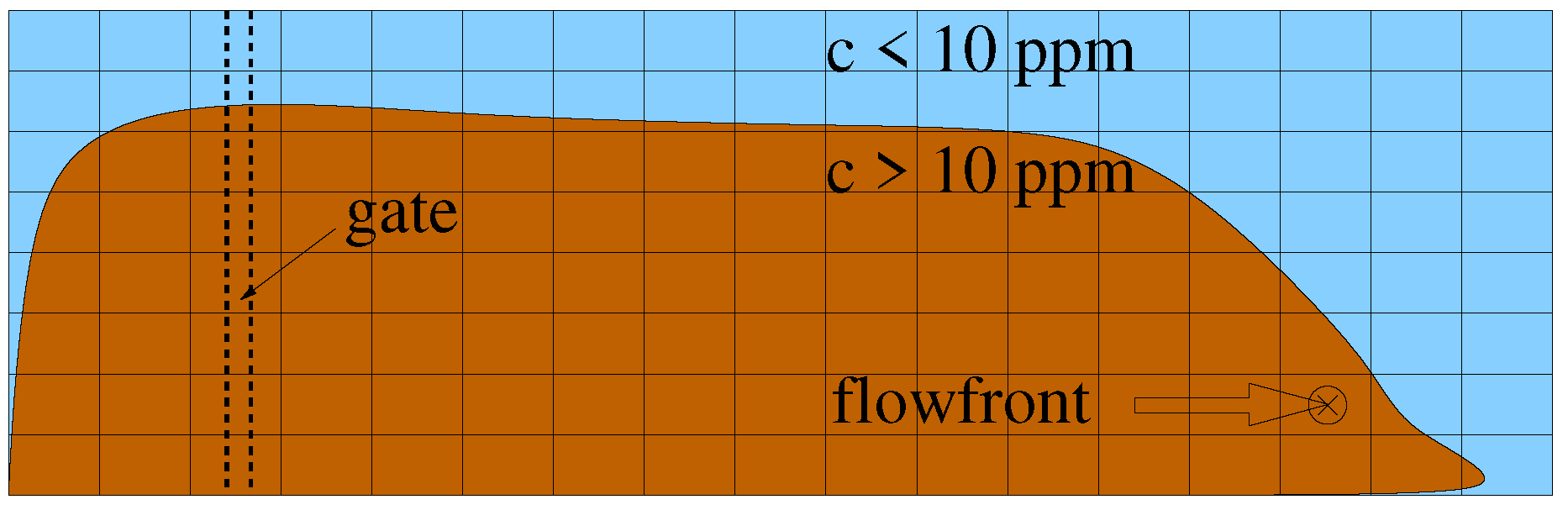
Flow front advance in the lock exchange experiments was monitored by Gladstone et al., by measuring the distance between the flow front and the gate in regular intervals of 3 s [19]. In the numerical model the position of the flow front is defined at the cell centre of the cell furthest from the gate in the second layer above the bottom which has a sediment concentration higher than 10 ppm (see Figure 2).
To study the discretization error and test mesh convergence the model was run on four different meshes using five different time steps. Table 1 displays the cell sizes and time steps with approximate maximum Courant numbers which were used in the numerical model of the lock exchange experiments [19].
The following boundary conditions were applied in the model: no-slip boundary condition for the bottom and side walls, a symmetry boundary condition for the free surface and a zero gradient velocity boundary condition with fixed pressure at the outlet. Although there was no inflow velocity in the physical experiments [19], an inflow velocity of 1.25 × 10⁻⁵ m s−1 (0.001 L s−1) was applied at the inlet for stability reasons.
2.3. Test Case for the Study of Turbidity Current Venting Efficiency
The applicability of the RSim-3D-solver for the optimization of venting of turbidity currents in reservoirs was studied by reproducing the experimental set-up of Chamoun et al. [24]. In these experiments 0.001 m3 s−1 of a sediment suspension with a volumetric concentration of 2.3% (≙27 g L−1) was constantly fed into a laboratory channel. The channel representing a reservoir is initially filled with clear water so that the water depth amounts to 0.8 m. The dimensions of the channel are 6.7 m in length and 0.27 m in width. A bottom outlet 0.12 m high and 0.09 m wide is placed at the end of the channel through which water is vented at a specific flow rate [24,25,26].
Sediment properties used in the venting experiments are: = 66.5 µm, = 140 µm, = 214 µm with a density of = 1160 kg m−3 [24,25,26]. Concentration, density and channel width correspond to a Grashof number of 4.1 × 10⁸. This is of the same order of magnitude as the Grashof number in the lock exchange experiments [19] (see above). For the numerical model eight fractions of sediment size listed in Table 2 were used.
In their experiments Chamoun et al., tested the influence of the ratio of vented flow rate to the inflowing discharge (venting degree ) on venting efficiency. For this purpose the vented sediment concentration was continuously recorded. In addition sediment deposition was measured at multiple locations along the channel [24].
From the concentration and the density of the vented suspension and the vented flow rate the aspiration height according to Fan [17] is calculated [24].
When the height of the turbidity current at the dam is higher than this theoretical value, only turbid water is vented [10,17,24].
Venting efficiency was analysed with respect to global venting efficiency (GVE). Global venting efficiency is defined for a time step t as the ratio of the total sediment mass that has entered the reservoir to the vented mass of sediment until t [24].
Venting time is normalized for the sake of results comparison on the basis of the aspiration height in Equation (5) [24].
in Equation (7) is the time when venting starts ( = 150 s in all cases).
For the numerical model of venting the same types of boundary conditions were used, that were also applied in the lock exchange cases (see above). The flow rate at the inlet is set to 0.001 m3 s−1. The outlet situation including the bottom outlet for venting have been modelled in the following way: A quadratic channel with 4.4 cm edge length was attached to the end wall of the flume. This represents the venting pipe with a diameter of 5.0 cm which has the same cross sectional area. The edges between the end wall of the flume and the venting channel were rounded so that a 9 cm wide section is left open in the end wall.
Cells at the entrance to the venting channel that have cell centres higher than 12 cm above the bottom were assigned with a no-slip wall boundary condition to limit the height of the bottom outlet opening. Further downstream in the venting channel cells with cell centres less than 5 cm above the bottom are assigned with the wall boundary condition to limit the height of the venting pipe. In cases with a venting degree of < 100% the two uppermost cell layers are left open to enable overflow over the “weir”. Venting degrees of < 100% are implemented into the numerical model by assigning a fixed velocity to the “open” cells below the internal wall. The velocity in the bottom boundary cells is interpolated using a wall function [42]. Higher venting degrees of ≥ 100% are implemented through the pressure boundary condition at the outlet. The water level there is lowered with respect to the volume decrease in the channel.
After the “inlet” into the venting pipe only four cell layers in the upper third of the channel are assigned the no-slip wall boundary condition. This way the height of the venting channel is increased again to enable a stable zero-gradient outlet boundary condition.
The domain is discretized using dominantly hexahedral cells in horizontal direction and a structured mesh in vertical direction. The area of the venting pipe is meshed using dominantly quadrilateral cells. The hexahedral cells have a diameter of about 3 cm. In vertical direction 40 cell layers are used. This cell size has been found most practical in a mesh sensitivity analysis carried out by Lee et al. [11] using a similar experimental setup. Results of the mesh sensitivity analysis using the lock exchange experiments [19] in Section 4.2 show that this discretization is reasonable for the RSim3D-code as well. In total the mesh has 118,800 cells. A time step of 0.1 s is used for time discretization.
3. Results
3.1. Flow Front Advance in Lock Exchange Experiments
Figure 3 displays the development of the turbidity current in the lock exchange experiments after removal of the lock. The images show the water sediment suspension plunging below the clear water and then travelling along the bottom of the channel.
Initially the turbidity current has a triangular shape with the surface slanted towards the front of the current (Figure 3a). After the acceleration of the current, the shape of the current becomes rectangular. Its height decreases only slightly with time (Figure 3b–d).
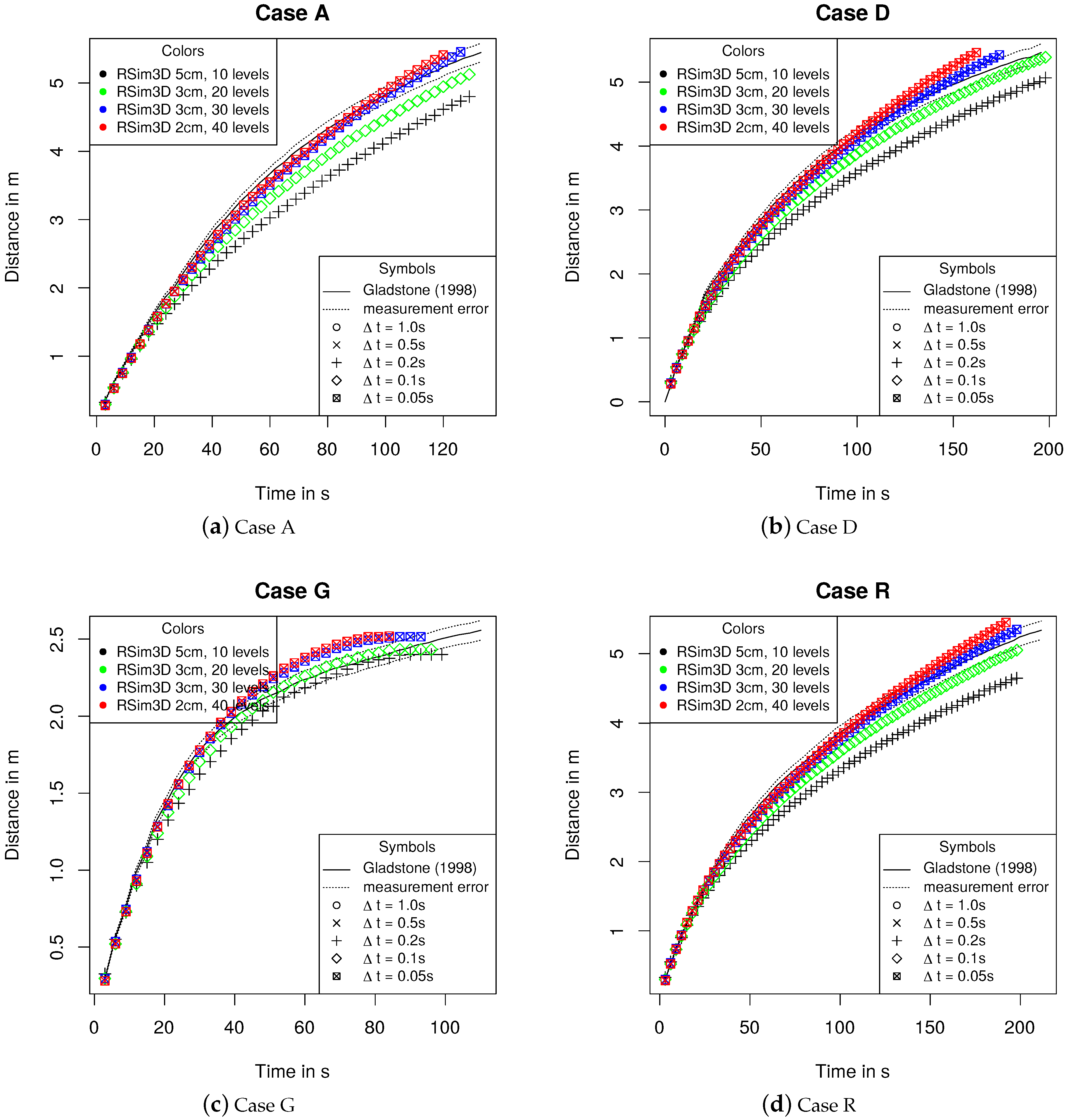
The results of the flow front advance in the numerical model are plotted against literature results [19] in Figure 4. The plots show the increasing distance between the flow front and the lock position with ongoing time after the lock removal. The initial velocity of the turbidity currents with different sediment particle size is similar in all cases. Flow front advance is decaying with time depending on the fall velocities of the particles in the respective case. In cases with small particle sizes and thus low fall velocity (e.g., case A in Figure 4a) the velocity of the turbidity current decreases only slightly. In contrast, a sharp bend is visible in the flow front advance of case G where particles are larger and thus settle faster (e.g., case G in Figure 4c).
The flow front advance in Figure 4 from the numerical simulations on coarser meshes is generally underestimated. With refinement of the mesh the results of the numerical model approach the results of the physical model. Hardly any difference is visible in results of the flow front advance from the simulations on the second finest and the finest mesh.
3.2. Computational Effort of the Numerical Models of the Lock Exchange Experiments
Table 3 displays the computation time required for Case D of the lock exchange experiments on different meshes and with different time steps. The simulations were run in parallel on an Intel i7-3770 ( 16 GB RAM) processor using four cores. Parallelization was realised using OpenMP.
The computation times in Table 3 show that the computational effort mainly increases with mesh refinement. Although the reduction of the time step requires the equations to be solved at additional time steps, computation time increases by a far lower factor than the number of time steps is increased. For some cases computation time could even be reduced by decreasing the time step.
3.3. Venting
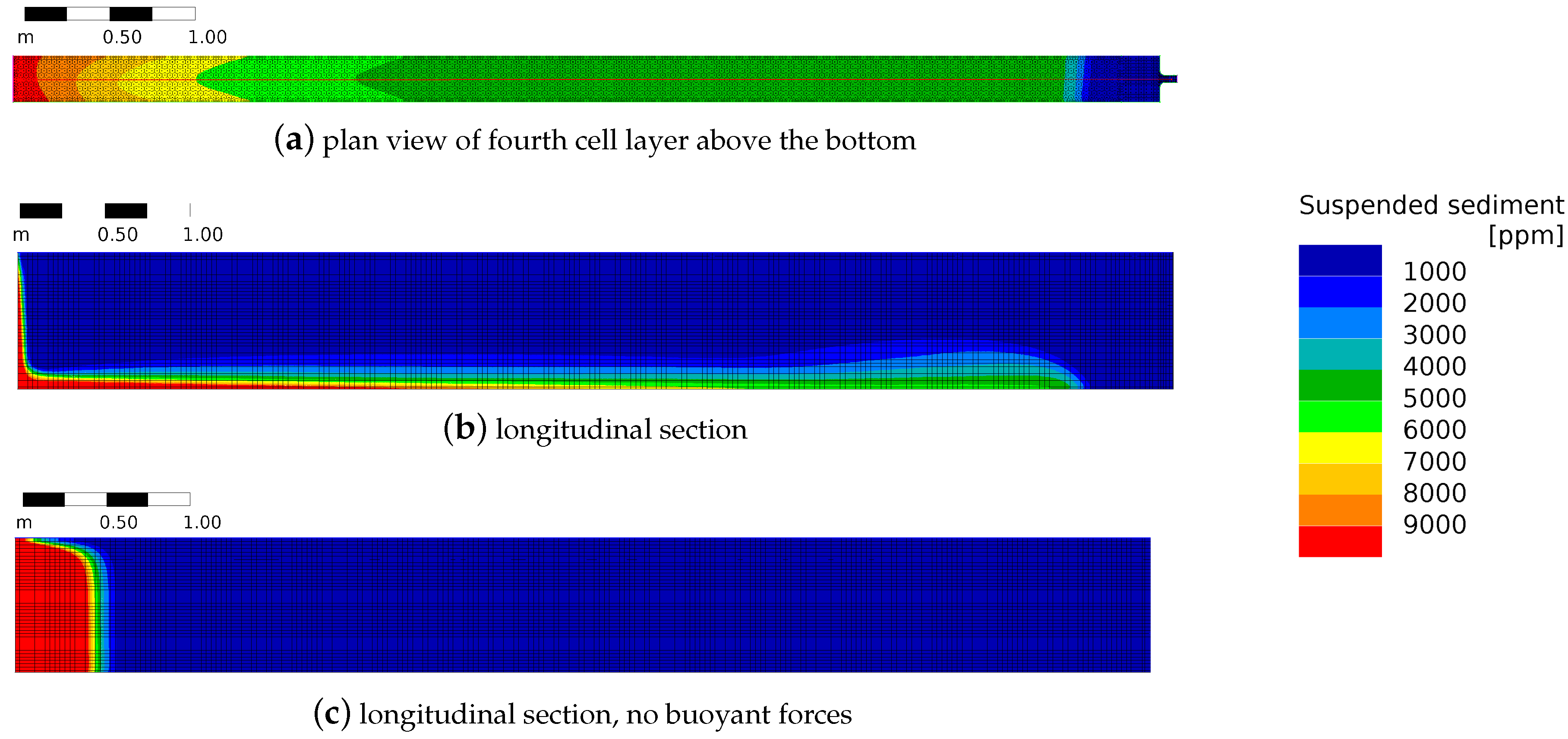
Figure 5 displays sediment contours at time = 150 s (right before the start of venting) in the numerical model of the experiments from Chamoun et al. [24]. The plan view (Figure 5a) shows the decreasing sediment concentration along the length of the turbidity current as a result of dilution and settling. The height of the current can be observed in the longitudinal section (Figure 5b). The contour plot shows the decreasing height of the turbidity current from the inlet towards the current head. At the head the current height is increasing again.
Sediment concentration decreases strongly along the first metre of the channel to approximately 25% of the inlet concentration (Figure 5a). Along the remaining part of the channel, sediment concentration is more or less constant with about 20% of the inlet concentration. The current head is apparent through the sharp drop in concentration to almost 0 ppm.
Similarly, the turbidity current height with respect to sediment concentration in the longitudinal section in Figure 5b drops mainly along the first half of a metre of the channel. From that point the slope of the surface of the current is relatively small. The minimum current height is located about 1.5 m behind the current head. From this point onwards, the current height starts to increase again.
For the purpose of comparison one extra simulation was run in which the source term for bouyant forces Equation (4) was neglected. The longitudinal section of the concentration field in the results of this simulation at = 150 s is displayed in Figure 5c. The figure shows that the sediment has been transported less than half a metre from the inlet. This transport is only driven by the velocity at the inflow boundary. The height of the current reduced slightly as a result of settling.
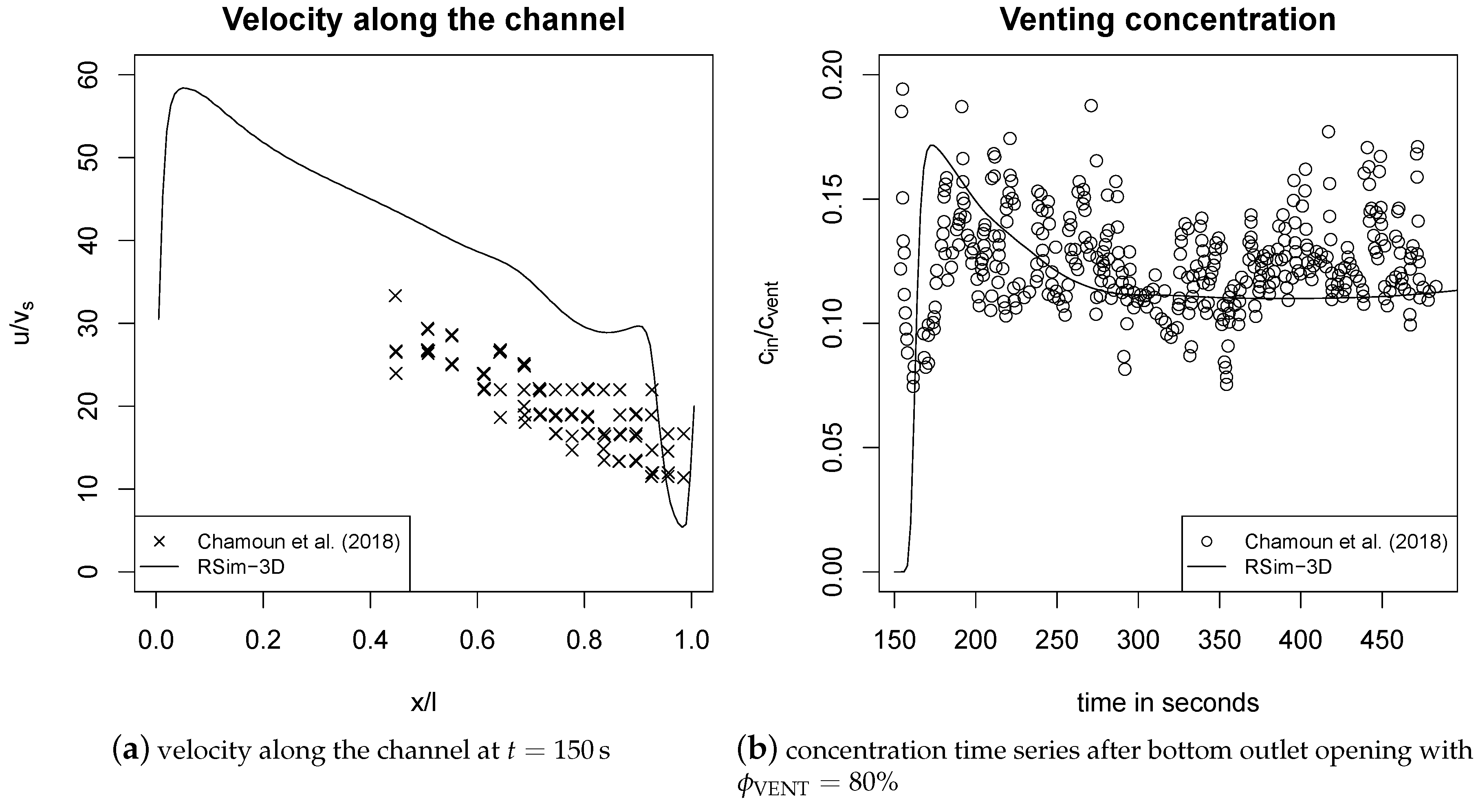
Figure 6a displays the velocity of the turbidity current along the channel length normalized with a fall velocity of 0.0015 m s−1 at time = 150 s. It can be seen that the velocity of the turbidity current decays along its length. At the beginning of the channel the velocity is almost 60 times the fall velocity. In the current head the velocity is constant with a magnitude of approximately 30 times the fall velocity. In the front of the current head the velocity drops sharply. At all points along the channel the normalized velocity of the current was slightly higher in the numerical model than in the physical model [24].
The temporal evolution of the sediment concentration of the vented suspension at a venting degree of = 80% is displayed in Figure 6b. After an initial peak vented sediment concentration of about 17% of the inlet concentration at the start of venting, the concentration approaches a constant value of about 11–12% of the inflow concentration. The concentration measured in the physical experiment [24] fluctuates around this value with an amplitude of about 5% of the inflow concentration.
Figure 7 displays a longitudinal section of the concentration field after 350 s of venting ( = 500 s). At this point the flow should have reached steady state condition [24]. The images show the reflection of the turbidity current at the end wall of the channel and the return flow caused by the reflection. The return flow is decreasing with increasing venting degree.
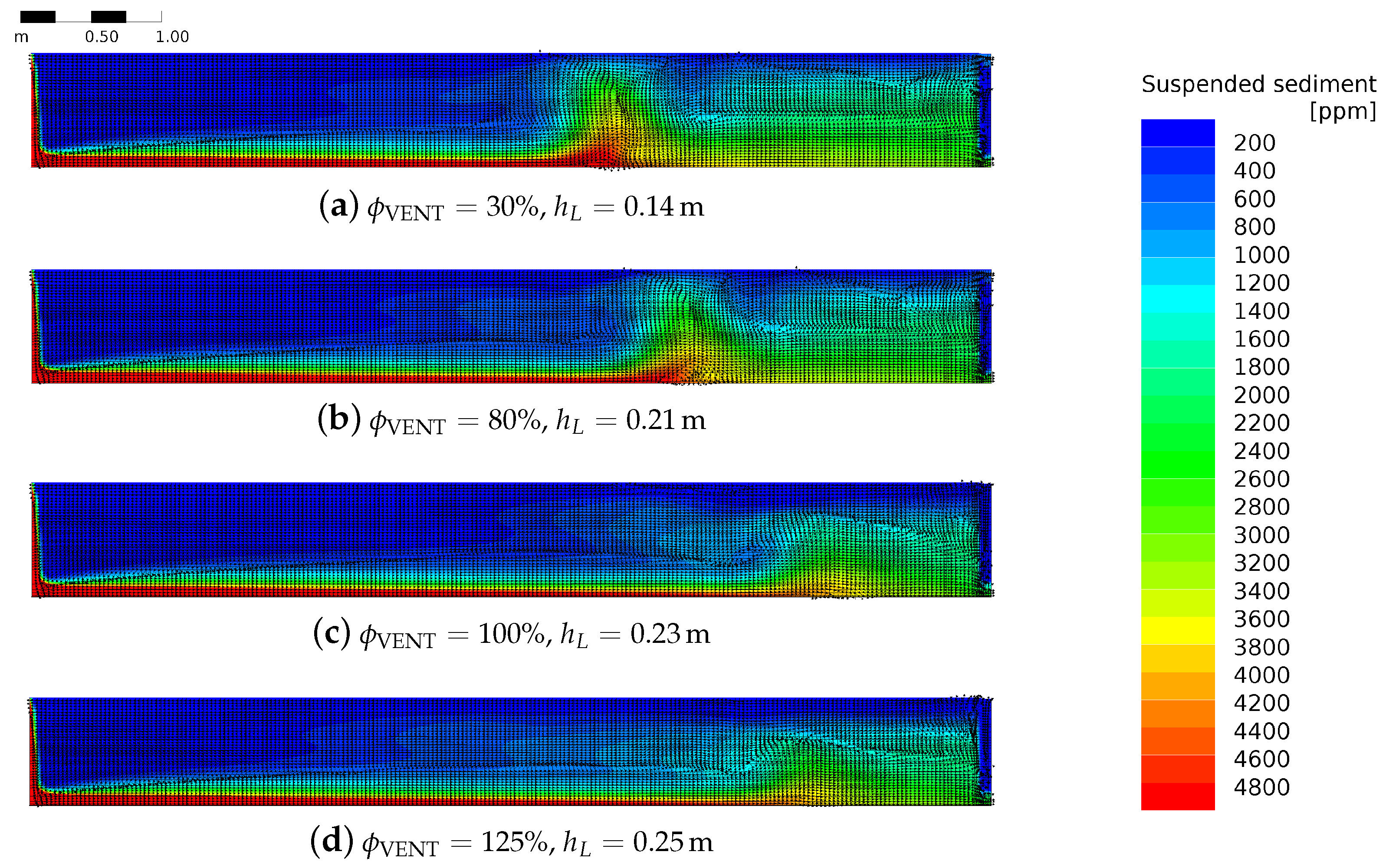
The lower the venting degree, the further the return flow travels back towards the inlet of the channel. As the return flow causes additional resistance for the arriving turbidity current, the turbidity current slows down and increases in height. This way at venting degrees of < 100% two regions with a circular flow patterns form, visible in Figure 7a,b.
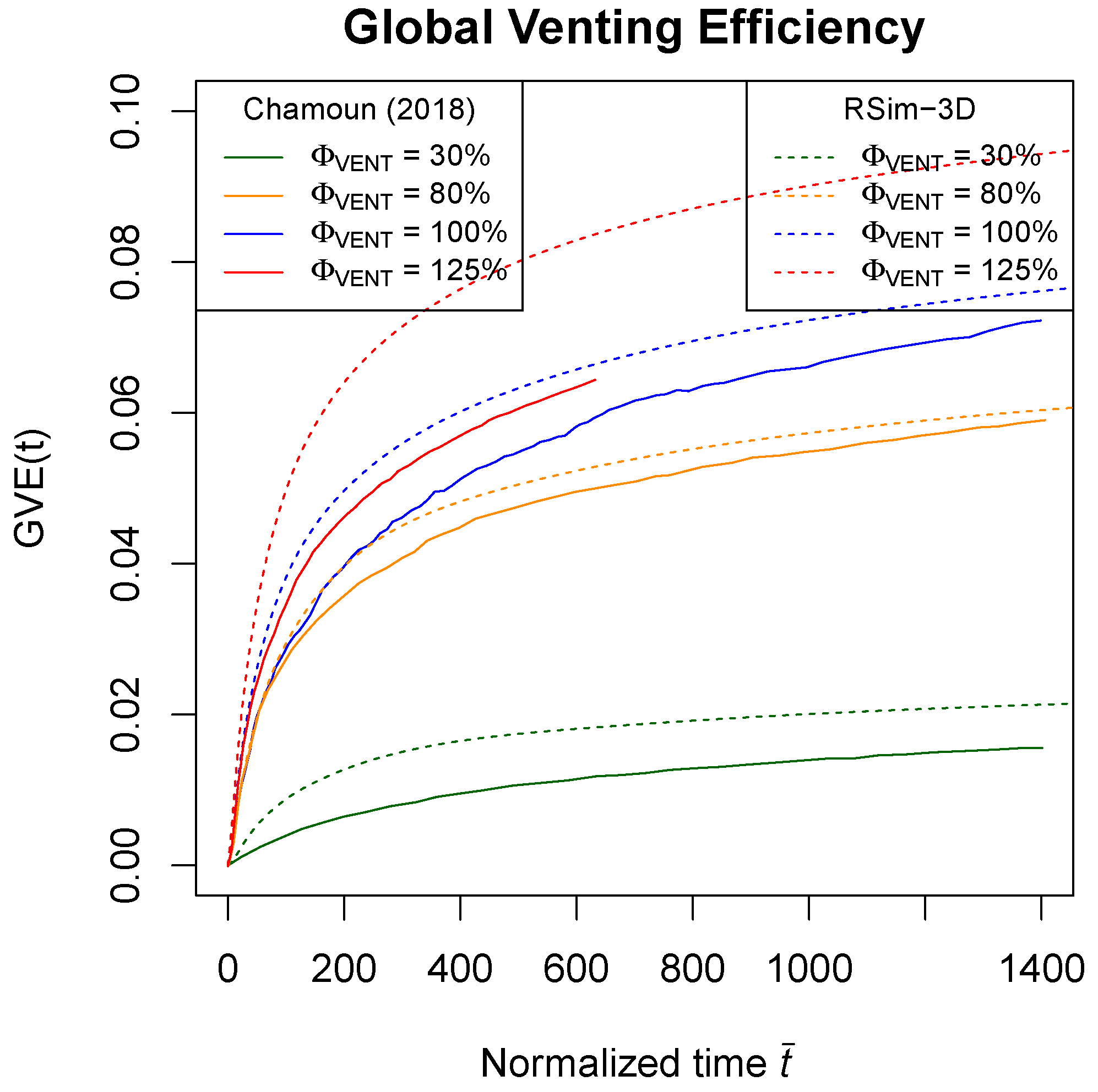
Figure 8 displays global venting efficiency and the normalized venting time . Global venting efficiency is initially strongly increasing at the start of venting. The slope of the lines is then decreasing to a constant value when the flow in the channel reaches a steady state.
The initial slope of the lines for global venting efficiency ( < 200) in Figure 8 is higher in the numerical model results than in the outcomes of the physical model. This causes a slightly higher global venting efficiency in the numerical model. After this initial period, the slope of the lines for global venting efficiency from the numerical model matches the slope of the respective lines from the physical model.
3.4. Sediment Deposition Along the Channel
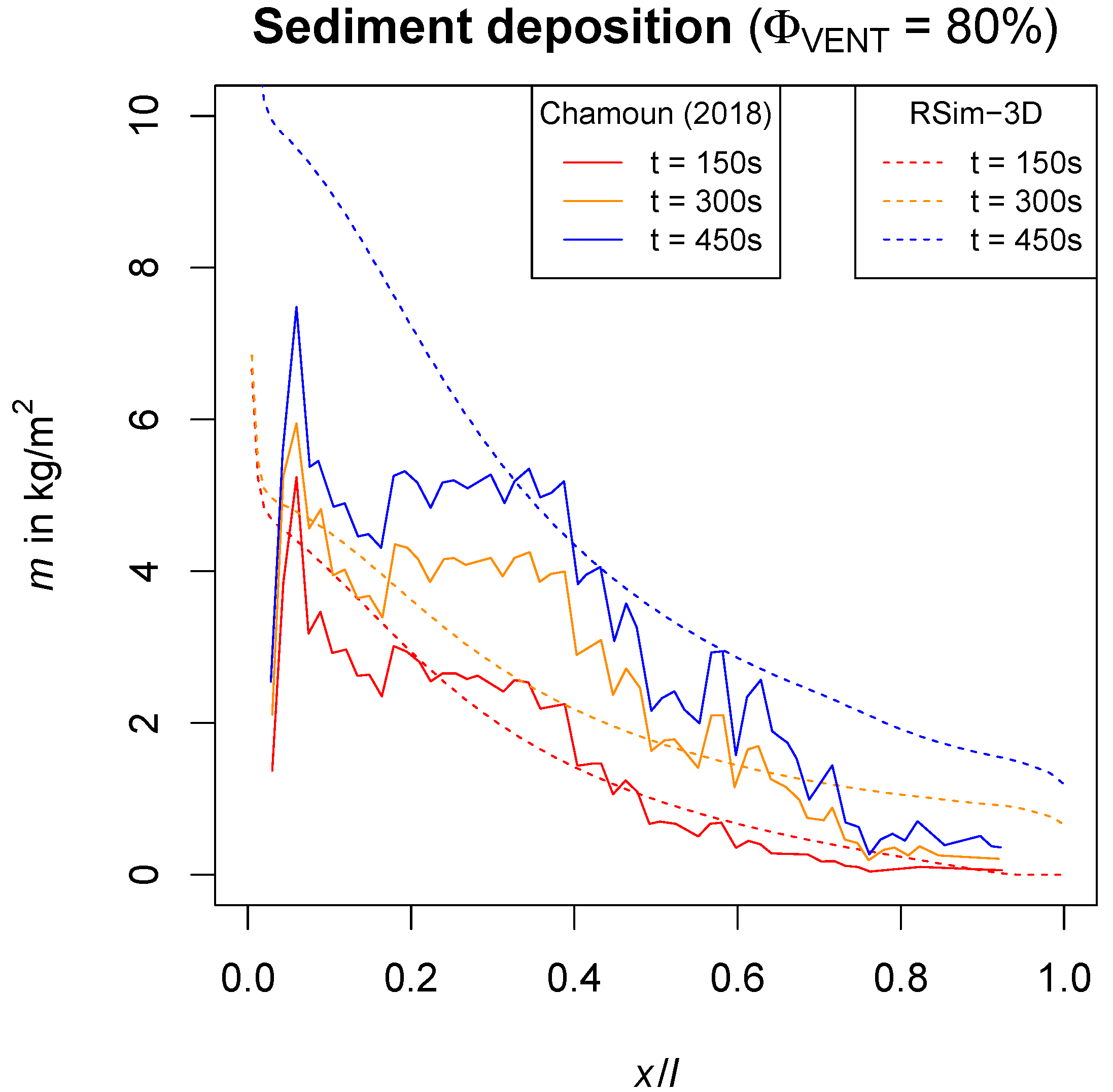
For the case with a venting degree of = 80% sediment deposition along the channel has been recorded and compared to respective measurements by Chamoun et al. [24]. The results of sediment deposition are displayed in Figure 9.
Figure 9 shows decreasing sediment deposition along the channel length. While the initial peak of sediment deposition is right at the inflow section in the numerical model results it occured slightly downstream in the physical model. For the time steps = 150 s (start of venting) the deposition in the simulation results from the RSim-3D solver agrees fairly well with the measured deposition in the laboratory experiments [24]. At = 300 s the accumulation of sediment in the second quarter of the channel visible in the physical model results is not reproduced in the numerical model, while the remaining sections are in agreement. At = 450 s sediment deposition in the numerical model is overestimated compared to the physical model along the first third of the channel length.
4. Discussion
4.1. Code Verification and Validation
The general formation of the current at different time steps during the slumping phase in Figure 3 can be compared to theoretical models and pictures from laboratory experiments (e.g., [13]). Theory in literature suggests that the total volume of the current remains constant during the slumping phase of a gravity current. In addition, the height of the current is assumed to be constant along its length so it can be approximated with rectangular boxes [13]. This theory holds true for the numerically modelled particle-driven gravity current. Particularly at time steps = 12 s and = 18 s in Figure 3c,d the surface of the turbidity current is relatively flat. Discrepancies between the results of the numerical model and the theory of gravity currents [13] can be explained by the process of particle settling. Due to this process the sediment load in the current is continuously decreasing and potential energy is lost [8].
Initial velocity of the numerically modelled particle-driven gravity current is constant and of the same magnitude for about 20 s in all cases displayed in Figure 4. This is typical for the slumping phase [13,19]. After this phase the flow front advance decays depending on the fall velocity of the particles which is described by An et al. [29].
According to the particle-driven gravity classification with respect to the deposition rate [29], the turbidity current in case A corresponds to a mixed regime. This is in contrast to case G which features a turbidity current in the deposition regime. In the latter the deceleration as a result of the setting of particles [29] can clearly be observed at 20 s < < 40 s (see Figure 4c). This shows that the code is capable of modelling the effect of particle settling described by An et al. [29].
The comparison of the flow front advance in the physical [19] and numerical model in Figure 4 allows a quantitative comparison of the results. Using sufficiently fine meshes it has been achieved to reproduce the particle-driven gravity current for all four grain size distributions considered with reasonable accuracy.
It is assumed that inaccuracies in the flow front distance towards the end of each experiment are a result of post-processing. Gladstone et al. [19] visually determined the position of the flow front which might involve inaccuracies when the turbidity becomes low as a result of dilution. In addition, when the concentration gradient at the flow front decreases the position of the flow front in the numerical model is more sensitive to the choice of the minimum concentration defining the flow front (10 ppm, see Section 3.1).
4.2. Mesh Sensitivity Analysis and Quantitative Error Analysis
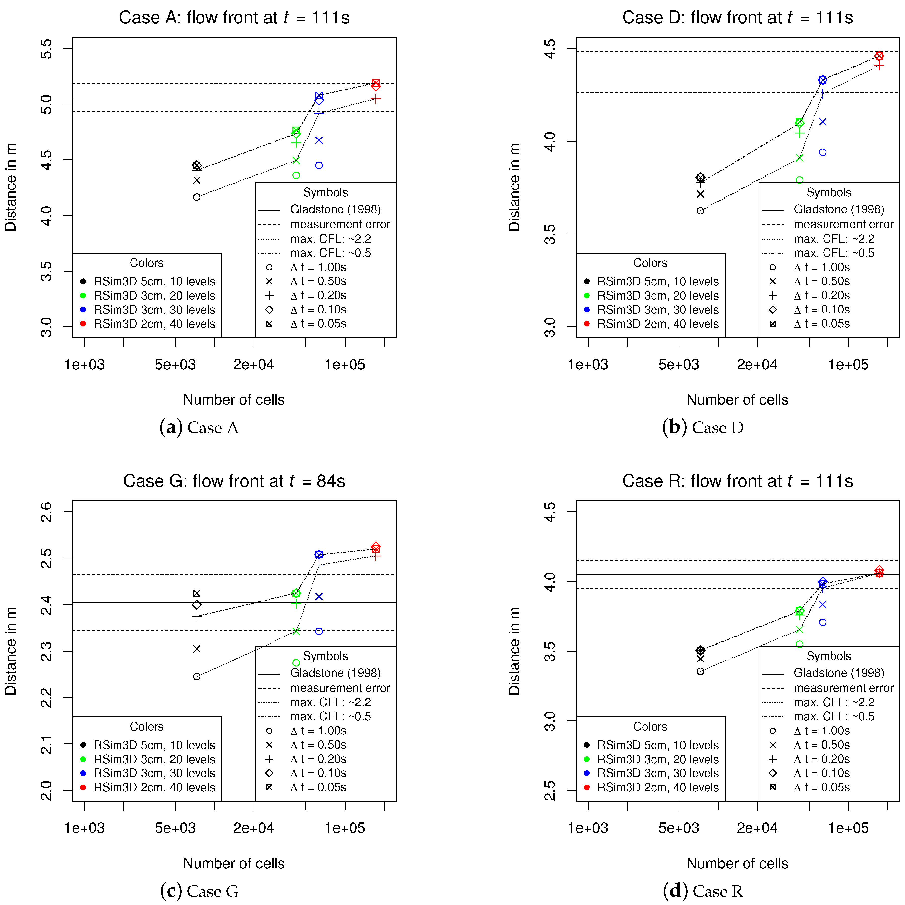
To study mesh convergence Figure 10 displays the position of the flow front at time = 111 s for cases A, D and R and = 84 s for case G, respectively. The displayed results have been retrieved from simulations on different meshes and with different time steps. In all cases the curve flattens with increasing mesh refinement, showing mesh convergence. The curves have the steepest slope between the results of the meshes 3vl20 (42,160 cells) and 3vl30 (63,240 cells). Between those two meshes a refinement is only made in the vertical direction. This suggests that sufficient fine vertical spatial discretization is particularly crucial for modelling turbidity currents. Further discussion of the mesh convergence on the basis of the grid convergence index [58,59] has been dismissed. The complexity of the mesh and different refinement ratios in horizontal and vertical direction make this approach impractical.
For cases A, D and R the flow front advance in Figure 10 approaches a value within the boundaries of accuracy of the measured flow front advance from the physical model [19]. In case G flow front advance in the numerical model is higher than the measured flow front advance. This suggests that the fall velocity estimated using Equation (2) might be too low. In such cases the accuracy can possibly be optimized for the particular particles in the suspension by calibration with respect to fall velocity (see also Section 2.1.2).
Table 4 displays normalized Euclidean norms (-norms, Equation (8)) of the error (difference) between the flow front advance in the numerical and the physical model. To compare the error norms of simulations with different numbers of saved time steps, the norms are normalized by division by the number of data points n.
For all cases -norms in Table 4 remain relatively constant or are even slightly increasing with refinement from the second finest to the finest mesh. Similarly, the reduction of the time step from the second lowest to the lowest did only result in minor changes of the error norms. This suggests that the discretization error has been reduced to a minimum. The remaining error is driven by other factors rather than spatial or temporal discretization. These include model assumptions such as the estimation of fall velocity using Equation (2) or simplifications (see Section 2.1). Thus mesh convergence has been achieved.
For cases A, D and R -norms are decreasing with the first three steps of mesh refinement. While a decrease of the error has been achieved with further mesh refinement to the finest mesh in case A, error norms are slightly increasing on the finest mesh in the other cases.
In contrast -norms in case G are increasing with refinement of the mesh 3vl20. This can be explained with the overestimation of the flow front advance in this model (see above and Figure 4c, Figure 10c). Despite this, the -norm is approaching a constant value on the fine meshes which shows that mesh convergence has been achieved (see above).
In conclusion, a horizontal cell size of 3 cm and 30 vertical layers (63,240 cells) are necessary for achieving the highest accuracy of the model of the lock exchange experiments. This agrees well with the results of the mesh sensitivity analysis of Georgoulas et al. [9]. They found an entirely structured hexahedral mesh with 68,950 cells to be most practical for a numerical model of the lock exchange experiments from Gladstone et al. [19].
In order to get best results on a certain mesh a sufficiently small time step is required. While reducing the time step substantially improves the accuracy of the results (see Figure 10 and Table 4) it comes at only minimum additional computational effort (see Table 3). The low increase in computation time compared to the additional number of time steps for which the equations need to be solved can be explained by the smaller number of iterations required for the SIMPLE solver to converge at each time step.
4.3. Venting
The shape of the turbidity current in Figure 5 matches the data from the physical experiments [24]. The height of the current in the results of the numerical model is about 40% of the channel height. This is 10% less than the current height observed by Chamoun et al. [24]. The reason for this underestimation can possibly be insufficient accuracy of the Stokes fall velocity Equation (2). In addition, the approximation of the grain size distribution in Table 2 might be inaccurate since only values for , and are provided by Chamoun et al. [24]. The return flow caused by the reflection of the turbidity current at the end wall described in literature (e.g., [17,24]) is also visible in the results from the numerical model in Figure 5.
The development of convective velocity along the channel length in Figure 6a from the numerical model is similar to the measured velocity from the physical model [24]. This comes with the restriction that absolute value of normalized velocity is higher in the numerical model than the measured velocity in the physical one. As the ratio between the numerically modelled and measured velocity is more or less constant, it is assumed that this offset is caused by using only the fall velocity of the particle diameter for normalization of flow velocity. This very likely does not sufficiently represent the mixture of particles driving the turbidity current. Fall velocities of particles in the suspension range from 0.4 mm s−1 to 3.7 mm s−1 (see also Table 2). The normalized velocity in the numerical model would agree with the measured velocity in the physical model, when a fall velocity of 2.3 mm was used for normalization.
The average sediment concentration of the vented suspension is similar in the numerical and physical model [24]. The limitation in this comparison is that the temporal variation of the concentration which has been measured in the physical model has not been captured with the numerical model. It is not expected that this temporal variation causes substantial influence on the results for overall venting performance prediction. Venting performance usually is analysed integrated over time (see e.g., Equation (6)).
In the longitudinal sections of the concentration field with different venting degrees in Figure 7 return flow is clearly visible in cases with a venting degree lower than 1 (Figure 7a,b). This return flow is lower in the models with a venting degree of = 100% and = 125% in Figure 7c,d. Furthermore the figure also shows that the height of the turbidity current reduces with increasing venting degree . This matches observations described by Chamoun et al. [24].
While a clear difference in the concentration contours in Figure 7 is visible comparing the cases with = 30% (Figure 7a), = 80% (Figure 7b) and = 100% (Figure 7c) the concentration field does not appear to change with further increase of the venting degree to = 125% (Figure 7d). This agrees with the conclusion of Chamoun et al. that highest venting efficiency can be achieved with a venting degree of = 100% [24].
Comparing global venting efficiency of the numerical model with global venting efficiency of the physical model [24] in Figure 8 reveals that venting efficiency is generally overestimated in the numerical model. The overestimation of global venting efficiency in the numerical model is particularly high in the case with the highest venting degree = 125%. A possible explanation for this is the second order upwind discretization of the convection part of the Navier-Stokes momentum Equation (1) in the RSim-3D code. This scheme does not allow influence of a downstream cell on convection of velocity. Thus “suction” from the bottom outlet is only propagated to upstream cells through the pressure source term in the momentum equation and the pressure correction equation. This might cause an underestimation of the velocity in the area of the bottom outlet. As a result less clear water is vented through the bottom outlet and the concentration of the vented suspension is overestimated. To overcome this issue, a non-upwind scheme for the advection of velocity could be implemented in the model.
Sediment deposition along the channel could also be captured fairly well with the developed solver. Particularly for the earliest time step ( = 150 s) displayed in Figure 9 the deposited amount of sediment in the numerical model agrees well with the laboratory measurements [24]. In the physical model results [24] a plateau in sediment deposition occurs along the second quarter of the channel which is not captured by the numerical model. In addition, at the latest time step ( = 450 s) sediment deposition along the first third of the channel length is overestimated in the numerical model. The reason for the discrepancies between the sediment deposition in the numerical and physical model results is credited to the missing implementation of resuspension in the numerical model (see Section 2.1.2). While in reality a balance between sediment deposition and resuspension might be reached in the upstream section of the channel as soon as enough sediment has accumulated on the bottom, the latter process is not captured by the numerical model. Thus, the accumulation of sediment at the bottom is overestimated. In addition sediment might be transported from the first quarter to the second quarter of the channel as bed load. Bed load transport is also not considered in the current version of the model.
4.4. Applicability of the Code to Real Reservoirs
The results of the test cases show that the developed code can accurately model turbidity currents. Using the code it seems to be possible to numerically model the turbidity current from the entrance into the reservoir to the dam without having to rely on empirical models. This provides an advantage compared to earlier studies (e.g., [10]). In addition the solver RSim-3D has been developed with particular focus on river applications [42] while earlier studies were relying on commercial CFD codes with focus on other applications (e.g., [7,11,32,36]). This specialization of the RSim-3D solver allows to efficiently apply the developed code to real reservoirs in their natural size and shape.
The effect of density gradients as a result of different spatially distributed sediment concentrations can be seen by comparing Figure 5b,c. The development of the sediment plume is substantially different in the simulation including the source term for buoyant forces (Figure 5b) compared to Figure 5c. This observation agrees with the statement of DeCesare et al. that turbidity currents are the main transport mechanism for sediments in reservoirs [7]. In consequence it can be concluded that buoyant forces should be a substantial part of computational fluid dynamics models of reservoirs.
Limitations in the current version of the model are related to the storage type of the reservoir. Water in reservoirs for long term storage often has a different temperature than the inflowing water. Thus density differences also result from temperature gradients which are neglected in the current version of the model. Hence the application of the RSim-3D solver for turbidity currents is limited to reservoirs for short term storage.
The mesh sensitivity study shows that reasonable results can be achieved even on rather coarse meshes. The computation time on a desktop computer of the model of the lock exchange cases was less than half an hour using the coarsest mesh (5vl12, 7280 cells) and between two and three days (depending on the convergence) using the finest mesh (2vl40, 172,200 cells, see Table 3). This is particularly relevant considering the problem of long computation times with 3D models of turbidity currents in reservoirs mentioned by Lee et al. [11]. Although the computation time is still too long for real-time studies, the model may allow a detailed analysis of the turbidity current in a reservoir in reasonable time. In order to finally confirm the applicability of the RSim-3D code to model turbidity in real reservoirs a test using a real reservoir geometry remains to be done as future work.
5. Conclusions
The existing hydrodynamic code RSim-3D [42,45] was successfully extended to model particle-driven gravity currents. Test cases show that the numerical model converges with mesh refinement and reduction of the time step. The flow front advance in lock exchange experiments agrees well with the literature data [19]. The general relevance of including gravity currents into computational fluid dynamics models of reservoirs is emphasized by comparing two simulations with and without buoyant forces. The results show that the flow in the studied test case is substantially driven by buoyant forces. Accuracy can potentially be increased through calibration of fall velocity. Further development of the model can be done by the implementation of bottom exchange including resuspension which is not mesh dependent.
Turbidity currents with continuous sediment inflow from experiments of Chamoun et al. [24] have successfully been reproduced numerically using the developed code. A comparison of the concentration field during venting shows the influence of the venting degree on the sediment distribution in the channel. A limitation of the model is the upstream propagation of the “suction” from the bottom outlet during venting. It is assumed that this is due to the second order upwind discretization scheme used for convection of velocity in the momentum equations. As a result, the vented sediment concentration at the bottom outlet is overestimated in the numerical model, particularly at higher venting degrees of > 100%. Thus to improve the accuracy of the numerical code in the immediate area of the bottom outlet a non-upwind scheme for the advection of velocity can be implemented.
Moreover, sediment deposition could be captured fairly well with the numerical model. This comes with the restriction of the missing implementation of resuspension of sediment. In addition, sediment transported as bed load in the physical model was not transported in the numerical model.
In conclusion, the test cases show that RSim-3D with the newly implemented functionality to model density currents provides the general capability to study turbidity currents in real reservoirs. The computational effort is low enough that reasonable results can be achieved on a current desktop computer in less than one week’s time.
Author Contributions
Conceptualization: D.W. and M.T.; Data curation: D.W.; Formal analysis: D.W.; Funding acquisition: M.T., C.H. and H.H.; Investigation: D.W.; Methodology: D.W. and M.T.; Project administration M.T. and C.H.; Resources: M.T. and C.H.; Software: D.W. and M.T.; Supervision: M.T. and C.H. and H.H.; Validation: D.W., M.T. and C.H.; Visualization: D.W.; Writing—original draft: D.W.; Writing—review & editing: M.T., C.H. and H.H.; All authors have read and agreed to the published version of the manuscript.
Funding
This paper was written as a contribution to the Christian Doppler Laboratory for Sediment Research and Management. In this context, the financial support by the Christian Doppler Research Association, the Austrian Federal Ministry for Digital and Economic Affairs and the National Foundation for Research, Technology and Development is gratefully acknowledged.
Acknowledgments
The computational results presented have been achieved in part using the Vienna Scientific Cluster (VSC).
Conflicts of Interest
The authors declare no conflict of interest. The funders had no role in the design of the study; in the collection, analyses, or interpretation of data; in the writing of the manuscript, or in the decision to publish the results.
Abbreviations
The following abbreviations are used in this manuscript:
| CFD | computational fluid dynamics |
| GVE | global venting efficiency |
| VENT | venting |
References
- Hauer, C.; Wagner, B.; Aigner, J.; Holzapfel, P.; Flödl, P.; Liedermann, M.; Tritthart, M.; Sindelar, C.; Pulg, U.; Klösch, M.; et al. State of the art, shortcomings and future challenges for a sustainable sediment management in hydropower: A review. Renew. Sustain. Energy Rev. 2018, 98, 40–55. [Google Scholar] [CrossRef]
- Esmaeili, T.; Sumi, T.; Kantoush, S.A.; Kubota, Y.; Haun, S.; Ruther, N. Three-Dimensional Numerical Study of Free-Flow Sediment Flushing to Increase the Flushing Efficiency: A Case-Study Reservoir in Japan. Water 2017, 9, 900. [Google Scholar] [CrossRef] [Green Version]
- Chamoun, S.; De Cesare, G.; Schleiss, A.J. Managing reservoir sedimentation by venting turbidity currents: A review. Int. J. Sediment Res. 2016, 31, 195–204. [Google Scholar] [CrossRef]
- Boes, R.; Auel, C.; Müller-Hagmann, M.; Albayrak, I. Sediment bypass tunnels to mitigate reservoir sedimentation and restore sediment continuity. In Reservoir Sedimentation; Taylor & Francis Group: London, UK, 2014; pp. 221–228. [Google Scholar] [CrossRef]
- Habersack, H.; Bogner, K.; Schneider, J.; Brauner, M. Catchment-Wide Analysis of the Sediment Regime with Respect to Reservoir Sedimentation. Int. J. Sediment Res. 2000, 16, 159–169. [Google Scholar]
- Omelan, M.; Visscher, J.; Rüther, N.; Stokseth, S. Sediment management for sustainable hydropower development. In Proceedings of the 13th International Symposium on River Sedimentation (ISRS 2016), Stuttgart, Germany, 19–22 September 2016; Wieprecht, S., Haun, S., Weber, K., Noack, M., Terheiden, K., Eds.; CRC Press Taylor & Francis Group: London, UK, 2017; pp. 1132–1140. [Google Scholar]
- De Cesare, G.; Schleiss, A.; Hermann, F. Impact of turbidity currents on reservoir sedimentation. J. Hydraul. Eng. 2001, 127, 6–16. [Google Scholar] [CrossRef]
- Necker, F.; Härtel, C.; Kleiser, L.; Meiburg, E. High-resolution simulations of particle-driven gravity currents. Int. J. Multiph. Flow 2002, 28, 279–300. [Google Scholar] [CrossRef] [Green Version]
- Georgoulas, A.; Angelidis, P.; Panagiotidis, T.; Kotsovinos, N. 3D Numerical modelling of turbidity currents. Environ. Fluid Mech. 2010, 10, 603–635. [Google Scholar] [CrossRef] [Green Version]
- Huang, C.C.; Lin, W.C.; Ho, H.C.; Tan, Y.C. Estimation of Reservoir Sediment Flux through Bottom Outlet with Combination of Numerical and Empirical Methods. Water 2019, 11, 1353. [Google Scholar] [CrossRef] [Green Version]
- Lee, F.Z.; Lai, J.S.; Tan, Y.C.; Sung, C.C. Turbid density current venting through reservoir outlets. KSCE J. Civ. Eng. 2014, 18, 694–705. [Google Scholar] [CrossRef]
- Liu, L.; Wang, Y. Modelling Reservoir Turbidity Using Landsat 8 Satellite Imagery by Gene Expression Programming. Water 2019, 11, 1479. [Google Scholar] [CrossRef] [Green Version]
- Huppert, H.E.; Simpson, J.E. The slumping of gravity currents. J. Fluid Mech. 1980, 99, 785–799. [Google Scholar] [CrossRef]
- La Rocca, M.; Adduce, C.; Sciortino, G.; Pinzon, A. Experimental and numerical simulation of three-dimensional gravity currents on smooth and rough bottom. Phys. Fluids 2008, 20, 106603. [Google Scholar] [CrossRef]
- Musumeci, R.; Viviano, A.; Foti, E. Influence of Regular Surface Waves on the Propagation of Gravity Currents: Experimental and Numerical Modeling. J. Hydraul. Eng. 2017, 143. [Google Scholar] [CrossRef] [Green Version]
- Stancanelli, L.M.; Musumeci, R.E.; Foti, E. Dynamics of Gravity Currents in the Presence of Surface Waves. J. Geophys. Res. Ocean. 2018, 123, 2254–2273. [Google Scholar] [CrossRef]
- Fan, J.H. Experimental studies on density currents. Sci. Sin. 1960, 4, 275–303. [Google Scholar]
- Bonnecaze, R.T.; Huppert, H.E.; Lister, J.R. Particle-driven gravity currents. J. Fluid Mech. 1993, 250, 339–369. [Google Scholar] [CrossRef] [Green Version]
- Gladstone, C.; Phillips, J.C.; Sparks, R.S.J. Experiments on bidisperse, constant-volume gravity currents: Propagation and sediment deposition. Sedimentology 1998, 45, 833–843. [Google Scholar] [CrossRef]
- De Rooij, F.; Dalziel, S.B. Time- and Space-Resolved Measurements of Deposition under Turbidity Currents. In Particulate Gravity Currents; Blackwell Science Ltd.: Oxford, UK, 2001; pp. 207–215. [Google Scholar] [CrossRef]
- Baas, J.H.; Van Kesteren, W.; Postma, G. Deposits of depletive high-density turbidity currents: A flume analogue of bed geometry, structure and texture. Sedimentology 2004, 51, 1053–1088. [Google Scholar] [CrossRef]
- Sequeiros, O.; Naruse, H.; Endo, N.; Garcia, M.; Parker, G. Experimental study on self-accelerating turbidity currents. J. Geophys. Res. Ocean. 2009, 114. [Google Scholar] [CrossRef]
- Sequeiros, O.; Spinewine, B.; Beaubouef, R.; Sun, T.; Garcia, M.; Parker, G. Bedload transport and bed resistance associated with density and turbidity currents. Sedimentology 2010, 57, 1463–1490. [Google Scholar] [CrossRef]
- Chamoun, S.; De Cesare, G.; Schleiss, A.J. Venting of turbidity currents approaching a rectangular opening on a horizontal bed. J. Hydraul. Res. 2018, 56, 44–58. [Google Scholar] [CrossRef]
- Chamoun, S.; De Cesare, G.; Schleiss, A.J. Management of turbidity current venting in reservoirs under different bed slopes. J. Environ. Manag. 2017, 204, 519–530. [Google Scholar] [CrossRef] [PubMed]
- Chamoun, S.; De Cesare, G.; Schleiss, A.J. Influence of Operational Timing on the Efficiency of Venting Turbidity Currents. J. Hydraul. Eng. 2018, 144. [Google Scholar] [CrossRef]
- La Rocca, M.; Adduce, C.; Sciortino, G.; Pinzon, A.; Boniforti, M. A two-layer, shallow-water model for 3D gravity currents. J. Hydraul. Res. 2012, 50, 208–217. [Google Scholar] [CrossRef]
- La Rocca, M.; Prestininzi, P.; Adduce, C.; Sciortino, G.; Hinkelmann, R. Lattice Boltzmann simulation of 3D gravity currents around obstacles. Int. J. Offshore Polar Eng. 2013, 23, 178–185. [Google Scholar]
- An, S.; Julien, P.Y.; Venayagamoorthy, S.K. Numerical simulation of particle-driven gravity currents. Environ. Fluid Mech. 2012, 12, 495–513. [Google Scholar] [CrossRef]
- Stancanelli, L.; Musumeci, R.; Foti, E. Computational Fluid Dynamics for Modeling Gravity Currents in the Presence of Oscillatory Ambient Flow. Water 2018, 10, 635. [Google Scholar] [CrossRef] [Green Version]
- Cantero, M.I.; Balachandar, S.; García, M.H. An Eulerian–Eulerian model for gravity currents driven by inertial particles. Int. J. Multiph. Flow 2008, 34, 484–501. [Google Scholar] [CrossRef]
- An, S.; Julien, P.Y. Three-Dimensional Modeling of Turbid Density Currents in Imha Reservoir, South Korea. J. Hydraul. Eng. 2014, 140, 05014004. [Google Scholar] [CrossRef] [Green Version]
- Deltares. Delft3D-FLOW; Deltares: Delft, The Netherlands, 2014. [Google Scholar]
- Shields, A. Anwendung der Ähnlichkeitsmechanik und der Turbulenzforschung auf die Geschiebebewegung. In Mitteilungen der Preußischen Versuchsanstalt für Wasser- Erd- und Schiffbau; Preußische Versuchsanstalt für Wasser- Erd- und Schiffbau: Berlin, Germany, 1936. [Google Scholar]
- Cantero, M.; García, M.; Balachandar, S. Effect of particle inertia on the dynamics of depositional particulate density currents. Comput. Geosci. 2008, 34, 1307–1318. [Google Scholar] [CrossRef]
- Lavelli, A.; Boillat, J.J.; De Cesare, G. Numerical 3D modelling of the vertical mass exchange induced by turbidity currents in Lake Lugano (Switzerland). In Proceedings of the 5th International Conference on Hydro-Science and- Engineering (ICHE-2002), Warsaw, Poland, 18–21 September 2002. [Google Scholar]
- Hillebrand, G.; Klassen, I.; Olsen, N.R.B. 3D CFD modelling of velocities and sediment transport in the Iffezheim hydropower reservoir. Hydrol. Res. 2017, 48, 147–159. [Google Scholar] [CrossRef]
- NTNU—Norwegian University of Science and Technology. SSIIM. 2019. Available online: http://folk.ntnu.no/nilsol/ssiim/ (accessed on 18 January 2020).
- Olsen, N.R.B. SSIIM; Norwegian University of Science and Technology: Trondheim, Norway, 2018. [Google Scholar]
- Lai, Y.G. Two-Dimensional Depth-Averaged Flow Modeling with an Unstructured Hybrid Mesh. J. Hydraul. Eng. 2010, 136, 12–23. [Google Scholar] [CrossRef] [Green Version]
- Rouse, H. Modern conceptions of the mechanics of fluid turbulence. Trans. Am. Soc. Civ. Eng. 1937, 102, 463–505. [Google Scholar]
- Tritthart, M. Three-dimensional numerical modelling of turbulent river flow using polyhedral finite volumes. In Wiener Mitteilungen; Vienna University of Technology: Vienna, Austria, 2005; Volume 193. [Google Scholar]
- Tritthart, M.; Schober, B.; Liedermann, M.; Habersack, H. Development of an integrated sediment transport model and its application to the Danube River. In Proceedings of the 33rd IAHR Congress, Vancouver, BC, Canada, 9–14 August 2009; pp. 876–883. [Google Scholar]
- Tritthart, M.; Schober, B.; Habersack, H. Non-uniformity and layering in sediment transport modelling 1: Flume simulations. J. Hydraul. Res. 2011, 49, 325–334. [Google Scholar] [CrossRef]
- Tritthart, M.; Gutknecht, D. Three-Dimensional Simulation of Free-Surface Flows Using Polyhedral Finite Volumes. Eng. Appl. Comput. Fluid Mech. 2007, 1, 1–14. [Google Scholar] [CrossRef]
- Farhadi, A.; Mayrhofer, A.; Tritthart, M.; Glas, M.; Habersack, H. Accuracy and comparison of standard k-E with two variants of k- turbulence models in fluvial applications. Eng. Appl. Comput. Fluid Mech. 2018, 12, 216–235. [Google Scholar] [CrossRef] [Green Version]
- Launder, B.; Spalding, D. The numerical computation of turbulent flows. Comput. Methods Appl. Mech. Eng. 1974, 3, 269–289. [Google Scholar] [CrossRef]
- Atkinson, J.F.; Chakraborti, R.K.; VanBenschoten, J.E. Effects of Floc Size and Shape in Particle Aggregation. In Flocculation in Natural and Engineered Environmental Systems, 1st ed.; CRC Press: Boca Raton, FL, USA, 2004; Chapter 5; pp. 95–120. [Google Scholar]
- Van Rijn, L.C. Sediment Transport, Part II: Suspended Load Transport. J. Hydraul. Eng. 1984, 110, 1613–1641. [Google Scholar] [CrossRef]
- Tritthart, M.; Hauer, C.; Haimann, M.; Habersack, H. Three dimensional variability of suspended load transport in rivers and its ecological implications in terms of reservoir flushing and reservoir drawdown. In Proceedings of the 38th IAHR World Congress, Panama City, FL, USA, 1–6 September 2019; pp. 3568–3575. [Google Scholar] [CrossRef]
- Thonon, I.; Perk, M. Measuring suspended sediment characteristics using a LISST-ST in an embanked flood plain of the River Rhine. IAHS-AISH Publ. 2003, 283, 37–44. [Google Scholar]
- Glock, K.; Tritthart, M.; Habersack, H.; Hauer, C. Comparison of Hydrodynamics Simulated by 1D, 2D and 3D Models Focusing on Bed Shear Stresses. Water 2019, 11, 226. [Google Scholar] [CrossRef] [Green Version]
- Tritthart, M.; Liedermann, M.; Habersack, H. Modelling spatio-temporal flow characteristics in groyne fields. River Res. Appl. 2009, 25, 62–81. [Google Scholar] [CrossRef]
- Tritthart, M.; Liedermann, M.; Schober, B.; Habersack, H. Non-uniformity and layering in sediment transport modelling 2: River application. J. Hydraul. Res. 2011, 49, 335–344. [Google Scholar] [CrossRef]
- Haimann, M.; Hauer, C.; Tritthart, M.; Prenner, D.; Leitner, P.; Moog, O.; Habersack, H. Monitoring and modelling concept for ecological optimized harbour dredging and fine sediment disposal in large rivers. Hydrobiologia 2018, 814, 89–107. [Google Scholar] [CrossRef] [Green Version]
- Glas, M.; Glock, K.; Tritthart, M.; Liedermann, M.; Habersack, H. Hydrodynamic and morphodynamic sensitivity of a river’s main channel to groyne geometry. J. Hydraul. Res. 2018, 56, 714–726. [Google Scholar] [CrossRef]
- Tritthart, M.; Haimann, M.; Habersack, H.; Hauer, C. Spatio-temporal variability of suspended sediments in rivers and ecological implications of reservoir flushing operations. River Res. Appl. 2019, 35, 918–931. [Google Scholar] [CrossRef] [Green Version]
- Roache, P.J. Fundamentals of Verification and Validation; Hermosa Publishers: Socorro, NM, USA, 2009. [Google Scholar]
- Slater, J.W. Examining Spatial (Grid) Convergence. 2008. Available online: https://www.grc.nasa.gov/www/wind/valid/tutorial/spatconv.html (accessed on 20 December 2019).
Figure 1.
Plan view on the initial situation of the lock exchange experiments carried out by Gladstone et al. [19] on a hexahedral mesh with 3 cm cell diameter; red: = 3490 ppm, blue: = 0 ppm.
Figure 1.
Plan view on the initial situation of the lock exchange experiments carried out by Gladstone et al. [19] on a hexahedral mesh with 3 cm cell diameter; red: = 3490 ppm, blue: = 0 ppm.

Figure 2.
Scheme visualising the definition of the flow front position in the numerical model results.
Figure 2.
Scheme visualising the definition of the flow front position in the numerical model results.

Figure 3.
Formation of the turbidity current after release of the sediment suspension into clear water in the lock-exchange experiment (case A, longitudinal section [19]); flow direction from left to right, concentration contours in ppm.
Figure 3.
Formation of the turbidity current after release of the sediment suspension into clear water in the lock-exchange experiment (case A, longitudinal section [19]); flow direction from left to right, concentration contours in ppm.

Figure 4.
Flow front advance; the time steps correspond to a Courant number of approximately 0.5: (a) Case A = 25 µm. (b) Case D = 25 µm, = 69 µm. (c) Case G = 69 µm. (d) Case R = 17 µm, = 37 µm, = 63 µm, = 88 µm, = 105 µm. In cases including more than one grain size the total sediment concentration is uniformly distributed across all fractions.

Figure 5.
Sediment concentration contours in ppm at the start of venting ( = 150 s, maximum concentration: 23,000 ppm).
Figure 5.
Sediment concentration contours in ppm at the start of venting ( = 150 s, maximum concentration: 23,000 ppm).

Figure 6.
Results of the venting experiments [24].
Figure 6.
Results of the venting experiments [24].

Figure 7.
Longitudinal section through the sediment concentration field in the channel with suspended sediment concentration contours in ppm at different venting degrees . The plots display a situation 350 s after the start of venting when steady state conditions have been reached. The velocity field is displayed by velocity vectors (unscaled).

Figure 8.
Global venting efficiency at different venting degrees .

Figure 9.
Sediment deposition along the channel at a venting degree of = 80%.

Figure 10.
Mesh convergence of the numerical models of lock exchange experiments. The cases differ in their composition of particle sizes in the suspension: (a) Case A = 25 µm. (b) Case D = 25 µm, = 69 µm. (c) Case G = 69 µm. (d) Case R = 17 µm, = 37 µm, = 63 µm, = 88 µm, = 105 µm. In cases including more than one grain size the total sediment concentration is uniformly distributed across all fractions.


Table 1.
Meshes, time step and approximate maximum Courant number for the mesh sensitivity analysis.
Table 1.
Meshes, time step and approximate maximum Courant number for the mesh sensitivity analysis.
| Δt | Meshes | 5vl10 | 3vl20 | 3vl30 | 2vl40 |
|---|---|---|---|---|---|
| horizontal spacing in cm | 5 | 3 | 3 | 2 | |
| s | number of vertical layers | 10 | 20 | 30 | 40 |
| total number of cells | 7280 | 42,160 | 63,240 | 172,200 | |
| 1.00 | max. Courant number | 2.2 | 4.7 | 7.2 | – |
| 0.50 | 1.2 | 2.5 | 3.9 | – | |
| 0.20 | 0.5 | 1.1 | 1.7 | 2.2 | |
| 0.10 | 0.3 | 0.5 | 0.8 | 1.1 | |
| 0.05 | 0.1 | 0.3 | 0.4 | 0.6 |
Table 2.
Characteristic grain size distribution used for the numerical model of the venting experiments [24].
Table 2.
Characteristic grain size distribution used for the numerical model of the venting experiments [24].
| Grain Size in µm | 67 | 80 | 90 | 110 | 140 | 150 | 160 | 214 |
|---|---|---|---|---|---|---|---|---|
| Stokes fall velocity Equation (2) in mm s−1 | 0.4 | 0.6 | 0.7 | 0.9 | 1.5 | 1.7 | 2.0 | 3.5 |
| volumetric fraction at inflow in ppm | 2328 | 2328 | 2328 | 4655 | 4655 | 2328 | 2328 | 2328 |
| share of total sediment in % | 10 | 10 | 10 | 20 | 20 | 10 | 10 | 10 |
Table 3.
Computation time for Case D of the lock exchange experiment on different meshes and with different time steps.
Table 3.
Computation time for Case D of the lock exchange experiment on different meshes and with different time steps.
| Δt | Meshes | 5vl10 | 3vl20 | 3vl30 | 2vl40 |
|---|---|---|---|---|---|
| horizontal spacing in cm | 5 | 3 | 3 | 2 | |
| s | number of vertical layers | 10 | 20 | 30 | 40 |
| total number of cells | 7280 | 42,160 | 63,240 | 172,200 | |
| 1.00 | Computation time in h | 0.5 | 12.8 | 17.0 | – |
| 0.50 | 0.6 | 10.8 | 17.7 | – | |
| 0.20 | 0.7 | 11.5 | 17.0 | 57.0 | |
| 0.10 | 0.7 | 12.1 | 17.5 | 60.7 | |
| 0.05 | 0.8 | 13.4 | 18.0 | 67.0 |
Table 4.
Euclidean norms of the difference between the flow front in the physical [19] and numerical model with different spatial and temporal discretization. The cases differ in their composition of particle sizes in the suspension: Case A = 25 µm; Case D = 25 µm, = 69 µm; Case G = 69 µm and Case R = 17 µm, = 37 µm, = 63 µm, = 88 µm, = 105 µm. In cases including more than one grain size the total sediment concentration is uniformly distributed across all fractions.
| Δts | 5vl10 | 3vl20 | 3vl30 | 2vl40 | 5vl10 | 3vl20 | 3vl30 | 2vl40 |
|---|---|---|---|---|---|---|---|---|
| Case | A | Case | D | |||||
| 1.00 | 0.515 | 0.315 | 0.224 | – | 0.405 | 0.245 | 0.128 | – |
| 0.50 | 0.396 | 0.216 | 0.110 | – | 0.309 | 0.145 | 0.049 | – |
| 0.20 | 0.318 | 0.127 | 0.035 | 0.017 | 0.237 | 0.072 | 0.017 | 0.021 |
| 0.10 | 0.282 | 0.091 | 0.018 | 0.011 | 0.213 | 0.051 | 0.013 | 0.024 |
| 0.05 | 0.273 | 0.077 | 0.013 | 0.011 | 0.230 | 0.049 | 0.011 | 0.022 |
| Case | G | Case | R | |||||
| 1.00 | 0.026 | 0.018 | 0.006 | – | 0.348 | 0.186 | 0.080 | – |
| 0.50 | 0.014 | 0.006 | 0.002 | – | 0.276 | 0.107 | 0.028 | – |
| 0.20 | 0.008 | 0.003 | 0.004 | 0.007 | 0.221 | 0.056 | 0.010 | 0.020 |
| 0.10 | 0.006 | 0.002 | 0.006 | 0.010 | 0.210 | 0.045 | 0.008 | 0.021 |
| 0.05 | 0.005 | 0.002 | 0.007 | 0.010 | 0.229 | 0.047 | 0.007 | 0.016 |
© 2020 by the authors. Licensee MDPI, Basel, Switzerland. This article is an open access article distributed under the terms and conditions of the Creative Commons Attribution (CC BY) license (http://creativecommons.org/licenses/by/4.0/).
Share and Cite
MDPI and ACS Style
Wildt, D.; Hauer, C.; Habersack, H.; Tritthart, M. CFD Modelling of Particle-Driven Gravity Currents in Reservoirs. Water 2020, 12, 1403. https://doi.org/10.3390/w12051403
AMA Style
Wildt D, Hauer C, Habersack H, Tritthart M. CFD Modelling of Particle-Driven Gravity Currents in Reservoirs. Water. 2020; 12(5):1403. https://doi.org/10.3390/w12051403
Chicago/Turabian StyleWildt, Daniel, Christoph Hauer, Helmut Habersack, and Michael Tritthart. 2020. "CFD Modelling of Particle-Driven Gravity Currents in Reservoirs" Water 12, no. 5: 1403. https://doi.org/10.3390/w12051403
Note that from the first issue of 2016, this journal uses article numbers instead of page numbers. See further details here.