A GIS Approach to Analyzing the Spatial Pattern of Baseline Resilience Indicators for Community (BRIC)


Department of Geography, National Taiwan Normal University, Taipei 10610, Taiwan
*
Author to whom correspondence should be addressed.
Water 2020, 12(5), 1401; https://doi.org/10.3390/w12051401
Submission received: 1 April 2020
/
Revised: 11 May 2020
/
Accepted: 12 May 2020
/
Published: 14 May 2020
(This article belongs to the Section Water Resources Management, Policy and Governance)
Abstract
:We explore the baseline resilience to natural hazards through the Baseline Resilience Indicators for Community (BRIC) in northeastern Taiwan. Based on the specific situation of our study site, we slightly modified the BRIC. Due to the correlation between some of the subcomponents, we apply principal component analysis (PCA) to solve this issue. Therefore, we slightly changed the classification of subcomponents. We aggregated economic resilience, social resilience, and community capital resilience into socioeconomic community resilience. The result of geographically weighted regression (GWR) shows that even though we modified the indicator, the BRIC we built is still valid. Through spatial autocorrelation analysis, it reveals that the urban region in plain areas is the cluster of high resilience areas. On the other hand, almost all the entire mountain areas are the cluster of low resilience areas. The topography is the most important factor to cause this distribution. Plain areas have favorable characteristics to trigger development and create high socioeconomic community resilience. Mountain areas, on the other hand, do not have these advantages. The distribution of institutional and infrastructure subcomponents shows no particular pattern. That is to say, institutional and infrastructure subcomponents do not influence the distribution of BRIC. The difference in socioeconomic community resilience causes the uneven distribution of baseline resilience to natural hazards. Nevertheless, the distribution of institutional and infrastructure resources is also a crucial issue. In our case, although the distribution of institutional and infrastructure follows the “distributive justice” approach and distribution randomly, whether it is an appropriate approach is still under debate.
1. Introduction
Since the late 20th century, owing to climate change, the intensity and frequency of extreme weather events have dramatically escalated. Under this circumstance, natural hazards brought by extreme weather events are already causing unprecedented amounts of damage to human life and property, such as Hurricane Patricia and Winter Storm Juno. These extreme events suggest that traditional mitigation strategies are no longer adaptable as the damage caused by natural hazards escalates. The concept of resilience now begins to thrive in the field of disaster management [1]. Since knowing the odds of preventing natural hazards caused by extreme weather events is impossible, plenty of international organizations such as the Intergovernmental Panel on Climate Change (IPCC) [2] and the United Nations Development Programme (UNDP) [3] have begun to focus on the resilience to natural hazards. Resilience to natural hazards has become widely used in the field of natural hazards management. Nevertheless, the spatial pattern and spatial difference of baseline resilience to natural hazards are missing. Undoubtedly, baseline resilience to natural hazards is related to socioeconomic and environmental conditions. Different socioeconomic and environmental conditions will certainly create patterns and differences spatially. Consequently, if we do not take into account the spatial pattern and difference created by the socioeconomic and environmental conditions, the study will only scratch the surface. Thus, this research aims to explore the spatial pattern and spatial difference of baseline resilience to natural hazards under different topography conditions and industrial structures.
Although resilience to natural hazards had been widely applied in the fields of natural hazards management, the definitions and meanings are usually different based on different organizations, agents, and scholars [1,4,5,6,7]. Therefore, a careful review of the previous research is required. The most common difference is the relationship between resilience, vulnerability, and adaptive capacity [1]. Some of the scholars and organizations regard resilience to natural hazards as a part of vulnerability. In contrast, others view it as a different factor, with no connection to vulnerability [5]. The relationships between resilience and adaptive capacity are also commonly under debate. Some argue the adaptive capacity is a partial feature of resilience; however, others argue that resilience is part of the characteristic of adaptive capacity. Moreover, some of the articles address resilience to natural hazards as a long-term cycle of before, during, and after the system encounters natural hazards [1,5,8]. At the same time, another regards it as a short-term response to loss created by hazards at the phases of during- and post-hazards [9].
Another common difference is whether resilience means the system “bounces-back” or “bounces-forward.” Bounce-back focuses on the ability of a system to maintain the original function after natural hazards [7,10,11,12,13,14]. The core concept is to maintain the same function after encountering the natural hazards by absorbing and adapting the effect [15,16,17,18]. However, due to climate change, the intensity and the frequency of natural hazards have increased significantly and the approach of bounce-back is inadequate to face escalating natural hazards. If the system only maintains its original function, it would not be able to withstand natural hazards in the future [19]. On the other hand, bounce-forward, compared to bounce-back, means not only to recover from the disturbance caused by natural hazards but also to enhance its ability [5,8,20]. Through the experience of facing natural hazards, the system can learn and co-evolve with the disturbance [21,22,23]. When the system encounters an environmental hazard, it will adapt to the disturbance and learn based on the experience [24,25,26]. Based on the concept of bounce-forward, resilience to natural hazards will create a positive trajectory. This trajectory allows the system to enhance their ability to cope with escalating natural hazards caused by climate change.
In order to measure the resilience to natural hazards, numerous indicators had been developed. The investigating approaches of resilience to natural hazards are also variable. According to different methods, spatial scales, and aims, the indicator can be separated into several groups [3,8]. For example, the methods can be divided into “bottom-up” and “top-down.” Typically, the former approach will adapt the qualitative methodology, while the latter one usually applies the quantitative methodology [3,27,28,29,30,31,32]. The bottom-up method focuses on the characteristics and the details of resilience on a local scale, such as social networks [33], education [34], the knowledge of stakeholders [35], and the governance project [36]. The scopes of the bottom-up method are limited. On the other hand, the top-down approach addresses building quantifiable indices to enable the visualization and comparison of resilience to natural hazards [37,38,39,40]. In order to compare with different periods, a quantifiable baseline is extremely crucial [5,8,21]. Undoubtedly, the bottom-up method is capable of exploring the characteristics of resilience to natural hazards and depicting the details of each study site. However, when it comes to the situation of comparison and quantification, the bottom-up method is in an extremely adverse condition. In contrast, the top-down approach might occasionally encounter the difficulty of portraying the characteristics and features of resilience to natural hazards [41,42,43,44]. It can still provide a robust foundation of quantification, comparison, and dissuasion [45,46,47]. Through the indicators and models based on the top-down approach, we can not only compare differences across the different areas but also spot the difference in different periods in the same area [3,8,21,37].
In this article, we define the resilience to natural hazards as a long-term bounce-forward cycle that has the adaption for encountering natural hazards, learning from the experience after the strike of natural hazards, and enhancing abilities to reshape the society to a better status. In order to compare resilience to natural hazards and to achieve the aim of this research, we use the Baseline Resilience Indicators for Community (BRIC) to represent the baseline resilience to natural hazards. BRIC is a quantifiable index and can measure the baseline resilience to natural hazards in the community scale [40,41,47]. It is also a highly adaptable model and has been applied in several different regions, such as Norway, Australia, and the United States [42,43,48]. The theoretical framework behind BRIC is the Disaster Resilience of Place (DROP) [5]. The concept of the DROP framework is identical to our definition of resilience to natural hazards, which regards resilience as a bounce-forward cycle. The DROP framework focuses on the antecedent conditions and regards it as the critical element of triggering the bounce-forward phase [21]. In order to explore the spatial pattern and difference of baseline resilience, we apply the global and local spatial autocorrelation analysis. When we explore the spatial pattern and difference, it is crucial to analyze the distributive philosophy. The distributive philosophy leads to the spatial pattern because the resource distribution plays a significant role in baseline resilience [1]. Undoubtedly, distributive philosophy is still under discussion, and it will lead us to the debate of “distributive justice” or “procedural justice”. Since the situation in our study areas is different from the original setting, we will slightly modify the original model. Consequently, it is vital to make sure the result is unbiased and be able to reflect the ground truth of the resilience level of local communities. We use the geographically weighted regression (GWR) to validate the result of BRIC.
2. Materials and Methods
2.1. Study Site
In this research, we select Yilan County as our study site (Figure 1). Yilan County provides us an ideal study site owing to its’ unique location, topography, and industrial structures. Our study site lies adjacent to the capital of Taiwan, Taipei, and has 12 townships with 233 communities. It is also one of the most accessible areas through the freeway to connect with Taipei Metropolitan. Base on the topography, our study areas can be separated into mountain areas and plain areas. The altitude of mountain areas in our study site can rise up to 3589 m with an extremely steep slope. The mean elevation of our study site is 830 m. The plain areas in the study site are the largest in eastern Taiwan. Most of the traffic nodes also cluster in plain areas. Furthermore, the industrial structure of Yilan County can also be divided into two areas based on topography. The southwestern mountain areas are mostly primary industrial sectors, with alpine agriculture. The northeastern plain areas, on the other hand, can be separated into urban regions such as Yilan City and Luodong Township and rural regions. The industrial structures in urban regions are secondary and tertiary industrial sectors. As for the rural regions, most of them are primary industrial sectors. Since our study site is also adjacent to the Pacific Ocean, it has to face the typhoons and tropical cyclones that come from the west of the Pacific Ocean. Without a doubt, Yilan County is vulnerable to natural hazards. According to the record of the Central Weather Bureau, the number of typhoons striking Taiwan annually is 5.6 since the year 2000, and over 35% of the typhoons directly impact our study area [48]. Based on Figure 1, the location of plain and mountain areas leaves Yilan County wide-open to typhoons and tropical cyclones. Owing to climate change, the intensity and amount of precipitation brought by the typhoons have dramatically increased and created a great number of flood events that have caused more significant damage. Moreover, the slope of mountain areas in the study site is exceptionally steep. Therefore, recently, debris flows, one of the most devastating natural hazards, have become more common.
2.2. Resilience Indicator
According to DROP, an immediate effect will be created when the antecedent conditions interact with natural hazard events. The antecedent conditions of the communities represent the capacity of absorbing, mitigating, and coping with natural hazards. Sufficient antecedent conditions will significantly attenuate the impact and lead the communities to high recovery. In contrast, under the circumstance of insufficient antecedent conditions, the absorptive capacity will be exceeded and this will lead the community into a disaster. No matter what situation occurs, the community may augment resilience through learning. BRIC is the derivation of this concept. Initially, BRIC includes six subcomponents of resilience, which are social, economic, community capital, institutional, infrastructural, and environmental resilience. Each of them comprises multiple variables. Owing to the situation in our study area, we modified the variables used in the original article. For example, the institutional components in some articles take the “disaster aid experience”, “local disaster training”,”nuclear plant accident planning”, and “hazard mitigation plans” as the variables. Nevertheless, due to the Disaster Prevention and Protection Act in Taiwan, no matter which level of the administrative units, this Act has already been widely adopted and applied since the year 2000. Moreover, the variables such as “households with telephone service available” and “population under age 65 with health insurance” are also not suitable in our study site. According to the Directorate General of Budget, Accounting, and Statistics [49], the average penetration rate of mobile phones and local telephone since the year 2000 are 89.03% and 95.48%, respectively. Subsequently, based on the National Health Insurance Administration, the health insurance coverage ratio in Taiwan is 99.6% and 99.7% in our study area. Therefore, based on the circumstances of our study site, we decided to modify several variables that had been applied in some previous research.
After carefully reviewing previous studies [5,8,21,41,42,43,44,50,51,52] and taking the circumstances of our study site, we selected 12 variables based on our situation to construct the index to measure the baseline resilience to natural hazards (Table 1). These variables were selected based on the feature of the subcomponent of BRIC. Each of the subcomponents stands for a specific aspect of capacity and antecedent conditions [19,20,36,37]. Economic resilience measures the capacity of the local financial ability. According to [21], wealthy communities relatively possess robust economic and financial resources, which create a higher capacity for absorbing and recovering. Annual Income is one of the most direct variables for the wealthy. Consequently, in this study, Annual Income stands for economic resilience. Subsequently, social resilience represents the demographic feature, which is strongly related to the social capacity within the communities [5]. It suggests that communities with a higher level of education and fewer elderly are likely to have greater resilience [21]. Education level is highly related to learning ability, which is essential in the long run for resilience to natural hazards. The communities with fewer elderly indicate less chance of illness and disabled residents. As a result, we adopt the Population with a College Diploma and Population between 20 to 50 Years Old as the variables. Another similar variable, community resilience, represents the social bonding and relationships between the individuals and their neighborhoods. Social–Civic Groups are highly connected to the place attachment, citizen participation, and religious congregations, which are exceptionally crucial for self-helping when encountering the natural hazards [53,54]. Another research shows that communities with higher political engagement and voters will have better recovery in the economy and population density after the natural hazards [53,55]. Therefore, we take the Presidential Election Vote Rate and Number of Social–Civic Groups as the variables of this subcomponent. Subsequently, for infrastructure resilience, research suggests that this catalog includes the physical system and hardware for emergency responding to natural hazards such as lifelines and critical infrastructure [5]. Thus, we select the Capacity of Emergency Shelters, Number of Clinics, Number of Licensed Medical Personnel, Number of Hospital Beds, and Number of Pharmacies to represent infrastructural resilience. On the other hand, institutional resilience is highly related to risk mitigation and planning. According to [43], institutional resilience represents the resilience of the policies and programs. When we encounter natural hazards, the Disaster Prevention and Protection Act in Taiwan has regulated a comprehensive plan of emergency response measures for the emergency service station. The emergency service station can be regarded as the executive unit of the Disaster Prevention and Protection Act. Besides, most of the emergency service stations are also equipped with ambulances. Consequently, we select the Number of Emergency Services Stations, and Number of Ambulances as the variables since both of them are highly related to the Disaster Prevention and Protection Act. As for the environmental subcomponent, Figure 2 will demonstrate the most common natural hazards which regularly occurred in our study site annually. Since the entire study site is located in the trajectory of typhoons, Yilan County has been covered by the potential of flood and debris flow. One of the previous studies also excluded the environmental subcomponent due to the characteristics of the data they obtained [19]. Thus, we also eliminated the environmental subcomponent.
Some of the variables within the different subcomponents are correlated, such as the Annual Income, the Population with a College Diploma, and the Population between 20 to 50 Years Old. As a result, in order to reduce the redundancy, we applied principal component analysis (PCA). This approach can reduce redundancy. In this research, the subcomponents are slightly different from the original BRIC since some variables might not have been classified into the initial subcomponent. Moreover, we found that standardization can also be used to alter the variables [42]. After the standardization, the value will be changed into the distance from the mean value. The unit will also alter the standard deviation (SD). Since the unit of standardization is the standard deviation, it provides us a more intuitive way to examine the extreme value. This approach can offer a foundation for comparison. Finally, we classified the value into very high (>1.5 SD), high (1.5 to 0.5 SD), medium (0.5 to −0.5 SD), low (−0.5 to −1.5 SD), and very low (<−1.5 SD).
2.3. Spatial Pattern Analysis
In order to investigate the spatial distribution pattern, we used a spatial autocorrelation analysis. Spatial autocorrelation analysis can identify the distribution pattern. This analysis has two different types, which allows it to explore the pattern on global and local scales. Moran’s I is the global scale of spatial autocorrelation analysis and can differentiate the distribution pattern, whether it is a cluster (>0), disperse (<0), or random (≅0).
Local Indicators of Spatial Association (LISA), on the other hand, focus on the local scale’s distribution pattern. LISA will calculate the Moran’s I value of each spatial unit and compare it with the adjacent unit. If a unit with high Moran’s I surrounds other high-value units, the result is the H-H cluster. If a unit with low Moran’s I surrounds other low-value units, the result is the L-L cluster. H-L and L-H outliers mean a unit surround by other units with the opposite attribution. The following equation demonstrates the calculation of Moran’s I and LISA [56,57,58].
N in the equation means the number of the spatial units, while the Wij stands for the spatially weighted matrix. Xi and Xj are the spatial variables, and is the mean of the spatial variables.
2.4. Geographically Weighted Regression (GWR)
Since we had modified the BRIC, it was crucial to evaluate whether the indicator we had built is capable of reflecting the ground truth. Consequently, we applied spatial multivariate regression to inspect the result. The regular multivariate linear regression, such as ordinary least squares, will regard the entire study site as a single unit and neglect the spatial difference within the study site. The spatial difference will create spatial non-stationary, which will jeopardize the result. Compared to the most common ordinary least squares, the GWR takes account of spatial difference. We separated the whole study site into several areas through building several different sizes of kernels. Afterward, GWR will create the regression based on the situation of each kernel. This approach can solve the spatial non-stationary, which is created by the spatial difference within the study site. We used the number of authentic occurrence flood and debris flow events as the dependent variable. Before we conduct the GWR, we also standardized the number of flood and debris flow events. The equations and the dependent variable of GWR are demonstrated below [59].
is the observed values of the dependent variables in each spatial unit. is the constant term of the GWR. is the coefficients of the model. Xmi is a matrix containing the values of the independent variables.
3. Results
3.1. Global Spatial Autocorrelation Analysis
According to the results of global spatial autocorrelation analysis, most of the variables show a significant cluster (Table 1). The variables with the significant cluster mostly congregate in plain areas, such as “Annual Income”, “Population with a College Diploma”, “Population between 20 to 50 Years Old”, “Number of Clinics”, “Number of Pharmacies”, “Presidential Election Vote Rate”, and “Number of Social-Civic Groups”. On the other hand, the variables which do not have a particular distribution pattern are mostly the variables of the institutional and infrastructure subcomponents. These variables include the “Capacity of Emergency Shelters”, “Number of Licensed Medical Personnel”, “Number of Hospital Beds”, “Number of Emergency Services Stations”, and “Number of Ambulances”. Owing to the geographic characteristics, typhoons and tropical cyclones continuously pose an annual threat to our study site. In order to minimize the potential damage, each of the communities in our study site has at least an emergency shelter. Therefore, the “Capacity of Emergency Shelters” does not have a specific pattern. The “Number of Licensed Medical Personnel” and “Number of Hospital Beds” are also random.
3.2. Principal Component Analysis
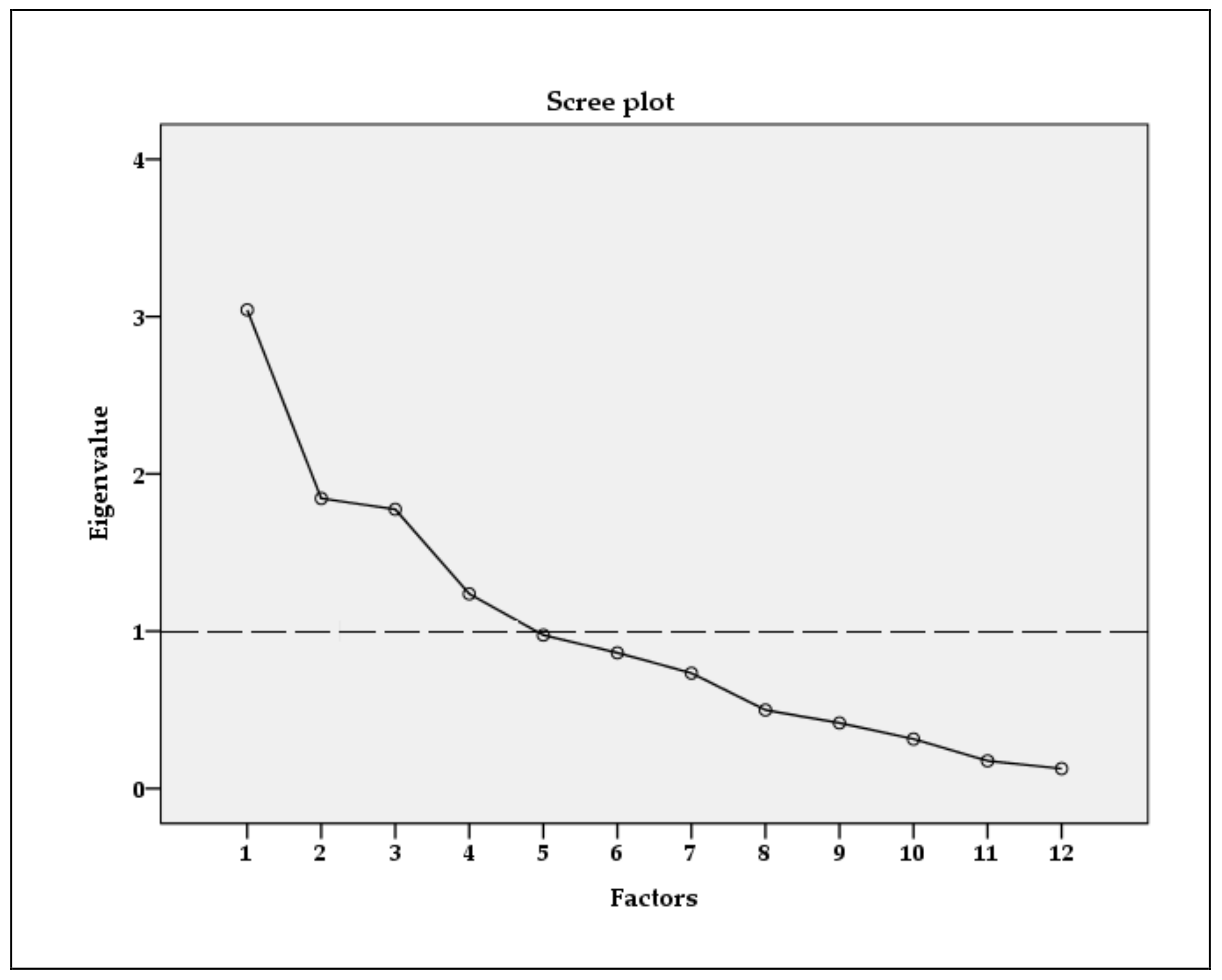
We applied PCA to categorize these 12 variables into a smaller set of factors. We also conducted several statistical analysis approaches to evaluate whether the variables we used were suitable for PCA. The Cronbach’s alpha measures the internal consistency. In other words, it means how close a variable is to other variables as a group. Generally, the acceptable threshold value of Cronbach’s alpha is 0.7. Subsequently, we also conducted the Kaiser–Meyer–Olkin (KMO) test to evaluate the quality of the correlations between variables. The acceptable threshold value is 0.6. We also applied Bartlett’s test of sphericity. This test examines whether the redundancy of all the variables can be represented with a few numbers of factors. If the p-value of Bartlett’s test of sphericity can reach a statistical significance level, it means the data set is suitable for PCA. In our study, the value of Cronbach’s alpha was 0.702. The KMO of PCA was 0.622. Also, Bartlett’s test of sphericity was highly significant (p-value < 0.05). These four components explained 65.7% of the total variables. Generally speaking, the result shows that our data set was acceptable for conducting PCA. Subsequently, according to Figure 3, the eigenvalues of the first four components are larger than 1. Moreover, the curve in Figure 3 shows a significant elbow start, which suggests that the PCA generates four principal components.
The first component includes Annual Income, Presidential Election Vote Rate, Number of Social-Civic Groups, Population with a College Diploma, and Population between 20 to 50 Years Old. The second component comprises the Capacity of Emergency Shelters, Number of Clinics, Number of Pharmacies. The third principal component includes the Number of Licensed Medical Personnel and Number of Hospital Beds. The last component includes the Number of Ambulances and Number of Emergency Services Stations. The first component (socioeconomic community) includes the social, community, and economic aspects of resilience. It explained 18.5% of all variables. The second component (fundamental medical) includes the part of the institutional and infrastructure resilience, which explained 19.7% of all variables. The third component (institutional) represents institutional resilience and explained 16.1% of all variables. The last component (infrastructure) stands for infrastructure resilience and explained 13.2% of all variables.
3.3. The Spatial Pattern of Components
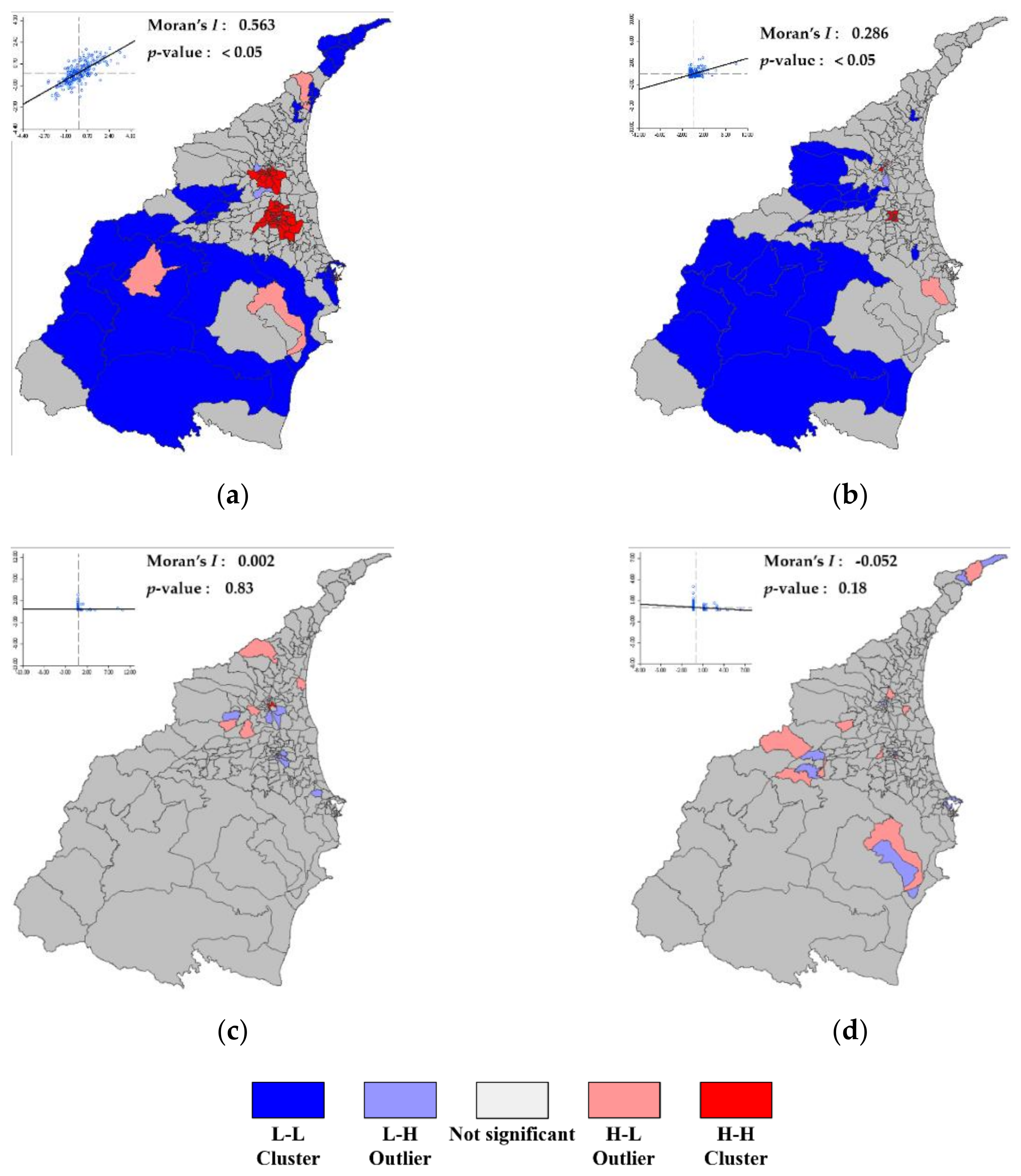
According to the spatial autocorrelation analysis for different components (Figure 4), we found the economic, community, and social resilience are highly correlated and cluster in plain areas, especially in urban areas such as Yilan City and Luodong Town. The reasons causing the uneven distribution are topography characteristics, accessibility, and the level of development. Compared to mountain areas, plain areas have a more significant advantage. After the completion of the freeway, the connection between our study site and Taipei stimulates economic development in plain areas. The fast growth of economics accompanies an advanced social and community status, such as a more robust social bond, political engagement, and higher education levels. Therefore, plain areas have higher socioeconomic community resilience. Furthermore, because of the better socioeconomic community conditions in plain areas, the demands for fundamental medical services also increase. Thus, fundamental medical services also cluster in plain areas. On the other hand, owing to the characteristics of the institution and infrastructure aspects, the distribution may not have a specific pattern. Most of the institutions and infrastructure are supposed to cover the entire area and serve all citizens. Therefore, it does not have a specific spatial pattern (justness of distribution).
3.4. BRIC
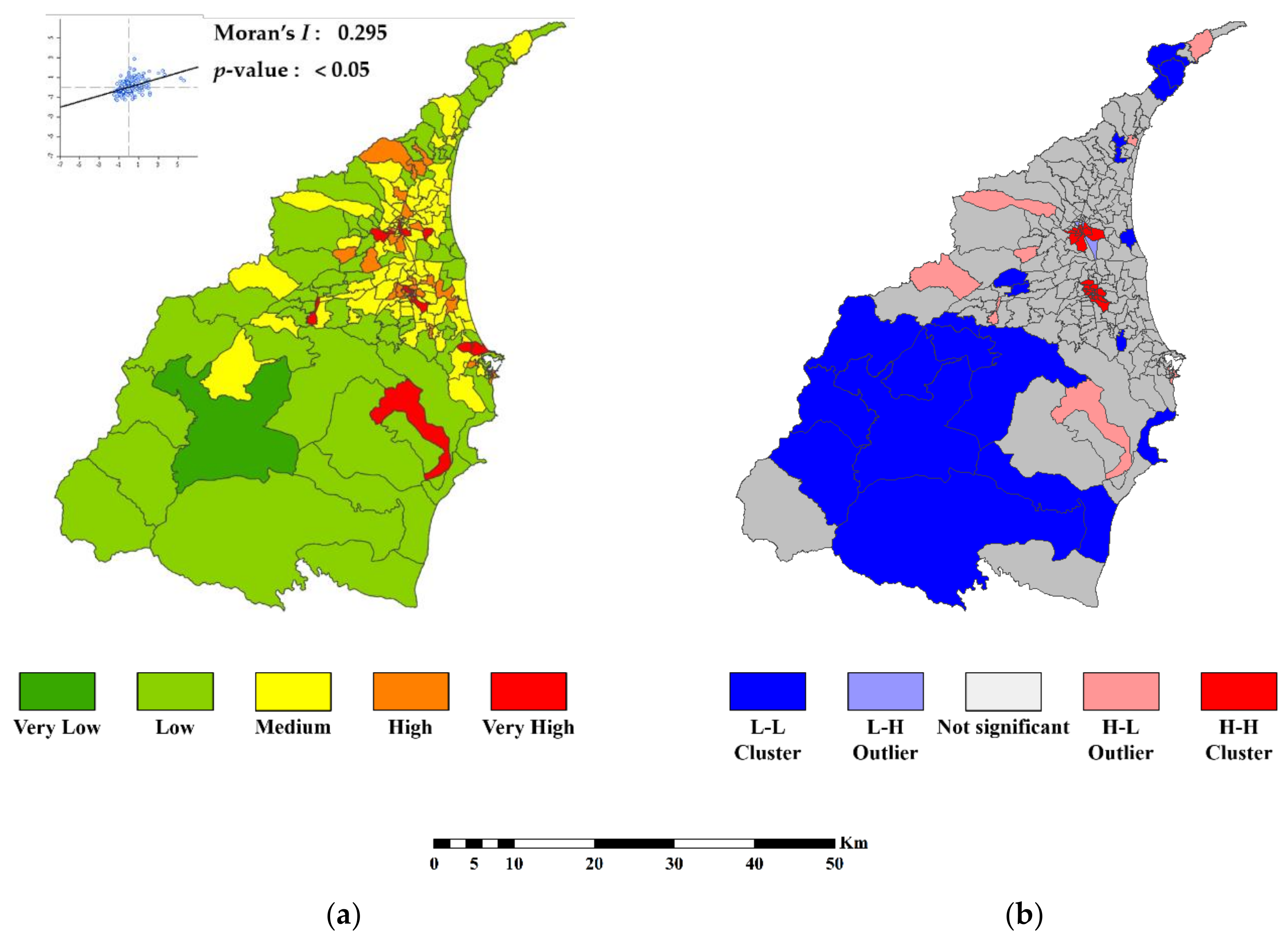
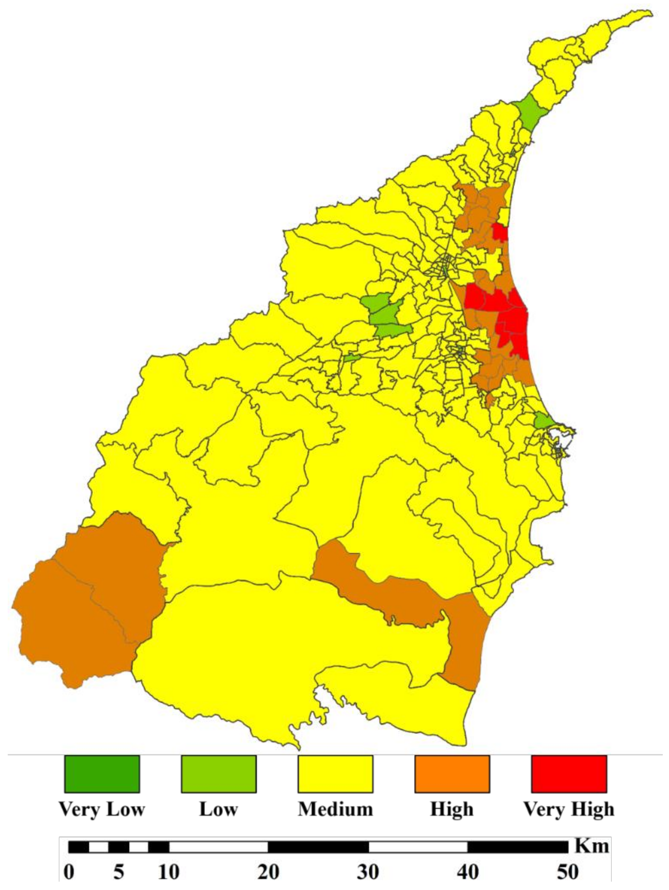
Finally, we aggregated all principal components into BRIC. In order to compare with the community within the study site, we also standardized the value we calculated. This approach allowed us to compare the BRIC value in each community with the mean value. Figure 5a shows the baseline resilience to natural hazards. Most of the plain areas are higher or equal to the average of baseline resilience, except parts of coastal areas, which are lower than the average. The number of communities with high or very high BRIC values is 52 (22%). Mountain areas, on the other hand, have significantly lower baseline resilience. The number of communities with low or very low BRIC values is 85 (36%). The reason causing the extremely uneven distribution is dominated by socioeconomic community resilience since the majority of communities in plain areas have higher socioeconomic community resilience. Besides, mountain areas do not have a suitable condition to develop. The topography characteristic increases the difficulty of development. As a result, the economy was not stimulated by the completion of the freeway. According to the result of the local spatial autocorrelation analysis in Figure 5b, all the H-H clusters are in plain areas, especially the urban region. On the other hand, in the mountain areas, most of the communities are L-L clusters. The key driver of the uneven distribution is socioeconomic community resilience.
In order to testify the effectiveness of the modified BRIC, we applied the GWR. Figure 6 shows the standardized prediction value. The spatial distribution of standardized prediction value fits with the dependent variable’s spatial distribution. Based on the similarity of the spatial distribution, the BRIC we built seems acceptable. In Table 2, we examine the model’s explanatory ability through the R2 and adjusted R2. The R2 of BRIC was 0.508, which means the explanatory ability is adequate. After taking account of the degree of freedom, the adjusted R2 was 0.316. Although the R2 and adjusted R2 can examine the explanatory ability, it cannot distinguish whether the indicator is biased or not. Thus, it is crucial to examine the spatial pattern of the standardized residual. If the standardized residual shows cluster spatially, it means that the indicator is biased. If the standardized residual is randomly distributed, it means that the indicator is unbiased. As a result, we applied spatial autocorrelation analysis to evaluate the spatial pattern of the standardized residual. The Moran’s I and p-value of the standardized residual were 0.087 and 0.031. The result of the spatial autocorrelation analysis shows that the spatial pattern is random. In other words, the BRIC we built is able to reflect the ground truth.
4. Discussion
Based on previous studies, we built the BRIC and modified it. In order to validate the effectiveness of the BRIC we built, we applied GWR to examine the indicator. The result of GWR shows the BRIC is unbiased and has an acceptable explanatory ability. In our study site, plain areas have relatively higher resilience than the rural areas, especially the urban region. In our case, the accessibility and topography characteristics both play an essential role in affecting the distribution of baseline resilience to natural hazards. The reason causing the urban region in plain areas to have better baseline resilience to natural hazards is owed to the better development of socioeconomic community resilience. Precisely, the accessibility and topography characteristics allow the development of economics and enable the plain areas to have high social, community, and economic resilience. The plain areas, compared to the mountain areas, are relatively close to the freeways, railroads, and harbor. Moreover, our study site lies along Taipei City, one of the largest and most prosperous cities in Taiwan. The highly accessible plain areas in Yilan County can easily attract the people who live in Taipei City. Recently, due to the completion of the high-speed railroad, more and more tourists from southwestern Taiwan have visited Yilan Country. The majority of these tourists spend most of their time and money in the tourist attractions in the plain areas, which also stimulated the development of a socioeconomic community in plain areas. Compared to the mountain areas, the topography also allows the people who live in plain areas to have an easier condition to develop. As for the mountain areas, the situation is different. Although the mountain areas have some of the major traffic routes, owing to the steep slope and narrow width, the traffic volume is far less than the traffic routes in plain areas. Moreover, major public transportation, the railroad, only passes through the plain areas. In other words, it will create obstacles if people want to develop mountain areas. Moreover, because of the steep slope and the intense precipitation during summer, the majority of the mountain areas are covered by the potential of debris flow. Even though there was no potential of debris flow, compared to the plain areas, the steep slope is another pullback for development. Thus, accessibility and topography characteristics strongly affect the distribution of baseline resilience to natural hazards.
Similar research has also done in the US. Nevertheless, the result is hugely different from our results. One of the most conclusive and interesting situations we found in this research is that urban regions such as Yilan City and Luodong Town urban areas dominate the resilience to natural hazards. This result is different from the previous research in the US [42,43]. Compared to our results, the metropolitan states in the US, such as the New England area, dominate economic resilience; nevertheless, the levels of community, institutional, and infrastructure resilience are relatively low. As a result, the metropolitan states do not have high resilience. A similar situation also occurs in California, where the majority levels of resilience are only medium to low resilience. On the other hand, the states such as Nebraska, Minnesota, Wisconsin, Iowa, and Dakotas did not have extremely high economic resilience like the metropolitan states. Nevertheless, the social, community, institution, and infrastructure resilience of these five states are higher than most of the metropolitan states. Despite the difference we mentioned, there is a similar situation that occurs in our research and the previous research in the US. Topography plays an essential role in affecting the resilience to natural hazards. In the US, the states located in intermountain western US and the Rocky mountain show a medium to very low resilience to natural hazards [42,43]. Our research also has similar results. Therefore, it is clear that the topography is an influential factor for affecting the resilience to natural hazards, no matter under which kind of spatial scale.
The institutional and infrastructure seems to be no influence in our study since it was randomly distributed. However, institutional and infrastructure resilience represent the capacity during the emergency response and recovery phase, which is also an important factor. The distribution of resources leads us to another issue. According to [1], the distribution is central to disaster management. “Distributive justice” refers to the justness of distribution, while “procedural justice” refers to the justness of the decision-making process. In our study site, the majority distribution of institutional and infrastructure resilience follows the concept of “distributive justice.” This approach promotes and focuses on the equal distribution of resources. This strategy can assure all citizens have an equal probability of obtaining the same assistance when encountering natural hazards. However, to some extent, this way also dilutes the resources. This system might encounter a fatal outcome if facing an extreme natural hazard, which creates damage that is more serious than the threshold of what each institution and infrastructure can take. On the other hand, if the distribution follows the rule of “procedural justice,” the resource will cluster in certain important areas, such as urban areas, and allow these areas to have a better chance to mitigate and adapt to the impact brought by natural hazards. Nevertheless, another article [60] argues that currently, the majority of resources are concentrated in urban areas. In this situation, some of the resources become overlapped and redundant, yet, the rural and indigenous areas have fewer emergency infrastructures and resources. Generally speaking, in this way, those areas with less or no resources will expose to a greater risk of natural hazards since the resources are distributed unevenly. In summation, different distribution patterns have different advantages and disadvantages. In our study site, owing to the equal distribution of institutional and infrastructure resilience, it is essential to have a regular assessment of the capabilities to set the acceptable thresholds [61,62,63,64]. In other words, a periodical assessment of baseline resilience to natural hazards is required. Our study provides an intuitive method to evaluate the baseline resilience to natural hazards, which also can be conducted periodically.
5. Conclusions
Resilience to natural hazards is an essential factor for humans to face escalating natural hazards in the future. The antecedent conditions, which are also known as baseline resilience to natural hazards of the system, are the key to investigating resilience to natural hazards. Owing to our special setting, we modified the BRIC. Nevertheless, BRIC is a highly adaptable indicator. Based on the result of GWR, the BRIC we built is valid. The spatial distribution shows that a part of our results is similar to previous studies. Most of the urban areas are the H-H cluster of BRIC, while most of the rural regions in the mountain areas are the L-L cluster of BRIC. This study found a different spatial pattern of resilience to natural hazards. In our case, the urban regions are far more resilient than the rural region, which is different from the previous research in the US. Moreover, we also found that the topography is a crucial factor. In our case and the previous research in the US, both show the mountain areas are low resilience areas. The topography has a significant and comprehensive influence on socioeconomic and community development, which affects the spatial pattern of resilience. Besides these findings, the spatial distribution pattern of institutional and infrastructural resilience also leads us to another critical discussion of resource distribution. In order to provide equal cover, the institutional and infrastructural resource usually follows “distributive justice”. This situation worsens the baseline resilience to natural hazards in mountain areas. Moreover, although “distributive justice” allows all communities to have equal opportunity to access the infrastructure and institutional resources, it might not be an efficient approach when encountering natural hazards. The “distributive justice” will dilute the resources.
The baseline resilience to natural hazards undoubtedly is highly connected to socioeconomic community development and resource distribution. However, both of these factors are highly related to topography. The effect of topography to baseline resilience to natural hazards is unneglectable. Furthermore, for future works, we will focus on the distribution approach. It is necessary to study whether we should follow “distributive justice” or “procedural justice”.
Author Contributions
Conceptualization, C.-H.S. and S.-C.L.; methodology, C.-H.S. and S.-C.L.; software, C.-H.S.; validation, C.-H.S.; formal analysis, C.-H.S. and S.-C.L.; investigation, C.-H.S. and S.-C.L.; resources, Sung, C.H.; data curation, C.-H.S. and S.-C.L.; writing—original draft preparation, C.-H.S. and S.-C.L.; writing—review and editing, C.-H.S. and S.-C.L.; supervision, S.-C.L. All authors have read and agreed to the published version of the manuscript.
Funding
This research received no external funding.
Conflicts of Interest
The authors declare no conflict of interest.
References
- Doorn, N. Resilience indicators: Opportunities for including distributive justice concerns in disaster management. J. Risk Res. 2015, 20, 711–731. [Google Scholar] [CrossRef] [Green Version]
- Intergovernmental Panel on Climate Change (IPCC). “Technical Summary.” Climate Change 2014: Impacts, Adaptation, and Vulnerability. Part A: Global and Sectoral Aspects. Contribution of Working Group II to the Fifth Assessment Report of the Intergovernmental Panel on Climate Change; Field, C.B., Barros, V.R., Dokken, D.J., Mach, K.J., Mastrandrea, M.D., Bilir, T.E., Chatterjee, M., Eds.; Cambridge University Press: Cambridge, UK, 2014. [Google Scholar]
- Winderl, T. Disaster Resilience Measurements: Stocktaking of Ongoing Efforts in Developing System for Measuring Resilience; UNDP: New York, NY, USA, 2014; pp. 18–29. [Google Scholar]
- Manyena, B.; Machingura, F.; O’Keefe, P. Disaster Resilience Integrated Framework for Transformation (DRIFT): A new approach to theorising and operationalising resilience. World Dev. 2019, 123, 104587. [Google Scholar] [CrossRef]
- Cutter, S.; Barnes, L.; Berry, M.; Burton, C.; Evans, E.; Tate, E.; Webb, J. A place-based model for understanding community resilience to natural disasters. Glob. Environ. Chang. 2008, 18, 598–606. [Google Scholar] [CrossRef]
- Klein, R.J.T.; Nicholls, R.J.; Thomalla, F. Resilience to Natural Hazards: How Useful Is this Concept? Environ. Hazards 2003, 5, 35–45. [Google Scholar] [CrossRef]
- Manyena, B. The concept of resilience revisited. Disasters 2006, 30, 434–450. [Google Scholar] [CrossRef]
- Cutter, S. The landscape of disaster resilience indicators in the USA. Nat. Hazards 2015, 80, 741–758. [Google Scholar] [CrossRef]
- Zhou, H.; Wang, X.; Wang, J. A Way to Sustainability: Perspective of Resilience and Adaptation to Disaster. Sustainability 2016, 8, 737. [Google Scholar] [CrossRef] [Green Version]
- Holling, C.S. Resilience and Stability of Ecological Systems. Annu. Rev. Ecol. Syst. 1973, 4, 1–23. [Google Scholar] [CrossRef] [Green Version]
- Prior, T.; Hagmann, J. Measuring resilience: Methodological and political challenges of a trend security concept. J. Risk Res. 2013, 17, 281–298. [Google Scholar] [CrossRef]
- Adger, W.N. Social Vulnerability to Climate Change and Extremes in Coastal Vietnam. World Dev. 1999, 27, 249–269. [Google Scholar] [CrossRef]
- Adger, W.N. Social and ecological resilience: Are they related? Prog. Hum. Geogr. 2000, 24, 347–364. [Google Scholar] [CrossRef]
- Adger, W.N.; Hughes, T.P.; Folke, C.; Carpenter, S.R.; Rockström, J. Social-Ecological Resilience to Coastal Disasters. Science 2005, 309, 1036–1039. [Google Scholar] [CrossRef] [Green Version]
- Carpenter, S.; Walker, B.; Anderies, J.M.; Abel, N. From Metaphor to Measurement: Resilience of What to What? Ecosystems 2001, 4, 765–781. [Google Scholar] [CrossRef]
- Folke, C. Resilience: The Emergence of a Perspective for Social-ecological Systems Analyses. Global Environ. Chang. 2006, 16, 253–267. [Google Scholar] [CrossRef]
- Gunderson, L. Ecological and Human Community Resilience in Response to Natural Disasters. Ecol. Soc. 2010, 15, 18–29. [Google Scholar] [CrossRef]
- Walker, B.; Holling, C.S.; Carpenter, S.R.; Kinzig, A. Resilience, Adaptability and Transformability in Social-ecological Systems. Ecol. Soc. 2004, 9, 5–13. [Google Scholar] [CrossRef]
- Barnett, J. Adapting to Climate Change in Pacific Island Countries: The Problem of Uncertainty. World Dev. 2001, 29, 977–993. [Google Scholar] [CrossRef] [Green Version]
- Norris, L.F.; Stevens, S.P.; Pfefferbaum, B.; Wyche, K.F.; Pfefferbaum, R.L. Community Resilience as a Metaphor, Theory, Set of Capacities, and Strategy for Disaster Readiness. Am. J. Community Psychol. 2007, 41, 127–150. [Google Scholar] [CrossRef]
- Cutter, S.; Burton, C.G.; Emrich, C.T. Disaster Resilience Indicators for Benchmarking Baseline Conditions. J. Homel. Secur. Emerg. Manag. 2010, 7, 1–22. [Google Scholar] [CrossRef]
- Jordan, E.; Javernick-Will, A. Indicators of Community Recovery: Content Analysis and Delphi Approach. Nat. Hazards Rev. 2013, 14, 21–28. [Google Scholar] [CrossRef]
- Twigger-Ross, C.; Coates, T.; Deeming, H.; Orr, P.; Ramsden, M.; Stafford, J. Community Resilience Research: Final Report on Theoretical Research and Analysis of Case Studies Report to the Cabinet Office and Defence Science and Technology Laboratory; Collingwood Environmental Planning Ltd.: London, UK, 2011. [Google Scholar]
- Manyena, S.B.; O’Brien, G.; O’Keefe, P.; Rose, J. Disaster resilience: A bounce back or bounce forward ability? Local Environ. 2011, 16, 417–424. [Google Scholar]
- Wardekker, A.; De Jong, A.; Knoop, J.M.; Van Der Sluijs, J.P. Operationalising a resilience approach to adapting an urban delta to uncertain climate changes. Technol. Forecast. Soc. Chang. 2010, 77, 987–998. [Google Scholar] [CrossRef] [Green Version]
- Prashar, S.; Shaw, R.; Takeuchi, Y. Assessing the resilience of Delhi to climate-related disasters: A comprehensive approach. Nat. Hazards 2012, 64, 1609–1624. [Google Scholar] [CrossRef]
- Pfefferbaum, R.L.; Pfefferbaum, B.; Van Horn, R.L.; Klomp, R.W.; Norris, F.H.; Reissman, D.B. The Communities Advancing Resilience Toolkit (CART). J. Public Health Manag. Pr. 2013, 19, 250–258. [Google Scholar] [CrossRef] [PubMed]
- Pfefferbaum, B.; Pfefferbaum, R.L.; Van Horn, R.L. Community resilience interventions: Participatory, assessmentbased, action-oriented processes. Am. Behav. Sci. 2015, 59, 238–253. [Google Scholar] [CrossRef]
- Cohen, O.; Leykin, D.; Lahad, M.; Goldberg, A.; Aharonson-Daniel, L. The conjoint community resiliency assessment measure as a baseline for profiling and predicting community resilience for emergencies. Technol. Forecast. Soc. Chang. 2013, 80, 1732–1741. [Google Scholar] [CrossRef]
- White, R.K.; Edwards, W.C.; Farrar, A.; Plodinec, M.J. A Practical Approach to Building Resilience in America’s Communities. Am. Behav. Sci. 2014, 59, 200–219. [Google Scholar] [CrossRef]
- Cox, R.S.; Hamlen, M. Community Disaster Resilience and the Rural Resilience Index. Am. Behav. Sci. 2014, 59, 220–237. [Google Scholar] [CrossRef]
- Wilkin, J.; Biggs, E.; Tatem, A.J. Measurement of Social Networks for Innovation within Community Disaster Resilience. Sustainability 2019, 11, 1943. [Google Scholar] [CrossRef] [Green Version]
- Cui, K.; Han, Z.; Wang, D. Resilience of an Earthquake-Stricken Rural Community in Southwest China: Correlation with Disaster Risk Reduction Efforts. Int. J. Environ. Res. Public Health 2018, 15, 407. [Google Scholar] [CrossRef] [Green Version]
- Cuthbertson, J.; Llanes, J.M.R.; Robertson, A.; Archer, F. Current and Emerging Disaster Risks Perceptions in Oceania: Key Stakeholders Recommendations for Disaster Management and Resilience Building. Int. J. Environ. Res. Public Health 2019, 16, 460. [Google Scholar] [CrossRef] [PubMed] [Green Version]
- Eisenman, D.; Chandra, A.; Fogleman, S.; Magana, A.; Hendricks, A.; Wells, K.; Williams, M.; Tang, J.; Plough, A. The Los Angeles County Community Disaster Resilience Project — A Community-Level, Public Health Initiative to Build Community Disaster Resilience. Int. J. Environ. Res. Public Health 2014, 11, 8475–8490. [Google Scholar] [CrossRef] [PubMed] [Green Version]
- Chun, H.; Chi, S.; Hwang, B.-G. A Spatial Disaster Assessment Model of Social Resilience Based on Geographically Weighted Regression. Sustainability 2017, 9, 2222. [Google Scholar] [CrossRef] [Green Version]
- Sherrieb, K.; Norris, F.H.; Galea, S. Measuring Capacities for Community Resilience. Soc. Indic. Res. 2010, 99, 227–247. [Google Scholar] [CrossRef]
- Sherrieb, K.; Louis, C.A.; Pfefferbaum, R.L.; Pfefferbaum, J.B.; Diab, E.; Norris, L.F. Assessing community resilience on the US coast using school principals as key informants. Int. J. Disaster Risk Reduct. 2012, 2, 6–15. [Google Scholar] [CrossRef]
- Peacock, W.G.; Brody, S.D.; Seitz, W.A.; Merrell, W.J.; Vedlitz, A.; Zahran, S.; Harriss, R.C.; Stickney, R. Advancing Resilience of Coastal Localities: Developing, Implementing, and Sustaining the Use of Coastal Resilience Indicators: A Final Report; Final report for NOAA CSC grant no. NA07NOS4730147; Hazard Reduction and Recovery Center: College Station/Houston, TX, USA, 2010. [Google Scholar]
- Yoon, D.K.; Kang, J.E.; Brody, S.D. A measurement of community disaster resilience in Korea. J. Environ. Plan. Manag. 2015, 59, 1–25. [Google Scholar] [CrossRef]
- Scherzer, S.; Lujala, P.; Rød, J.K. A community resilience index for Norway: An adaptation of the Baseline Resilience Indicators for Communities (BRIC). Int. J. Disaster Risk Reduct. 2019, 36, 101107. [Google Scholar] [CrossRef]
- Cutter, S.; Ash, K.; Emrich, C.T. The geographies of community disaster resilience. Glob. Environ. Chang. 2014, 29, 65–77. [Google Scholar] [CrossRef]
- Cutter, S.; Ash, K.; Emrich, C.T. Urban–Rural Differences in Disaster Resilience. Ann. Am. Assoc. Geogr. 2016, 106, 1236–1252. [Google Scholar] [CrossRef]
- Burton, C.G. A Validation of Metrics for Community Resilience to Natural Hazards and Disasters Using the Recovery from Hurricane Katrina as a Case Study. Ann. Assoc. Am. Geogr. 2014, 105, 67–86. [Google Scholar] [CrossRef]
- Pendall, R.; Foster, K.A.; Cowell, M. Resilience and regions: Building understanding of the metaphor. Camb. J. Reg. Econ. Soc. 2009, 3, 71–84. [Google Scholar] [CrossRef] [Green Version]
- Miles, S.B.; Chang, S.E. ResilUS: A Community Based Disaster Resilience Model. Cartogr. Geogr. Inf. Sci. 2011, 38, 36–51. [Google Scholar] [CrossRef]
- Frazier, T.G.; Thompson, C.M.; Dezzani, R.J.; Butsick, D. Spatial and temporal quantification of resilience at the community scale. Appl. Geogr. 2013, 42, 95–107. [Google Scholar] [CrossRef]
- Center Weather Bureau. Typhoon Database. Available online: https://rdc28.cwb.gov.tw/TDB/ (accessed on 5 February 2020).
- Directorate-General of Budget, Accounting and Statistics. STATDB. Available online: https://statdb.dgbas.gov.tw/pxweb/Dialog/statfile9.asp (accessed on 5 February 2020).
- Singh-Peterson, L.; Salmon, P.M.; Goode, N.; Gallina, J. Translation and evaluation of the Baseline Resilience Indicators for Communities on the Sunshine Coast, Queensland Australia. Int. J. Disaster Risk Reduct. 2014, 10, 116–126. [Google Scholar] [CrossRef]
- Cai, H.; Lam, N.S.-N.; Qiang, Y.; Zou, L.; Correll, R.M.; Mihunov, V.V. A synthesis of disaster resilience measurement methods and indices. Int. J. Disaster Risk Reduct. 2018, 31, 844–855. [Google Scholar] [CrossRef]
- Mayunga, J.S. Understanding and Applying the Concept of Community Disaster Resilience: A Capital-Based Approach. In Summer Academy for Social Vulnerability and Resilience Building; JOUR: Munich, Germany, 2007. [Google Scholar]
- Aldrich, D.P. Social, not physical, infrastructure: The critical role of civil society in disaster recovery. Disasters 2012, 36, 398–419. [Google Scholar] [CrossRef] [PubMed]
- Aldrich, D.P.; Meyer, M.A. Social Capital and Community Resilience. Am. Behav. Sci. 2014, 59, 254–269. [Google Scholar] [CrossRef]
- Ross, A.D. Local Disaster Resilience: Administrative and Political Perspectives; Routledge Press: New York, NY, USA, 2014. [Google Scholar]
- Moran, P.A.P. The Interpretation of Statistical Maps. J. R. Stat. Soc. Ser. B 1948, 10, 243–251. [Google Scholar] [CrossRef]
- Moran, P.A.P. Notes on continuous stochastic phenomena. Biometrika 1950, 37, 17–23. [Google Scholar] [CrossRef]
- Anselin, L. Local Indicators of Spatial Association-LISA. Geogr. Anal. 2010, 27, 93–115. [Google Scholar] [CrossRef]
- Fotheringham, A.S.; Charlton, M.; Brunsdon, C. Geographically Weighted Regression: A Natural Evolution of the Expansion Method for Spatial Data Analysis. Environ. Plan. A Econ. Space 1998, 30, 1905–1927. [Google Scholar] [CrossRef]
- Villagra, P.; Quintana, C. Disaster Governance for Community Resilience in Coastal Towns: Chilean Case Studies. Int. J. Environ. Res. Public Health 2017, 14, 1063. [Google Scholar] [CrossRef] [PubMed] [Green Version]
- Sen, A. Commodities and Capabilities; Oxford University Press: Cambridge, UK, 1985. [Google Scholar]
- Nussbaum, M.C. Women and Human Development; Cambridge University Press (CUP): Cambridge, UK, 2000. [Google Scholar]
- Gardoni, P.; Murphy, C. Recovery from natural and man-made disasters as capabilities restoration and enhancement. Int. J. Sustain. Dev. Plan. 2008, 3, 317–333. [Google Scholar] [CrossRef]
- Murphy, C.; Gardoni, P. The Acceptability and the Tolerability of Societal Risks: A Capabilities-based Approach. Sci. Eng. Ethics 2007, 14, 77–92. [Google Scholar] [CrossRef] [PubMed]
Figure 1.
The study site, Yilan County, is located in northeastern Taiwan. Yilan City and Luodong Township are the major urban areas in our study site. Owing to the location of Yilan County, over 30% of the typhoons striking Taiwan will have a direct impact on our study site.
Figure 1.
The study site, Yilan County, is located in northeastern Taiwan. Yilan City and Luodong Township are the major urban areas in our study site. Owing to the location of Yilan County, over 30% of the typhoons striking Taiwan will have a direct impact on our study site.

Figure 2.
The distribution of flood (a) and debris flow (b).

Figure 3.
The scree plot and eigenvalues of PCA. Based on the eigenvalues and scree plot, principal component analysis (PCA) generated four principal components.
Figure 3.
The scree plot and eigenvalues of PCA. Based on the eigenvalues and scree plot, principal component analysis (PCA) generated four principal components.

Figure 4.
Spatial pattern of principal component in community-scale: (a) socioeconomic community; (b) fundamental medical; (c) institutional; (d) infrastructure.
Figure 4.
Spatial pattern of principal component in community-scale: (a) socioeconomic community; (b) fundamental medical; (c) institutional; (d) infrastructure.


Figure 5.
The distribution and cluster map of BRIC in the community; (a) the spatial distribution and result of global spatial autocorrelation analysis; (b) the result of LISA and cluster map.
Figure 5.
The distribution and cluster map of BRIC in the community; (a) the spatial distribution and result of global spatial autocorrelation analysis; (b) the result of LISA and cluster map.

Figure 6.
The standardized value of prediction.


Table 1.
Variables and descriptive statistics.
| Variables | Mean | SD | Moran’s I | p-Value |
|---|---|---|---|---|
| Annual Income | 273,953.751 | 220,415.705 | 0.365 | <0.05 |
| Population With a College Diploma | 613.600 | 487.833 | 0.556 | <0.05 |
| Population Between 20 to 50 Years Old | 911.540 | 588.782 | 0.277 | <0.05 |
| Presidential Election Vote Rate | 0.636 | 0.041 | 0.388 | <0.05 |
| Number of Social-Civic Groups | 0.965 | 1.258 | 0.124 | <0.05 |
| Capacity of Emergency Shelters | 167.626 | 252.061 | 0.063 | 0.10 |
| Number of Clinics | 1.231 | 2.812 | 0.407 | <0.05 |
| Number of Licensed Medical Personnel | 10.596 | 74.772 | 0.017 | 0.41 |
| Number of Hospital Beds | 11.884 | 73.422 | −0.013 | 0.81 |
| Number of Pharmacies | 0.536 | 1.106 | 0.283 | <0.05 |
| Number of Emergency Services Stations | 0.086 | 0.310 | −0.068 | 0.12 |
| Number of Ambulances | 0.124 | 0.379 | −0.018 | 0.69 |
Note: SD, the standard deviation.
Table 2.
Summary and descriptive statistics of geographically weighted regression (GWR).
| Neighbors | R2 | Adjusted R2 | AICc | StdResid Moran’s I | p-Value |
|---|---|---|---|---|---|
| 45 | 0.508 | 0.316 | 626.696 | 0.087 | 0.031 |
Note: R2, Coefficient of determination; AICc, Akaike information criterion.
© 2020 by the authors. Licensee MDPI, Basel, Switzerland. This article is an open access article distributed under the terms and conditions of the Creative Commons Attribution (CC BY) license (http://creativecommons.org/licenses/by/4.0/).
Share and Cite
MDPI and ACS Style
Sung, C.-H.; Liaw, S.-C. A GIS Approach to Analyzing the Spatial Pattern of Baseline Resilience Indicators for Community (BRIC). Water 2020, 12, 1401. https://doi.org/10.3390/w12051401
AMA Style
Sung C-H, Liaw S-C. A GIS Approach to Analyzing the Spatial Pattern of Baseline Resilience Indicators for Community (BRIC). Water. 2020; 12(5):1401. https://doi.org/10.3390/w12051401
Chicago/Turabian StyleSung, Chien-Hao, and Shyue-Cherng Liaw. 2020. "A GIS Approach to Analyzing the Spatial Pattern of Baseline Resilience Indicators for Community (BRIC)" Water 12, no. 5: 1401. https://doi.org/10.3390/w12051401
Note that from the first issue of 2016, this journal uses article numbers instead of page numbers. See further details here.