Selection of Hydrological Probability Distributions for Extreme Rainfall Events in the Regions of Colombia

Abstract

Frequency analysis of extreme events is used to estimate the maximum rainfall associated with different return periods and is used in planning hydraulic structures. When carrying out this type of analysis in engineering projects, the hydrological distributions that best fit the trend of maximum 24 h rainfall data are unknown. This study collected maximum 24 h rainfall records from 362 stations distributed throughout Colombia, with the goal of guiding hydraulic planners by suggesting the probability distributions they should use before beginning their analysis. The generalized extreme value (GEV) probability distribution, using the weighted moments method, presented the best fits of frequency analysis of maximum daily precipitation for various return periods for selected rainfall stations in Colombia.

1. Introduction

Frequency analyses of extreme events are used to estimate maximum rainfall associated with different return periods [1,2,3], and their results are used to plan stormwater network projects, longitudinal dikes, overflows, drainage channels, cofferdams, gutters, circular and box culverts and bridges, among other infrastructure works [4,5]; they can also be used to carry out erosion analysis in hydrographic basins [6].

In recent years, due to the influence of global warming as well as changes in the magnitude and patterns of extreme precipitation events, it is necessary to periodically update the magnitudes of the maximum rainfall that are used to design hydraulic works [7]. In particular, extreme weather events such as floods, droughts and storms can increase in frequency over time [8,9,10]; thus, it is necessary to determine probability functions that best represent current trends in the data.

In Colombia, there are several meteorological factors that influence the climate and therefore the maximum precipitation over a 24 h period, among which are: (i) the relative position of subtropical high pressure centers, (ii) the equatorial convergence zone, (iii) the intertropical front, (iv) the prevailing winds, and (v) the effects of the local topography [11]. It is recommended that each region be analyzed (Andean, Caribbean, Pacific, Orinoquía and Amazonas) to take into account the geographic variability in maximum precipitation. The Institute of Hydrology, Meteorology and Environmental Studies (Instituto de Hidrología, Meteorología y Estudios Ambientales - IDEAM) is the governmental entity in Colombia that operates and manages the maximum 24 h rainfall records. However, regional autonomous corporations are also responsible for compiling hydroclimatological records.

When carrying out projections of maximum rainfall associated with specific return periods, it is necessary to perform frequency analysis [12,13,14]. In frequency analysis of extreme precipitation events, the hydrological probability distribution that best represents the trend of maximum 24 h rainfall data can be determined using functions such as the generalized extreme value (GEV) [15], Gumbel [1,3,13], log-Pearson type III [1,16], normal [3] and Pearson type III [17]. The parameters of the probability distributions are determined mainly by applying the method of maximum likelihood (ML) or the method of weighted moments (WM) [3,18]. To select the probability distribution function that best fits the trend of the data, different goodness of fit tests are usually used, such as the chi-square test or the Kolmogorov-Smirnov test [19,20,21]. The ML method uses a lot of calculations for determining parameters of hydrological distributions. Despite, the WM method is simpler than the ML method; it provides a good accuracy in the estimation parameters. In this sense, Mahdi & Cenac [22] showed that the Gumbel probability distribution was fitted adequately using the WM method than the ML method. A similar analysis showed how the WM method predicted better the behavior of extreme values using the GEV and Log-Pearson Type III distributions than the ML method; however, the Log-Normal distribution with the ML method provides the best prediction [23]. The Log-Pearson III distribution uses the SAM method for estimating parameters of extreme values.

Typically, to design hydraulic structures, a return period must be selected that varies between 5 and 100 years depending on the importance of the structure. In Colombia, Resolution 0330 of 2017 [24] outlines the return periods that should be used for urban drainage projects, the Manual on Drainage Design for Highways [25] provides the values for road works, and international recommendations are often used for other types of structures. An inadequate selection of a hydrological distribution could oversize or undersize a hydraulic structure, then the current research provides a starting point for selecting hydrological distributions since there has not been any official recommendation.

However, the probability distribution that should be used to make the statistical projections is never known a priori [26]. Therefore, in this study, we analyzed 362 stations with 24 h maximum rainfall records distributed throughout Colombia. The most representative probability distributions in each region of Colombia were selected and analyzed using the Gumbel, log-Pearson type II, Pearson, normal and GEV distributions and the chi-squared goodness of fit test. This study can be used by designers and engineers to determine a priori the hydrological distribution that should be used in a particular project.

2. Case Study

Colombia was selected as a case study (Figure 1) to determine the hydrological distributions that best represent the trend in the maximum 24 h rainfall data. During the compilation of the maximum 24 h rainfall records in Colombia, the following aspects were taken into account for each station: a minimum recording period of 30 years, eliminating outliers, using the entire available recording period and ensuring that the stations were distributed throughout each of the five regions that make up Colombia (Caribbean, Pacific, Andean, Orinoquía and Amazonas).

Table 1. Number of stations in each region.

Region	Number of Rainfall Stations	Percentage of Used Rainfall Stations (%)	Location of Rainfall Stations by Departments of Colombia
Andean	250	69	Antioquía, Boyacá, Caldas, Cauca, Cundinamarca, Huila, Quindío, Risaralda, Santander, Tolima
Caribbean	59	16	Atlántico, Bolívar, César, Córdoba, Magdalena, San Ándres y Providencia, Sucre
Pacific	37	10	Valle, Cauca
Orinoquía	11	3	Arauca, Vichada, Meta, Casanare
Amazonas	5	2	Vaupés, Putumayo, Guaviare, Amazonas, Caquetá
Total	362	100	N/A

and Figure 2 show the number of stations analyzed in Colombia. The maximum 24 h rainfall records were obtained from the IDEAM (Institute of Hydrology, Meteorology and Environmental Studies), which is the more important database in Colombia for collecting rainfall records. The stations in each region were selected to ensure they were distributed over the entire study area and had at least 30 years of records.

The results of Table 1 show that the Andean region represents 69% of the stations compiled, the Caribbean region 16%, the Pacific region 10% and the Orinoquía and Amazonas regions 3% and 2%, respectively. It is important to bear in mind that the regions with the lowest percentage of stations used in the present study (Orinoquía and Amazonas) also have the fewest stations installed.

Appendix A shows the codes of the stations with maximum 24 h rainfall data. Figure 2 shows the distribution of the stations used in each region of Colombia.

3. Methodology

The methodology used to determine the hydrological distribution that best represents the trends in 24 h maximum rainfall data associated with different return periods is presented as follows.

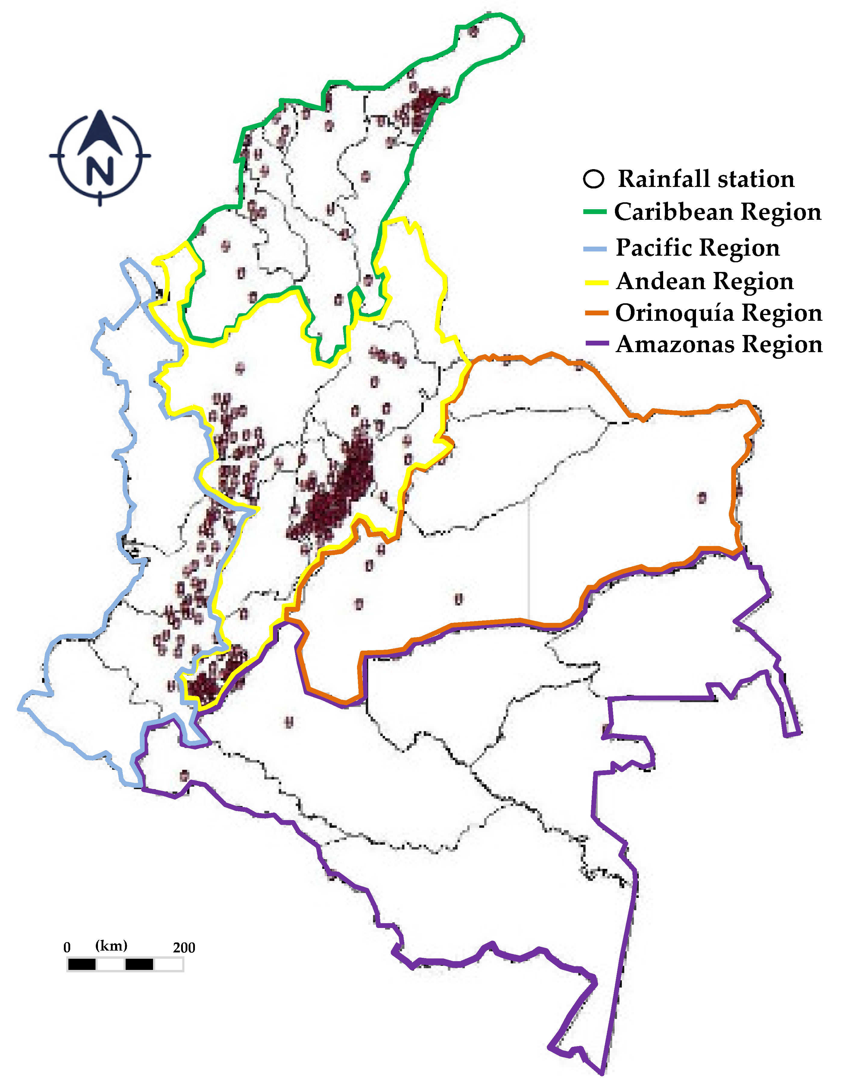
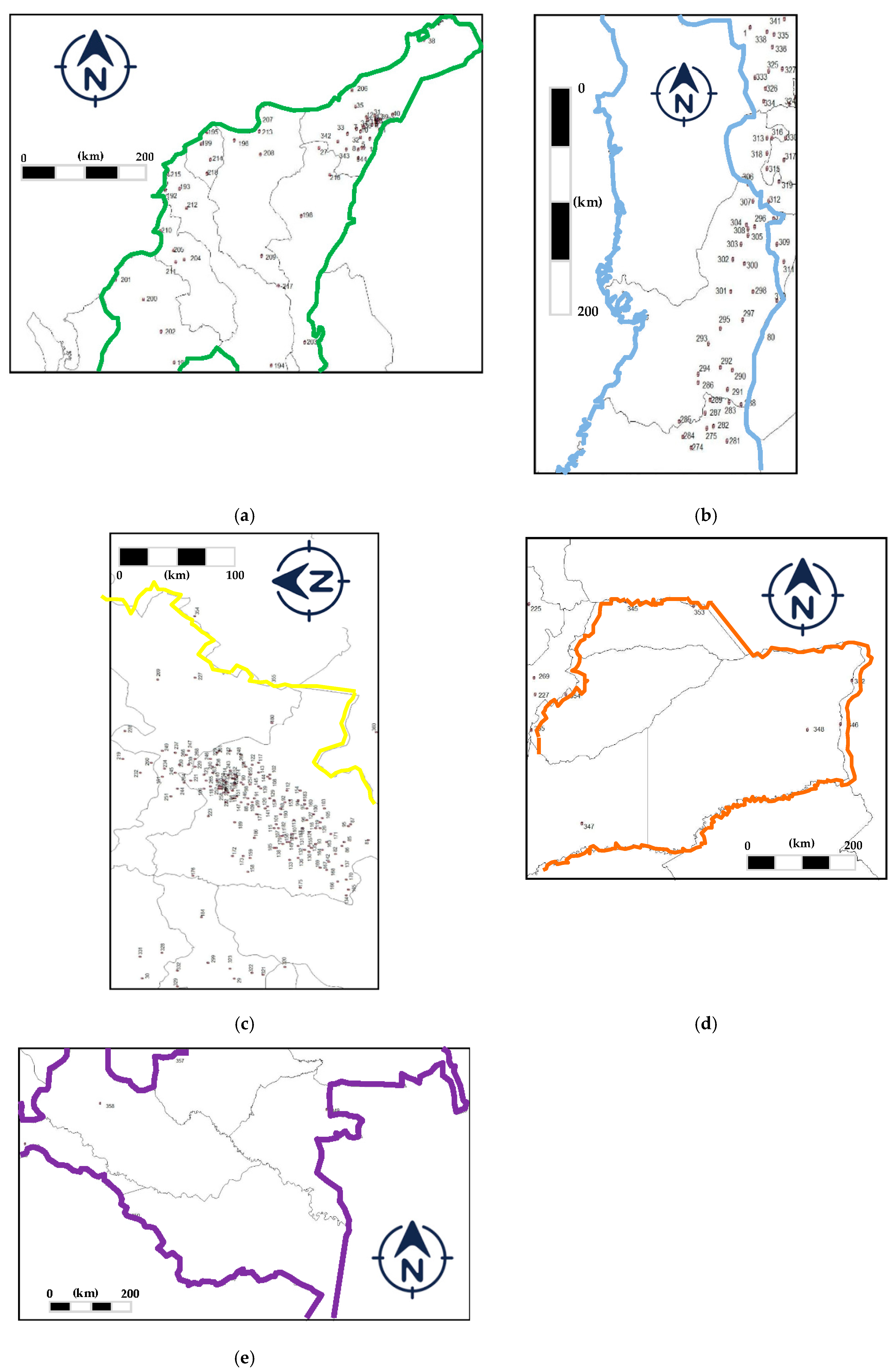
3.1. Selection of Rainfall Stations

The 24 h maximum rainfall records were collected from 362 rainfall stations distributed across Colombia (see Appendix A). Once the 362 stations with maximum rainfall records were selected, the error percentage of the selected stations with respect to the total installed stations in Colombia was 7determined. The equation used for a finite population is shown below [27]:

$$e=\sqrt{\frac{\frac{N{z}_{\alpha }^{2}pq}{n}-z_{\alpha }^{2}pq}{N-1}}$$

(1)

where

n = sample size, compiled from 362 stations;

N = population size, of 2977 stations installed by IDEAM;

$\alpha$ = the level of confidence chosen, assumed at 95%;

${\mathrm{Z}}_{\mathsf{\alpha }}$ = z value (where z is a normal centered and reduced variable), which leaves a proportion of the individuals out of the interval ±${\mathrm{Z}}_{\mathsf{\alpha }}$;

p = proportion at which the variable studied occurs in the population;

q = 1 − p. The most critical condition was assumed (p = q = 0.5);

e = estimation error.

Taking into account each of the previous variables, an estimation error of 4.83% was obtained.

3.2. Frequency Analysis

For each of the 362 stations, the annual series of maximum precipitation values was adjusted over 24 h with the Gumbel, GEV, Log-Pearson, Pearson and Normal probability distributions using the Hyfran Version 1.1 program [28].

• Gumbel distribution

The Gumbel distribution has typically been used to adjust the maximum 24 h precipitation values for different return periods. Parameters of this function are determined based on the recorded data. Its probability density function is given by:

$$f\left(x\right)=\frac{1}{\propto }{\mathrm{e}}^{\left[-\frac{\mathrm{x}-\mathrm{u}}{\propto }-{\mathrm{e}}^{-\frac{\mathrm{x}-\mathrm{u}}{\propto }}\right]}$$

(2)

where

$f\left(x\right)$: probability density function

$x$: random variable

u: mean of the data

$\propto$: scale parameter

• GEV distribution

The generalized extreme value distribution is widely used by hydrologists worldwide and in Colombia due to its versatility.

$$f\left(x\right)=\frac{1}{\propto }{\left[1-\frac{\mathrm{k}}{\propto }\left(\mathrm{x}-\mathrm{u}\right)\right]}^{\frac{1}{\mathrm{k}}-1}{\mathrm{e}}^{-{\left[1-\frac{\mathrm{k}}{\propto }\left(\mathrm{x}-\mathrm{u}\right)\right]}^{1/\mathrm{k}}}$$

(3)

where

k: shape parameter.

If k = 0, then the Gumbel distribution is obtained (see Equation (2)).

• Pearson type III distribution

This distribution is characterized by taking the gamma function to perform the frequency analysis and has three parameters that must be determined when performing the probabilistic adjustment.

$$f\left(x\right)=\frac{1}{|\propto |\mathsf{\gamma }\left(\mathrm{k}\right)}{\left(\frac{\mathrm{x}-\mathsf{\beta }}{\propto }\right)}^{\mathrm{k}-1}{\mathrm{e}}^{\left[-\left(\frac{\mathrm{x}-\mathsf{\beta }}{\propto }\right)\right]}$$

(4)

where

$\mathsf{\gamma }$: gamma function.

$\mathsf{\beta }$: location parameter.

• Log-Pearson type III distribution

By taking the natural logarithm of the Pearson type III distribution, the following distribution is obtained, which also consists of three parameters:

$$f\left(x\right)=\frac{1}{|\propto |\mathrm{x}\mathsf{\gamma }\left(\mathrm{k}\right)}{\left[\frac{\mathrm{lnx}-\mathsf{\beta }}{\propto }\right]}^{\mathrm{k}-1}{\mathrm{e}}^{\left[-\frac{\mathrm{lnx}-\mathsf{\beta }}{\propto }\right]}$$

(5)

• Normal distribution

The Normal distribution can be applied for estimating maximum daily precipitation for several return periods:

$$f\left(x\right)=\frac{1}{\sigma \sqrt{2\pi }}{e}^{\left\{-\frac{{\left(x-\mu \right)}^2}{2{\sigma }^2}\right\}}$$

(6)

where,

$\sigma$ and $\mu$ are the parameters of the distribution.

3.3. Goodness of Fit Test and Methods of Estimation of Parameters

The chi-squared test was used as a measure of goodness of fit to evaluate whether the probability distribution adequately fit the trend of the data.

$$X^2=\frac{{{\displaystyle \sum }}_i^n{\left(R_i-M_i\right)}^2}{M_i}$$

(7)

where

$X^2$: value of the chi-square test,

$R_i$: recorded value,

$M_i$: modeled value.

To adjust the parameters of each probability function, the methods of the ML, WM, and SAM were employed using the Hyfran program.

The methods of estimation of parameters were used for the following hydrological distributions: the GEV distribution, the ML and WM; the Gumbel distribution, the ML and WM; the Pearson Type III distribution, the ML and WM; the Log-Pearson Type III distribution, the SAM; and the Normal, the ML.

3.4. Selection of Hydrological Distribution

To select the best hydrological distribution the following analysis was conducted:

• For each rainfall stations the mean, maximum and minimum values, and standard deviation of the chi-squared test were computed for the Gumbel-ML, Gumbel-MV, Log-Pearson Type III-SAM, Pearson Type III-ML, Pearson Type III-WM, Normal-ML, GEV-ML and GEV-WM. These eight methods were used because they have adequately fitted the trend of maximum daily precipitation in various publications [22,23]. Based on this analysis, a regional mean value of the chi-squared test for Colombia was calculated based on the number of stations using a weighted mean.
• Estimation of percentage that establishes times where a hydrological distribution reaches the best fits of the trend of maximum daily precipitation records considering the minimum value of the chi-squared test.

4. Analysis of Results

This section presents the results that determine which probability density function best fits the 24 h maximum rainfall data of the 362 stations located in Colombia and should therefore be included in the maximum precipitation projections associated with different return periods. The error percentage of the selected rainfall stations was computed using Equation (1), obtaining a value of 4.83% based on the total number of rainfall stations of the IDEAM database.

Taking into account the methodology previously presented, the results presented in

Table 2. Adjustments for the hydrological probability distribution.

Region	Sta.	Probability Distribution
		Gum ML	Gum WM	LP SAM	Pea ML	Pea WM	Nor ML	GEV ML	GEV WM
		Values of the Chi-Squared Test
Andean	Me	5.85	5.63	6.40	45.01	7.09	8.04	5.11	4.60
	Mx	24.60	25.78	273.0	360.0	252.0	64.9	27.6	18.2
	Mn	0.26	0.26	0.36	0.26	0.29	0.29	0.29	0.29
	Sd	4.30	4.13	18.55	77.43	17.89	7.63	4.05	3.52
Caribbean	Me	7.72	5.64	16.81	91.57	6.34	7.41	5.41	5.18
	Mx	26.12	20.61	287.0	392.0	27.22	42.5	12.9	14.8
	Mn	0.43	0.74	0.89	0.89	0.50	0.89	0.89	0.50
	Sd	5.08	3.72	50.57	111.0	4.67	6.35	3.04	3.48
Pacific	Me	9.85	8.89	9.06	48.21	8.16	9.87	8.13	7.52
	Mx	22.42	25.52	20.40	280.0	24.89	23.9	17.8	16.4
	Mn	1.66	1.46	0.92	0.80	0.80	2.00	0.80	1.20
	Sd	5.25	6.00	5.19	91.97	5.47	5.97	4.44	4.26
Orinoquía	Me	13.91	8.09	33.49	102.1	7.35	9.24	8.89	6.31
	Mx	34.48	16.62	252.0	252.0	20.97	20.9	31.6	13.7
	Mn	4.15	2.42	2.64	4.11	3.00	3.68	1.50	1.50
	Sd	9.06	3.99	72.82	101.1	5.31	5.60	9.03	3.83
Amazonas	Me	6.64	6.32	87.14	183.0	4.93	6.70	4.37	4.36
	Mx	15.50	17.62	416.0	416.0	7.50	11.7	7.00	7.50
	Mn	1.60	0.92	1.46	4.00	1.46	0.38	1.46	1.46
	Sd	5.83	6.71	183.9	171.1	2.28	4.09	2.24	2.70
Regional mean for Colombia based on the number of stations	Me	6.82	6.05	10.31	56.57	7.06	8.14	5.57	5.04
Conventions Sta.: Statistic Me: mean Mx: maximum Mn: minimum Sd: standard deviation				Gum: Gumbel LP: Log-Pearson III Pea: Pearson III Nor: Normal GEV: Generalized extreme value			ML: Maximum likelihood WM: Weighted moments SAM: SAM method

were obtained. The results should be interpreted in a way that allows planners to know a priori the hydrological distributions that can occur in the regions of Colombia to save calculation time.

Based on the results in

Table 3. Values of chi-squared test for a sample of rainfall stations.

Station	Code	Region	Gum ML	Gum WM	LP SAM	Pea ML	Pea WM	Nor ML	GEV ML	GEV WM
Doña Juana	2120630	Andean	2.79	1.53	1.53	1.53	1.53	3.42	1.53	1.53
Apto Rafael Núñez	1401502	Carribean	7.71	7.71	7.43	7.43	4.57	7.14	7.14	7.71
El Placer	2610069	Pacific	5.51	3.87	7.56	7.97	5.92	19.87	9.21	7.56
Santa Rita	3306001	Orinoquía	10	7.00	5.00	168.00	5.00	5.00	7.00	5.50
Puerto Asis	4701003	Amazonas	15.5	5.46	416	416	5.46	6.15	5.46	5.46

the following can be deduced:

• In all regions of Colombia, the best fits of the chi-squared test were obtained with the GEV probability distribution. The weighted moment method best fits the parameters for this distribution and has an average regional value for Colombia of 5.04. There are other probability distributions that also fit the trend of the data similarly well: GEV with the maximum likelihood method, Gumbel with the weighted moment and maximum likelihood methods and Pearson’s with the method of weighted moments. The Gumbel distribution using the WM method brings a better estimation of maximum daily precipitation for several return periods in comparison with the ML, obtaining a similar result reported in the literature [22].
• In Colombia, the poorest fits were obtained when employing the Pearson type III probability distribution with the maximum likelihood method, where an average value of the chi-square test of 56.57 was obtained, and the log-Pearson type III distribution with the SAM method which had a value of 10.31. This finding is also verified by analyzing the maximum and minimum values and the standard deviation in these probability functions.
• In the Amazonas region, the best fit in the chi-squared test was obtained with the GEV probability distribution and the weighted moment method, with a value of 4.36. This value may have been obtained because few stations were used in the analyses.

Table 3 shows values of chi-squared test for a sample of rainfall stations in Colombia in order to show how a hydrological distribution is selected in each rainfall station. The green cells represent the obtained minimum values that best fits a hydrological distribution. It is of utmost important to mention that a rainfall station can be represented by various hydrological distributions, for instance, Doña Juana rainfall station (Andean region) can be simulated using the Gum-WM, LP-SAM, Pea-ML, Pea-WM, GEV-ML, and GEV-WM since these present a chi-squared value of 1.53.

Table 4. Selection of a hydrological distribution based on the minimum value of chi-squared test.

Region	Total Used Rainfall Stations	Reached Percentage of Hydrological Distributions
		GEV	Gum	Pea	LP	Nor
Andean	250	52%	36%	31%	28%	22%
Caribbean	59	44%	42%	32%	20%	27%
Pacific	37	54%	30%	43%	19%	22%
Orinoquía	11	73%	18%	36%	27%	27%
Amazonas	5	40%	60%	60%	20%	20%
Total	362	52%	36%	33%	25%	23%

shows, for a hydrological distribution, the best agreement using the minimum value of the chi-squared test considering the ML, MP, or SAM methods, which are marked in blue cells. Andean, Caribbean, Pacific, and Orinoquía regions were adjusted appropriately by the GEV distribution (using ML or WM method) with percentages of 52, 44, 54, and 73%, respectively, which implies the percentage of rainfall stations where the GEV distribution reaches the minimum value of chi-squared test (best agreement). The Gumbel and Pearson Type III fit adequately the parameters in the Amazonas region with a value of 60%. The GEV distribution presents the best fit with an overall value of 52%. Results are in agreement with the study conducted by Gonzalez-Alvarez et al. (2019) for the Caribbean region [24].

Since the Gumbel distribution corresponds to the scenario when the parameter k = 0 for the GEV distribution, then the percentage when both the Gumbel and GEV distribution is achieved using ML and WM methods is shown in

Table 5. Percentages for GEV and Gumbel distributions.

Region	Total Used Rainfall Stations	GEV and Gum
Andean	250	74%
Caribbean	59	73%
Pacific	37	73%
Orinoquía	11	82%
Amazonas	5	60%
Total	362	74%

. According to the analyzed sample, the 74% of rainfall stations in Colombia can be simulating using these hydrological distributions since the minimum values of the chi-squared test are reached.

To know the actual ranges of maximum daily precipitation for various return periods and the spatial variability in each region, the GEV distribution was applied to the analyzed rainfall stations. A summary of extreme values is presented in

Table 6. Maximum daily precipitation for several return periods using the GEV distribution.

Region	Extreme Values	Return Period
		5 yr.	10 yr.	25 yr.	50 yr.	100 yr.
Andean	Min	37.4	39.6	41.3	42	42.6
	Max	147	173	218	259	242
Caribbean	Min	64.6	84.3	97.5	99.3	100
	Max	167	199	241	272	306
Pacific	Min	35.3	40.5	47.8	53.9	60.4
	Max	121	135	151	162	172
Orinoquía	Min	119	131	141	145	149
	Max	145	152	186	220	262
Amazonas	Min	124	134	144	150	154
	Max	139	158	183	200	217

. Considering a return period of 100 years, the minimum value is reached in Andean region with a value of 42.6 mm (gray cell); and the maximum value is obtained in Caribbean region reaching an extreme precipitation of 306 mm (green cell). It is important to mention that there are no rainfall stations located in all departments in each region: in Andean region, Manizales and Norte de Santander are missing; in Caribbean region, La Guajira; in Pacific region, Chocó and Nariño; and in the Amazonas region, Guainía.

5. Conclusions and Recommendations

To estimate the maximum daily rainfall associated with different return periods for a particular project, it is recommended that designers and planners use the following hydrological distributions: the GEV, with the weighted moments and maximum likelihood methods; the Gumbel, with weighted moments and maximum likelihood; and the Pearson, with weighted moments. It is of utmost important to note that the GEV hydrological probability distribution (weighted moments method) best fits the trend of the data in all regions of the country.

For future studies, it is recommended to collect more data in the Amazonas and Orinoquía regions and to apply other goodness of fit tests. Similarly, it is recommended to perform a similar analysis using distributions that analyze non-stationary trends to evaluate the impact of climate effects, where the changes over time of rainfall records can be identified. This kind of analysis should be implemented for all regions in Colombia.

References

- Chow, V.T.; Maidment, D.R.; Mays, L.W. Applied Hydrology; McGraw-Hill: Bogotá, Colombia, 1994. [Google Scholar]
- Frechet, M. Sur la loi de probabilité de l’ecart máximum (On the probability law of máximum values). Ann. de la Soc. Pol. de Math. 1927, 6, 93–116. [Google Scholar]
- Maidment, D. Handbook of Hydrology; Mc Graw-Hill: New York, NY, USA, 1992. [Google Scholar]
- Clarke, R.T.; Dias de Paiva, R.; Bertacchi, C. Comparison of methods for analysis of extremes when records are fragmented: A case study using Amazon basin rainfall data. J. Hydrol. 2009, 368, 26–29. [Google Scholar] [CrossRef]
- Bedient, P.B.; Huber, W.C. Hydrology and Floodplain Analysis. Prentice-Hall: Upper Saddle River, NJ, USA, 2002; pp. 168–224. [Google Scholar]
- Arnaez, J.; Lasanta, T.; Ruiz-Flaño, P.; Ortigosa, L. Factors affecting runoff and erosion under simulated rainfall in Mediterranean vineyards. Soil Tillage Res. 2007, 93, 324–334. [Google Scholar] [CrossRef]
- Gonzalez-Alvarez, A.; Coronado-Hernández, O.E.; Fuertes-Miquel, V.S.; Ramos, H.M. Effect of the Non-Stationarity of Rainfall Events on the Design of Hydraulic Structures for Runoff Management and Its Applications to a Case Study at Gordo Creek Watershed in Cartagena de Indias. Colomb. Fluids 2018, 3, 27. [Google Scholar] [CrossRef] [Green Version]
- Obeysekera, J.; Salas, J.D. Quantifying the uncertainty of design floods under nonstationary conditions. J. Hydrol. Eng. 2014, 19, 1438–1446. [Google Scholar] [CrossRef]
- Obeysekera, J.; Salas, J.D. Frequency of recurrent extremes under nonstationarity. J. Hydrol. Eng. 2016, 21, 04016005. [Google Scholar] [CrossRef]
- Yang, T.; Shao, Q.; Hao, Z.-C.; Chen, X.; Zhang, Z.; Xu, C.-Y.; Sun, L. Regional frequency analysis and spatio-temporal pattern characterization of rainfall extremes in the Pearl River Basin, China. J. Hydrol. 2009, 380, 386–405. [Google Scholar] [CrossRef]
- Nunn, Dwight. Ingetec, S.A-Empresa de Acueducto y Alcantarillado de Bogotá. In Estimating of Maximum Daily Precipitation of Tributaries of Bogotá River; Ingetec: Bogotá, Colombia, 1968.
- Pathak, C.S. Frequency analysis of rainfall maximums for Central and South Florida, Technical Publication EMA # 390. 2001. Available online: http://my.sfwmd.gov/portal/page/portal/pg_grp_tech_pubs/portlet_tech_pubs/ema-390.pdf (accessed on 12 March 2018).
- Gumbel, E.J. The return period of flood flows. Ann. Math. Stat. 1941, 2, 163–190. [Google Scholar] [CrossRef]
- Weibull, W. A statistical theory of the strength of materials. In Proceedings of the Ingeniors Vetenskaps Akademien (The Royal Swedish Institute for Engineering Research) No. 51, Stockholm, Sweden, 1 Januray 1939; 1939; pp. 5–45. [Google Scholar]
- Grego, J.M.; Yates, P.A. Point and standard error estimation for quantiles of mixed flood distribution. J. Hydrol. 2010, 391, 289–301. [Google Scholar] [CrossRef]
- Koutrouvelisa, I.A.; Canavos, G.C. A comparison of moment-based methods of estimation for thelogPearson type 3 distribution. J. Hydrol. 2000, 234, 71–81. [Google Scholar] [CrossRef]
- Xuewu, J.; Jing, D.; Shen, H.W.; Salas, J.D. Plotting positions for Pearson type-III distribution. J. Hydrol. 2003, 74, 1–29. [Google Scholar] [CrossRef]
- Makkonen, L. Problems in the extreme value analysis. Struct. Saf. 2006, 30, 405–419. [Google Scholar] [CrossRef]
- Kolmogorov, A.N. Sulla determinazione empirica di una legge di distribuzione. G. dell’Instituto Ital. degli Attuari 1933, 4, 83–91. [Google Scholar]
- Smirnov, N.V. Estimate of deviation between empirical distribution functions in two independent samples. Bull. Mosc. Univ. 1939, 2, 3–16. [Google Scholar]
- Smirnov, N.V. Table for estimating the goodness of fit of empirical distributions. Ann. Math. Stat. 1948, 19, 279–281. [Google Scholar] [CrossRef]
- Mahdi, S.; Cenac, M. Estimating Parameters of Gumbel Distribution using the Methods of Moments, Probability Weighted Moments and Maximum Likelihood. Rev. de Matemáticas Teoría y Apl. 2005, 12, 151–156. [Google Scholar] [CrossRef] [Green Version]
- Seckin, N.; Yurtal, R.; Haktanir, T.; Dogan, A. Comparison of Probability Weighted Moments and Maximum Likelihood Methods Used in Flood Frequency Analysis for Ceyhan River Basin. Arab. J. Sci. Eng. 2009, 35, 49–69. [Google Scholar]
- Ministerio de Vivienda, Ciudad y Territorio. República de Colombia. Resolution 0330 of 8 June 2017. Available online: http://www.minvivienda.gov.co/ResolucionesAgua/0330%20-%202017.pdf (accessed on 20 March 2020).
- Ministerio de Transporte, Instituto Nacional de Vías. República de Colombia. Manual on Drainage Design for Highways. 2009. Available online: https://www.invias.gov.co/index.php/archivo-y-documentos/documentos-tecnicos/especificaciones-tecnicas/984-manual-de-drenaje-para-carreteras/file (accessed on 20 March 2020).
- Gonzalez-Alvarez, A.; Viloria-Marimón, O.; Coronado-Hernández, O.E.; Vélez-Pereira, A.; Tesfagiorgis, K.; Coronado-Hernández, J. Isohyetal Maps of Daily Maximum Rainfall for Different Return Periods for the Colombian Caribbean Region. Water 2019, 11, 358. [Google Scholar] [CrossRef] [Green Version]
- Krishnamoorthy, K.; Peng, J. Some properties of the exact and score methods for binomial proportion and sample size calculation. Commun. Stat. Simul. Comput. 2007, 36, 1171–1186. [Google Scholar] [CrossRef]
- El Adlouni, S.; Bobée, B. Hydrological Frequency Analysis Using HYFRAN-PLUS Software. User’s Guide available with the software DEMO 2015. Available online: http://www.wrpllc.com/books/HyfranPlus/indexhyfranplus3.html (accessed on 20 March 2020).