A New Parallel Framework of SPH-SWE for Dam Break Simulation Based on OpenMP
by
 ,
,
Yushuai Wu
1, 
Lirong Tian
1,
Matteo Rubinato
2 ,
,
Shenglong Gu
1,3,*,
Teng Yu
1,
Zhongliang Xu
4,
Peng Cao
5,6,
Xuhao Wang
6,7 and
Qinxia Zhao
1 1
School of Water Resources and Electric Power, Qinghai University, Xining 810016, China
2
School of Energy, Construction and Environment & Centre for Agroecology, Water and Resilience, Coventry University, Coventry CV1 5FB, UK
3
State Key Laboratory of Plateau Ecology and Agriculture, Qinghai University, Xining 810016, China
4
Transportation Bureau, Haiyan County, Jiaxing 812200, China
5
College of Architecture and Civil Engineering, Beijing University of Technology, Beijing 100124, China
6
Qinghai University-Tsinghua University, Sanjiangyuan University, Sanjiangyuan Research Institute, Qinghai University, Xinning 810016, China
7
School of Highway, Chang’an University, Xi’an 710064, China
*
Author to whom correspondence should be addressed.
Water 2020, 12(5), 1395; https://doi.org/10.3390/w12051395
Submission received: 7 April 2020
/
Revised: 7 May 2020
/
Accepted: 8 May 2020
/
Published: 14 May 2020
(This article belongs to the Special Issue Advances in Modelling and Prediction on the Impact of Human Activities and Extreme Events on Environments)
Abstract
:Due to its Lagrangian nature, Smoothed Particle Hydrodynamics (SPH) has been used to solve a variety of fluid-dynamic processes with highly nonlinear deformation such as debris flows, wave breaking and impact, multi-phase mixing processes, jet impact, flooding and tsunami inundation, and fluid–structure interactions. In this study, the SPH method is applied to solve the two-dimensional Shallow Water Equations (SWEs), and the solution proposed was validated against two open-source case studies of a 2-D dry-bed dam break with particle splitting and a 2-D dam break with a rectangular obstacle downstream. In addition to the improvement and optimization of the existing algorithm, the CPU-OpenMP parallel computing was also implemented, and it was proven that the CPU-OpenMP parallel computing enhanced the performance for solving the SPH-SWE model, after testing it against three large sets of particles involved in the computational process. The free surface and velocities of the experimental flows were simulated accurately by the numerical model proposed, showing the ability of the SPH model to predict the behavior of debris flows induced by dam-breaks. This validation of the model is crucial to confirm its use in predicting landslides’ behavior in field case studies so that it will be possible to reduce the damage that they cause. All the changes made in the SPH-SWEs method are made open-source in this paper so that more researchers can benefit from the results of this research and understand the characteristics and advantages of the solution proposed.
1. Introduction
The Smooth Particle Hydrodynamics (SPH) is a meshless method [1] very commonly used nowadays [2,3,4,5,6,7,8,9,10,11,12]. Gingold and Monaghan [13] were the first to propose this method to solve astrophysical simulations, using statistical techniques to recover analytical expressions for the physical variables from a known distribution of fluid elements. The SPH method is typically used for solving the equations of hydrodynamics in which Lagrangian discretized mass elements are followed [14]. Compared with the limitations of the Eulerian grid method [15,16,17], the SPH method has unique advantages in dealing with free water surface and moving boundary conditions [18,19,20,21]. In fact, the SPH method strictly runs in accordance with the law of conservation of mass and can deal with free surface and moving boundary flexibly; hence, it is very suitable for simulating dam break flows [22].Flooding due to dam break has potentially disastrous consequences, and multiple studies were conducted to numerically replicate the hydrodynamics of this phenomenon [23,24,25,26,27,28]. In most cases, the dam break flow occurs in a wide area and lasts for a long time. Therefore, the Shallow Water wave Equations (SWEs) have become the main application formulae for this specific dam break problem.
In 1999, Wang and Shen [29] applied the SPH method to SWEs for the first time. Dam break flows are unsteady open channel flows that can be described by the St. Venant equations, which are equations that can be used for flows with strong shocks [29]. The study conducted by Wang and Shen [29] has demonstrated that the method developed based on the SPH is capable of providing accurate simulations for mixed flow regimes with strong shocks. In 2005, Ata and Soulaimani [30] tried to reduce the difficulties that were associated with the treatment of the solid boundary conditions, especially with irregular boundaries. Ata and Soulaimani [30] derived a new artificial viscosity term by using an analogy with an approximate Riemann solver, and the several numerical tests conducted have confirmed that the stabilization proposed provides more accurate results than the standard artificial viscosity introduced by Monaghan [22]. However, Ata and Soulaimani [30] found that it was difficult to implement the Dirichlet boundary conditions for bounded domains. Different techniques such as symmetrization and ghost particles were implemented; nevertheless, results obtained for irregular boundaries or in presence of shocks were not satisfactory, and there was a need to make SPH method more competitive with standard approaches [30].
A new method with good stability was then needed for the SPH numerical simulation of shallow water equations to deal with dam break flows, flood waters, debris flows, avalanches, and tidal waves.
De Leffe et al. [31] proposed an improved calculation method based on a two-dimensional SPH solid wall boundary condition. By introducing a periodic redistribution of the particles and using a kernel function with variable smoothing length, this modification was tested and validated against dam break flows on a flat dry bottom in 1D and 2D. Comparisons conducted against literature results [30,32,33] have confirmed how this new approach is robust and able to simulate complex hydrodynamic situations.
However, to date, only a few studies have investigated the efficiency of solving the SPH-SWEs model. Vacondio et al. [34,35,36,37] have developed the serial code to solve the SWEs by using the SPH method and have made an open source version called SWE-SPHysics, which has been optimized and adapted based on the hydrodynamics investigated by other researchers [38,39,40,41,42,43,44,45,46,47,48,49,50,51,52]. Despite continuous progress, there is still a limitation related to the computational efficiency when the number of particles to simulate is very large, and this aspect still needs to be improved.
Xia and Liang [53] explored the Graphic Processing Units (GPUs) to accelerate an SPH-SWE model for wider applications such as dam breaks. Xia and Liang [53] demonstrated that the performance of the new GPU accelerated SPH-SWE model can significantly improve the calculation efficiency and verified that the quadtree neighbor searching method may reduce redundant computation when searching neighbor particles [53]. Furthermore, Liang et al. [54] developed a shock-capturing hydrodynamic model to simulate the complex rainfall-runoff and the induced flooding process in a catchment in England, Haltwhistle Burn, of 42 km2, and implemented it on GPUs for high-performance parallel computing.
GPU has been enhanced with a Fortran programming language capability employing CUDA (Compute Unified Device Architecture), known as CUDA Fortran [55]. Although the GPU parallel computing performance is strong, the GPU price is relatively expensive and support for the CUDA FORTRAN language compiler is limited. Furthermore, if CUDA FORTRAN language is compared with other parallels (OpenMP and MPI), the program design is also more complex [56,57,58].
Over the years, with the development of parallel computing, the development of OpenMP and MPI in parallel methods has matured, and MPI is widely used in the field of engineering computing [59,60,61,62,63]. However, in this multi-machine cluster environment, memory is not shared. For global shared data operations, data must be transferred by the communication between machines [64,65].
OpenMP is based on the shared storage mode of multi-core processors, and it is commonly used in parallel processing of single workstations. Although it is limited by the processing capacity and memory capacity of a single node, it can simplify the past multi-core computing to the present multi-core computers. The program design is relatively simple, and it can secure the advantages of economic and programming optimizations [66].
Therefore, this paper adopts the parallel computing method of CPU-OpenMP that is applied to a single machine and a multi-core to calculate the new SPH-SWEs framework for the parallel computing of the test case of 2-D dry-bed dam break with particle splitting [67,68] and a 2-D debris flow with a rectangular obstacle downstream the dam [2]. The accuracy of the new SPH-SWEs framework was then verified by comparing the serial algorithm, and the advantages of CPU-OpenMP parallel computing were analyzed.
The paper is organized as follows: Section 2 describes the methodology adopted presenting the theoretical derivation of the numerical model applied and the governing equations. Section 3 explains the setup of the SPH-SWEs method used. Section 4 provides the results of the application tested with a discussion of the results obtained. Lastly, Section 5 produces a brief summary and concluding remarks of the whole study.
2. Methodology
Ata et al., [30] and Paz and Bonet [32] have initiated the idea of SPH-SWE model solution, which is described in Section 2.1 with all the governing equations.
2.1. Governing Equations
By ignoring the Coriolis effect and the fluid viscosity, SWEs can be written in the Lagrangian form as follows:
d represents the water depth, g the acceleration of gravity, v is velocity, b represents the riverbed elevation, and Sf represents the riverbed friction. In the SWEs, the area density is defined as:
ρ represents the density, and ρw represents the density of water.
2.2. Water Depth Solutions
According to the SPH idea, the area density (i.e., water depth) of particles is solved as shown below in the implicit function:
xi/xj represents the particle coordinates; mj represents the particle mass of j; hi and ρi represent the smooth length and the area density of the particle i; h0 and ρ0 represent the initial values of the smooth length and the area density, respectively; dm represents the latitude (1 represents one dimension, 2 represents two dimensions) and W represents the kernel function.
2.3. Speed Solution
According to the Lagrangian equation of motion [69], ai is the acceleration of the particle i, and the solution formula of each particle can be obtained as follows:
represents b(x) of the curvature tensor [70]; represents the acceleration caused by the internal force; represents the riverbed gradient of the particle i, and in order to deal with any complex terrain problem, the riverbed gradient can be modified as follows [71,72]:
denotes the gradient of the modified kernel function, which is modified by the correction matrix Li, as shown below:
In order to reduce the numerical oscillation and ensure the stability of the calculation, one method is to increase the viscosity term as introduced below [73]:
β represents the correction coefficient caused by variable smooth length; rij represents the particle spacing; πij represents the numerical viscosity added to maintain stability. However, this method has the problem of numerical dissipation.
To reduce this issue, the interaction between two particles was treated as a Riemann problem [74], as follows:
dl and dr represent the water depth on the left and right sides, respectively; k = l and k = r represent the left and right states, respectively; d0 represents the initial estimated water depth; represents the shallow water wave velocity.
2.4. Time Integration and Boundary Processing
In order to update the particle velocity and displacement, the leap-frog time integration scheme [75] was used. By using this method, both time and space are of second-order accuracy, and the storage demand is relatively low, however the calculation efficiency is relatively high, as shown below:
Δt represents the time step; where the time step must meet the Courant number condition [76] displayed as follows:
To solve the boundary problem, this study adopts the Modified Virtual Boundary Particle (MVBP) method [36]. MVBP method is an improvement of the virtual boundary particle (VBP) method [77]. The virtual particles on the boundary will neither move with the fluid particles nor interact with them but generate the virtual particles similar to the mirror image through point symmetry. This method is easier and simpler in dealing with the complex boundary.
Compared with the VBP method, the MVBP method has two improvements: (1) When a virtual boundary particle is within the range of the kernel function of a fluid particle, two layers of newly generated virtual particles can be added (Xk,1 = 2Xv − Xi and Xk,2 = 4Xv − Xi). Among them, Xk,1 and Xk,2 represent the coordinates of the newly generated virtual particles, and Xv represents the virtual boundary particles; (2) When the internal angle of the boundary is less than or equal to 180°, two newly generated virtual particles are added outside the corner. Compared with the single point of the VBP method, this improvement reduces the kernel truncation error.
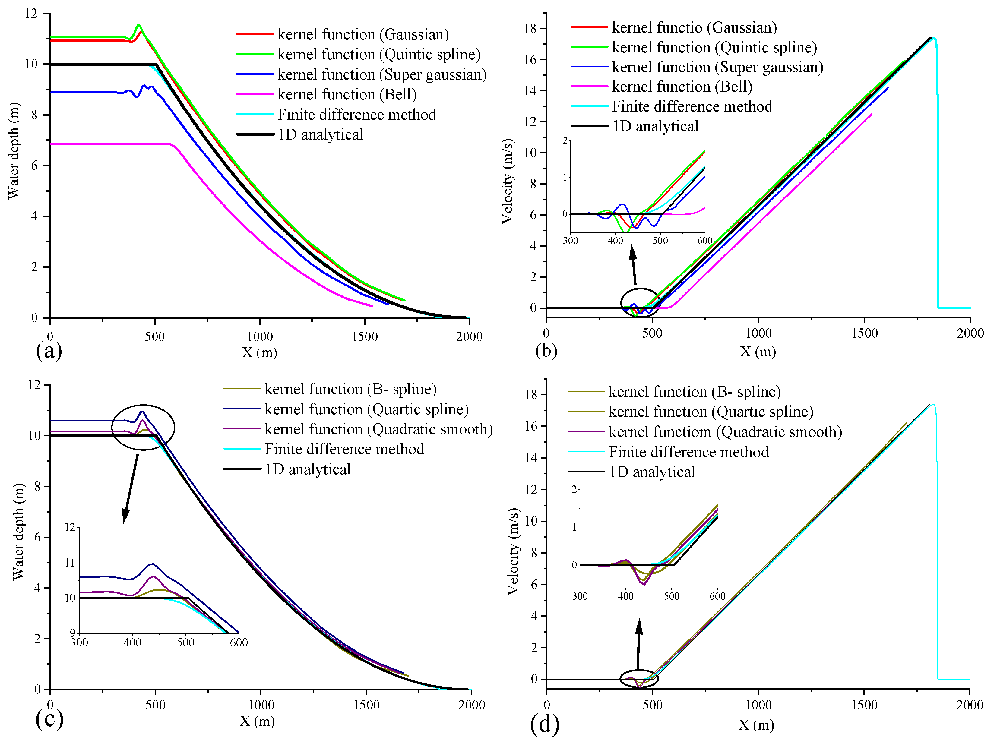
In order to verify the effect of different kernel functions to simulate the dam break, this paper used the SPH-SWE open source code [34,35,36,37,68] and applied different kernel functions (B-spline, super Gauss, quadratic spline, Gauss, quartic spline, quintic and Bell) to simulate case 2 open source scenario [68]. These were the initial conditions considered for the dam-break: (i) simulation area was 2000 m long; (ii) the river bed elevation was 0 m; (iii) the initial fluid particle area was 1000 m long; (iv) the particle spacing was 10 m; (v) the initial water depth was 10 m, (vi) and the simulation duration was 50 s. The position, the water depth, and speed of the fluid particles were obtained as an output every 10 s. After verification, the advantages and disadvantages of different kernel functions and different numerical oscillation processing methods (see Equations (7)–(8)) identified from the results are consistent. At t = 50 s, the water depth dissipated after 1500 m, and the results of different kernel functions and different numerical oscillation processing methods can be visually reflected through the graphs in Figure 1; at the same time, it also illustrates the continuity of the numerical oscillation issue. Therefore, the data of t = 50 s (Figure 1 results) was selected for analysis in this study.
It can be noticed from Figure 1 that in the numerical simulation of dam break based on SPH-SWEs approach, all kernel functions are characterized by numerical oscillation except the option where the Bell kernel function is considered. The three kernel functions that provide a more accurate estimation of the water depth and the velocity are B-spline, quadratric spline, and quartic spline (above 85.7%). Figure 2a–d shows the absolute error between the calculated water depths and velocities using these three kernel functions vs. the analytical solution. Results displayed confirm the optimal performance of the B-spline kernel function in dam break simulations.
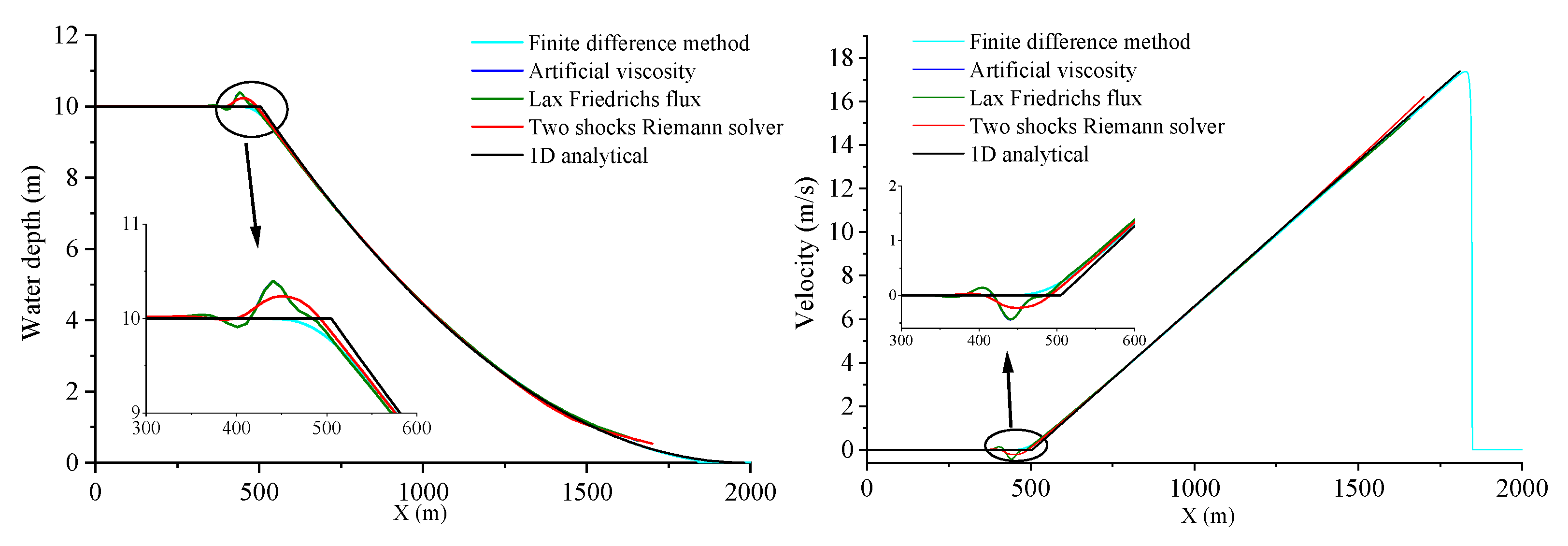
If the kernel function adopted is B-spline, the numerical oscillation is treated as adding the viscosity term (numerical viscosity, lax Friedrichs flux [78]). The results are shown in Figure 2d and Figure 3. It is shown in Figure 3 that the Riemann solvers method has better characteristics in dealing with numerical oscillation problems when using the same kernel function. This confirms that it is possible to increase the viscosity by increasing πij in Equation (7), which helps to reduce the numerical oscillation; however, this can cause a decrease in the accuracy of the calculation results and an possible increase on computational time.
According to Figure 2a,d and Figure 3, it can be found that the two-shocks Riemann solver is more advantageous in dealing with numerical oscillations when considering dam break cases. The absolute error of the solutions considered is significantly small. Table 1 displays the errors of the three methods adopted, and it can be seen that the standard deviations of the velocity and water depth (WD) of the three methods are small and, basically, of similar magnitude. However, the average relative errors of water depth and speed solved by the two-shocks Riemann solver seem to be the smallest, 0.92% and 5.86%, respectively.
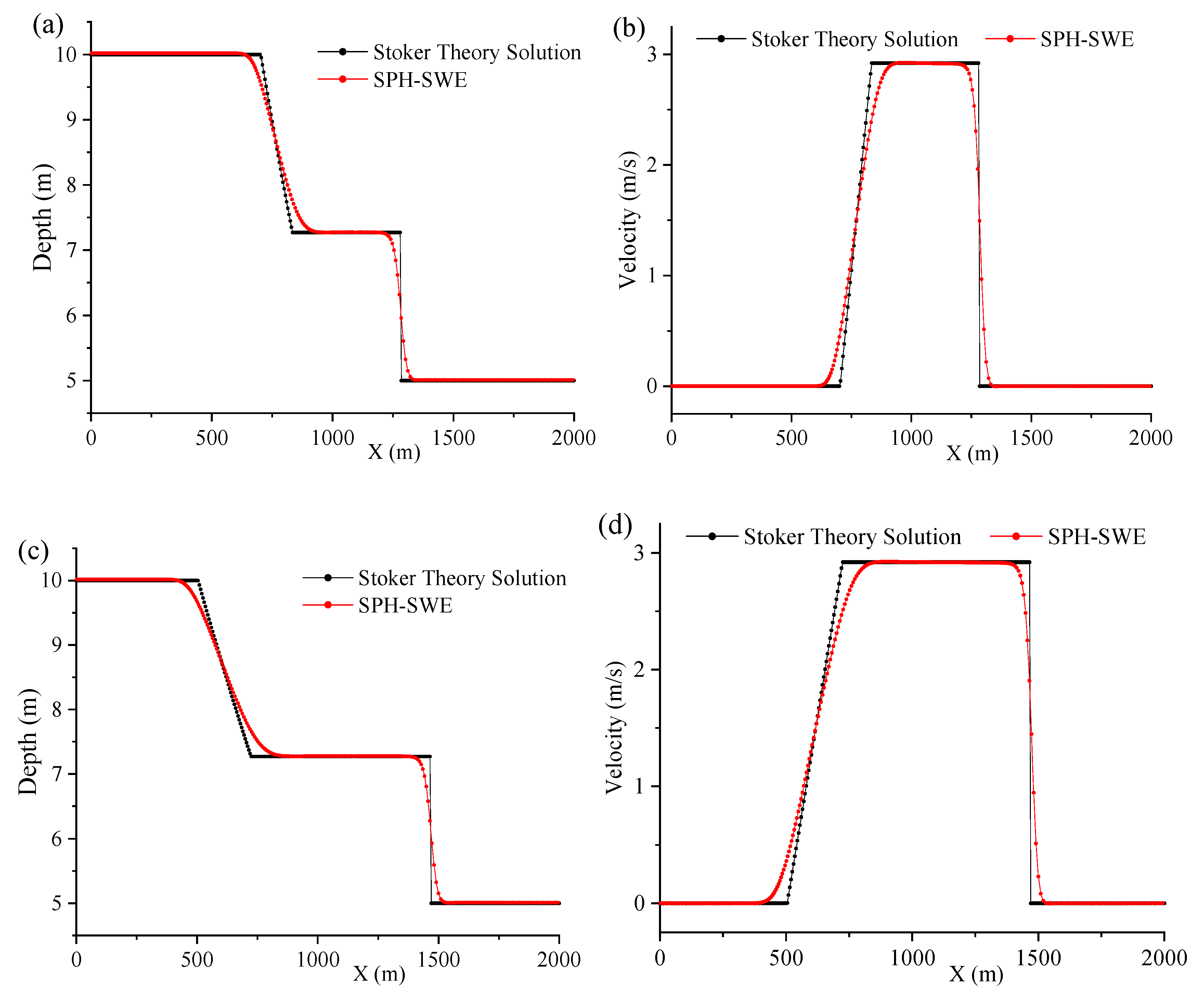
In order to verify the effect of the selected B-spline kernel function and the numerical oscillation processing method, a wet case was simulated (simulation range of 2000 m, initial water depth in the range of 0–1000 m is 10 m, and water depth in the range of 1000–2000 m is 5 m. The simulation time was 50 s, and the calculation results are generated every 10 s). The results are summarized in Table 2 and are shown in Figure 4.
According to the numbers displayed in Table 2, using the SPH-SWE model adopting the B-spline kernel function and the two-shocks Riemann solver method to solve the wet case, the simulation results are better, and their mean absolute errors to simulate velocity and water depth are within the 6%.
Based on these results, it was decided to select the B-spline kernel function and the two-shocks Riemann solver method to perform the two-dimensional dam-break numerical simulation to verify the computational efficiency of the new SPH-SWE model solution framework proposed.
3. SPH-SWE Model Solution Framework
When simulating dam break cases with a large number of particles involved, there is a challenge to be faced associated with low calculation efficiency. The code runs in serial steps and before each variable calculation, the mesh is divided into small grids (mesh size is 2H, smooth length, in order to calculate the corresponding parameters of each particle), making the process more repetitive and requiring a lot of calculation time. Moreover, the code framework is complex and it is demanding to complete any modification. As the open source code solves the model with a large number of particles, it has the problem of low calculation efficiency and cannot even be calculated (the reason is that the array overflows). This paper proposes a new SPH-SWE model solution framework, which can dynamically allocate the storage space of particle information, solve the problems of repeated particle search and unsuccessful memory allocation of the array of stored particle information, and can quickly solve the large-scale SPH-SWE model. Furthermore, the model framework proposed is simple, and any modification can be made easily to this algorithm.
For this study, Algorithm 1 was developed to solve the problem of data analysis and realize the CPU-OpenMP parallel computing.
| Algorithm 1. Calculation framework of the SPH-SWEs model. This algorithm is needed to read the particles data (include fluid particles/virtual particles/open boundary particle/riverbed particles). |
| Read parameters Output initial data of the model Mesh riverbed particles and calculate fluid particles and the net water depth Search particles dototal_number_of_timesteps
|
The calculation of each time step includes five parts, which can be summarized as follows:
- Calculation of fluid particles in the riverbed;
- Particle search, and calculation of the water depth;
- Calculation of the fluid particle depth and velocity gradient;
- Acceleration and riverbed gradient correction;
- Calculation of velocity and displacement rate.
In this paper, multiple two-dimensional arrays were used to store the information of fluid particles, riverbed particles, virtual particles, and open boundary particles. When calculating the parameters related to the above five parts, each particle can be calculated separately, and there is no dependency between particles.
Therefore, the CPU-OpenMP parallel computing can be realized (since each cycle is for all fluid particles, the calculation amount is known, so the schedule in the cycle configuration is set to Static mode) and the SPH-SWE model with a large number of particles can also be calculated.
3.1. Fluid Particle Riverbed Calculation
When calculating the riverbed particles in each time step, considering that the bed range and the smooth length of the riverbed particles are the same and there is no relationship between them, the calculation of the riverbed fluid particles was carried as follows.
Firstly, the grid division was completed, then the calculation of the riverbed fluid particles was conducted. It was verified that the calculation efficiency has no advantage, and additional array was needed to store riverbed particle information and increase data reading time. Please see below Algorithm 2 for the calculation framework adopted to achieve this task.
| Algorithm 2. Computing fluid particle riverbed. |
| 1. Stage 1: , initialize to 0 |
| 2. !$OMP PARALLEL DO PRIVATE(private variable),& |
| 3. !$OMP& SHARED(shared variable), DEFAULT(none), SCHEDULE(static) |
| 4. do total_number_of_fluid particles |
| 5. if particle_i is valid then |
| 6. Calculate particles’ mesh locations based on the riverbed’s mesh |
| 7. ! is used to make shepard correction(CSPM) |
| 8. CALL PURE celij_hb |
| 9. endif |
| 10. enddo |
| 11. !$OMP END PARALEL DO |
Because the calculated variables were two arrays, h_t and sum_h_t, it was not difficult to realize OpenMP parallel, and multiple threads were set to calculate the riverbed fluid particles at the same time, following these formulae:
After the calculation, the CSPM [79] was corrected, as shown in the next formula:
3.2. Particle Search
In this paper, the particle search technique [80,81] was used as a separate module to prepare for the calculation of parameters such as water depth, acceleration, and velocity.
In the particle search, the mesh was firstly divided, and then the mesh area of each particle search was calculated; in order to ensure the symmetry of particle interaction, less than 2hi or 2hj was used as the judgment condition of i effective particles.
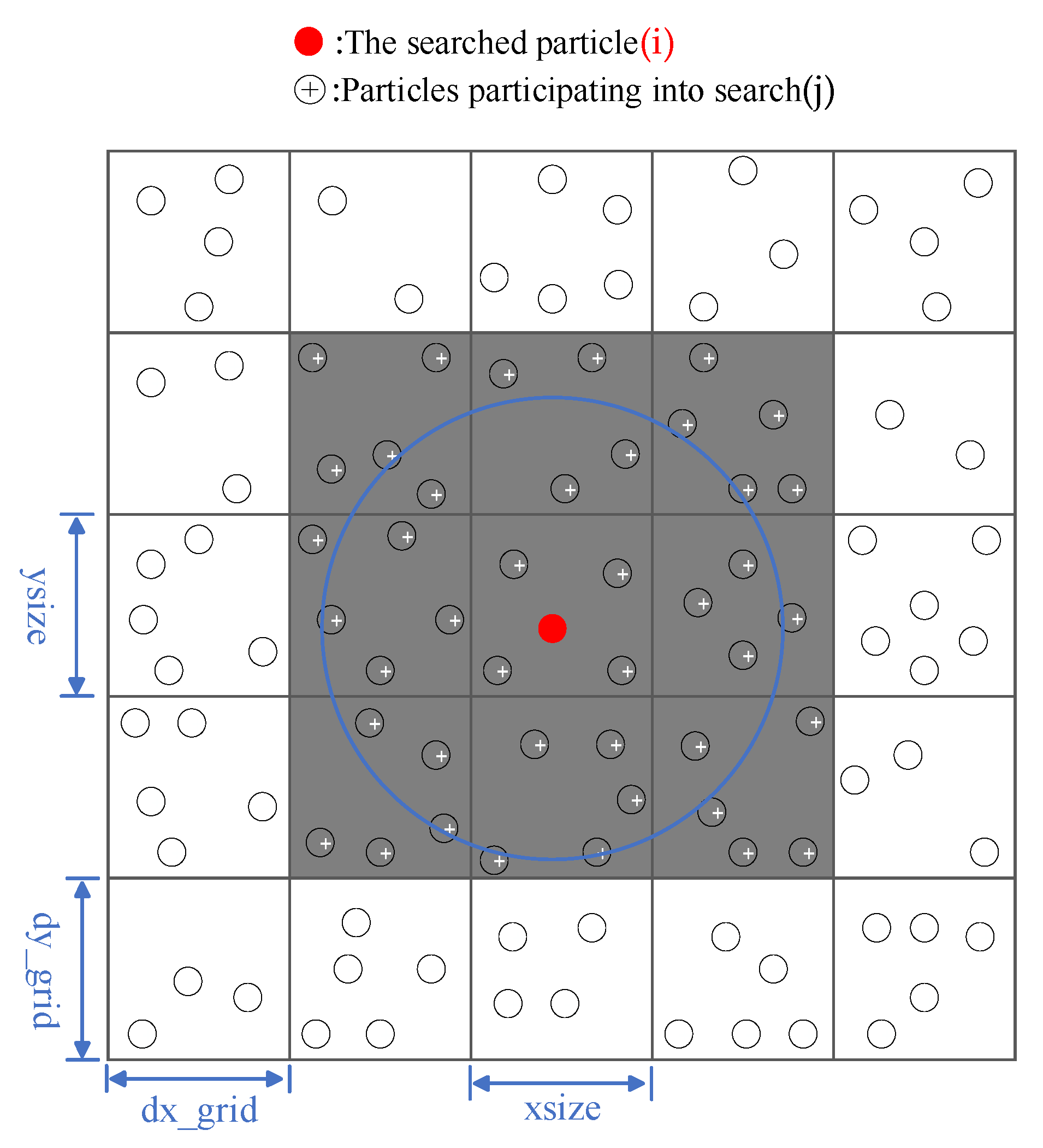
The specific steps of the particle search technique adopted [82] (see Figure 5) are described as follows:
- Before each time step, the temporary grid position was updated, and each grid was assigned to a unique number; the grid size can be set to a fixed size dx_grid/dy_grid;
- According to the position of the current SPH particles, all the SPH particles were allocated to the temporary mesh space, and the particle chain in the mesh was established;
- According to the range (2hi) of the tight support region of particle i, the search of other meshes (- xsize to xsize, - ysize to ysize) was completed in the tight support region of the mesh, storing the mesh number;
- All the SPH particles i and j in the mesh were searched (icell-xsize to icell + size, jcell-ysize to jcell + ysize) in the tight support domain.
To avoid high time consumption caused by repeated particle search in the meshless SPH-SWE model, Algorithm 3 was produced.
| Algorithm 3: The particle search. Read in the particles data (include fluid particles/virtual parti`cles/open boundary particle/riverbed particles). |
| 1. In each timestep 2. Mesh all particles based on fixed size dx_grid/dy_grid(generally select the maximum smooth length) and particles into nc array 3. ncx/ncy: total number of grids in x/y direction 4. iboxvv/iboxff/iboxob: store the virtual particles, fluid particles and open boundary particles within the affected region into two dimensional arrays 5. !$OMP PARALLEL DO PRIVATE (private variable),SHARED(shared variable),& 6. !$OMP& SHARED(shared variable),DEFAULT(none) 7. do total_number_of_fluid particles 8. if particle_i is valid then 9. Calculate mesh of the particle i:icell/jcell 10. Calculate search mesh range of particle i:xsize/yszie 11. do row -ysize,ysize 12. irow=jcell+1 13. do column -xsize,xsize 14. icolumn=icell+column 15. Calculate number of search grid: gridn 16. gridn=icolumn+(irow-1)*ncx 17. !Search for Virtual particles in the scope of I particle 18. do j nc(grindn,1) 19. if particle_i and particle_j are neighbours then 20. Write particle_j to iboxvv array 21. endif 22. enddo 23. !Search for Fluid particles in the scope of i particle 24. do j nc(grindn,2) 25. if particle_i and particle_j are neighbours then 26. Write particle_j to iboxff array 27. endif 28. enddo 29. !Search for Open boundary particles in the scope of i particle 30. do j nc(grindn,3) 31. if particle_i and particle_j are neighbours then 32. Write particle_j to iboxob array 33. endif 34. enddo 35. enddo 36. enddo 37. endif 38. enddo 39. !$OMP END PARALLEL DO |
In the open source code, the information of particles was stored in a three-dimensional array, and the grid was divided by a maximum smooth length of 2hmax (by adopting this, all particles can be stored into a cell, causing failure of memory allocation; however, the particle search method mentioned above solved this issue).
3.3. Water Depth Calculation
According to the Newton-iteration method, the water depth of particles was calculated, and the maximum number of iterations and the iteration-errors were taken as a criteria to terminate the iterations. In order to reduce the calculation time while ensuring the accuracy of the results, the maximum number of iterations of each particle was generally set to 50, and the iteration error was setup to 10−3. Nevertheless, different approaches can be selected according to different calculation models.
Before each calculation step, the water depth and smooth length of each particle were guessed. At the same time, the smooth length h and the correction coefficient αik were re-calculated and updated. In the same time step, the updated smooth length was then used for the sub-sequent SPH interpolation. The calculation framework is displayed in Algorithm 4.
| Algorithm 4: Water depth calculation. |
| 1. Stage 1: Guess for density and smoothed length 2. !$OMP PARALLEL DO PRIVATE(private variable),& 3. !$OMP& SHARED(shared variable),DEFAULT(none),SCHDULE(static) 4. do total_number_of_fluid particles 5. if particle_i is valid then 6. 1a: 7. 1b: 8. endif 9. enddo 10. !$OMP END PARALLEL DO 11. CALL particle search() %Search particles 12. Stage 2: Calculate depth 13. do while ((maxval(resmax) .gt. Minimum error) .and. (Iterationtimes .lt. max) 14. !$OMP PARALLEL DO PRIVATE(private variable),& 15. !$OMP& SHARED(shared variable),DEFAULT(none),SCHEDULE(static) 16. do total_number_of_fluid particles 17. if particle_i is valid then 18. CALL PURE fluid particle(i,rhop_sum(i),alphap(i)) 19. CALL PURE virtual particle(i,rhop_sum(i),alphap(i)) 20. CALL PURE open boundary particle((i,rhop_sum(i),alphap(i)) 21. %Calculate next step’s water depth and the smooth length 22. 23. 24. 25. 26. endif 27. enddo 28. !$OMP END PARALLEL DO 29. enddo |
After each water depth calculation, each particle was judged on whether the error requirements were met, and re-calculation was then completed for the particles that did not meet them. After this iteration cycle, the water depth, speed of the water, and volume were constantly updated.
3.4. Velocity Calculations
In order to calculate the acceleration () caused by internal force, the gradient of velocity and water depth had to be calculated, and the kernel function was adopted to complete this task as shown below:
where pi is the depth/velocity of particle i. The calculation conducted for this step is displayed in Algorithm 5.
| Algorithm 5: Calculation of fluid particle velocity and water depth gradient. |
| 1. Stage 1: sum_f/alphap/grad_up/grad_vp/grad_dw=0, Initialize to 0 2. !$OMP PARALLEL DO PRIVATE(private variable),& 3. !$OMP& SHARED(shared variable),DEFAULT(none),SCHDULE(static) 4. do total_number_of_fluid particles 5. if particle_i is valid then 6. !First conduct matrix for gradient correction 7. CALL PURE celij_corr(i,sum_f (I,1:4)) 8. CALL PURE celij_alpha(i,alphap(i),grad_dw(i,1:2),grad_up(i,1:2), grad_vp(i,1:2)) 9. CALL PURE celij_alpha_vir(i,alphap(i)) 10. CALL PURE celij_alphap_ob(i,alphap(i),grad_dw(i,1:2),grad_up(i,1:2), grad_vp(i,1:2)) 11. endif 12. enddo 13. !$OMP END PARALLEL DO |
If a variable time-step was implemented, the next step was to calculate the time-step according to Equation (9). The calculation framework of the time step included a loop and no sub-routine. It was found that the speed-up of time step parallel computing was less than 2 to perform serially variable time step calculations.
3.5. Calculation of Fluid Particle Acceleration, Riverbed Scouring, Speed, and Displacement
The acceleration () caused by the internal force was firstly calculated, followed by the riverbed gradient and the total acceleration (). After these calculations, the velocity and the displacement of fluid particles needed to be regularly updated as shown in the calculation framework Algorithm 6.
| Algorithm 6: Calculation of acceleration, velocity, and position. The Lagrangian equation of motion for a particle i is d/dt ∂L/(∂v_i )-∂L/(∂x_i )=0, where the Lagrangian functional L is defined in term of kinetic energy K and potential energy π as L = K-π, where π is a function of particles position but not velocity. |
| 1. Stage 1: Calculate 2. !$OMP PARALLEL DO PRIVATE(private variable),& 3. !$OMP& SHARED(shared variable),DEFAULT(none),SCHDULE(static) 4. do total_number_of_fluid particles 5. if particle_i is valid then 6. 1a. use Riemann solution to calculate 7. 1b. use Numerical viscosity to calculate 8. ! ar(i) is used to calculate depth 9. CALL PURE fluid particle(i,ar(i),ay(i),ar(i)) 10. CALL PURE virtual particle(i,ar(i),ay(i),ar(i)) 11. CALL PURE open boundary particle(i,ar(i),ay(i),ar(i)) 12. endif 13. Stage 2: Calculate 14. Stage 3: Calculate 15. Stage 4: Calculate velocity and position of fluid particle 16. enddo 17. !$OMP END PARALLEL DO |
If the open boundary was adopted, the displacement was updated, and it was checked whether it became a fluid particle or a buffer zone; if the case under investigation had a particle splitting zone, the fluid particles that meet the conditions identified were split [37]. Achieved this landmark, the calculation process was then completely repeated according to Algorithm 1.
4. Applications
4.1. Validation 1: 2-D Dry Bed Dam Break with Particle Splitting
In order to test the performance of the new computing SPH-SWE framework according to the CPU-OpenMP parallel computing, the open source case “2-D dry bed dam break with particle splitting”, referred to as DBDB case [67,68], was considered. Initial conditions of this open source DBDB case were setup as follows: area of 2.6 m × 1.2 m, initial fluid particle layout of 0.8 m × 1.2 m, and initial water depth equal to 0.15 m, as shown in Figure 6.
The spacing of the fluid particles was 0.015 m × 0.015 m, 0.01 m × 0.01 m, and 0.005 m × 0.005 m, respectively. Table 3 shows the number of fluid particles, virtual particles, and riverbed particles selected for the 3 cases tested (considering that no inflow and outflow conditions were set, the number of open boundary particles was maintained equal to 0).
The particles arrangements in the three cases were calculated using the open source code [67,68] and the CPU-OpenMP parallel code (in terms of 1000 particles per thread and 2000 particles per thread) to ensure that the calculation results were consistent and comparison of each model’s performance could be completed.
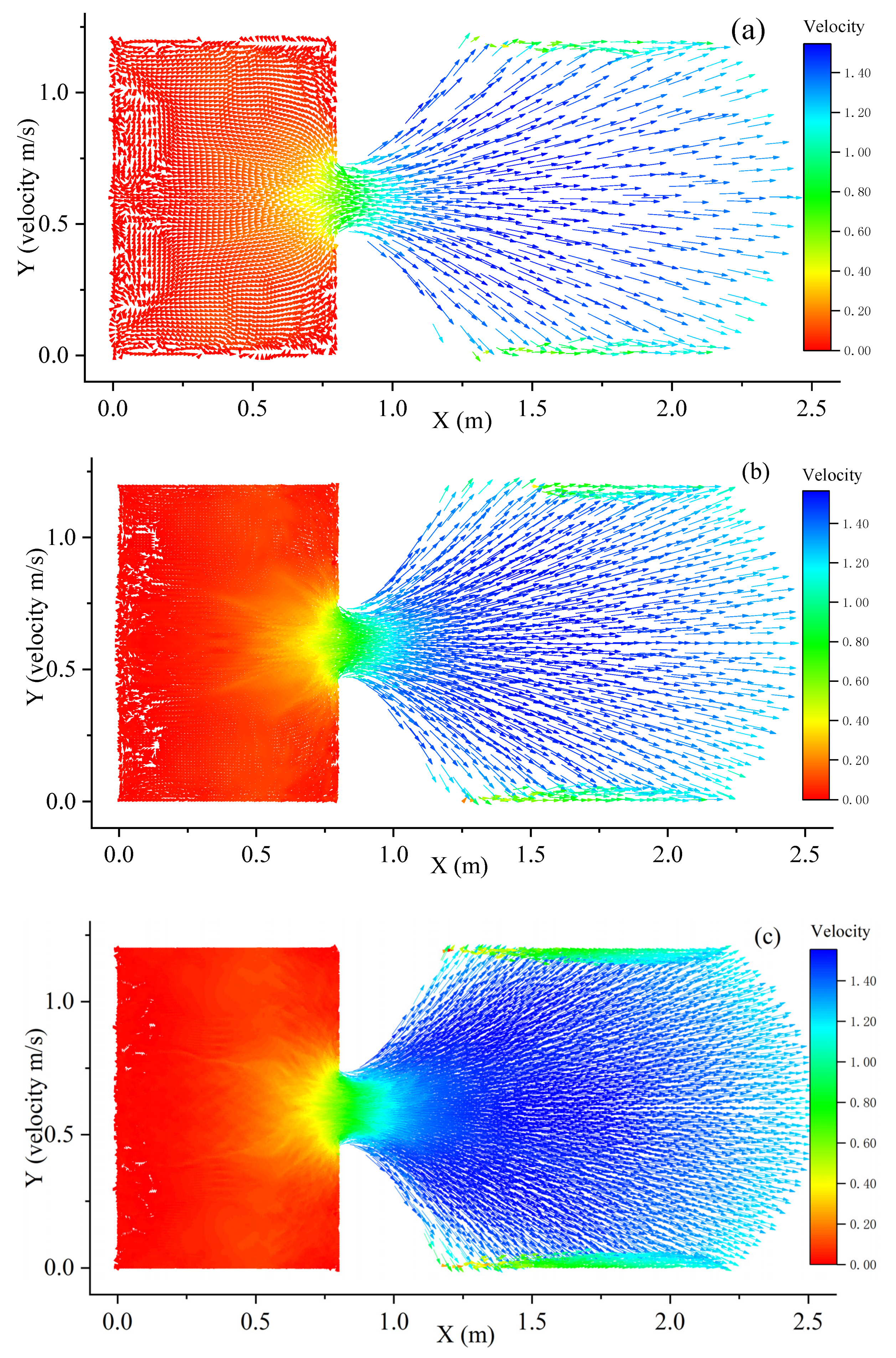
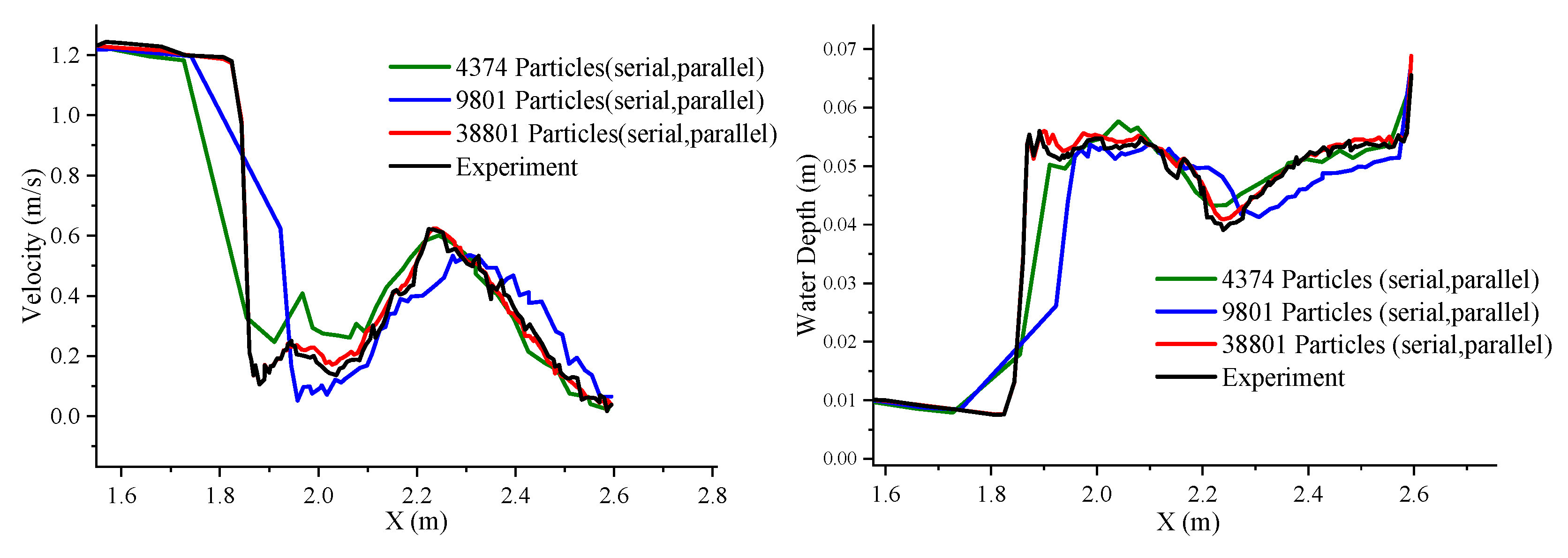
For t = 0, the instantaneous burst occurs and the fluid flows downstream. Figure 7 shows flow velocities for T = 1.2 s under the three fluid particle arrangements displayed in Table 3. It can be seen from Figure 7 that the more fluid particles there were, the more water flow characteristics and velocity distribution characteristics after dam break were seen. Figure 8 shows the comparison between numerical and experimental results for the three cases tested in Table 3.
It can be concluded that with the increase of fluid particles (Case 3), the error between the numerical and the experimental results was smaller.
Hence, bigger is the number of fluid particles computed, and more valuable are the water depth and velocity calculations for each time step and location across the dam system, therefore providing more support for the formulation of dam break mitigation plans. This also reflects the superiority of SPH-SWE model in dealing with large deformation and free surface problems.
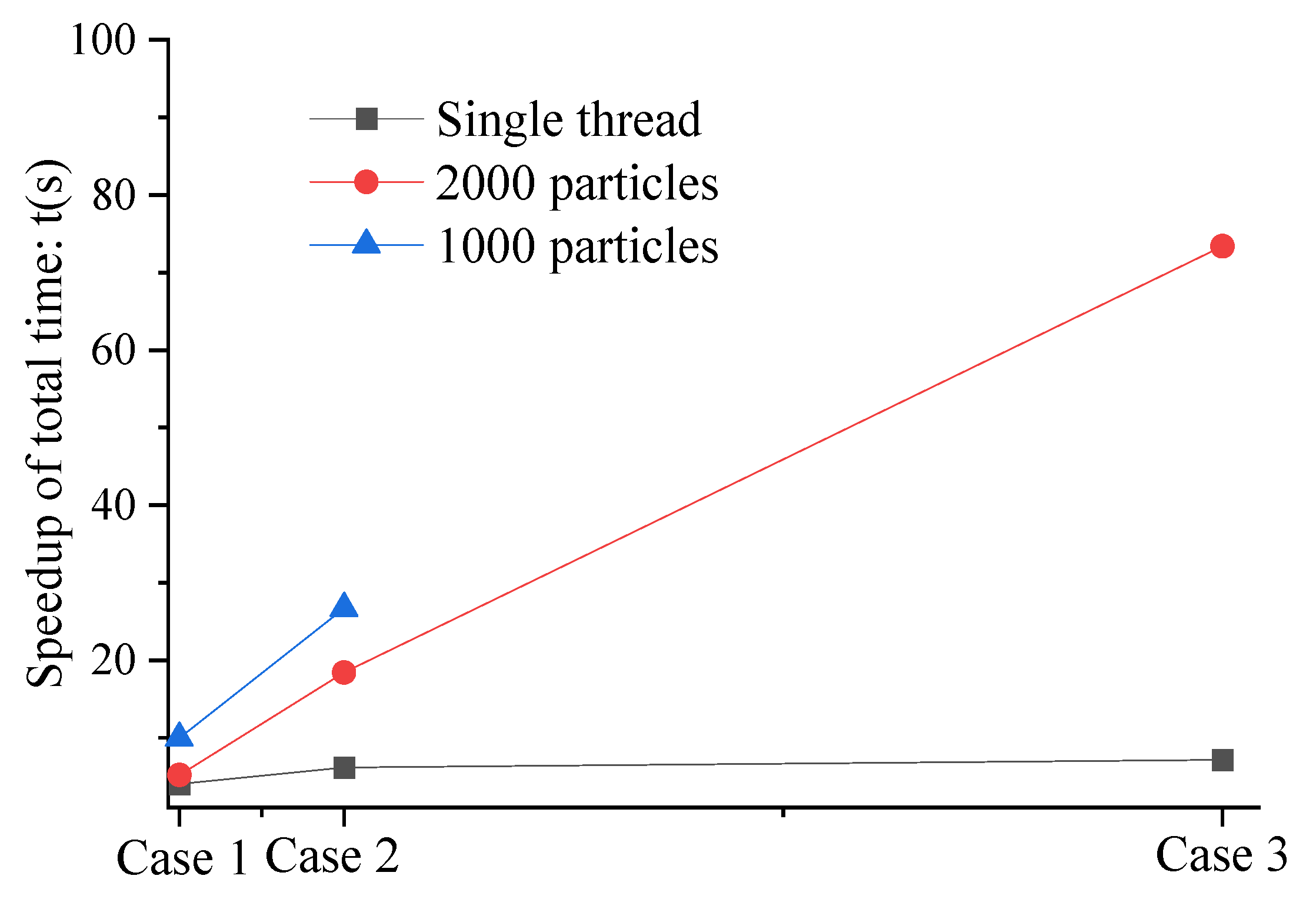
The time and speedup of total time t(s) (Equation (14)) required for calculating water depth, acceleration, speed, and displacement were quantified according to open source code and CPU-OpenMP parallel code (under different thread configurations) as shown in Table 4.
where t(k) represents the running time of open source code and t(c) represents the running time of the parallel code. In Table 4, R(t) represents the particle search time; C(t) represents the time to calculate the water depth; A(t) represents the time to calculate the acceleration, speed, and displacement; T(t) represents the total running time of the case (including t(k) and t(c)); the time unit is always seconds (s). It can be seen from the results that the number of particles computed was higher, and the parallel calculation was larger, based on CPU-OpenMP (Figure 9).
CPU-OpenMP allocated a thread according to 1000 fluid particles in parallel and calculated case 2 and case 3, in 26.7 s and 91.36 s, respectively.
In parallel computing, S(p) (the speedup ratio) and E(p) (parallel efficiency) were important indexes to evaluate the parallel effect. S(p) was the ratio between the serial time and the multi-core parallel time when threads calculate (p) and solved the iteration at the same time, as follows:
where, Ts is the time spent by a single processor in the serial mode; Tp is the time spent by threads (p) in the parallel mode. E(p) (parallel efficiency) is the ratio of the acceleration ratio to the number of CPU cores used in the calculation (and E(p) 1), indicating the average execution efficiency of each processor. When the acceleration ratio was close to the number of cores, the parallel efficiency was higher, and the utilization rate of each thread was higher, as calculated below.
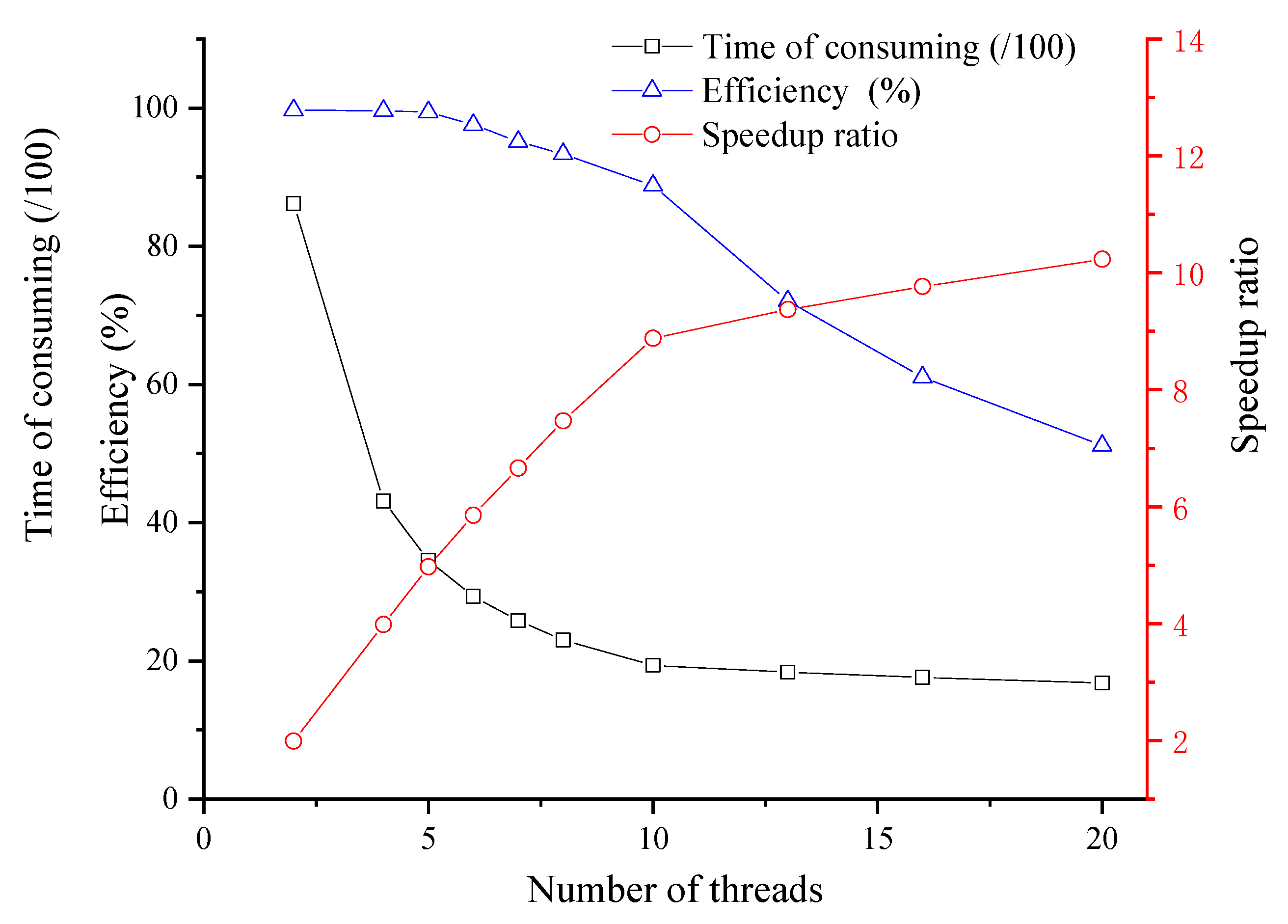
In order to check the parallel effect of CPU-OpenMP, case 3 was calculated with different threads. The acceleration ratio and parallel efficiency of different threads are shown in Table 5, and the performances of parallel algorithms are displayed in Figure 10.
According to Table 5 and Figure 10, as the number of enabled threads increased, the speedup ratio, parallel efficiency and calculation time were affected by the following trends: (1) the calculation time decreases with the increase of threads, but when the number of online processes exceeded 10, the time-consuming reduction speed changed from fast to slow reaching towards a balance; (2) the acceleration ratio increased all the time, but the improvements varied, and after 10 threads, the increase rate was from fast to slow; (3) the parallel efficiency decreased with the increase of threads, but the decrease rate fluctuated. When calculating the number of 10 threads, the parallel efficiency started to be less than 90%; therefore, case 3 could allocate one thread according to 5000 particles, with the acceleration ratio of 7.47 and the parallel efficiency of 93.35%.
4.2. Validation 2: 2-D Dam Break with A Rectangular Obstacle Located in the Downstream Area
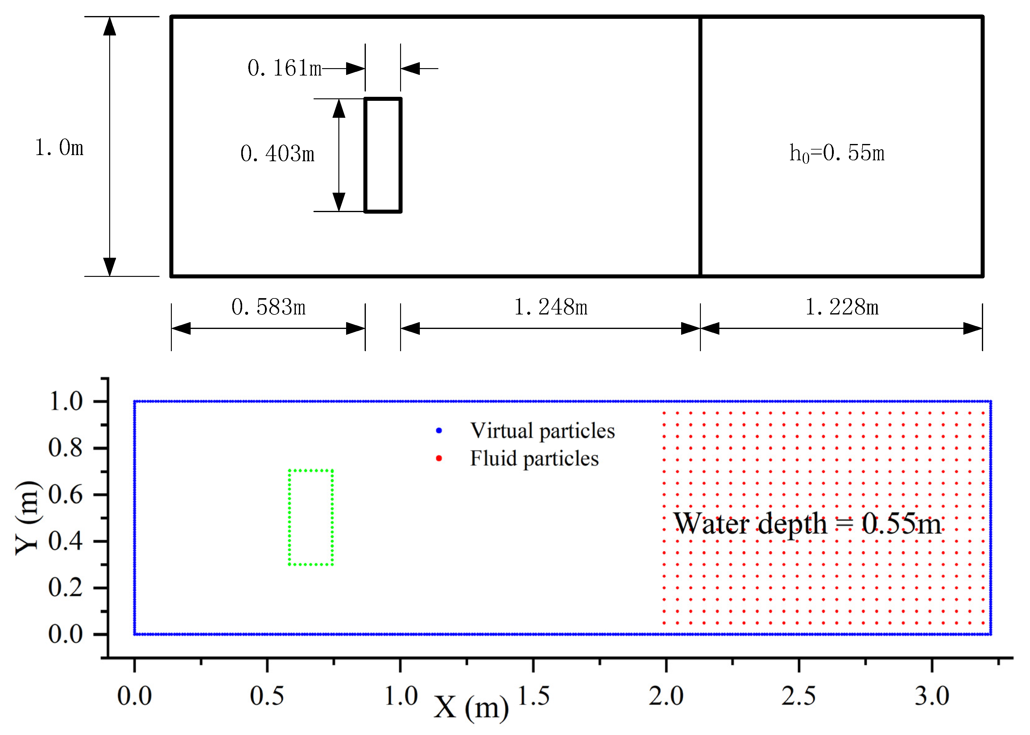
In order to solidify the accuracy and advantages of the new SPH-SWE model proposed calculated by CPU-OpenMP, a second case has been considered for validation. This case involved the dam break flow with a rectangular obstacle located in the downstream area as shown in Figure 11 [2,3,4,5,6,7,8,9,10,11,12,13,14,15,16,17,18,19,20,21,22,23,24,25,26,27,28,29,30,31,32,33,34,35,36,37,38,39,40,41,42,43,44,45,46,47,48,49,50,51,52,53,54,55,56,57,58,59,60,61,62,63,64,65,66,67,68,69,70,71,72,73,74,75,76,77,78,79,80,81,82,83].
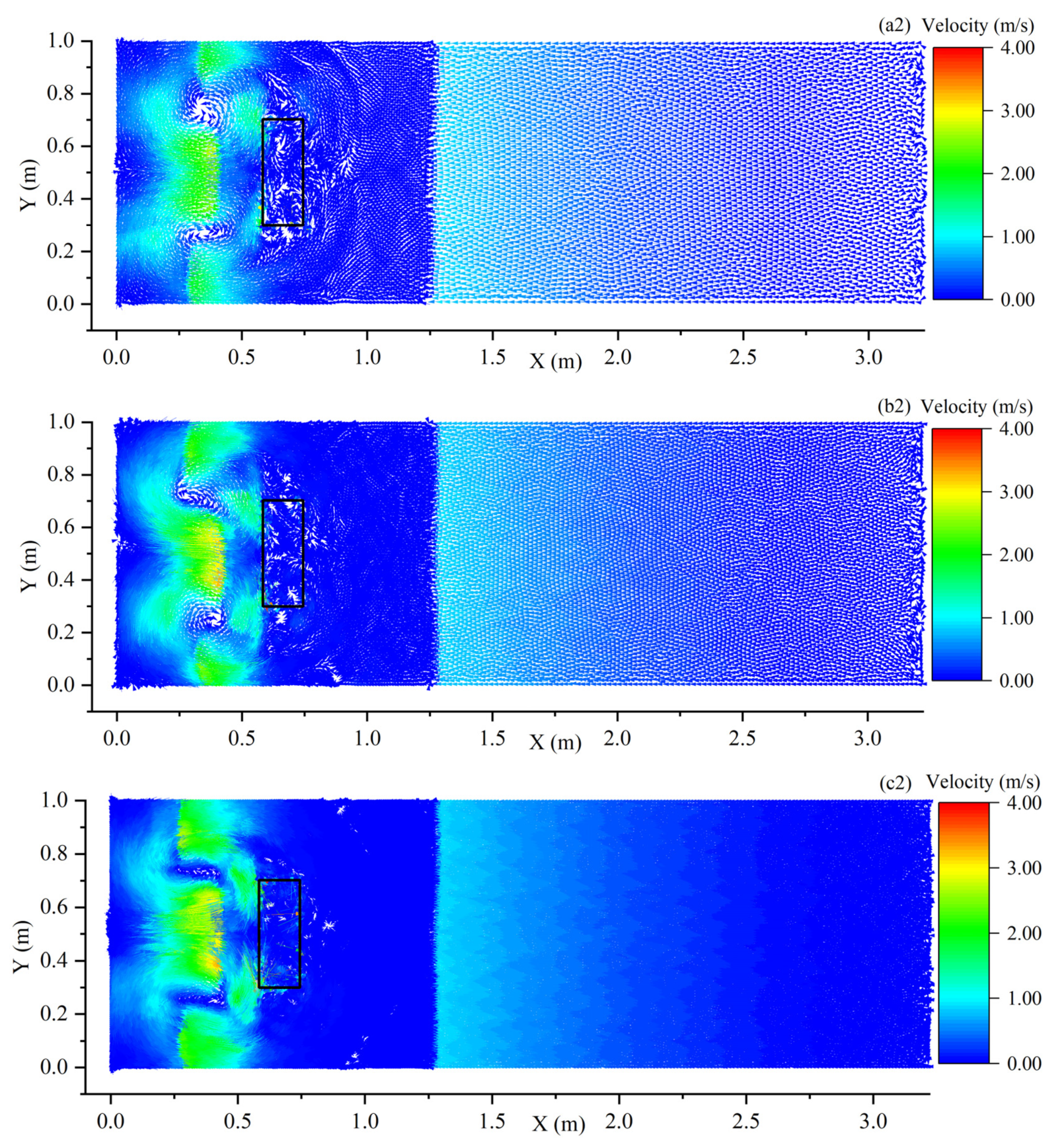
For this second validation scheme, the fluid particles were arranged according to the particle spacing of 0.01, 0.005, and 0.002 m. Figure 12 and Figure 13 display the results for t = 0.74 s and t = 1.76 s. for the same particle spacing used by Gu et al., [2] (0.01 m) and increasing number of fluid particles involved.
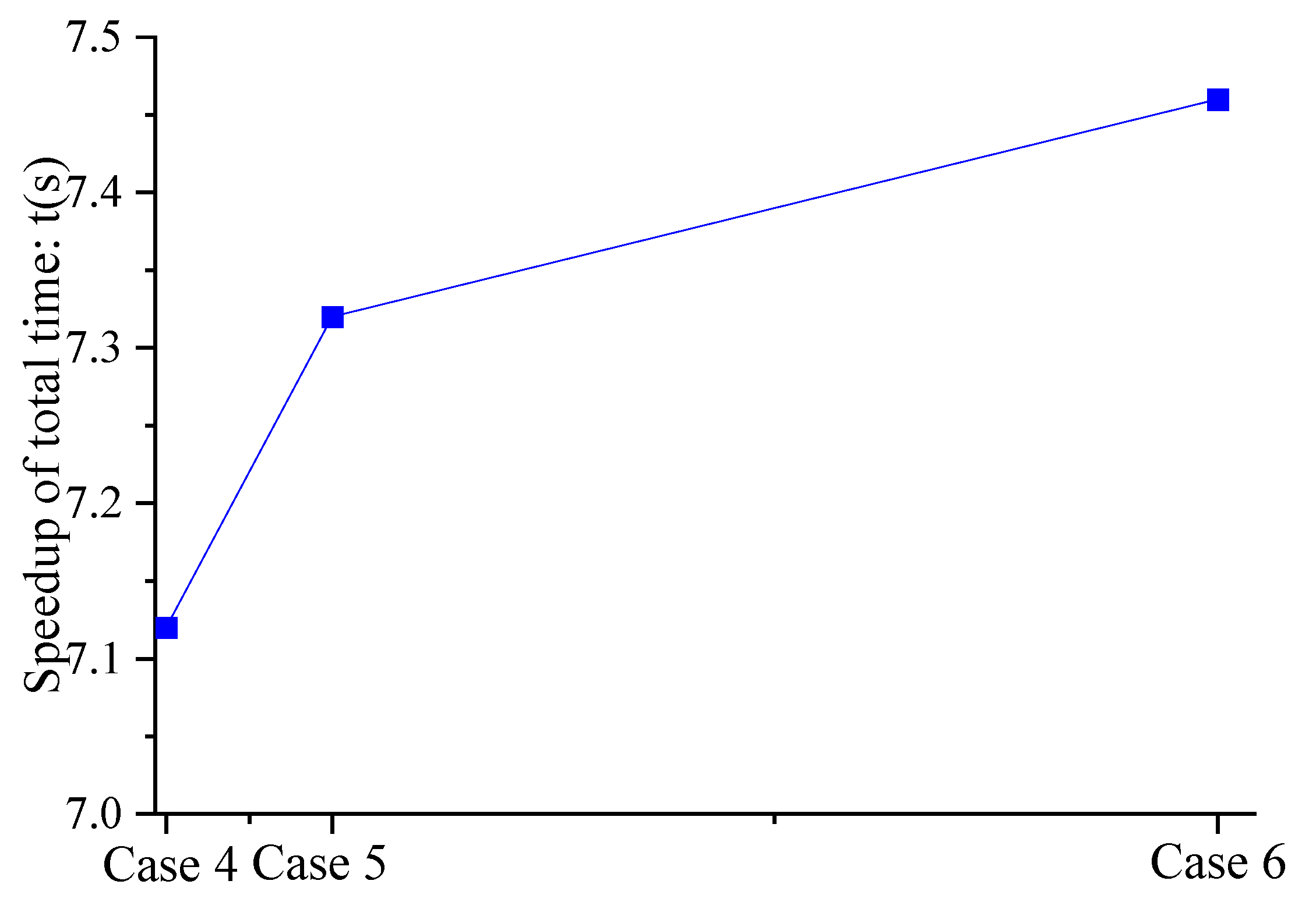
In Table 6, it is possible to check the number of particles involved in each simulation, and it can be noticed that the speed up of total time (t) slightly increased with the rise of particles (using 8 threads in all three processes) (Figure 14).
Table 7 unveils values of R(t), which represents the particle search time; C(t), which represents the time to calculate the water depth; and A(t), which represents the time to calculate the acceleration, speed, and displacement. It can be seen from the results (Figure 14) that when the number of particles computed was higher, the parallel calculation was slightly larger, based on CPU-OpenMP.
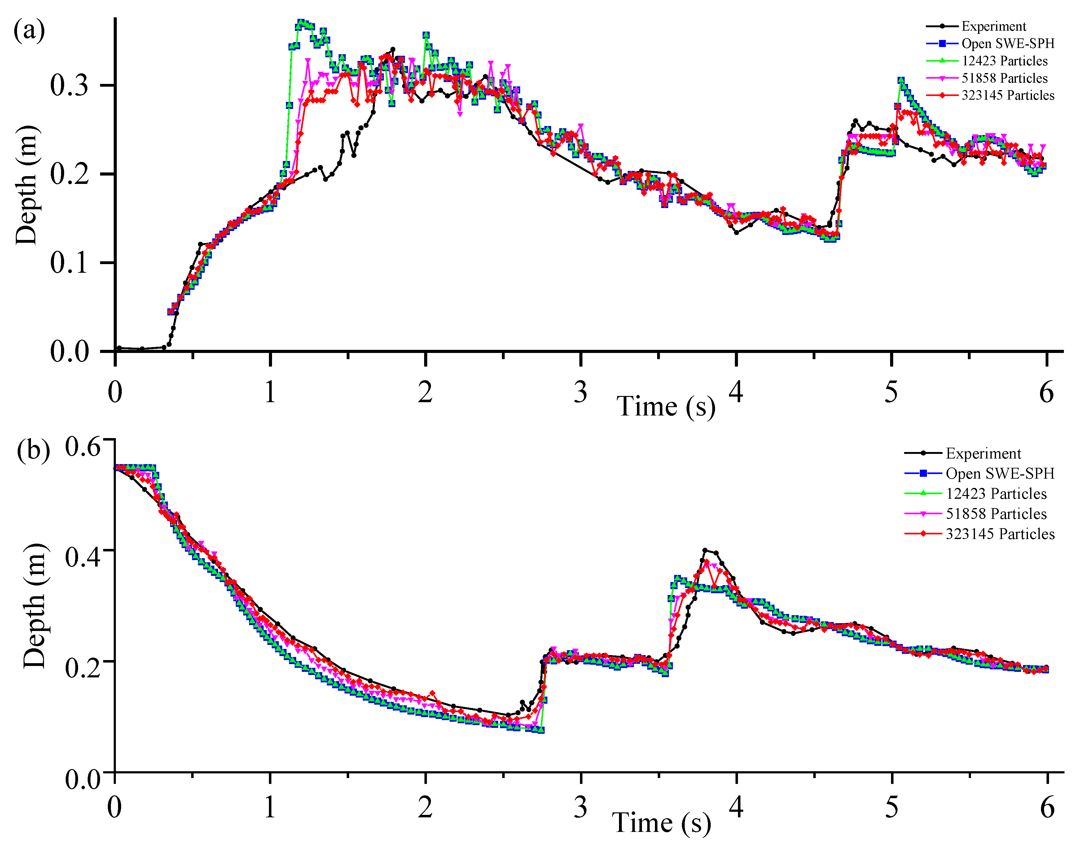
The simulation results are consistent with the previous case to demonstrate the improvement made by the proposed SPH-SWE calculation framework. When analyzing the same parameters as in the paper by Gu et al., [2], 12,423 fluid particles were involved. Results displayed in Figure 15 confirmed that the agreement between numerical results and experimental datasets improved even when simulating an increase of the number of fluid particles. However, the improvements do not involve the entire domain because in some positions (for example (a) H4 gauge, x = 1.3 m–1.8 m; (b) H2 gauge, x = 3.50 m–4.5 m) there are still minor inaccuracies (caused by the truncation error of the kernel function and the processing of boundary particles in the SPH method), even with the model with 323,145 fluid particles; hence, future work will focus on improving the algorithm to progress the calculation accuracy.
5. Conclusions
Vacondio et al. [34,35,36,37] made an open source version called SWE-SPHysics, which has been optimized and adapted based on the hydrodynamics investigated by other researchers during the last decade [38,39,40,41,42,43,44,45,46,47]. However, despite continuous progress, there was still a limitation related to the computational efficiency when the number of particles to simulate is very large, and this aspect still needs to be improved.
To fill this gap, in this study, a new solution to the SPH-SWE model introduced by Vacondio et al. [34,35,36,37] was proposed, and it was validated against two open source case studies of a 2-D dry-bed dam break with particle splitting [67,68] and of a 2-D dam break with a rectangular obstacle downstream [2,83]. To test the computing performance against the first case study, when involving large numbers of particles, three cases, involving different particles numbers, were tested (case 1—4374 particles; case 2—9801 particles; case 3—38,801 particles). Furthermore, this paper adopted the parallel computing method of CPU-OpenMP that is applied to a single machine and a multi-core to calculate the new SPH-SWEs framework.
By applying this CPU-OpenMP method, results have confirmed that the computing speeds of case 1/case 2/case 3 were increased by 4.01 times/6.14 times/7.17 times, respectively, to compute the new solution framework of the SPH-SWE model proposed to the open source case study previously mentioned [67,68]. According to the new solution framework of SPH-SWE model, case 3, characterized by the highest number of particles, was also calculated by using different threads. It was found that the speedup ratio can reach 7.47 when the parallel efficiency was more than 90%, which fully proves the good calculation performance of the CPU- OpenMP parallel new SPH-SWE model. Additionally, in the new solution framework of the SPH-SWE model proposed, particle search was used as a separate module for parallel computing, which greatly improved the computing efficiency and could replace the meshless SPH-SWE model in the open source code [67,68].
Therefore, using CPU-OpenMP parallel computing demonstrated that the SPH-SWE model new framework can accurately and timely simulate the flood evolution after a dam break.
In future works, the SPH-SWE model can be put into existing clusters to achieve more threads and further improve the calculation efficiency. Furthermore, this would enable the possibility of introducing more effective new algorithms into the SPH-SWE model (i.e., debris flow or water pollution modules) in order to expand its application. Continuous development of technology aids the improvement of new tools to design and inspect more accurate solutions, and this is an area in continuous development that needs to be addressed to support local and national authorities in making decisions to mitigate drastic effects generated by dam break.
Author Contributions
All authors contributed to the work. Conceptualization, S.G. and L.T.; methodology Y.W., M.R. and T.Y.; validation, Q.Z.; formal analysis, S.G., Y.W., M.R. and Z.X.; investigation, L.T., S.G., and M.R.; resources, S.G.; data curation, L.T. and M.R.; writing—review and editing, P.C., X.W., and M.R.; visualization, Q.Z.; supervision, S.G., M.R.; project administration, S.G.; funding acquisition, S.G. All authors have read and agreed to the published version of the manuscript.
Funding
This work was supported by the following projects: National Key R&D Program of China (No. 2017YFC0404303), National Natural Science Foundation of China (No.51869025, 51769028, 51868066), Qinghai Science and Technology Projects (No.2018-ZJ-710), Youth Fund of Qinghai University (Grant No. 2017-QGY-7), National Key Laboratory Project for Water Sand Science and Water and Hydropower Engineering, Tsinghua University (Grant No. sklhse-2018-B-03), Beijing Institute of Structure and Environment Engineering Fund(Grant No. BQ2019001).
Conflicts of Interest
The authors declare no conflict of interest.
References
- Chang, Y.S.; Chang, T.J. SPH simulations of solute transport in flows with steep velocity and concentration gradients. Water 2017, 9, 132. [Google Scholar] [CrossRef]
- Gu, S.; Zheng, X.; Ren, L.; Xie, H.; Huang, Y.; Wei, J.; Shao, S. SWE-SPHysics simulation of dam break flows at South-Gate Gorges Reservoir. Water 2017, 9, 387. [Google Scholar] [CrossRef] [Green Version]
- Chen, R.; Shao, S.; Liu, X.; Zhou, X. Applications of shallow water SPH model in mountainous rivers. J. Appl. Fluid Mech. 2015, 8, 863–870. [Google Scholar] [CrossRef]
- Peng, X.; Yu, P.; Chen, G.; Xia, M.; Zhang, Y. Development of a Coupled DDA–SPH Method and its Application to Dynamic Simulation of Landslides Involving Solid–Fluid Interaction. Rock Mech. Rock Eng. 2020, 53, 113–131. [Google Scholar] [CrossRef]
- Verbrugghe, T.; Dominguez, J.M.; Altomare, C.; Tafuni, A.; Vacondio, R.; Troch, P.; Kirtenhaus, A. Non-linear wave generation and absorption using open boundaries within DualSPHysics. Comput. Phys. Commun. 2019, 240, 46–59. [Google Scholar] [CrossRef]
- Ni, X.; Feng, W.; Huang, S.; Zhao, X.; Li, X. Hybrid SW-NS SPH models using open boundary conditions for simulation of free-surface flows. Ocean Eng. 2020, 196, 106845. [Google Scholar] [CrossRef]
- Gonzalez-Cao, J.; Altomare, C.; Crespo, A.J.C.; Dominguez, J.M.; Gomez-Gesteira, M.; Kisacik, D. On the accuracy of DualSPHysics to assess violent collisions with coastal structures. Comput. Fluids 2019, 179, 604–612. [Google Scholar] [CrossRef]
- Atif, M.M.; Chi, S.W.; Grossi, E.; Shabana, A. Evaluation of breaking wave effects in liquid sloshing problems: ANCF/SPH comparative study. Nonlinear Dyn. 2019, 97, 45–62. [Google Scholar] [CrossRef]
- Meringolo, D.D.; Marrone, S.; Colagrossi, A.; Liu, Y. A dynamic δ-SPH model: How to get rid of diffusive parameter tuning. Comput. Fluids 2019, 179, 334–355. [Google Scholar] [CrossRef]
- Shu, A.; Wang, S.; Rubinato, M.; Wang, M.; Qin, J.; Zhu, F. Numerical Modeling of Debris Flows Induced by Dam-Break Using the Smoothed Particle Hydrodynamics (SPH) Method. Appl. Sci. 2020, 10, 2954. [Google Scholar] [CrossRef]
- Wu, S.; Rubinato, M.; Gui, Q. SPH Simulation of interior and exterior flow field characteristics of porous media. Water 2020, 12, 918. [Google Scholar] [CrossRef] [Green Version]
- Wang, S.; Shu, A.; Rubinato, M.; Wang, M.; Qin, J. Numerical Simulation of Non-Homogeneous Viscous Debris-Flows based on the Smoothed Particle Hydrodynamics (SPH) Method. Water 2019, 11, 2314. [Google Scholar] [CrossRef] [Green Version]
- Gingold, R.A.; Monaghan, J.J. Smoothed particle hydrodynamics: Theory and application to non-spherical stars. Mon. Not. R. Astron. Soc. 1977, 181, 375–389. [Google Scholar] [CrossRef]
- Hopkins, P. A general class of Lagrangian smoothed particle hydrodynamics methods and implications for fluid mixing problems. Mon. Not. R. Astron. Soc. 2013, 428, 2840–2856. [Google Scholar] [CrossRef]
- Cremonesi, M.; Meduri, S.; Perego, U. Lagrangian-Eulerian enforcement of non-homogeneous boundary conditions in the Particle Finite Element Method. Comput. Part. Mech. 2020, 7, 41–56. [Google Scholar] [CrossRef]
- Sugiyama, K.; Li, S.; Takeuchi, S.; Takagi, S.; Matsumoto, Y. A full Eulerian finite difference approach for solving fluid-structure coupling problems. J. Comput. Phys. 2011, 230, 596–627. [Google Scholar] [CrossRef] [Green Version]
- Miller, G.H.; Colella, P. A conservative three-dimensional Eulerian method for coupled solid-fluid shock capturing. J. Comput. Phys. 2002, 183, 26–82. [Google Scholar] [CrossRef] [Green Version]
- Liu, M.B.; Liu, G.R. Smoothed Particle Hydrodynamics (SPH): An Overview and Recent Developments. Arch. Comput. Methods Eng. 2010, 17, 25–76. [Google Scholar] [CrossRef] [Green Version]
- Liu, G.R.; Liu, M.B. Smoothed Particle Hydrodynamics: A Meshfree Particle Method; World Scientific: Singapore, 2003. [Google Scholar]
- Dalrymple, R.A.; Rogers, B.D. Numerical modeling of water waves with the SPH method. Coast. Eng. 2006, 53, 141–147. [Google Scholar] [CrossRef]
- Huang, C.; Lei, J.M.; Peng, X.Y. A kernel gradient free (KGF) SPH method. Int. J. Numer. Methods Fluids 2015, 78. [Google Scholar] [CrossRef]
- Monaghan, J.J.; Kocharyan, A. SPH simulation of multi-phase flow. Comput. Phys. Commun. 1995, 87, 225–235. [Google Scholar] [CrossRef]
- Chen, A.S.; Djordjevic, S.; Leandro, J. An analysis of the combined consequences of pluvial and fluvial flooding. Water Sci. Technol. 2010, 62, 1491–1498. [Google Scholar] [CrossRef]
- Liang, Q.; Borthwick, A.G.L.; Stelling, G. Simulation of dam and dyke break hydrodynamics on dynamically adaptive quadtree grids. Int. J. Numer. Methods Fluids 2004, 46. [Google Scholar] [CrossRef]
- Chang, T.J.; Kao, H.M.; Chang, K.H.; Hsu, M.H. Numerical simulation of shallow water dam break flows in open channels using smoothed particle hydrodynamics. J. Hydrol. 2011, 408, 78–90. [Google Scholar] [CrossRef]
- Kao, H.M.; Chang, T.J. Numerical modeling of dambreak-induced flood inundation using smoothed particle hydrodynamics. J. Hydrol. 2012, 448–449, 232–244. [Google Scholar] [CrossRef]
- Colagrossi, A.; Landrini, M. Numerical simulation of interfacial flows by smoothed particle hydrodynamics. J. Comput. Phys. 2003, 191, 448–475. [Google Scholar] [CrossRef]
- Yang, F.L.; Zhang, X.F.; Tan, G.M. One and two-dimensional coupled hydrodynamics model for dam break flow. J. Hydrodyn. 2007, 19, 769–775. [Google Scholar] [CrossRef]
- Wang, Z.; Shen, H.T. Lagrangian simulation of one-dimensional dam-break flow. Hydraul. Eng. 1999, 125, 1217–1220. [Google Scholar] [CrossRef]
- Ata, R.; Soulaimani, A. A stabilized SPH method for inviscid shallow water flows. Int. J. Numer. Methods Fluids 2005, 47, 139–159. [Google Scholar] [CrossRef]
- Leffe, M.D.; Touzé, D.L.; Alessandrini, B. SPH Modeling of a shallow-water coastal flows. Hydraul. Res. 2010, 48, 118–125. [Google Scholar] [CrossRef]
- Rodriguez-Paz, M.; Bonet, J. A corrected smooth particle hydrodynamics formulation of the shallow-water equations. Comput. Struct. 2005, 83, 1396–1410. [Google Scholar] [CrossRef]
- Panizzo, A.; Longo, D.; Bellotti, G.; De Girolamo, P. Tsunamis early warning system. Part 3: SPH modeling of nlswe. In Proceedings of the XXX Convegno di Idraulica e Costruzioni Idrauliche, Rome, Italy, 10–15 September 2006. [Google Scholar]
- Vacondio, R.; Rogers, B.D.; Stansby, P.K.; Mignosa, P. A correction for balancing discontinuous bed slopes in two-dimensional smoothed particle hydrodynamics shallow water modeling. Int. J. Numer. Methods Fluids 2013, 71, 850–872. [Google Scholar] [CrossRef]
- Vacondio, R.; Rogers, B.D.; Stansby, P.K.; Mignosa, P. SPH Modeling of Shallow Flow with Open Boundaries for Practical Flood Simulation. J. Hydraul. Eng. 2012, 138, 530–541. [Google Scholar] [CrossRef]
- Vacondio, R.; Rogers, B.D.; Stansby, P.K.; Mignosa, P. Smoothed Particle Hydrodynamics: Approximate zero-consistent 2-D boundary conditions and still shallow water tests. Int. J. Numer. Methods Fluids 2011, 69, 226–253. [Google Scholar] [CrossRef]
- Vacondio, R.; Rogers, B.D.; Stansby, P.K. Accurate particle splitting for SPH in shallow water with shock capturing. Int. J. Numer. Methods Fluids 2012, 69, 1377–1410. [Google Scholar] [CrossRef]
- Skillen, A.; Lind, S.J.; Stansby, P.K.; Rogers, B.D. Incompressible Smoothed Particle Hydrodynamics (SPH) with reduced temporal noise and generalised Fickian smoothing applied to body-water slam and efficient wave-body interaction. Comput. Methods Appl. Mech. Eng. 2013, 265, 163–173. [Google Scholar] [CrossRef]
- Fourtakas, G.; Rogers, B.D.; Laurence, D.R.P. Modelling Sediment resuspension in Industrial tanks using SPH. Houille Blanche 2013, 2, 39–45. [Google Scholar] [CrossRef]
- St-Germain, P.; Nistor, I.; Townsend, R.; Shibayama, T. Smoothed-Particle Hydrodynamics Numerical Modeling of Structures Impacted by Tsunami Bores. J. Waterw. Port Coast. Ocean Eng. 2014, 140, 66–81. [Google Scholar] [CrossRef]
- Cunningham, L.S.; Rogers, B.D.; Pringgana, G. Tsunami wave and structure interaction: An investigation with smoothed-particle hydrodynamics. Proc. Inst. Civ. Eng. Eng. Comput. Mech. 2014, 167, 106–116. [Google Scholar] [CrossRef] [Green Version]
- Aureli, F.; Dazzi, S.; Maranzoni, A.; Mignosa, P.; Vacondio, R. Experimental and numerical evaluation of the force due to the impact of a dam-break wave on a structure. Adv. Water Resour. 2015, 76, 29–42. [Google Scholar] [CrossRef]
- Canelas, R.B.; Domínguez, J.M.; Crespo, A.J.C.; Gómez-Gesteira, M.; Ferreira, R.M.L. A Smooth Particle Hydrodynamics discretization for the modelling of free surface flows and rigid body dynamics. Int. J. Numer. Methods Fluids 2015, 78, 581–593. [Google Scholar] [CrossRef]
- Heller, V.; Bruggemann, M.; Spinneken, J.; Rogers, B.D. Composite modelling of subaerial landslide–tsunamis in different water body geometries and novel insight into slide and wave kinematics. Coast. Eng. 2016, 109, 20–41. [Google Scholar] [CrossRef]
- Fourtakas, G.; Rogers, B.D. Modelling multi-phase liquid-sediment scour and resuspension induced by rapid flows using Smoothed Particle Hydrodynamics (SPH) accelerated with a graphics processing unit (GPU). Adv. Water Resour. 2016, 92, 186–199. [Google Scholar] [CrossRef]
- Mokos, A.; Rogers, B.D.; Stansby, P.K. A multi-phase particle shifting algorithm for SPH simulations of violent hydrodynamics with a large number of particles. J. Hydraul. Res. 2017, 55, 143–162. [Google Scholar] [CrossRef] [Green Version]
- Alshaer, A.W.; Rogers, B.D.; Li, L. Smoothed Particle Hydrodynamics (SPH) modelling of transient heat transfer in pulsed laser ablation of Al and associated free-surface problems. Comput. Mater. Sci. 2017, 127, 161–179. [Google Scholar] [CrossRef]
- Sun, P.N.; Colagrossi, A.; Marrone, S.; Antuono, M.; Zhang, A.M. A consistent approach to particle shifting in the δ-Plus-SPH model. Mech. Eng. 2019, 348, 912–934. [Google Scholar] [CrossRef]
- Sun, P.; Zhang, A.M.; Marrone, S.; Ming, F. An accurate and efficient SPH modeling of the water entry of circular cylinders. Appl. Ocean Res. 2018, 72, 60–75. [Google Scholar] [CrossRef]
- Zheng, X.; Shao, S.; Khayyer, A.; Duan, W.; Ma, Q.; Liao, K. Corrected first-order derivative ISPH in water wave simulations. Coast. Eng. J. 2017, 59. [Google Scholar] [CrossRef]
- Luo, M.; Reeve, D.; Shao, S.; Karunarathna, H.; Lin, P.; Cai, H. Consistent Particle Method simulation of solitary wave impinging on and overtopping a seawall. Eng. Anal. Bound. Elem. 2019, 103, 160–171. [Google Scholar] [CrossRef]
- Ran, Q.; Tong, J.; Shao, S.; Fu, X.; Xu, Y. Incompressible SPH scour model for movable bed dam break flows. Adv. Water Resour. 2015, 82, 39–50. [Google Scholar] [CrossRef] [Green Version]
- Xia, X.; Liang, Q. A GPU-accelerated smoothed particle hydrodynamics (SPH) model for the shallow water equations. Environ. Model. Softw. 2016, 75, 28–43. [Google Scholar] [CrossRef]
- Liang, Q.; Xia, X.; Hou, J. Catchment-scale High-resolution Flash Flood Simulation Using the GPU-based Technology. Procedia Eng. 2016, 154, 975–981. [Google Scholar] [CrossRef] [Green Version]
- Satake, S.I.; Yoshimori, H.; Suzuki, T. Optimazations of a GPU accelerated heat conduction equation by a programming of CUDA Fortran from an analysis of a PTX file. Comput. Phys. Commun. 2012, 183, 2376–2385. [Google Scholar] [CrossRef]
- Yang, C.T.; Huang, C.L.; Lin, C.F. Hybrid CUDA, OpenMP, and MPI parallel programming on multicore GPU clusters. Comput. Phys. Commun. 2011, 182, 266–269. [Google Scholar] [CrossRef]
- Ohshima, S.; Hirasawa, S.; Honda, H. OMPCUDA: OpenMP Execution Framework for CUDA Based on Omni OpenMP Compiler. In Beyond Loop Level Parallelism in OpenMP: Accelerators, Tasking and More; Sato, M., Hanawa, T., Müller, M.S., Chapman, B.M., de Supinski, B.R., Eds.; IWOMP 2010. Lecture Notes in Computer Science, 6132; Springer: Berlin/Heidelberg, Germany, 2010. [Google Scholar] [CrossRef]
- Loncar, V.; Young, S.L.E.; Skrbic, S.; Muruganandam, P.; Adhikari, S.; Balaz, A. OpenMP, OpenMP/MPI, and CUDA/MPI C programs for solving the time-dependent dipolar Gross-Pitaevskii equation. Comput. Phys. Commun. 2016, 209, 190–196. [Google Scholar] [CrossRef] [Green Version]
- Bronevetsky, G.; Marques, D.; Pingali, K.; McKee, S.; Rugina, R. Compiler-enhanced incremental checkpointing for OpenMP applications. In Proceedings of the 2009 IEEE International Symposium on Parallel & Distributed Processing, Rome, Italy, 23–29 May 2009; pp. 1–12. [Google Scholar] [CrossRef] [Green Version]
- Dagum, L.; Menon, R. OpenMP: An industry standard API for shared-memory programming. IEEE Comput. Sci. Eng. 1998, 5, 46–55. [Google Scholar] [CrossRef] [Green Version]
- Slabaugh, G.; Boyes, R.; Yang, X. Multicore Image Processing with OpenMP [Applications Corner]. IEEE Signal Process. Mag. 2010, 27, 134–138. [Google Scholar] [CrossRef]
- Chorley, M.J.; Walker, D.W. Performance analysis of a hybrid MPI/OpenMP application on multi-core clusters. J. Comput. Sci. 2010, 1, 168–174. [Google Scholar] [CrossRef] [Green Version]
- Adhianto, L.; Chapman, B. Performance modeling of communication and computation in hybrid MPI and OpenMP applications. Simul. Model. Pract. Theory 2007, 15, 481–491. [Google Scholar] [CrossRef]
- Wright, S.J. Parallel algorithms for banded linear systems. Siam J. Sci. Stat. Comput. 1991, 12, 824–842. [Google Scholar] [CrossRef]
- Jiao, Y.-Y.; Zhao, Q.; Wang, L. A hybrid MPI/OpenMP parallel computing model for spherical discontinuous deformation analysis. Comput. Geotech. 2019, 106, 217–227. [Google Scholar] [CrossRef]
- Przemysław, S. Algorithmic and language-based optimization of Marsa-LFIB4 pseudorandom number generator using OpenMP, OpenACC and CUDA. J. Parallel Distrib. Comput. 2020, 137, 238–245. [Google Scholar]
- Vacondio, R. Shallow Water and Navier-Stokes SPH-Like Numerical Modelling of Rapidly Varying Free-Surface Flows. Ph.D. Thesis, Università degli Studi di Parma, Parma, Italy, 2010. [Google Scholar]
- Vacondio, R.; Rodgers, B.D.; Stansby, P.K.; Mignosa, P. User Guide for the SWE-SPHysics Code. 2013. Available online: https://wiki.manchester.ac.uk/sphysics/images/SWE-SPHysics_v1.0.00.pdf (accessed on 2 April 2020).
- Marion, J.; Thornton, S. Classical Dynamics of Particles and Systems; Harcourt Brace Jovanovich Inc.: San Diego, CA, USA, 1988. [Google Scholar]
- Monaghan, J.J. Smoothed particle hydrodynamics. Rep. Prog. Phys. 2005, 68, 1703–1759. [Google Scholar] [CrossRef]
- Bonet, J.; Lok, T.-S.L. Variational and momentum preservation aspects of Smooth Particle Hydrodynamic formulations. Comput. Methods Appl. Mech. Eng. 1999, 180, 97–115. [Google Scholar] [CrossRef]
- Vila, J.P. On particle weighted methods and smooth particle hydrodynamics. Math. Models Methods Appl. Sci. 1999, 9, 161–209. [Google Scholar] [CrossRef]
- Dinshaw, B.S. Von Neumann stability analysis of smoothed particle hydrodynamics—Suggestions for optimal algorithms. J. Comput. Phys. 1995, 121, 357–372. [Google Scholar]
- Toro, E. Direct Riemann solvers for the time-dependent Euler equations. Shock Waves 1995, 5, 75–80. [Google Scholar] [CrossRef]
- Hernquist, L.; Katz, N. TREESPH: A unification of SPH with the hierarchical tree method. Astrophys. J. Suppl. 1989, 70, 419–446. [Google Scholar] [CrossRef]
- Toro, E. Shock Capturing Methods for Free Surface Shallow Water Flows; Wiley: New York, NY, USA, 1999. [Google Scholar]
- Nikolaos, D.K. A dissipative galerkin scheme for open-channel flow. Hydraul. Eng. 1984, 110, 337–352. [Google Scholar]
- Majda, A.; Osher, S. Numerical viscosity and the entropy condition. Commun. Pure Appl. Math. 1979. [Google Scholar] [CrossRef]
- Stranex, T.; Wheaton, S. A new corrective scheme for SPH. Comput. Methods Appl. Mech. Eng. 2011, 200, 392–402. [Google Scholar] [CrossRef]
- Monaghan, J.J.; Gingold, R.A. Shock simulation by the particle method SPH. J. Comput. Phys. 1983, 52, 374–389. [Google Scholar] [CrossRef]
- Monaghan, J.J. Particle methods for hydrodynamics. Comput. Phys. Rep. 1985, 3, 71–124. [Google Scholar] [CrossRef]
- Chen, F.; Qiang, H.; Gao, W. Coupling of smoothed particle hydrodynamics and finite volume method for two-dimensional spouted beds. Comput. Chem. Eng. 2015, 77, 135–146. [Google Scholar] [CrossRef]
- Kleefsman, K.M.T.; Fekken, G.; Veldman, A.E.P.; Iwanowski, B.; Buchner, B. A volume-of-fluid based simulation method for wave impact problems. J. Comput. Phys. 2005, 206, 363–393. [Google Scholar] [CrossRef] [Green Version]
Figure 1.
Simulation results of different kernel functions. (a,c) Results of water depths calculations. (b,d) Results of velocity calculations.
Figure 1.
Simulation results of different kernel functions. (a,c) Results of water depths calculations. (b,d) Results of velocity calculations.

Figure 2.
Absolute errors of different kernel functions and processing methods. (a–c) The absolute errors of water depth and velocity calculated by B-spline kernel function, quartic spline, and quadratic spline kernel function, respectively. (d) The absolute errors of water depth and velocity calculated by using the artificial viscosity method.

Figure 3.
Simulation results of different processing methods.

Figure 4.
Simulation results of the SPH-SWE module. (a,b) water depth and velocity diagram at t = 30 s; (c,d) water depth and velocity diagram at t = 50 s.
Figure 4.
Simulation results of the SPH-SWE module. (a,b) water depth and velocity diagram at t = 30 s; (c,d) water depth and velocity diagram at t = 50 s.

Figure 5.
Framework of particle search [81].
Figure 5.
Framework of particle search [81].

Figure 6.
2-D dry bed dam break with particle splitting (DBDB) case setup.

Figure 7.
Results of 2-D Dry-Bed Dam Break with particle splitting at 1.2 s obtained from the simulations with: (a) 4374 particles; (b) 9801 particles; (c) 38,801 particles.
Figure 7.
Results of 2-D Dry-Bed Dam Break with particle splitting at 1.2 s obtained from the simulations with: (a) 4374 particles; (b) 9801 particles; (c) 38,801 particles.

Figure 8.
Numerical vs. experimental results comparison (velocities on the left and water depths on the right).
Figure 8.
Numerical vs. experimental results comparison (velocities on the left and water depths on the right).

Figure 9.
Speedup of total runtime for validation 1.

Figure 10.
CPU-OpenMP model parallel computing performances.

Figure 11.
Scheme of the second model used for validation of the new SPH-SWE model proposed [2,3,4,5,6,7,8,9,10,11,12,13,14,15,16,17,18,19,20,21,22,23,24,25,26,27,28,29,30,31,32,33,34,35,36,37,38,39,40,41,42,43,44,45,46,47,48,49,50,51,52,53,54,55,56,57,58,59,60,61,62,63,64,65,66,67,68,69,70,71,72,73,74,75,76,77,78,79,80,81,82,83].

Figure 12.
Velocity distribution at 0.74 s for Case 4 (a1), 5 (b1) and 6 (c1) displayed in Table 6.
Figure 12.
Velocity distribution at 0.74 s for Case 4 (a1), 5 (b1) and 6 (c1) displayed in Table 6.

Figure 13.
Velocity distribution at 1.76 s for Case 4 (a2), 5 (b2) and 6 (c2) displayed in Table 6.
Figure 13.
Velocity distribution at 1.76 s for Case 4 (a2), 5 (b2) and 6 (c2) displayed in Table 6.

Figure 14.
Speedup of total runtime for validation 2.

Figure 15.
Comparison between experimental and numerical results water depth datasets: (a) gauge H4 in [2] and [80]; (b) gauge H2 in [2] and [80].


Table 1.
Error analysis.
| Parameters | Artificial Viscosity | Lax Friedrichs Flux | Two-Shocks Riemann Solver | |
|---|---|---|---|---|
| Mean Absolute Error | Speed | 0.0617 | 0.0476 | 0.0351 |
| WD | 0.0515 | 0.0482 | 0.0356 | |
| Mean Relative Error | Speed | 0.0718 | 0.0667 | 0.0586 |
| WD | 0.0142 | 0.0089 | 0.0092 | |
| Standard deviation of error | Speed | 0.1042 | 0.0728 | 0.0568 |
| WD | 0.0681 | 0.0633 | 0.0484 |
• WD = Water Depth.
Table 2.
Error analysis for the wet case.
| Parameters | 30 s | 50 s | |
|---|---|---|---|
| Mean Absolute Error | Speed | 0.0529 | 0.0603 |
| Water Depth | 0.0567 | 0.0613 | |
| Mean Relative Error | Speed | 0.0548 | 0.1037 |
| Water Depth | 0.0075 | 0.0081 | |
| Standard deviation of error | Speed | 0.1543 | 0.1514 |
| Water Depth | 0.1257 | 0.1238 |
Table 3.
Particle numbers for each case tested (unit: pcs).
| Case | Number of Fluid Particles | Number of Virtual Particles | Number of Riverbed Particles |
|---|---|---|---|
| Case 1 | 4374 | 1276 | 14,094 |
| Case 2 | 9801 | 3300 | 31,581 |
| Case 3 | 38,801 | 9424 | 125,561 |
Table 4.
Run time in different configurations for 2-D Dry-Bed Dam Break with particle splitting.
| Cases | ||||||
|---|---|---|---|---|---|---|
| Open Source Code (Case 1) | N/A | 1040.44 | 213.12 | 1253.56 | 1.0 | |
| Parallel Operation Code | Single Core | 87.47 | 174.95 | 49.99 | 312.41 | 4.01 |
| 2000 | 60.27 | 118.38 | 36.59 | 215.24 | 5.82 | |
| 1000 | 36.43 | 70.34 | 18.84 | 125.61 | 9.98 | |
| Open Source Code (Case 2) | N/A | 5892.29 | 1039.82 | 6932.11 | 1.0 | |
| Parallel Operation Code | Single Core | 338.853 | 643.8207 | 146.8363 | 1129.51 | 6.14 |
| 2000 | 116.8514 | 218.6252 | 41.4634 | 376.94 | 18.39 | |
| 1000 | 75.2985 | 150.597 | 33.7545 | 259.65 | 26.70 | |
| Open Source Code (Case 3) | N/A | 107,218.04 | 16,021.09 | 123,239.13 | 1.0 | |
| Parallel Operation Code | Single Core | 5498.28 | 10,481.09 | 1202.75 | 17,182.12 | 7.17 |
| 2000 | 554.20 | 990.83 | 134.35 | 1679.38 | 73.38 | |
Table 5.
Case 3 speed-up and parallel efficiency under different threads.
| Number of Single-Thread Particles (pcs) | ||||
|---|---|---|---|---|
| 2000 | 20 | 1679.38 | 10.23 | 51.16 |
| 2500 | 16 | 1759.15 | 9.77 | 61.05 |
| 3000 | 13 | 1833.58 | 9.37 | 72.08 |
| 4000 | 10 | 1935.12 | 8.88 | 88.79 |
| 5000 | 8 | 2300.79 | 7.47 | 93.35 |
| 6000 | 7 | 2579.88 | 6.66 | 95.14 |
| 7000 | 6 | 2934.02 | 5.86 | 97.60 |
| 8000 | 5 | 3455.94 | 4.97 | 99.44 |
| 10,000 | 4 | 4312.39 | 3.98 | 99.61 |
| 20,000 | 2 | 8616.82 | 1.99 | 99.70 |
Table 6.
Particle numbers for each case tested (unit: pcs). Remarks: In all three cases, 8 threads were used for parallel calculation.
Table 6.
Particle numbers for each case tested (unit: pcs). Remarks: In all three cases, 8 threads were used for parallel calculation.
| Case | Particle Spacing | Number of Fluid Particles | Number of Virtual Particles | Number of Riverbed Particles | T8 (s) | T (s) |
|---|---|---|---|---|---|---|
| Case 4 | 0.01 | 12,423 | 4798 | 129,645 | 1511.38 | 7.12 |
| Case 5 | 0.005 | 51,858 | 9582 | 516,889 | 14,538.83 | 7.32 |
| Case 6 | 0.002 | 323,145 | 23,934 | 807,111 | 108,868.42 | 7.46 |
Table 7.
Run time in different configurations for 2-D Dam Break with a rectangular obstacle downstream.
Table 7.
Run time in different configurations for 2-D Dam Break with a rectangular obstacle downstream.
| Cases | R (t) | C (t) | A (t) | T8 (s) | t (s) |
|---|---|---|---|---|---|
| Case 4 | 468.53 | 876.60 | 166.25 | 1511.38 | 7.12 |
| Case 5 | 4216.26 | 8432.52 | 1890.05 | 14,538.83 | 7.32 |
| Case 6 | 34,837.91 | 66,409.72 | 7620.80 | 108,868.42 | 7.46 |
© 2020 by the authors. Licensee MDPI, Basel, Switzerland. This article is an open access article distributed under the terms and conditions of the Creative Commons Attribution (CC BY) license (http://creativecommons.org/licenses/by/4.0/).
Share and Cite
MDPI and ACS Style
Wu, Y.; Tian, L.; Rubinato, M.; Gu, S.; Yu, T.; Xu, Z.; Cao, P.; Wang, X.; Zhao, Q. A New Parallel Framework of SPH-SWE for Dam Break Simulation Based on OpenMP. Water 2020, 12, 1395. https://doi.org/10.3390/w12051395
AMA Style
Wu Y, Tian L, Rubinato M, Gu S, Yu T, Xu Z, Cao P, Wang X, Zhao Q. A New Parallel Framework of SPH-SWE for Dam Break Simulation Based on OpenMP. Water. 2020; 12(5):1395. https://doi.org/10.3390/w12051395
Chicago/Turabian StyleWu, Yushuai, Lirong Tian, Matteo Rubinato, Shenglong Gu, Teng Yu, Zhongliang Xu, Peng Cao, Xuhao Wang, and Qinxia Zhao. 2020. "A New Parallel Framework of SPH-SWE for Dam Break Simulation Based on OpenMP" Water 12, no. 5: 1395. https://doi.org/10.3390/w12051395
Note that from the first issue of 2016, this journal uses article numbers instead of page numbers. See further details here.