Induced Polarization as a Proxy for CO2-Rich Groundwater Detection—Evidences from the Ardennes, South-East of Belgium

 , and
, and
Abstract
:1. Introduction
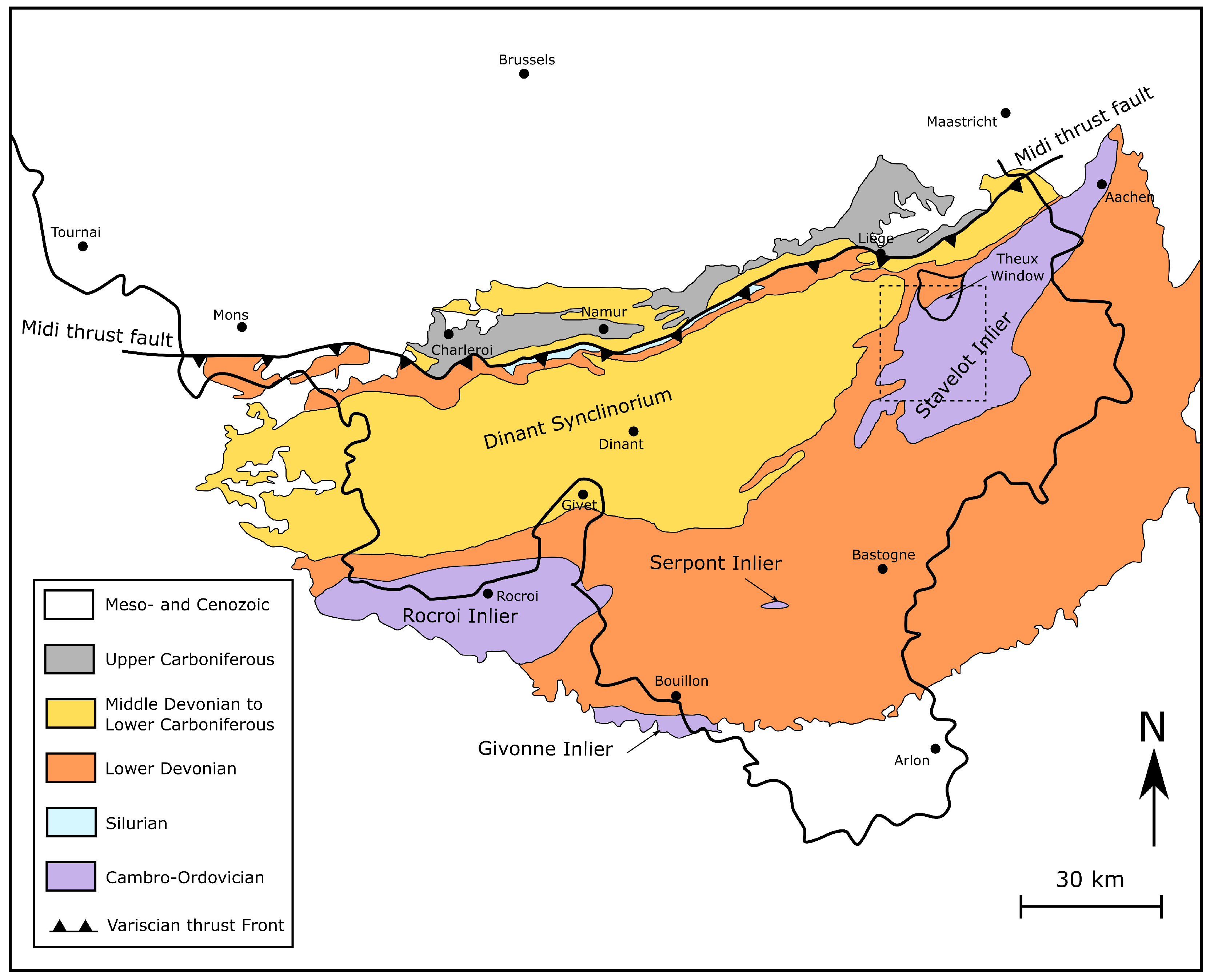
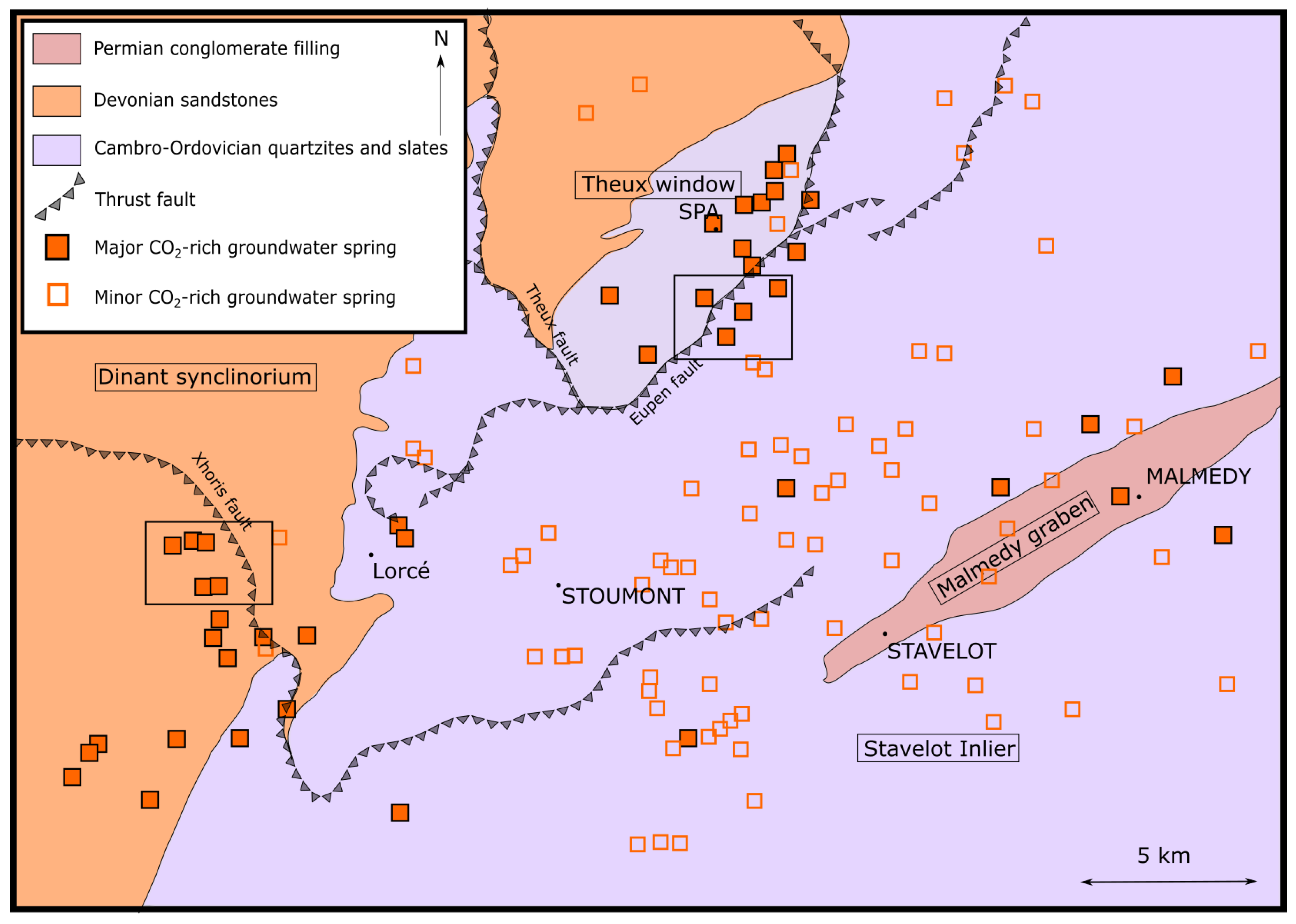
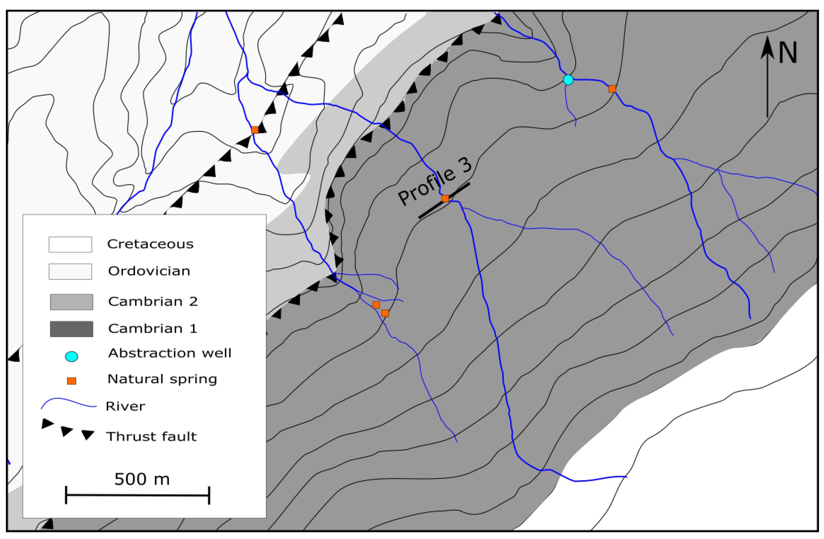
2. Geological Context
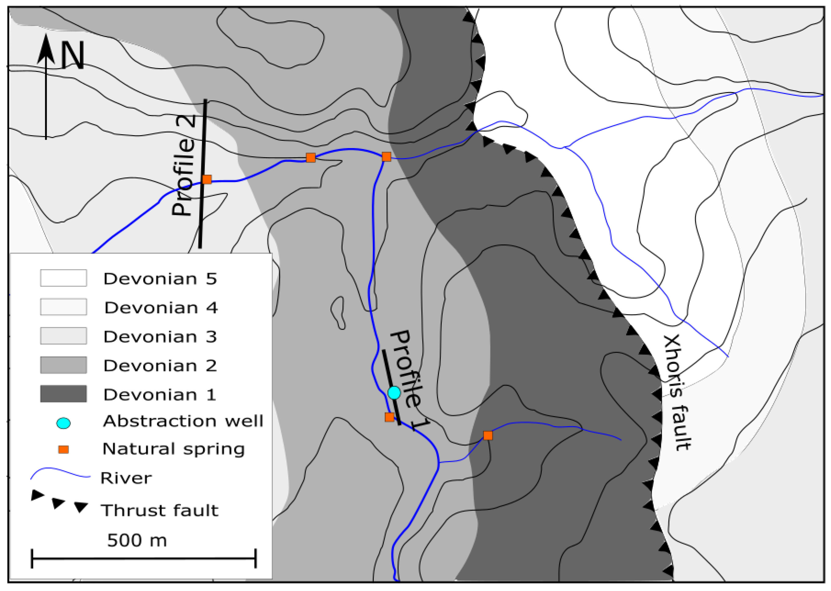
3. Experimental Sites
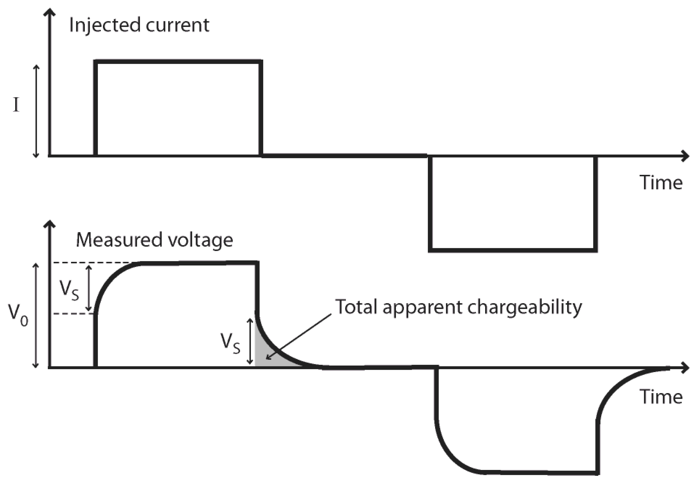
4. Materials and Methods
4.1. Acquisition Parameters
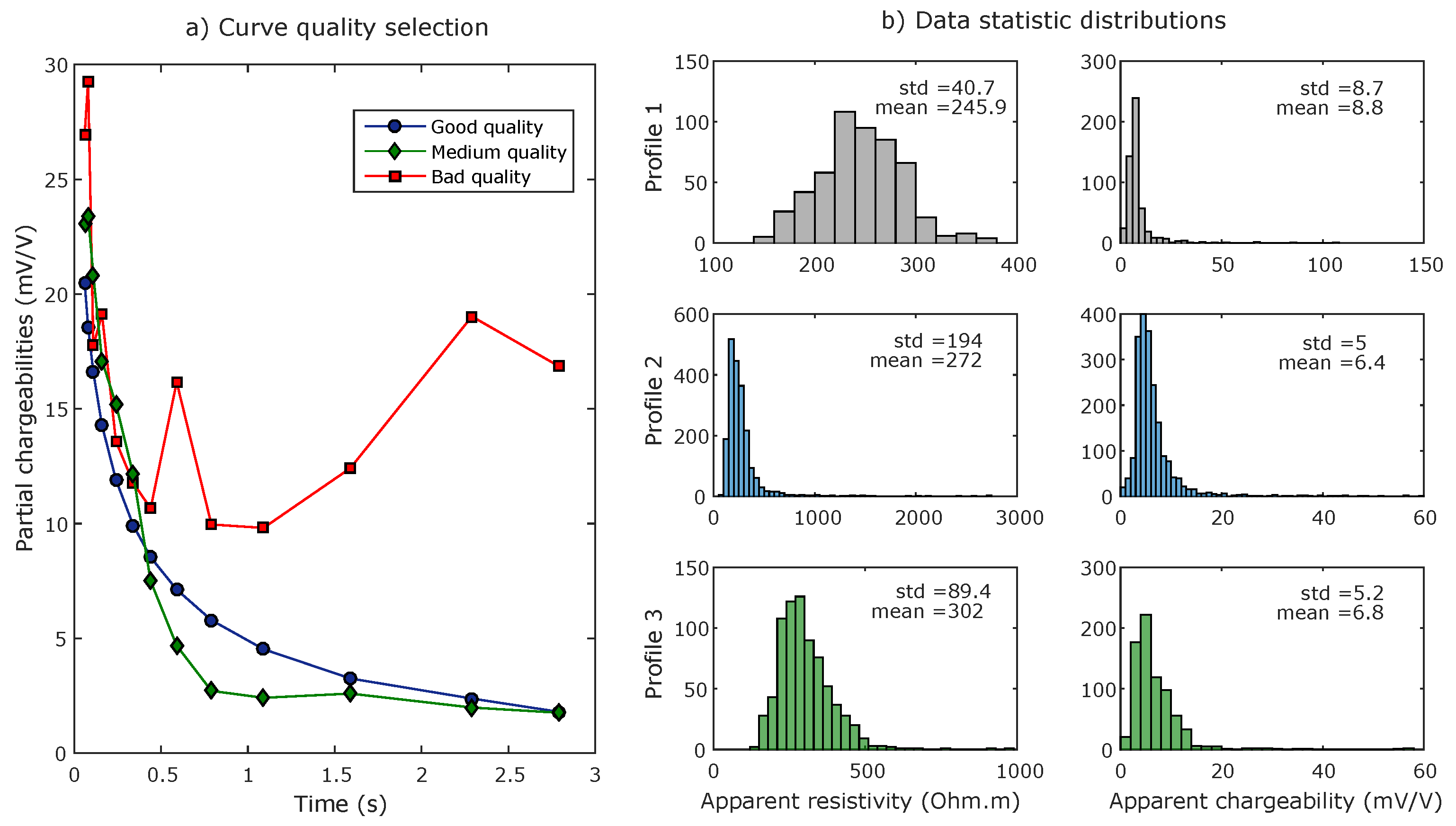
4.2. Data Processing and Inversion
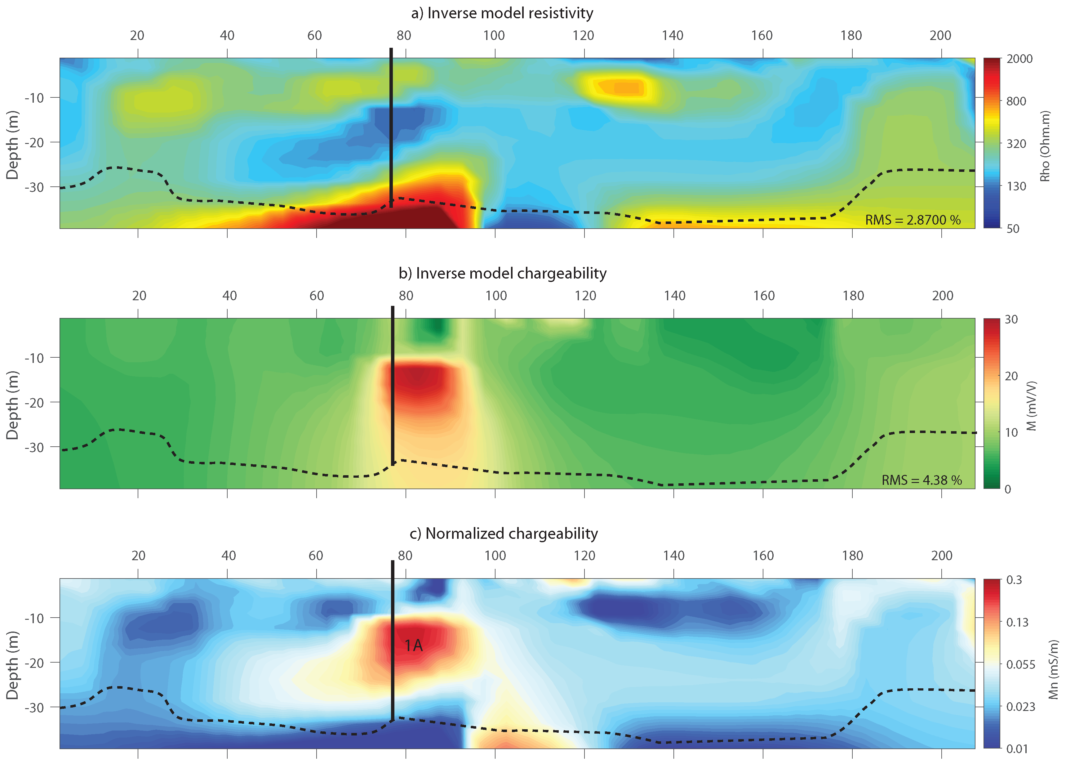
5. Results
5.1. Profile 1
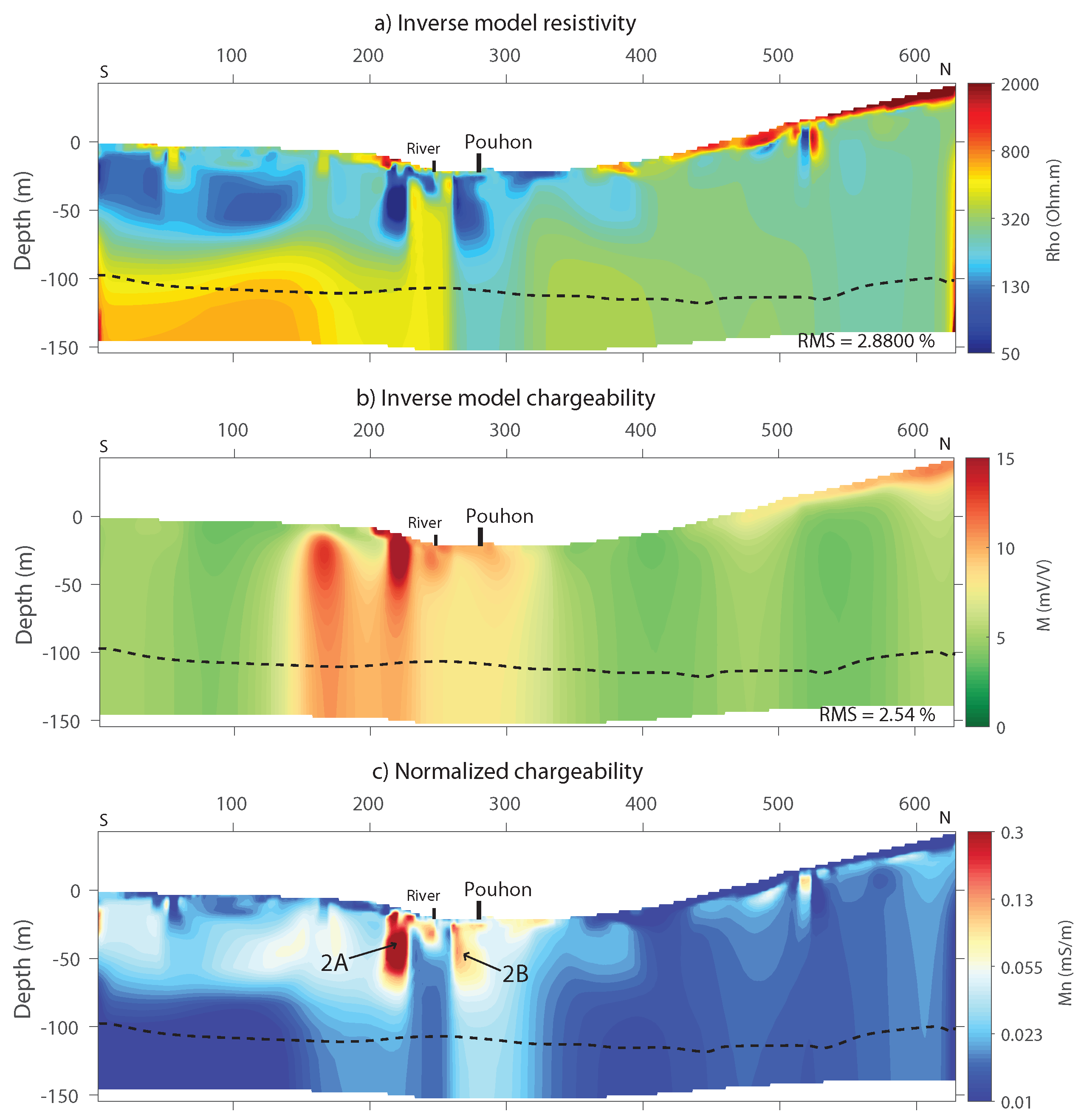
5.2. Profile 2
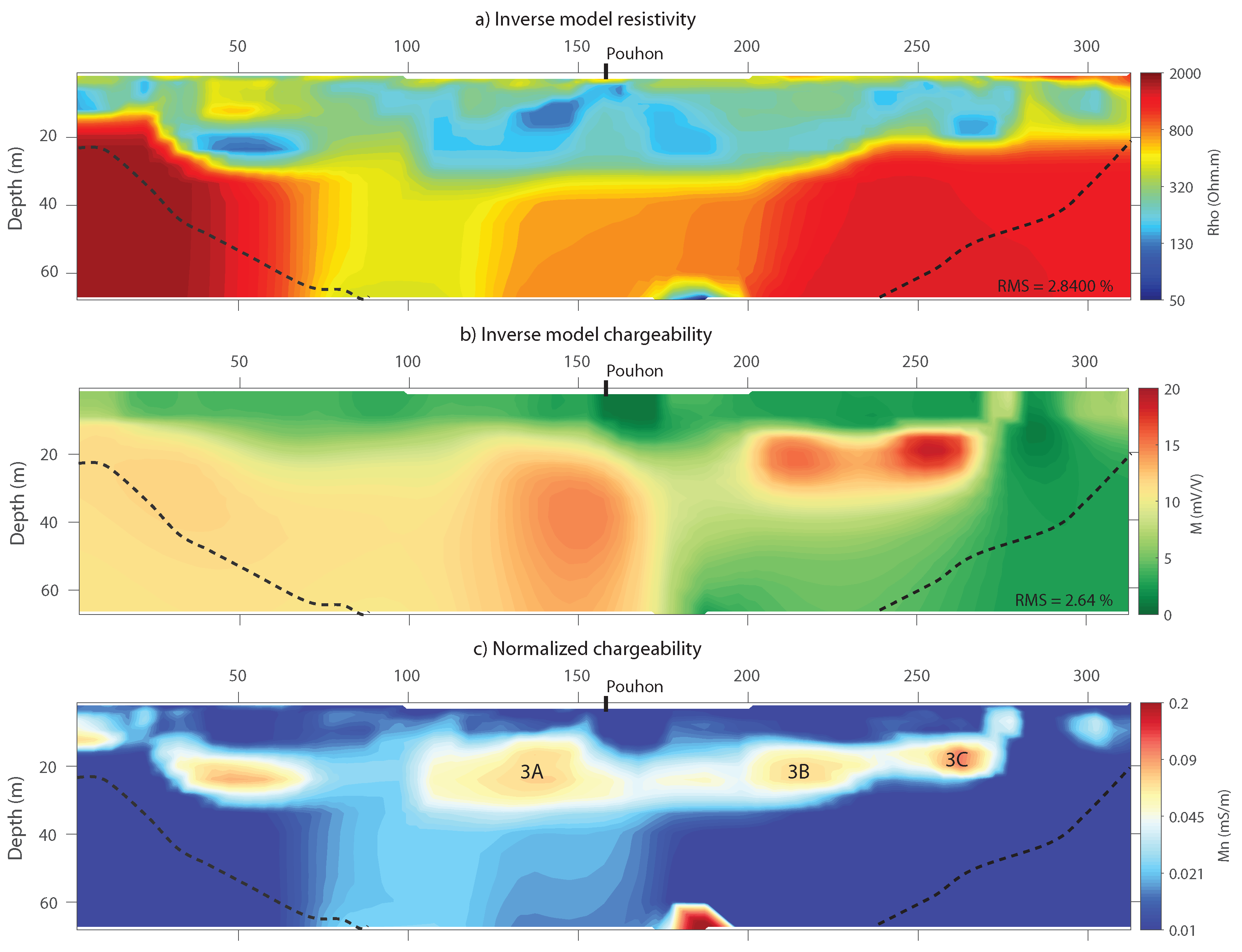
5.3. Profile 3
6. Discussion
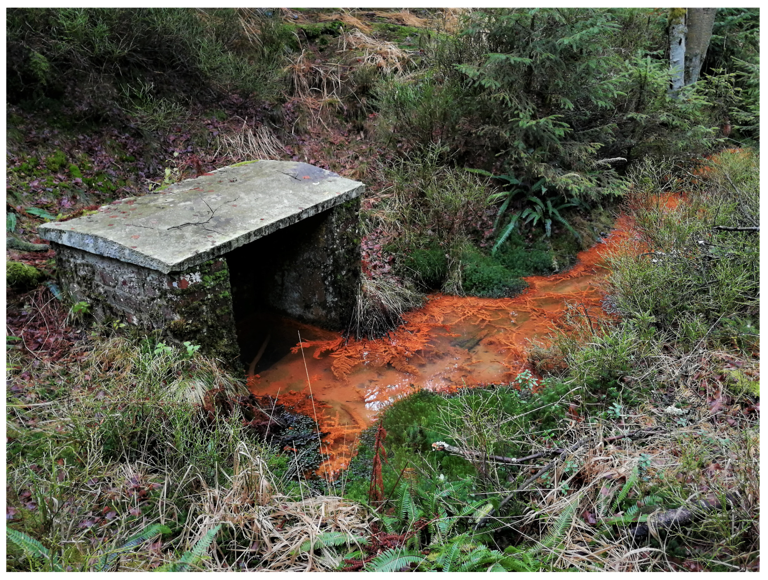
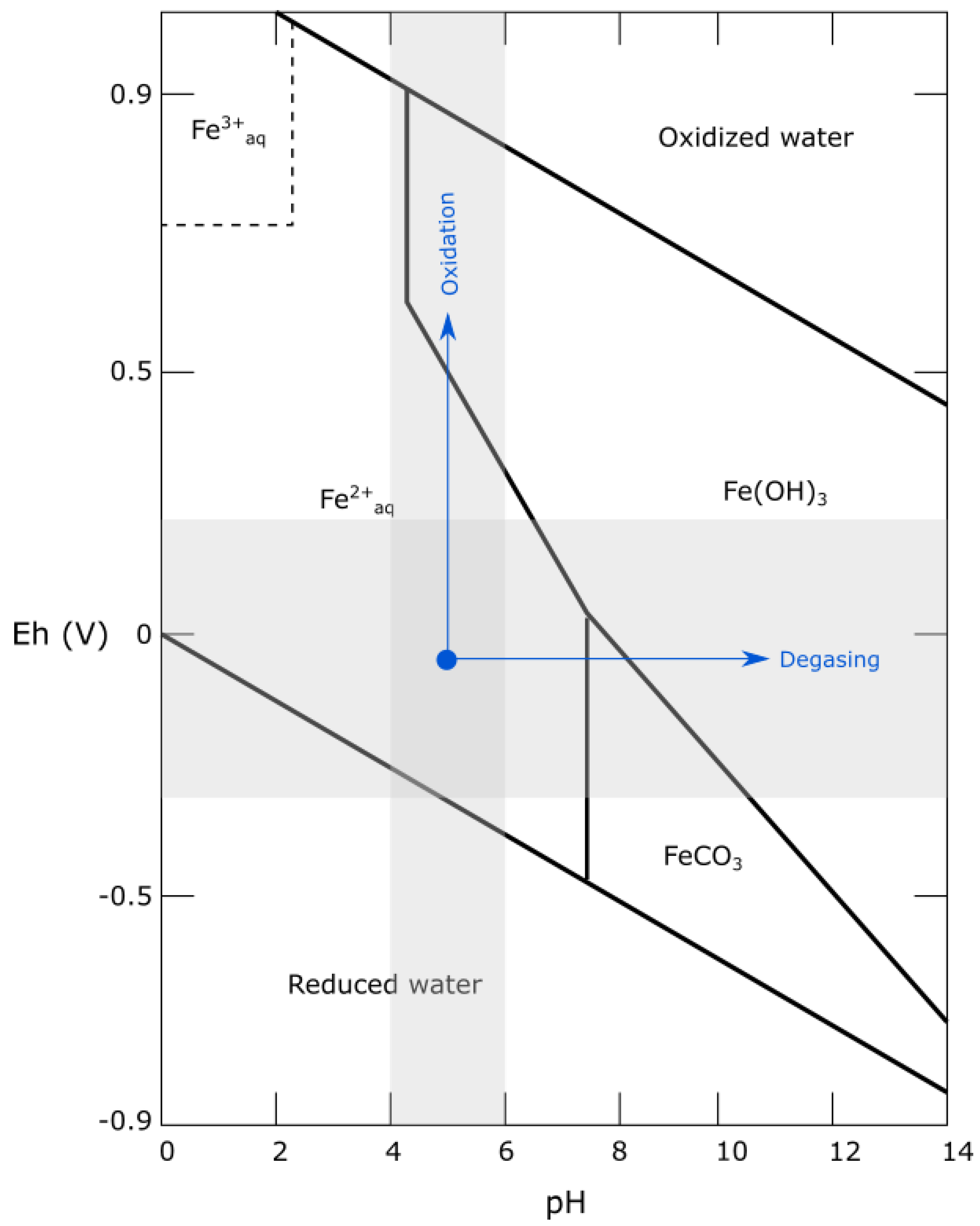
6.1. Iron Oxides and Hydroxides as Markers of CO-Rich Groundwater Circulation
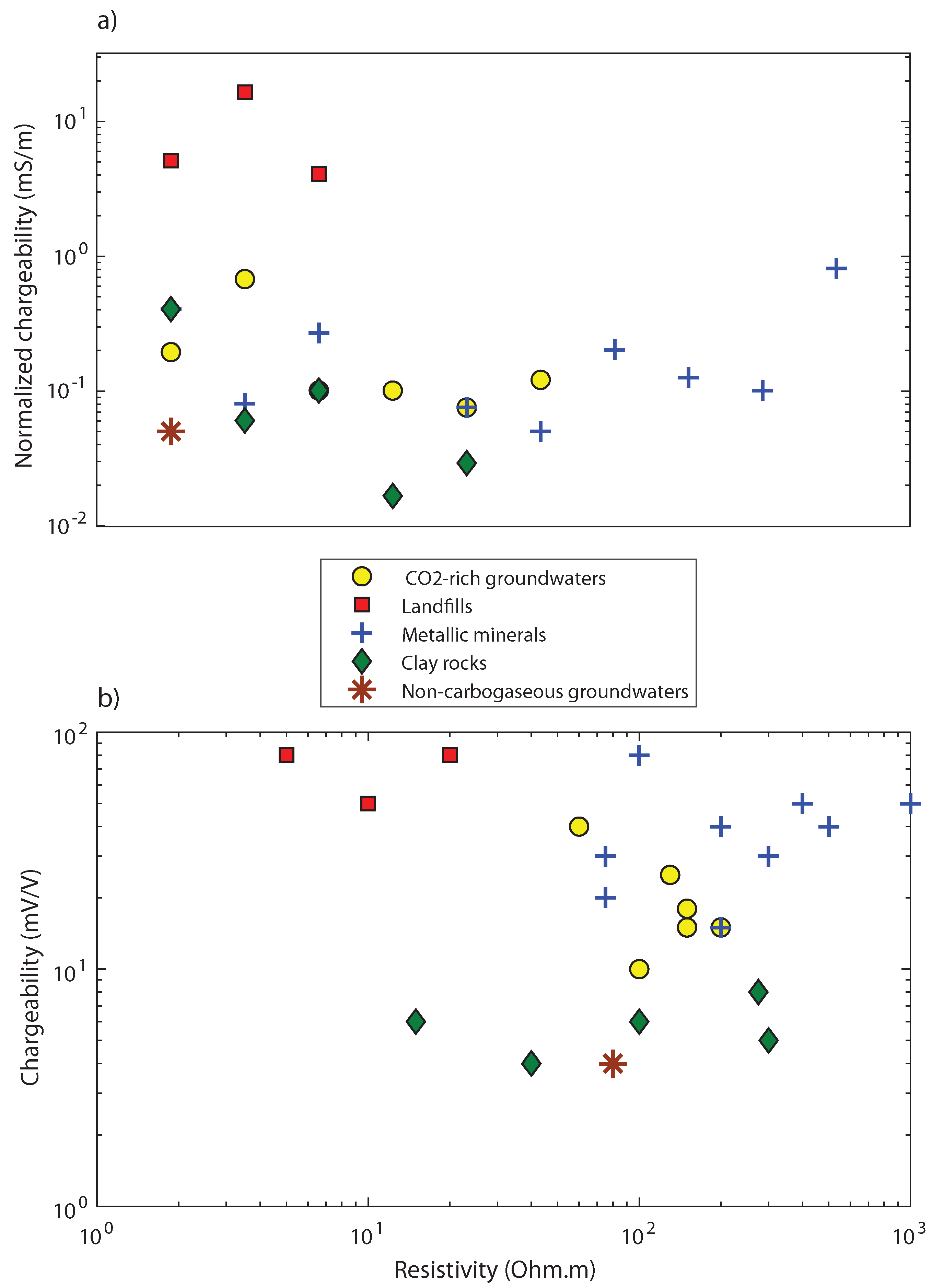
6.2. Geoelectric Signature of CO-Rich Groundwater Circulation
7. Conclusions and Further Research
Author Contributions
Funding
Conflicts of Interest
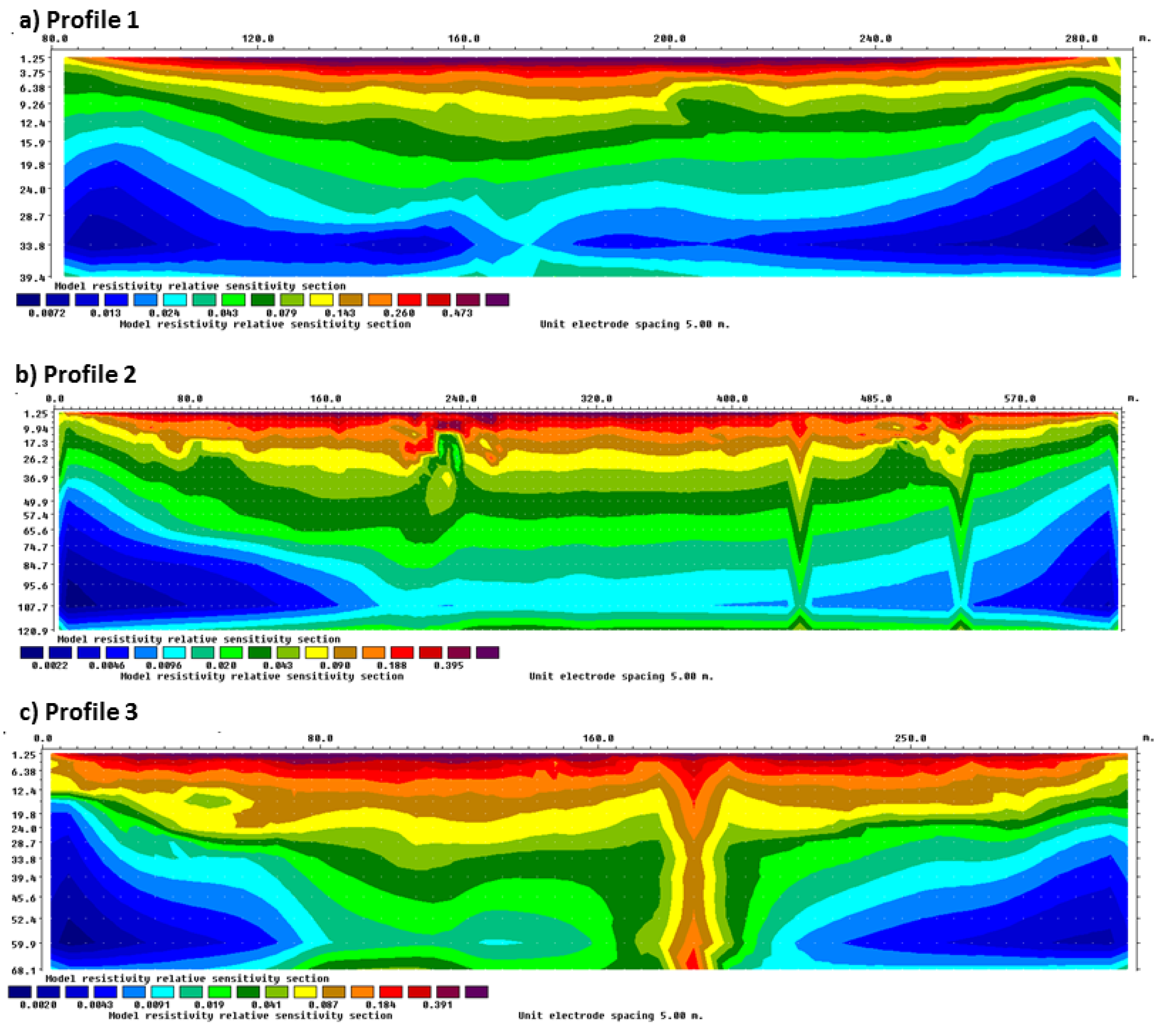
Appendix A. Sensitivity Distributions of ERT/TDIP Profiles

Appendix B. ERT/TDIP Anomalies Associated with Non-carbogaseous Groundwater

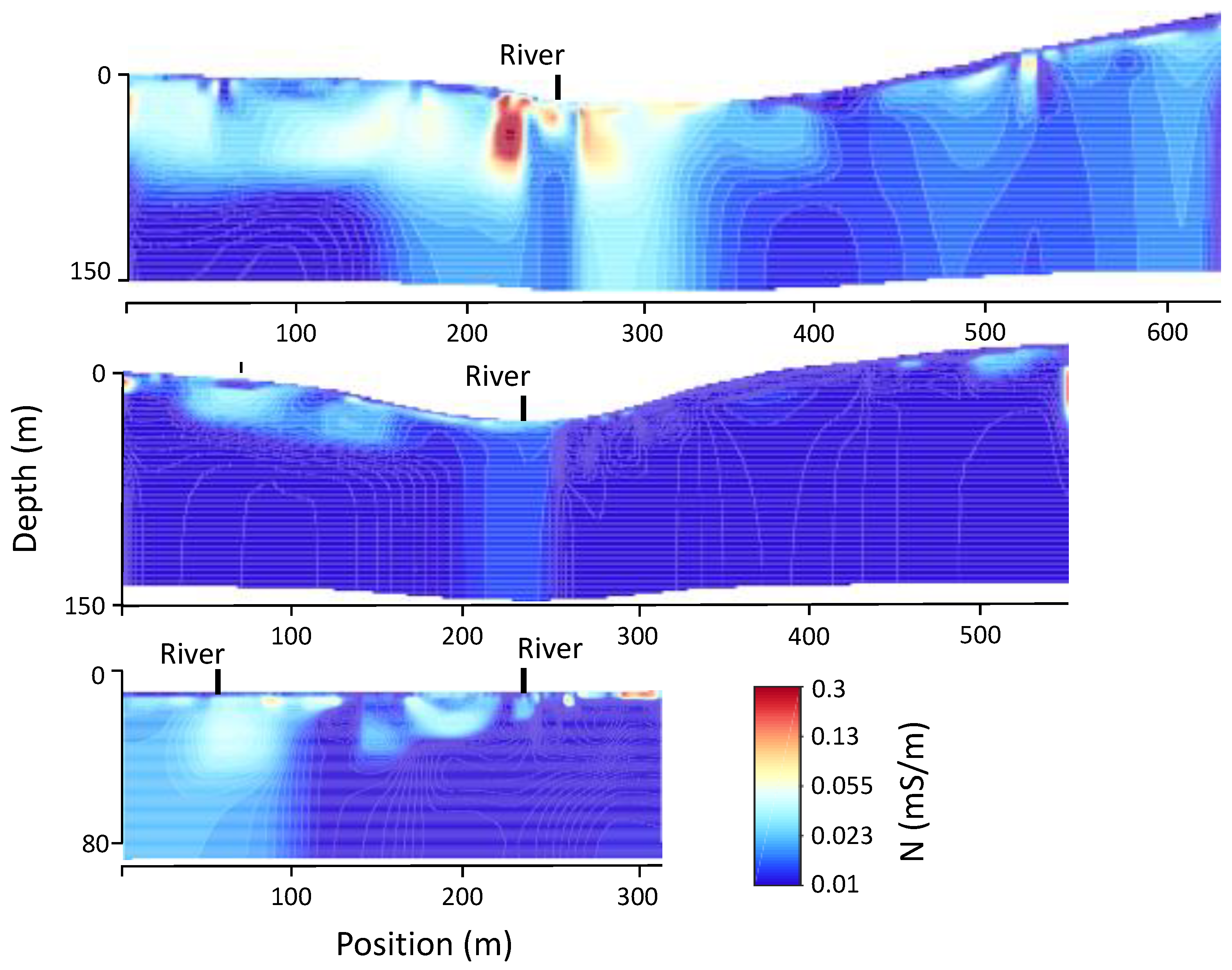
Appendix C. Effect of the Presence of the River

References
- Dewandel, B.; Alazard, M.; Lachassagne, P.; Bailly-Compte, V.; Coueffe, R.; Grataloup, S.; Ladouche, B. Respective roles of the weathering profile and the tectonic fractures in the structures and functioning of crustalline thermo-mineral carbo-gaseous aquifers. J. Hydrol. 2017, 547, 690–707. [Google Scholar] [CrossRef]
- Marechal, J.; Lachassagne, P.; Ladouche, B.; Dewandel, B.; Lanini, S.; Strat, P.L.; Petelet-Giraud, E. Structure and hydrogeochemical functioning of a sparkling natural mineral water system determined using a multidisciplinary approach: A case study from southern France. Hydrogeol. J. 2014, 22, 47–68. [Google Scholar] [CrossRef] [Green Version]
- Goepel, A.; Lonschiniski, M.; Viereck, L.; Buchel, G.; Kukowski, N. Volcano-tectonic structures and CO2-degassing patterns in the Laccher See basin, Germany. Int. J. Earth Sci. 2015, 104, 1483–1495. [Google Scholar] [CrossRef]
- Lesniak, P.M. Origin of carbon dioxide and evolution of CO2-rich waters in the West Carapathians, Poland. Acta Geol. Pol. 1998, 48, 343–366. [Google Scholar]
- Grassa, F.; Capasso, G.; Favara, R.; Inguaggiato, S. Chemical and isotopic composition of waters and dissolved gases in some thermal springs of Sicily and adjacent volcanic islands, Italy. Pure Appl. Geophys. 2006, 163, 781–807. [Google Scholar] [CrossRef]
- Carreira, P.; Marques, J.; Carvalho, M.; Nunes, D.; da Silva, M.A. Carbon isotopes and geochemical processes in CO2-rich cold mineral water, N-Portugal. Environ. Earth Sci. 2014, 71, 2941–2953. [Google Scholar] [CrossRef]
- Tassi, F.; Vaselli, O.; Moratti, G.; Piccardi, L.; Minissle, A.; Poreda, R.; Huertas, A.D.; Bendkik, A.; Chenakeb, M.; Tedesco, D. Fluid geochemistry versus tectonic setting: The case study of Morocco. Geol. Soc. Lond. Spec. Publ. 2006, 262, 131–145. [Google Scholar] [CrossRef]
- Shugg, A. Hepburn Spa: Cold carbonated mineral waters of Central Victoria, South Eastern Australia. Environ. Geol. 2008, 58, 1663–1673. [Google Scholar] [CrossRef]
- Choi, H.; Woo, N.C. Natural analogue monitoring to estimate the hydrochemical change of groundwater by the carboating process from the introduction of CO2. J. Hydrol. 2018, 562, 318–334. [Google Scholar] [CrossRef]
- Honnegger, J.; Gadalia, A. Exploitation des eaux minérales carbo-gazeuses. Houille Blanche 1995, 2, 106–110. [Google Scholar] [CrossRef] [Green Version]
- Rubin, Y.; Hubbard, S. Hydrogeophysics; Springer Science & Business Media: Cham, Switzerland, 2006; Volume 50. [Google Scholar]
- Gao, Q.; Shang, Y.; Hasan, M.; Jin, W.; Yang, P. Evaluation of a weathered rock aquifer using ERT method in South Guangdong, China. Water 2018, 10, 293. [Google Scholar] [CrossRef] [Green Version]
- Robinson, J.; Slater, L.; Johnson, T.; Shapiro, A.; Tiedeman, C.; Ntarlagiannis, D.; Lane, J. Imaging pathways in fractured rock using three-dimensional electrical resistivity tomography. Groundwater 2016, 5, 186–201. [Google Scholar] [CrossRef] [PubMed]
- Robert, T.; Dassargues, A.; Brouyère, S.; Kaufmann, O.; Hallet, V.; Nguyen, F. Assessing the contribution of electrical resistivity tomography (ERT) and self-potential (SP) methods for a water well drilling program in fractured/karstified limestones. J. Appl. Geophys. 2011, 75, 42–53. [Google Scholar] [CrossRef]
- Ball, L.B.; Ge, S.; Caine, J.S.; Revil, A.; Jardani, A. Constraining fault-zone hydrogeology through integrated hydrological and geoelectrical analysis. Hydrogeol. J. 2010, 18, 1057–1067. [Google Scholar] [CrossRef]
- Yadav, G.; Singh, S. Integrated resistivity surveys for delineation of fractures for groundwater exploration in hard rock areas. J. Appl. Geophys. 2007, 62, 301–312. [Google Scholar] [CrossRef]
- Nguyen, F.; Sand, D.; Jongmans, S.G.; Pirard, E.; Loke, M. Image processing of 2D resistivity data for imaging faults. J. Appl. Geophys. 2005, 57, 260–277. [Google Scholar] [CrossRef]
- Binley, A.; Kemna, A. DC resistivity and induced polarization methods. In Hydrogeophysics; Springer: Cham, Switzerland, 2005; pp. 129–156. [Google Scholar]
- Revil, A.; Aal, G.A.; Atekwana, E.; Mao, D.; Florsh, N. Induced polarization response of porous media with metallic particles—2: Comparison with a broad database of experimental data. Geophysics 2015, 80, 539–552. [Google Scholar] [CrossRef]
- Mao, D.; Revil, A. Induced polarization response of porous media with metallic particles—Part 3: A new approach to time-domain induced polarization tomography. Geophysics 2016, 81, 345–357. [Google Scholar] [CrossRef]
- Waxman, H.V.M. Induced polarization of shaly sands. Geophysics 1984, 49, 1267–1287. [Google Scholar]
- Weller, A.; Slater, L.; Nordsiek, S. On the relationship between induced polarization and surface conductivity: Implications for petrophysical interpretation of electrical measurements. Geophysics 2013, 78, 315–325. [Google Scholar] [CrossRef]
- Chelidze, T.; Gueguen, Y. Electrical spectroscopy of porous rocks: A review—I. Theoretical models. Geophys. J. Int. 1999, 137, 1–15. [Google Scholar] [CrossRef]
- Bleil, D. Induced polarization: A method of geophysical prospecting. Geophysics 1953, 18, 636–661. [Google Scholar] [CrossRef]
- Mansoor, N.; Slater, L. On the relationship between iron concentration and induced polarization in marsh soils. Geophysics 2006, 72, 1–5. [Google Scholar] [CrossRef]
- Moreira, C.; Borges, M.; Vieira, G.; Filho, W.; Montanheiro, M. Geological and geophysical data intergration for delimitation of mineralized areas in a supergene manganese deposits. Geofis. Int. 2012, 53, 403–416. [Google Scholar]
- Srigutomo, W.; Trimadona; Pratomo, P. 2D Resistivity and Induced Polarization Measurement for Manganese Ore Exploration. J. Phys. Conf. Ser. 2016, 739, 012138. [Google Scholar] [CrossRef]
- Carlson, N.R.; Hare, J.L.; Zonge, K.L. Buried landfill delineation with induced polarization: Progress and problems. In Proceedings of the SAGEEP, 14th EEGS Symposium on the Application of Geophysics to Engineering and Environmental Problems, Denver, CO, USA, 4–7 March 2001; Volume 20. [Google Scholar]
- Kemna, A.; Binley, A.; Slater, L. Crosshole IP imaging for engineering and environmental applications. Geophysics 2004, 69, 97–107. [Google Scholar] [CrossRef]
- Gazoty, A.; Fiandaca, G.; Pedersen, J.; Auken, E.; Christiansen, A. Mapping of landfills using time-domain spectral induced polarization data: The Eskelund case study. Surf. Geophys. 2012, 10, 575–586. [Google Scholar] [CrossRef] [Green Version]
- Dafflon, B.; Wu, Y.; Hubbard, S.; Birkholzer, J.; Daley, T.; Pugh, J.; Trautz, R. Monitoring CO2 intrusion and associated geochemical transformations in a shallow groundwater system using complex electrical methods. Environ. Sci. Technol. 2012, 47, 314–321. [Google Scholar] [CrossRef] [Green Version]
- Kremer, T.; Schmutz, M.; Agrinier, P.; Maineult, A. Laboratory monitoring of CO2 injection in saturated silica and carbonate sands using spectral induced polarization. Geophys. J. Int. 2016, 207, 1258–1272. [Google Scholar] [CrossRef]
- Aizebeokhai, A.; Oyeyemi, K.; Joel, E. Electrical resistivity and induced-polarization imaging for groundwater exploration. In Proceedings of the SEG Technical Program Expanded Abstracts; Dallas, TX, USA, 16–21 October 2016, Society of Exploration Geophysicists: Houston, TX, USA, 2016; pp. 2487–2491. [Google Scholar]
- Chrindja, F.J.; Dahlin, T.; Steinbruch, F. Reconstructing the formation of a costal aquifer in Nampula province, Mozambique, from ERT and IP methods for water prospection. Environ. Earth Sci. 2017, 76, 36. [Google Scholar] [CrossRef] [Green Version]
- Levy, L.; Maurya, P.; Byrdina, S.; Vandemeulebrouck, J.; Sigmundsson, F.; Arnason, K.; Labazuy, P. Electrical Resistivity Tomography and Time-Domain Induced Polarization field investigations of geothermal areas at Krafla, Iceland: Comparison to borehole and laboratory frequency-domain electrical observations. Geophys. J. Int. 2019, 218, 1469–1489. [Google Scholar] [CrossRef] [Green Version]
- Wollast, R.; Wollast, A. Etude géochimique des eaux carbogazeuses de la région de Stoumont. Les Eaux Souterraines en WALLONIE, Bilan et Perspectives-ESO 87; Région Wallonne of Belgium: Namur, Belgium, 1987. [Google Scholar]
- Oldenburg, D.; Li, Y. Inversion for applied geophysics: A tutorial. Investig. Geophys. 2005, 13, 89–150. [Google Scholar]
- Airo, M. Geophysical signatures of mineral deposit types. Geol. Surv. Finl. Spec. Pap. 2015, 58, 9–70. [Google Scholar]
- King, A.; Milkereit, B. Review of geophysical technology for Ni-Cu-PGE deposits. In Proceedings of Fifth Decennial International Conference on Mineral Exploration; Toronto, ON, Canada, 9–12 September 2007, Decennial Mineral Exploration Conferences: Toronto, ON, Canada, 2007; Volume 7, pp. 647–665. [Google Scholar]
- Vanbrabant, Y.; Braun, J.; Jongmans, D. Models of passive margin inversion: Implications for the Rhenohercynian fold-and-thrust belt, Belgium and Germany. Earth Planet. Sci. Lett. 2002, 202, 15–29. [Google Scholar] [CrossRef]
- Hance, L.; Dejonghe, L.; Ghysel, P.; Laloux, M.; Mansy, J. Influence of heterogeneous lithostructural layering on orogenic deformation in the Variscan Front Zone (eastern Belgium). Tectonophysics 1999, 309, 161–177. [Google Scholar] [CrossRef]
- Goemaere, E.; Demarque, S.; Dreeseen, R.; Declercq, P.Y. The Geological and Cultural Heritage of the Caledonien Stavelot-Venn Massif, Belgium. Geoheritage 2016, 8, 211–233. [Google Scholar] [CrossRef]
- Belanger, I.; Delaby, S.; Delcambre, B.; Ghysel, P.; Hennebert, M.; Laloux, M.; Marion, J.; Mottequin, B.; Pingot, J. Redéfinition des unités structurales du front varisque utilisées dans le cadre de la nouvelle Carte Géologique de Wallonie (Belgique). Geol. Belg. 2012, 15, 169–175. [Google Scholar]
- Herbosch, A.; Liégeois, J.P.; Pin, C. Coticules of the Belgian type area (Stavelot-Venn Massif): Limy turbidites within the nascent Rheic oceanic basin. Earth-Sci. Rev. 2016, 159, 186–214. [Google Scholar] [CrossRef]
- Geukens, F. Strike skip deformation des deux cotés du Graben de Malmédy. Ann. De La Société Géologique De Belg. 1995, 118, 139–146. [Google Scholar]
- Debbaut, V.; Cajot, O.; Ruthy, I.; Dassargues, A.; Hanson, A.; Bouezmarni, M. Aquifères de l’Ardenne; Academia Press: Gent, Belgium, 2014. [Google Scholar]
- Blondel, A. Développement des méThodes géOphysiques Électriques pour la Caractérisation des Sites et Sols Pollués aux Hydrocarbures. Ph.D. Thesis, Ecole Doctorale Montaigne-Humanités, Pessac, France, 2014. [Google Scholar]
- Schön, J. Physical Properties of Rocks: Fundamentals and Principles of Petrophysics; Elsevier: Amsterdam, The Netherlands, 1996; Volume 65. [Google Scholar]
- Slater, L.; Lesmes, D. Electrical-hydraulic relationships observed for unconsolidated sediments. Water Resour. Res. 2002, 38, 31. [Google Scholar] [CrossRef]
- Aster, R.; Borchers, B.; Thurber, C. Parameter Estimation and INVERSE Problems; Elsevier: Amsterdam, The Netherlands, 2018. [Google Scholar]
- Binley, A.; Slater, L.; Fukes, M.; Cassiani, G. Relationship between spectral induced polarization and hydraulic properties of saturated and unsaturated sandstone. Water Resour. Res. 2005, 41, 12. [Google Scholar] [CrossRef]
- Gazoty, A.; Fiandaca, G.; Pedersen, J.; Auken, E.; Christiansen, A. Data repeatability and acquisition techniques for time-domain spectral induced polarization. Surf. Geophys. 2013, 11, 391–406. [Google Scholar] [CrossRef] [Green Version]
- Loke, M.; Kuras, O.; Chambers, J.; Rucker, D.; Wilkinson, P. Instrumentation, Electrical Resistivity. In Encyclopedia of Solid Earth Geophysics; Gupta, H.K., Ed.; Springer International Publishing: Cham, Switzerland, 2020; pp. 1–7. [Google Scholar]
- Dahlin, T.; Zhou, B. Multiple-gradient array measurements for multichannel 2D resistivity imaging. Surf. Geophys. 2006, 4, 113–123. [Google Scholar] [CrossRef] [Green Version]
- Aizebeokhai, A.; Oyeyemi, K. The use of the multiple-gradient array for geoelectrical resistivity and induced polarization imaging. J. Appl. Geophys. 2014, 111, 364–376. [Google Scholar] [CrossRef]
- Dahlin, T.; Leroux, V.; Nissen, J. Measuring techniques in induced polarisation imaging. J. Appl. Geophys. 2002, 50, 279–298. [Google Scholar] [CrossRef] [Green Version]
- Loke, M.; Barker, R. Rapid least-squares inversion of apparent resistivity pseudosections by a quasi-Newton method. Geophys. Prospect. 1996, 44, 131–152. [Google Scholar] [CrossRef]
- Loke, M.; Chambers, J.; Ogilvy, R. Inversion of 2D spectral induced polarization imaging data. Geophys. Prospect. 2006, 54, 287–301. [Google Scholar] [CrossRef]
- Caterina, D.; Beaujean, J.; Robert, T.; Nguyen, F. A comparison study of different image appraisal tools for electrical resistivity tomogrphy. Surf. Geophys. 2013, 11, 639–657. [Google Scholar] [CrossRef]
- MacNeill, J. Electrical Conductivity of Soils and Rocks; Geonics Limited: Mississauga, ON, Canada, 1980. [Google Scholar]
- Portal, A.; Belle, P.; Mathieu, F.; Lachassagne, P.; Brisset, N. Identification and Characterization of Hard Rocks Weathering Profile by Electrical Resistivity Imaging. In Proceedings of the 23rd European Meeting of Environmental and Engineering Geophysics. European Association of Geoscientists & Engineers, Malmo, Sweden, 3–7 September 2017; 2017, pp. 1–5. [Google Scholar]
- Lamberty, P.; Geukens, F.; Marion, J. Notice explicative de la carte géologique Stavelot-Malmédy (50 5-6). Available online: https://orbi.uliege.be/handle/2268/207547 (accessed on 10 May 2020).
- Modelska, M.; Buczyński, S.; Błachowicz, M.; Heidemann, M.; Grzęda, O.; Karkoszka, Ł. The Mofetta Tylicz–an example of carbonated water springs in the area of Tylicz (Beskid Sądecki, the Carpathians). Geosci. Rec. 2015, 1, 27–33. [Google Scholar] [CrossRef]
- Operacz, A.; Wąsik, E.; Hajduga, M.; Chmielowski, K. Therapeutic water in the Poprad Valley–the newest development in the polish outer Carpathians. Pol. J. Environ. Stud. 2018, 27, 1207–1217. [Google Scholar] [CrossRef]
- Jeong, C.H.; Kim, H.J.; Lee, S.Y. Hydrochemistry and genesis of CO2-rich springs from Mesozoic granitoids and their adjacent rocks in South Korea. Geochem. J. 2005, 39, 517–530. [Google Scholar] [CrossRef] [Green Version]
- Chae, G.; Yu, S.; Jo, M.; Choi, B.Y.; Kim, T.; Koh, D.C.; Yun, Y.Y.; Yun, S.T.; Kim, J.C. Monitoring of CO2-rich waters with low pH and low EC: An analogue study of CO2 leakage intro into shallow aquifers. Environ. Eath Sci. 2016, 75, 15. [Google Scholar] [CrossRef]
- Langmuir, D. Aqueous Environmental Geochemistry; Prentice Hall: Upper Saddle River, NJ, USA, 1997. [Google Scholar]
- Aal, G.A.; Atekwana, E.; Revil, A. Geophysical signatures of disseminated iron minerals: A proxy for understanding subsurface biophysicochemical processes. J. Geophys. Res. Biogeosci. 2014, 119, 1831–1849. [Google Scholar]
- Slater, L.; Choi, J.; Wu, Y. Electrical properties of iron-sand columns: Implications for induced polarization investigation and performance monitoring of iron-wall barriers. Geophysics 2005, 70, G87–G94. [Google Scholar] [CrossRef]
- Evrard, M.; Dumont, G.; Hermans, T.; Chouteau, M.; Francis, O.; Pirard, E.; Nguyen, F. Geophysical Investigation of the Pb–Zn Deposit of Lontzen–Poppelsberg, Belgium. Minerals 2018, 8, 233. [Google Scholar] [CrossRef] [Green Version]
- Moreira, C.; Borssatto, K.; Ilha, L.; Santos, S.; Rosa, F. Geophysical modeling in gold deposit through DC Resistivity and Induced Polarization methods. REM-Int. Eng. J. 2016, 69, 293–299. [Google Scholar] [CrossRef]
- Okay, G.; Cosenza, P.; Ghorbani, A.; Camerlynck, C.; Cabrera, J.; Florsch, N.; Revil, A. Localization and characterization of cracks in clay-rocks using frequency and time-domain induced polarization. Geophys. Prospect. 2013, 61, 134–152. [Google Scholar] [CrossRef]
- Krahenbuhl, R.; Hitzman, M. Geophysical modeling of two willemite deposits, Vazante (Brazil) and Beltana (Australia). In SEG Technical Program Expanded Abstracts 2004; Society of Exploration Geophysicists: Houston, TX, USA, 2004; pp. 1187–1190. [Google Scholar]
- Dakir, I.; Benamara, A.; Aassoumi, H.; Ouallali, A.; Bahammou, Y.A. Application of Induced Polarization and Resistivity to the Determination of the Location of Metalliferous Veins in the Taroucht and Tabesbaste Areas (Eastern Anti-Atlas, Morocco). Int. J. Geophys. 2019, 2019, 1–11. [Google Scholar] [CrossRef] [Green Version]
- Pardo, O.; Gretta, C.; Alexander, E.; Iraida, M.; Pintor, B. Geophysical exploration of disseminated and stockwork deposits associated with plutonic intrusive rock: A case study on the eastern flank of Colombia’s western cordillera. Earth Sci. Res. J. 2012, 16, 11–23. [Google Scholar]
- Sultan, S.; Mansour, S.; Santos, F.; Helaly, A. Geophysical exploration for gold and associated minerals, case study: Wadi El Beida area, South Eastern Desert, Egypt. J. Geophys. Eng. 2009, 6, 345–356. [Google Scholar] [CrossRef]
- Azis, A.; Zamhuri, M.; Rais, M.; Aswad, S.; Patiung, O.; Sudianto, Y. Identify the Distribution of Galena using Induced Polarization and Resistivity Methods in central of Lombok, West Nusa Tenggara. In Proceedings of the IOP Conference Series: Earth and Environmental Science; Makassar, Indonesia, 1–2 November 2018, IOP Publishing: Bristol, UK, 2019; Volume 279. [Google Scholar]
- Amaya, A.G.; Dahlin, T.; Barmen, G.; Rosberg, J.E. Electrical resistivity tomography and induced polarization for mapping the subsurface of alluvial fans: A case study in Punata (Bolivia). Geosciences 2016, 6, 51. [Google Scholar] [CrossRef] [Green Version]
- Yusof, M.A.A.; Ismail, N.; Muztaza, N. The Application of 2D Resistivity and Induced Polarization Methods for Slope Study at Penang Island, Malaysia. In Proceedings of the SEGJ 136th (Spring) Conference; Tokyo, Japan, 5–7 June 2017, The Society of Exploration Geophysicists of Japan: Tokyo, Japan, 2017. [Google Scholar]
- Dahlin, T. Application of Resistivity-IP to Mapping of Groundwater Contamination and Buried Waste; Geophysical Association of Ireland: Dublin, Ireland, 2012; p. 6. [Google Scholar]
- Leroux, V.; Dahlin, T.; Svensson, M. Dense resistivity and induced polarization profiling for a landfill restoration project at Härlöv, Southern Sweden. Waste Manag. Res. 2007, 25, 49–60. [Google Scholar] [CrossRef] [PubMed] [Green Version]
- Dahlin, T.; Rosqvist, H.; Leroux, V. Resistivity-IP mapping for landfill applications. First Break 2010, 28, 101–105. [Google Scholar]
- Johansson, B.; Jones, S.; Dahlin, T.; Flyhammar, P. Comparisons of 2D-and 3D-inverted resistivity data as well as of resistivity-and IP-surveys on a landfill. In Proceedings of the Near Surface 2007-13th EAGE European Meeting of Environmental and Engineering Geophysics, Istanbul, Turkey, 3–5 September 2007. [Google Scholar]
- Santos, F.A.M.; Almeida, E.P.; Castro, R.; Nolasco, R.; Mendes-Victor, L. A hydrogeological investigation using EM34 and SP surveys. Earth Planets Space 2002, 54, 655–662. [Google Scholar] [CrossRef] [Green Version]
- Marques, J.; Santos, M.F.; Graça, R.; Castro, R.; Aires-Barros, L.; Victor, L.M. A geochemical and geophysical approach to derive a conceptual circulation model of CO 2-rich mineral waters: A case study of Vilarelho da Raia, northern Portugal. Hydrogeol. J. 2001, 9, 584–596. [Google Scholar]


| Material Type | Chargeability (mV/V) | Material Type | Chargeability (mV/V) |
|---|---|---|---|
| Pyrrhotite | ∼10 | 20% Sulphides | 2000–3000 |
| Pentlandite | ∼10 | 8%–20% Sulphides | 1000–2000 |
| Pyrite | 13.4 | 2%–8% Sulphides | 500–1000 |
| Copper | 12.3 | Volcanic tuffs | 300–800 |
| Graphite | 11.2 | Sandstone, Siltstone | 100–500 |
| Chalcopyrite | 9.4 | Dense volcanic rocks | 100–500 |
| Magnetite | 2.2 | Shale | 50–100 |
| Galena | 3.7 | Granite, Granodiorite | 10–50 |
| Hematite | 0.0 | Limestone, Dolomite | 10–20 |
| Profile 1 | Profile 2 | Profile 3 | |
|---|---|---|---|
| Length (m) | 315 | 615 | 315 |
| ♯ electrodes | 64 | 126 | 64 |
| Electrode spacing (m) | 5 | 5 | 5 |
| Presence of spring or abstraction well | Spring + Well (9 m/h) | Spring | Spring |
| ♯ iterations | 4 | 4 | 4 |
| RMS resistivity (%) | 2.87 | 2.88 | 2.84 |
| RMS chargeability (%) | 4.38 | 2.54 | 2.64 |
| Parameter | Profile 1 | Profile 2 | Profile 3 |
|---|---|---|---|
| Type of spring | Well | Pouhon | Pouhon |
| pH [-] | 5.9 | 5.8 | 5.6 |
| EC [S/cm] | 223 | 863 | 138 |
| Eh [mV] | 107 | 81 | |
| Ca2+ [mg/L] | 23.9 | 46.6 | 12.8 |
| Mg2+ [mg/L] | 10.76 | 30.3 | 4.5 |
| Na+ [mg/L] | 5.6 | 104 | 6.7 |
| K+ [mg/L] | 1.07 | 5.09 | 0.82 |
| [mg/L] | 7.1 | 9.8 | 8.6 |
| - [mg/L] | 100 | 414 | 59 |
| Fe total [mg/L] | 7.5 | 8.4 | 4.4 |
| Mn total [mg/L] | 0.48 | 0.76 | 0.14 |
| Dissolved [g/L] | 0.77 | 2.32 | 0.37 |
| Dissolved [g/L] | 2.5 | 5.8 |
| Reference | Context of Survey | Interpretation |
|---|---|---|
| [70] | Pb-Zn deposit | Sulphides (galena, sphalerite, pyrite and marcasite) |
| [26] | manganese deposits | manganese deposits (pyrite, chalcopyrite),Fe oxides |
| [71] | Gold exploration | Disseminated sulphides (pyrite, chalcopyrite),iron oxides |
| [34] | Water exploration | Sand with heavy minerals |
| [72] | Detecting cracks in clay rocks | 13% Pyrite in calcite rock |
| [73] | Detection of ore bodies | |
| [74] | Metalliferrous veins exploration | Presence of Barite and Galena |
| [75] | Plutonic rock mineral exploration | Sulphure mineralizations |
| [76] | Plutonic rock mineral exploration | Ore deposits |
| [77] | Galena exploration | Pyrite, chalcopyrite, galena |
| [35] | Volcanic geothermal area | Pyrite, iron oxides |
| [78] | Case study alluvial fans | High clay content |
| [47] | Hydrocarbon contamination | Clayey silt |
| [34] | Water exploration | Weathered rock leaching clay minerals |
| [79] | Slope study | Clay |
| [72] | Detecting cracks in clay rocks | Clay rocks |
| [80] | Landfill characterization | Clayey till |
| [52] | Mapping of lithotypes | Clay till |
| [81] | Landfill characterization | Waste, plastic and metal |
| [82] | Landfill characterization | Waste, soil with leachate |
| [80] | Landfill characterization | Waste and leachate |
| [83] | Landfill characterization | Waste |
© 2020 by the authors. Licensee MDPI, Basel, Switzerland. This article is an open access article distributed under the terms and conditions of the Creative Commons Attribution (CC BY) license (http://creativecommons.org/licenses/by/4.0/).
Share and Cite
Defourny, A.; Nguyen, F.; Collignon, A.; Jobé, P.; Dassargues, A.; Kremer, T. Induced Polarization as a Proxy for CO2-Rich Groundwater Detection—Evidences from the Ardennes, South-East of Belgium. Water 2020, 12, 1394. https://doi.org/10.3390/w12051394
Defourny A, Nguyen F, Collignon A, Jobé P, Dassargues A, Kremer T. Induced Polarization as a Proxy for CO2-Rich Groundwater Detection—Evidences from the Ardennes, South-East of Belgium. Water. 2020; 12(5):1394. https://doi.org/10.3390/w12051394
Chicago/Turabian StyleDefourny, Agathe, Frédéric Nguyen, Arnaud Collignon, Patrick Jobé, Alain Dassargues, and Thomas Kremer. 2020. "Induced Polarization as a Proxy for CO2-Rich Groundwater Detection—Evidences from the Ardennes, South-East of Belgium" Water 12, no. 5: 1394. https://doi.org/10.3390/w12051394