Uncertainty Assessment of Urban Hydrological Modelling from a Multiple Objective Perspective
by
 , and
, and
Bo Pang
1,2, 
Shulan Shi
1,2,
Gang Zhao
1,2,3,*,
Rong Shi
4,
Dingzhi Peng
1,2 and
Zhongfan Zhu
1,2 1
College of Water Sciences, Beijing Normal University, Beijing 100875, China
2
Beijing Key Laboratory of Urban Hydrological Cycle and Sponge City Technology, Beijing 100875, China
3
School of Geographical Science, University of Bristol, Bristol BS8 1SS, UK
4
Water in the Pearl River Planning Survey Design Co., Ltd. Beijing Branch, Beijing 100875, China
*
Author to whom correspondence should be addressed.
Water 2020, 12(5), 1393; https://doi.org/10.3390/w12051393
Submission received: 31 March 2020
/
Revised: 8 May 2020
/
Accepted: 12 May 2020
/
Published: 14 May 2020
(This article belongs to the Special Issue Advances in Hydrologic Forecasts and Water Resources Management )
Abstract
:The uncertainty assessment of urban hydrological models is important for understanding the reliability of the simulated results. To satisfy the demand for urban flood management, we assessed the uncertainty of urban hydrological models from a multiple-objective perspective. A multiple-criteria decision analysis method, namely, the Generalized Likelihood Uncertainty Estimation-Technique for Order Preference by Similarity to Ideal Solution (GLUE-TOPSIS) was proposed, wherein TOPSIS was adopted to measure the likelihood within the GLUE framework. Four criteria describing different urban stormwater characteristics were combined to test the acceptability of the parameter sets. The TOPSIS was used to calculate the aggregate employed in the calculation of the aggregate likelihood value. The proposed method was implemented in the Storm Water Management Model (SWMM), which was applied to the Dahongmen catchment in Beijing, China. The SWMM model was calibrated and validated based on the three and two flood events respectively downstream of the Dahongmen catchment. The results showed that the GLUE-TOPSIS provided a more precise uncertainty boundary compared with the single-objective GLUE method. The band widths were reduced by 7.30 m3/s in the calibration period, and by 7.56 m3/s in the validation period. The coverages increased by 20.3% in the calibration period, and by 3.2% in the validation period. The median estimates improved, with an increase of the Nash–Sutcliffe efficiency coefficients by 1.6% in the calibration period, and by 10.0% in the validation period. We conclude that the proposed GLUE-TOPSIS is a valid approach to assess the uncertainty of urban hydrological model from a multiple objective perspective, thereby improving the reliability of model results in urban catchment.
1. Introduction
Land use modifications accompanied by urbanization, including the decrease of vegetation cover, increase of impervious surfaces, and drainage channel modifications, result in changes in the characteristics of the surface runoff hydrograph [1,2]. Urban flooding and waterlogging are severe global environmental issues. Urban hydrological models play an important role in the planning and construction of urban drainage and flood control systems [3,4]. The Storm Water Management Model (SWMM), which was developed by the United States Environmental Protection Agency (EPA), has become one of the most popular urban hydrological models [5,6] in urban stormwater simulation.
Urban hydrological models typically require a large number of parameters, which are difficult or impossible to measure with sufficient accuracy, and must generally be estimated or evaluated from secondary information sources [7,8]. Hence, the obtained simulation results are typically laden with notable degrees of uncertainty [9]. Thus, various methods have been developed to assess the uncertainty in urban hydrological models, such as the Monte Carlo Markov chain [10,11], grey box model [12], Bayesian approach [13], and Generalized Likelihood Uncertainty Estimation (GLUE) method [14,15]. The selection of the objective function is critical for many of these uncertainty analysis methods. According to GLUE method, the objective function and acceptability threshold exert substantial influence on the final assessment results. The Nash–Sutcliffe Efficiency index (NSE) is widely used as the objective function in the GLUE method for urban hydrological models [16,17].
In 1998, Gupta et al. [18] proposed that hydrological model calibration inherently comprises multiple objectives, and that converting it into a single-objective model must involve some degree of subjectivity. The complexity of urban stormwater management comes from flood characteristics such as the flood volume, peak flood value, lag time, and overflow characteristics such as the overflow volume and duration. These characteristics concern different management system components [15,19] and are difficult to be captured by a single-objective function during model calibration and validation. Moreover, the adoption of the single-objective function introduces additional uncertainties in applications because it may consider unacceptable parameter sets [20,21]. The controversy can also be found in the use of informal likelihood measures based on the NSE, which involves subjective decisions [22].
This paper proposes a new framework for analyzing the uncertainty of an urban hydrological model. TOPSIS (evaluation technique for order performance by similarity to ideal solution), which is a multiple-criteria decision analysis (MCDA) method developed by Hwang and Yoon [23,24], was adopted as the likelihood criterion of the GLUE method using four important objective criteria in urban flood modelling. The proposed method was used to quantify the parameter uncertainties in the SWMM model and was applied to the Dahongmen (DHM) catchment located in Beijing, China. We attempted to improve the uncertainty assessment of an urban hydrological model by comprehensively investigating the performance of the parameter sets during simulation.
2. Methods
The proposed uncertainty analysis method is based on the GLUE framework, which was developed by Beven and Binley [25]. In the GLUE method, a likelihood measure is selected and calculated to reflect the goodness of fit between the model simulation and the observations. The model simulations are considered as non-behavioral when the values of the likelihood measures are lower than the cut-off threshold. The selection of the likelihood measure and cut-off threshold has been discussed in various papers, owing to the subjective decisions involved [22,26,27,28]. Because the single objective always involves some degree of subjectivity [18], the proposed method uses MCDA to carry out the likelihood measure; the critical points are summarized as follows:
- The performance of the parameter sets was comprehensively investigated by considering the threshold of each objective function. Only the parameter sets for which all objective function values exceeded their threshold were considered as behavioral.
- An integrated likelihood measure was carried out using TOPSIS, which was used as a weighting factor to derive the posterior probability density functions for both the parameters and the predictions. The prominent advantage of TOPSIS is that different types of objective functions can be easily integrated into a unified evaluation index by setting the benefit criteria and loss criteria.
The uncertainty assessment process can be described as follows:
- Instead of a unique likelihood measure, multiple thresholds from multiple criteria are used to determine the behavioral parameter sets. In urban stormwater management, not only the precision of the flood process but also the precision of the flood volume and flood peak is considered by the modeler [31]. A behavior parameter set should be able to achieve these objectives. The criteria typically used in flood prediction are as follows:andwhere is the observed flow, is the simulated flow, is the average measured flow, is the average simulated flow, and n is the number of the observed flow points.In the above formula, NSE is the widely used Nash–Sutcliffe efficiency index [32]. The flood volume bias (VB) and flood peak bias (PB) are the modified expressions for the flood volume and flood peak deviation [18,33], respectively. The parameter R represents the consistency between the observed flow and the simulated flow [34]. The threshold of these criteria can be defined with reference to practical demand [35]. The reasonable range of the four criteria is between 0 to 1. The optimum value of NSE and R is 1, and optimum value of VB and PB is 0, which means the simulation results of the model completely fit the measured results. In this study, the behavioral parameter sets whose likelihood values of the four criteria were greater than the corresponding thresholds were chosen for further analysis.
- TOPSIS, which is a well-known MCDA method and can provide the ranking order of all alternatives [36,37], was employed in the calculation of the aggregate likelihood value L() of the behavioral parameter set .In the TOPSIS method, the four criteria of all parameter sets should be normalized by the classification of the benefit and cost criterion, where the benefit criterion means that a larger value is more valuable, and vice-versa for the cost criterion [37]. In this study, NSE and R are benefit criteria, while VB and PB are cost criteria; xij is the ith criterion of the jth parameter set. For the benefit criteria, the normalized value (rij) is calculated as follows:For the cost criteria, the normalized value (rij) is calculated as follows:In many situations, the criterion should be weighted according its importance [36]. Because it is difficult to identify which criterion is more important, we assume that all criteria are equally important. The ideal solution and negative-ideal solution can be calculated as follows:Then, the separation of each alternative from the ideal and negative-ideal solutions are expressed, respectively, as follows:The aggregate likelihood value L() is evaluated by comparing the distance from the ideal solution and the distance from the negative-ideal solution:
- Finally, the predictions from the behavioral parameter sets are ranked in the order of the likelihood weights W(i), which is defined as follows:where N is the number of behavioral parameter sets. Additionally, the cumulative probability distribution for the ranked discharge predictions can be obtained as follows:where Q denotes the discharge, and Qi is the discharge prediction ranked at the ith position; n has the same meaning as in Equation (2). According to the cumulative probability distribution, the uncertainty bound can be obtained for a given certainty level.
3. Study Area and SWMM Model
3.1. Study Area
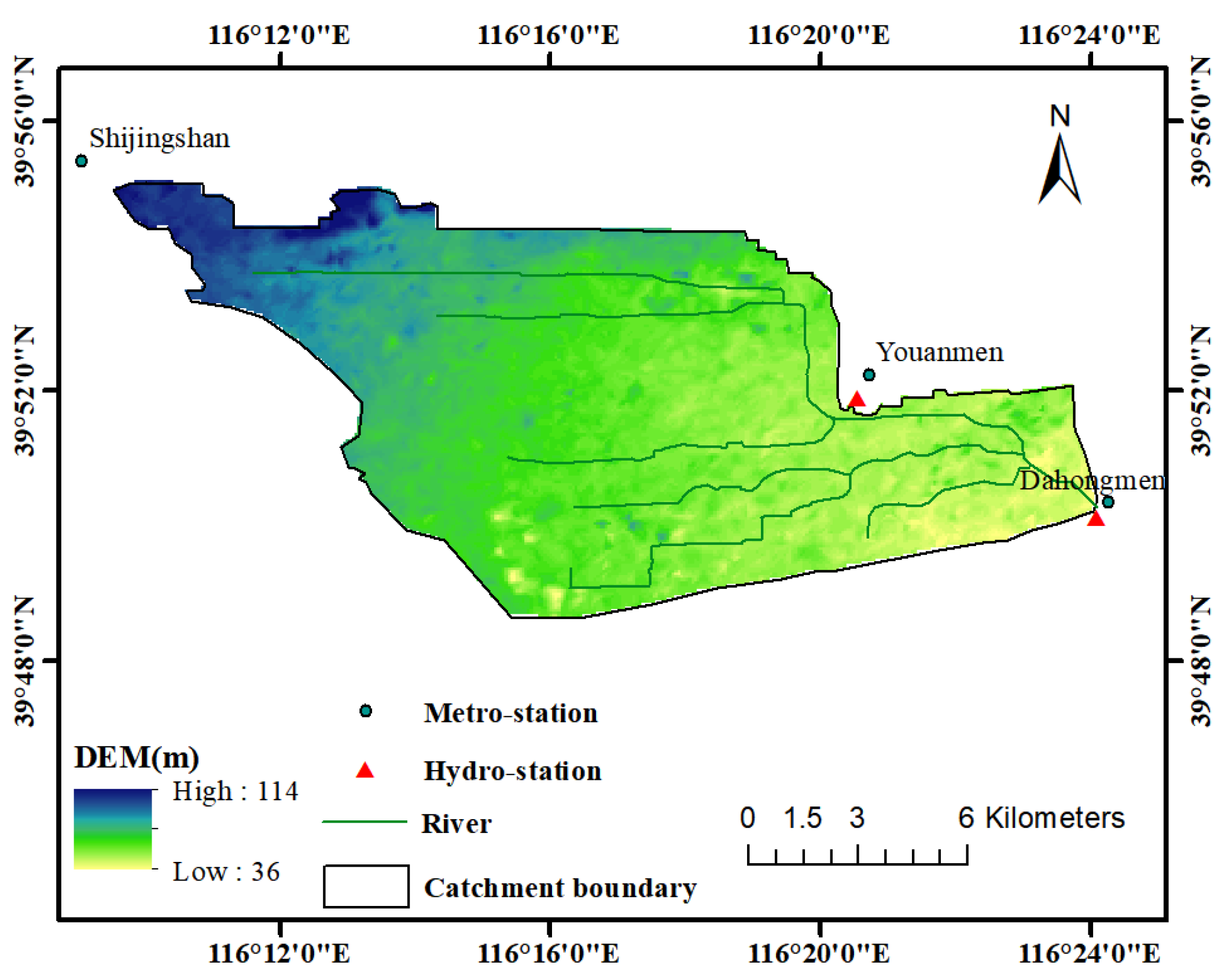
The Dahongmen catchment is a typical urbanized area in Beijing, PRC, with a high population density and heavily built-up underlying surface. The catchment covers an area of approximately 131.49 km2 and is located upstream of the Liangshui River basin in Beijing, between 39°48’–39°55’ N and 116°90’–116°24’ E. In the catchment, the terrain exhibits a downward trend from the western mountains to the eastern plains. The annual average precipitation is 522.4 mm, and 80% of the precipitation occurs during the period from June to September. The river systems and hydro-meteorological stations of the Dahongmen catchment are shown in Figure 1.
3.2. SWMM Model
The SWMM is a dynamic hydrological simulation model used in single-event or long-term (continuous) simulations of runoff quantity and quality from primarily urban areas. The runoff component of SWMM operates on a collection of subcatchment areas that receive precipitation and generate runoff and pollutant loads. The routing portion of the SWMM transports this runoff through a system of pipes, channels, storage/treatment devices, pumps, and regulators [38,39]. Additionally, the SWMM tracks the quantity and quality of the runoff generated within each subcatchment, and the flow rate, flow depth, and quality of the water in each pipe and channel during a simulation period with multiple time steps. In this study, SWMM version 5.1 was used; its technical details have been reported by Rossman et al. [40]. The best performance of SWMM before and after urbanization in the Dahonmen catchment was addressed by Xu and Zhao (2017) [41].
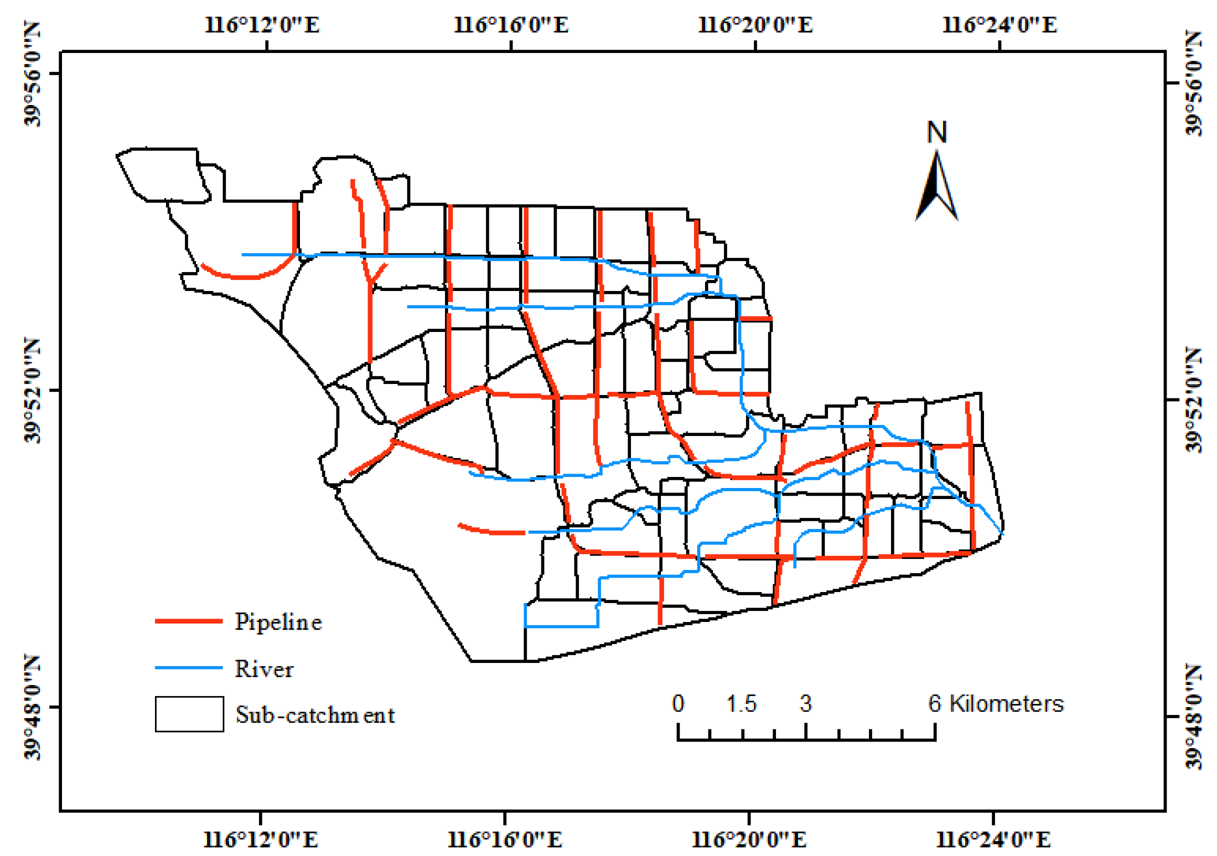
In this study, five heavy storms (accumulated precipitation > 50 mm) occurred between 2011 and 2012 in the Dahongmen catchment were used for model calibration and verification. Precipitation on 23 June 2011, 26 July 2011, and 14 August 2011 were used to calibrate the model, and the other two on 24 June 2012 and 21 July 2012 were used for validation. The accumulated precipitation of the five events was 110.6, 66.8, 66.9, 63.9, and 197.4 mm, respectively. The rainfall duration of the five storms was14, 5, 3, 16, and 18 h, respectively. As shown in Figure 1, the hourly series from three precipitation stations and a DHM gauge station were obtained from the Hydrographic Station of Beijing, CHINA. The hourly inflow data of the Youanmen station were obtained from the Liangshui River Basin Authority. The floodwater from this gate only account for very small amount of streamflow thus will not have great impact on the results of uncertainly analysis. The Digital Elevation Model (DEM) and sewer system map were provided by the National Aeronautics and Space Administration (NASA, ASTER GDEM) and Beijing Municipal Institute of City Planning and Design. These datasets include the locations, section shapes, and conveyance capacities of the river and sewer system in the study area. The catchment was divided into 13 subcatchments, jointly controlled by the river and pipe network, wherein there existed a total of 351 drainage channels (282 watercourses and 69 road drainage channels), as shown in Figure 2.
Table 1 lists the parameters used in the uncertainty analysis of this study, along with their units and distribution. The minimum and maximum values were obtained from the SWMM user’s manual [40] and relevant literature [42,43]. The values for the selected model parameters were randomly selected from uniform probability distributions.
3.3. Interval Evaluation Index
To analyze the effectiveness of the range of uncertainty, we selected three evaluation indices, namely, the average band width (B), coverage (CR), and average relative deviation (RD) [41,44], which are defined as follows:
Here, and are the upper and lower boundary values of the confidence interval; is the observed flow; and is the number of observed values in the confidence interval.
4. Results
4.1. Comparison of Different Acceptability Thresholds
By the application of Monte Carlo method, 10,000 parameter sets were generated within the ranges listed in Table 1. The four objective criteria illustrated in Equations (1)–(4) were calculated by running the SWMM with these sampled parameter sets.
We set the threshold of each objective criterion according to the catchment characteristics and time scale, which are list in Table 2. The number of parameter sets which met the threshold requirements are also list in the table.
As shown in Table 2, 2506 parameter sets could satisfy the requirement of NSE threshold, which is the least in the 4 criteria and indicates NSE is the strictest criterion among them. Nevertheless, R threshold is the most flexible one, 6918 parameter sets can satisfy the criterion. Additionally, all parameter sets that satisfied other criteria thresholds can satisfy R threshold simultaneously.
From Table 2 we can also observe that the number of behavioral parameter sets decreased when more criteria were considered. There are 2226 parameter sets that satisfied the NSE and VB thresholds simultaneously, and 1772 parameter sets that satisfied the NSE and PB thresholds. When we considered all criteria thresholds in GLUE-TOPSIS, the number of behavioral parameter sets reduced to 1598 finally.
4.2. Comparison of Posterior Distribution
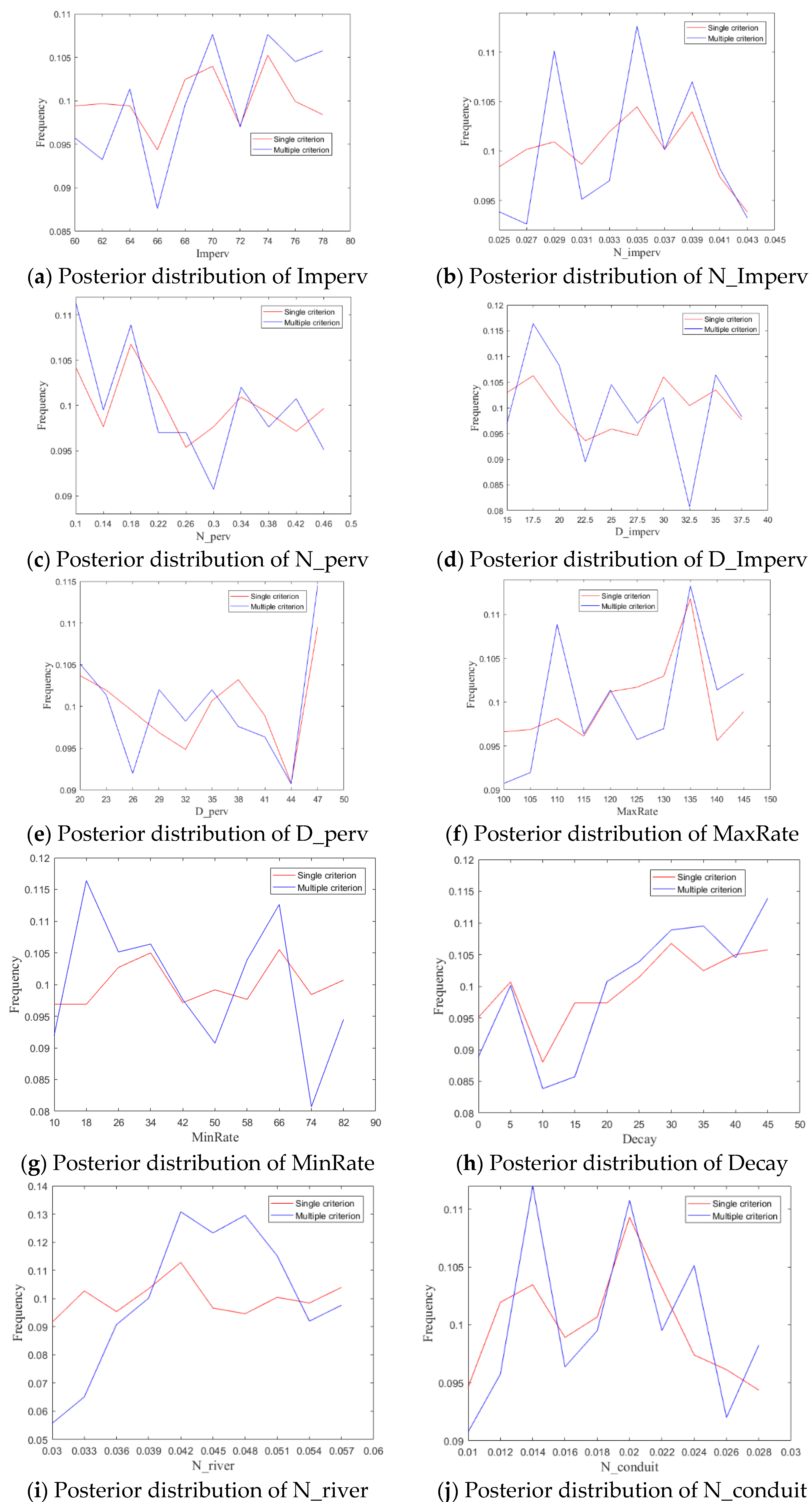
We can obtain the posterior probability distributions of the SWMM parameters from the behavioral parameter sets listed in Table 2. The posterior probability distributions from the single criterion (NSE) and GLUE-TOPSIS are shown in Figure 3.
Obvious difference can be observed between the posterior probability distributions from single criterion (NSE) and those from GLUE-TOPSIS. In general, we can find the obvious areas with high frequency distributions in the posterior probability distribution curves from GLUE-TOPSIS. However, those from single criterion (NSE) are relative flat.
Overall, the posterior probability distributions of Imperv, N-perv, D-perv, MaxRate, Decay, and N-conduit are similar for the two methods. Nevertheless, N-imperv, D-imperv, MinRate, and N-river exhibit a significantly higher frequency interval under GLUE-TOPSIS conditions, which results in higher sensitivity. Notably, there are obvious high-frequency intervals in the parameters characterizing the impervious area, owing to the large impervious area in the DHM catchments. Additionally, the parameter spatial distribution has more than one high frequency interval, which may reflect the “equifinality” of parameter sets proposed by Beven and Binley [25].
4.3. Uncertainty Estimation of Discharge Simulation
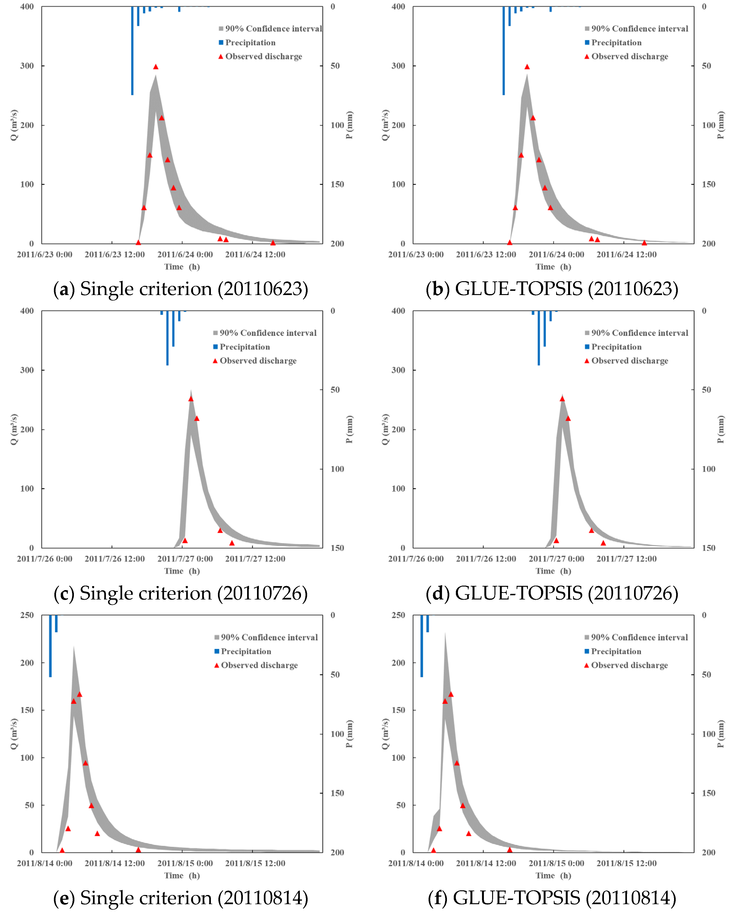
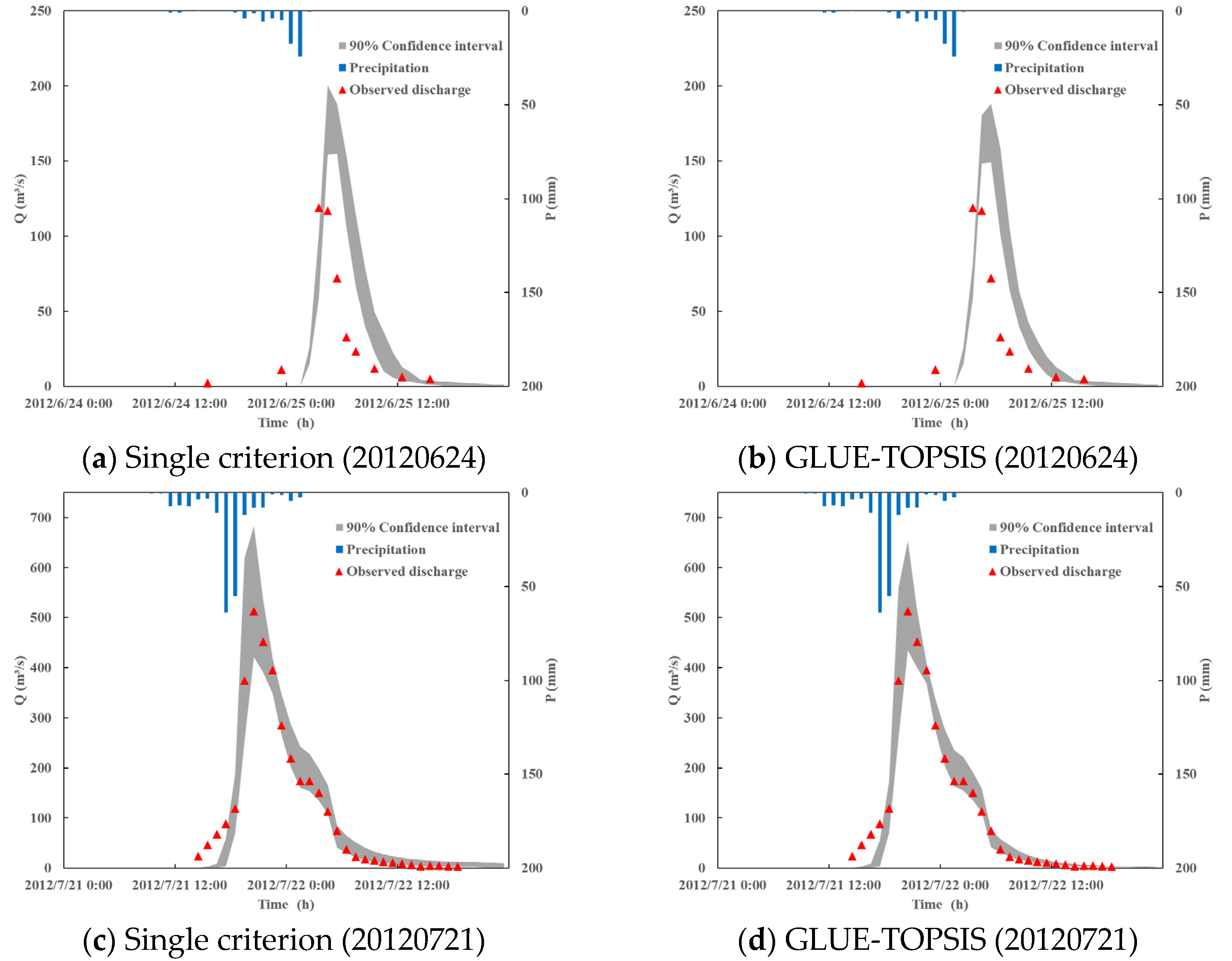
We simulated the SWMM discharge with parameter sets from the single-criterion and GLUE-TOPSIS method. The normalized simulations were sorted by the likelihood value to determine the 95% and 5% uncertainty bounds (90 confidence interval). Figure 4 and Figure 5 present the plotted simulation results obtained by the single criterion and GLUE-TOPSIS methods for five rainfall events during the calibration and validation periods. To analyze the effectiveness of the uncertainty ranges, the evaluation results of the uncertainty indices under the two methods are listed in Table 3.
As shown in Figure 4 and Figure 5, the widths of the uncertainty bound from GLUE-TOPSIS method obviously narrower than those from single criterion method, particularly for the flood peak area and drop section of the discharge curve. Most of the observations fell within the 90% confidence interval, except rainstorm 20120624, which is the smallest storm and may influenced by the strobe operation. However, SWMM model show high performance in rainstorm 20120721, which is one of the most disastrous rainstorms in history.
As presented in Table 3, the band width (B), coverage (CR), and relative deviation (RD) were 46.233, 41.5%, and 24.685, respectively, for single criterion method in the calibration period, and 38.934, 52.3%, and 23.211, respectively, for GLUE-TOPSIS method. In the verification period, B, CR, and RD were 35.526, 45.9%, and 17.120, respectively, for the single criterion method, and 27.970, 47.4%, and 13.754, respectively, for GLUE-TOPSIS method. The results indicate that the GLUE-TOPSIS method show superiority in uncertainty bounds assessment over the single criterion methods, with lower values in average band width (B), average relative deviation (RD) and higher values in coverage (CR).
From the simulation results of the median GLUE estimates in Table 4, it can be seen that under the GLUE-TOPSIS method, the simulation results of NSE, VB are significantly improved compared with the single criterion method, although the VB of 20110623 has a slight increase. The median estimates improved, with an increase of the NSE by 1.6% in the calibration period, and by 10.0% in the validation period. However, the cost criteria PB increased by 0.010 during the calibration period, from the perspective of single field precipitation, the PB of the 20110814 precipitation and the 20120624 precipitation have increased, indicating that the flood peak flow simulation effect is poor. And the benefit criteria R decreased by 0.078.
5. Discussion
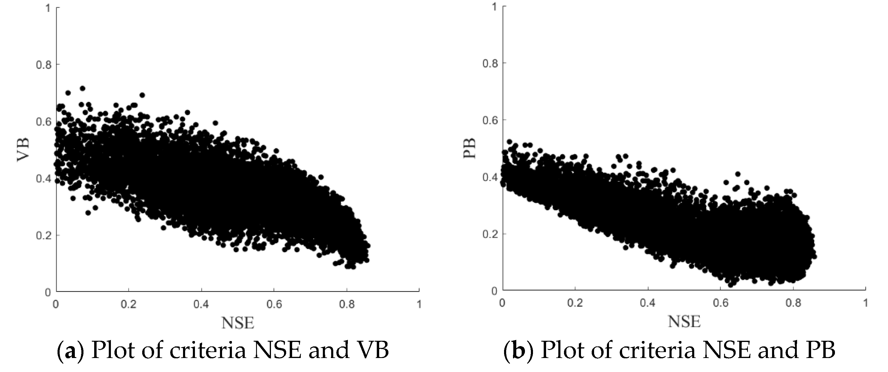
The uncertainties of urban hydrological models have been addressed by several researches [45,46,47,48]. Most researches used single objective function such as NSE or VB as evaluation index [45,46]. As shown in the Figure 6a,b, we found that VB and PB still involved large uncertainties when the NSE was higher than 0.8. This means that a high NSE value can still lead to the poor simulation of the flow volume and flood peak.
Some attempts were made to construct one likelihood function [47,49] considering different objectives. This likelihood function will not work when the objective change. Other important objectives such as overflow and flow in sewer system should be considered in uncertainty analysis of urban hydrological model [15]. The proposed method avoids the process of function construction and is feasible to be applied considering different objectives.
Considering the completeness and consistent of data, five heavy storms between 2011 to 2012 were selected for uncertainty analysis. These are representative enough to test the model reliability for heavy storms. However, small storms are easily affected by local Blue-Green Infrastructure in urban areas that make it difficult to predict [50,51]. Further work needs to test the reliability of the propose method for different magnitude of flood.
6. Conclusions
Urban hydrological models are extensively used in flood forecasting, sponge cities design, and pollution management, etc. The uncertainty assessment of an urban hydrological model is important when evaluating the model’s reliability. Because of the various applications of urban hydrological models, a single criterion is hard to evaluate their performance. In this research, we proposed a multiple-criteria uncertainty analysis method, namely GLUE-TOPSIS, and applies it to the uncertainty assessment of SWMM model in Dahongmen catchment, Beijing. Five typical rainstorm events that occurred during 2011–2012 were investigated and used to test the performance of the proposed method. The conclusions can be summarized as follows:
- 10,000 parameter sets generated by the Monte Carlo sampling in GLUE framework revealed that none of the four commonly used objective criteria could fully represent the urban flow process. Notably, the NSE, which is widely used in assessing the performance of hydrological models also cannot describe the flow characteristics alone, which highlights the need for adopting multi-criteria methods.
- The GLUE-TOPSIS method provided more precise uncertainty bounds and median estimates than traditional GLUE method which used NSE as single criterion. The GLUE-TOPSIS method reduced the bandwidth and deviation of the uncertainty bounds with a higher coverage than these from single criterion. The median estimates of GLUE-TOPSIS are also superior to these from single criterion according to the four objective criteria.
- The SWMM model performed well in the flood simulation of Dahongmen catchment in Beijing, PRC. Most observed flows fell within the 90% uncertainty interval, which suggests that the parameter uncertainty analysis has a relatively high contribution toward improving the simulation accuracy of flood prediction. The comparison results for the posterior distribution revealed that the parameters characterizing the impervious area had obvious high frequency intervals, owing to the large impervious area of Dahongmen catchment.
The GLUE-TOPSIS method provide a feasible way to assess the uncertainty of urban hydrological models, which have been used various aspects in urban water resources management. The users can select objective criteria flexibly and combine them in the GLUE-TOPSIS framework according to their actual needs. We will proceed our research and apply GLUE-TOPSIS to a wider area in water resource management.
Author Contributions
Conceptualization, B.P., G.Z. and R.S.; methodology, B.P., D.P. and Z.Z.; validation, S.S.; writing—original draft preparation, B.P. and G.Z.; writing—review and editing, S.S. and G.Z.; visualization, S.S.; supervision, B.P. and G.Z.; project administration, B.P.; funding acquisition, B.P. All authors have read and agreed to the published version of the manuscript.
Funding
This research was funded by three research programs: (1) National Natural Science Funds of China (Grant No. 51879008); (2) China Scholarship Council (Grant No. 201906045024); (3) China Scholarship Council-University of Bristol Joint PhD Scholarships Programme (Grant No. 201700260088)
Acknowledgments
We thank Liwen Bianji, Edanz Editing China (www.liwenbianji.cn/ac), for editing the English text of a draft of this manuscript.
Conflicts of Interest
The authors declare no conflict of interest.
References
- Shukla, S.; Gedam, S. Assessing the impacts of urbanization on hydrological processes in a semi-arid river basin of Maharashtra, India. Modell. Earth Sys. Environ. 2018, 4, 699–728. [Google Scholar] [CrossRef]
- Barbosa, A.E.; Fernandes, J.N.; David, L.M. Key issues for sustainable urban stormwater management. Water Res. 2012, 46, 6787–6798. [Google Scholar] [CrossRef]
- Hapuarachchi, H.A.P.; Wang, Q.J.; Pagano, T.C. A review of advances in flash flood forecasting. Hydrol. Process. 2011, 25, 2771–2784. [Google Scholar] [CrossRef]
- Hallegatte, S.; Green, C.; Nicholls, R.J.; Corfee-Morlot, J. Future flood losses in major coastal cities. Nat. Clim. Chang. 2013, 3, 802–806. [Google Scholar] [CrossRef]
- Suttles, K.M.; Singh, N.K.; Vose, J.M.; Martin, K.L.; Emanuel, R.E.; Coulston, J.W.; Saia, S.M.; Crump, M.T. Assessment of hydrologic vulnerability to urbanization and climate change in a rapidly changing watershed in the Southeast US. Sci. Total Environ. 2018, 645, 806–816. [Google Scholar] [CrossRef]
- Cristiano, E.; Ten Veldhuis, M.; van de Giesen, N. Spatial and temporal variability of rainfall and their effects on hydrological response in urban areas—a review. Hydrol. Earth Syst. Sc. 2017, 21, 3859–3878. [Google Scholar] [CrossRef] [Green Version]
- Cullmann, J.; Krausse, T.; Philipp, A. Enhancing flood forecasting with the help of processed based calibration. Phys. Chem. Earth 2008, 33, 1111–1116. [Google Scholar] [CrossRef]
- Xu, Z. Hydrological Models: Past, present and feature. J. Beijing Normal Univ. Nat. Sci. 2010, 46, 278–289. [Google Scholar]
- Fonseca, A.; Ames, D.P.; Yang, P.; Botelho, C.; Boaventura, R.; Vilar, V. Watershed model parameter estimation and uncertainty in data-limited environments. Environ. Modell. Softw. 2014, 51, 84–93. [Google Scholar] [CrossRef]
- Zahmatkesh, Z.; Karamouz, M.; Nazif, S. Uncertainty based modeling of rainfall-runoff: Combined differential evolution adaptive Metropolis (DREAM) and K-means clustering. Adv. Water Resour. 2015, 83, 405–420. [Google Scholar] [CrossRef]
- Blasone, R.; Vrugt, J.A.; Madsen, H.; Rosbjerg, D.; Robinson, B.A.; Zyvoloski, G.A. Generalized likelihood uncertainty estimation (GLUE) using adaptive Markov chain Monte Carlo sampling. Adv. Water Resour. 2008, 31, 630–648. [Google Scholar] [CrossRef] [Green Version]
- Lindblom, E.; Madsen, H.; Mikkelsen, P.S. Comparative uncertainty analysis of copper loads in stormwater systems using GLUE and grey-box modeling. Water Sci. Technol. 2007, 56, 11–18. [Google Scholar] [CrossRef] [PubMed] [Green Version]
- Liu, Y.R.; Li, Y.P.; Huang, G.H.; Zhang, J.L.; Fan, Y.R. A Bayesian-based multilevel factorial analysis method for analyzing parameter uncertainty of hydrological model. J. Hydrol. 2017, 553, 750–762. [Google Scholar] [CrossRef]
- Beven, K.; Freer, J. Equifinality, data assimilation, and uncertainty estimation in mechanistic modelling of complex environmental systems using the GLUE methodology. J. Hydrol. 2001, 249, 11–29. [Google Scholar] [CrossRef]
- Thorndahl, S.; Beven, K.J.; Jensen, J.B.; Schaarup-Jensen, K. Event based uncertainty assessment in urban drainage modelling, applying the GLUE methodology. J. Hydrol. 2008, 357, 421–437. [Google Scholar] [CrossRef] [Green Version]
- Setegn, S.G.; Srinivasan, R.; Melesse, A.M.; Dargahi, B. SWAT model application and prediction uncertainty analysis in the Lake Tana Basin, Ethiopia. Hydrol. Process. 2010, 24, 357–367. [Google Scholar] [CrossRef]
- Gupta, H.V.; Kling, H.; Yilmaz, K.K.; Martinez, G.F. Decomposition of the mean squared error and NSE performance criteria: Implications for improving hydrological modelling. J. Hydrol. 2009, 377, 80–91. [Google Scholar] [CrossRef] [Green Version]
- Gupta, H.V.; Sorooshian, S.; Yapo, P.O. Toward improved calibration of hydrologic models: Multiple and noncommensurable measures of information. Water Resour. Res. 1998, 34, 751–763. [Google Scholar] [CrossRef]
- Madsen, H. Automatic Calibration of a Conceptual Rainfall-Runoff Model Using Multiple Objectives. J. Hydrol. 2000, 235, 276–288. [Google Scholar] [CrossRef]
- Fenicia, F.; Savenije, H.H.G.; Matgen, P.; Pfister, L. A comparison of alternative multiobjective calibration strategies for hydrological modeling. Water Resour. Res. 2007, 43, 93–99. [Google Scholar] [CrossRef]
- Gill, M.K.; Kaheil, Y.H.; Khalil, A.; Mckee, M.; Bastidas, L. Multiobjective particle swarm optimization for parameter estimation in hydrology. Water Resour. Res. 2006, 42, 257–271. [Google Scholar] [CrossRef] [Green Version]
- Beven, K.; Binley, A. GLUE: 20 years on. Hydrol. Process. 2014, 28, 5897–5918. [Google Scholar] [CrossRef] [Green Version]
- Hwang, C.L.; Lai, Y.J.; Liu, T.Y. A new approach for multiple-objective decision-making. Comput. Oper. Res. 1993, 20, 889–899. [Google Scholar] [CrossRef]
- Hwang, C.; Yoon, K. Methods for Multiple Attribute Decision Making, 3rd ed.; Springer: Berlin/Heidelberg, Germany, 1981; pp. 58–191. [Google Scholar]
- Beven, K.; Binley, A. The future of distribute models-model calibration and uncertainty prediction. Hydrol. Process. 1992, 6, 279–298. [Google Scholar] [CrossRef]
- Mantovan, P.; Todini, E. Hydrological forecasting uncertainty assessment: Incoherence of the GLUE methodology. J. Hydrol. 2006, 330, 368–381. [Google Scholar] [CrossRef]
- Stedinger, J.R.; Vogel, R.M.; Lee, S.U.; Batchelder, R. Appraisal of the Generalized Likelihood Uncertainty Estimation (GLUE) Method. Water Resour. Res. 2009, 42. [Google Scholar] [CrossRef]
- Clark, M.P.; Kavetski, D.; Fenicia, F. Pursuing the method of multiple working hypotheses for hydrological modeling. Water Resour. Res. 2011, 47, 178–187. [Google Scholar] [CrossRef] [Green Version]
- Freer, J.; Beven, K.; Ambroise, B. Bayesian Estimation of Uncertainty in Runoff Prediction and the Value of Data: An Application of the GLUE Approach. Water Resour. Res. 1996, 32, 2161–2173. [Google Scholar] [CrossRef]
- Beven, K.; Smith, P.; Freer, J. Comment on “Hydrological forecasting uncertainty assessment: Incoherence of the GLUE methodology” by Pietro Mantovan and Ezio Todini. J. Hydrol. 2007, 338, 315–318. [Google Scholar] [CrossRef]
- Loperfido, J.V.; Noe, G.B.; Jarnagin, S.T.; Hogan, D.M. Effects of distributed and centralized stormwater best management practices and land cover on urban stream hydrology at the catchment scale. J. Hydrol. 2014, 519, 2584–2595. [Google Scholar] [CrossRef]
- Nash, J.E.; Sutcliffe, J.V. River flow forecasting through conceptual models part I—A discussion of principles. J. Hydrol. 1970, 10, 290. [Google Scholar] [CrossRef]
- Pang, B.; Guo, S.; Xiong, L.; Li, C. A nonlinear perturbation model based on artificial neural network. J. Hydrol. 2007, 333, 504–516. [Google Scholar] [CrossRef]
- Moriasi, D.N.; Gitau, M.W.; Pai, N.; Daggupati, P. Hydrologic and water quality models: Performance measures and evaluation criteria. T. Asabe 2015, 58, 1763–1785. [Google Scholar]
- Yilmaz, K.K.; Gupta, H.V.; Wagener, T. A multi-criteria penalty function approach for evaluating a priori model parameter estimates. J. Hydrol. 2015, 525, 165–177. [Google Scholar] [CrossRef]
- Cheng, K.; Lien, Y.; Wu, Y.; Su, Y. On the criteria of model performance evaluation for real-time flood forecasting. Stoch. Env. Res. Risk A. 2017, 31, 1123–1146. [Google Scholar] [CrossRef] [Green Version]
- Zanakis, S.H.; Solomon, A.; Wishart, N.; Dublish, S. Multi-attribute decision making: A simulation comparison of select methods. Eur. J. Oper. Res. 1998, 107, 507–529. [Google Scholar] [CrossRef]
- Zoppou, C. Review of urban storm water models. Environ. Modell. Softw. 2001, 16, 195–231. [Google Scholar] [CrossRef]
- Gironas, J.; Roesner, L.A.; Rossman, L.A.; Davis, J. A new applications manual for the Storm Water Management Model (SWMM). Environ. Modell. Softw. 2010, 25, 813–814. [Google Scholar] [CrossRef]
- Rossman, L.A. Storm Water Management Model User’s Manual, 5th ed.; Environment Protection Agency: Cincinnati, OH, USA, 2005; pp. 125–137. [Google Scholar]
- Xu, Z.; Zhao, G. Impact of urbanization on rainfall-runoff processes: Case study in the Liangshui River Basin in Beijing, China. Proc. Int. Assoc. Hydrol. Sci. 2016, 373, 7–12. [Google Scholar] [CrossRef] [Green Version]
- Zhao, G.; Pang, B.; Xu, Z.; Du, L.; Zhong, Y. Simulation of urban storm an Dahongmen drainage area by SWMM. J. Beijing Normal Univ. Nat. Sci. 2014, 50, 452–455. [Google Scholar]
- Shi, R.; Zhao, G.; Pang, B.; Jinag, Q.; Zhen, T. Uncertainty Analysis of SWMM Model Parameters Based on GLUE Method. J. China Hydrol. 2016, 36, 1–6. [Google Scholar]
- Xiong, L.; Wan, M.; Wei, X.; O’Connor, K.M. Indices for assessing the prediction bounds of hydrological models and application by generalised likelihood uncertainty estimation. Hydrolog. Sci. J. 2009, 54, 852–871. [Google Scholar] [CrossRef] [Green Version]
- Zhao, D.; Chen, J.; Wang, H.; Tong, Q. Application of a Sampling Based on the Combined Objectives of Parameter Identification and Uncertainty Analysis of an Urban Rainfall-Runoff Model. J. Irrig. Drain. Eng. 2013, 139, 66–74. [Google Scholar] [CrossRef]
- Wagner, B.; Reyes-Silva, J.D.; Forster, C.; Benisch, J.; Helm, B.; Krebs, P. Automatic Calibration Approach for Multiple Rain Events in SWMM Using Latin Hypercube Sampling. In Green Energy and Technology; Mannina, G., Ed.; Springer: Cham, Switzerland, 2019; Volume 23, pp. 435–440. [Google Scholar]
- Sun, N.; Hall, M.; Hong, B.; Zhang, L. Impact of SWMM Catchment Discretization: Case Study in Syracuse, New York. J. Hydrol. Eng. 2014, 19, 223–234. [Google Scholar] [CrossRef]
- Zhang, W.; Li, T. The Influence of Objective Function and Acceptability Threshold on Uncertainty Assessment of an Urban Drainage Hydraulic Model with Generalized Likelihood Uncertainty Estimation Methodology. Water Resour. Manag. 2015, 29, 2059–2072. [Google Scholar] [CrossRef]
- Sun, N.; Hong, B.; Hall, M. Assessment of the SWMM model uncertainties within the generalized likelihood uncertainty estimation (GLUE) framework for a high-resolution urban sewershed. Hydrol. Process. 2014, 28, 3018–3034. [Google Scholar] [CrossRef]
- Zhu, Z.; Chen, X. Evaluating the Effects of Low Impact Development Practices on Urban Flooding under Different Rainfall Intensities. Water 2017, 9, 548. [Google Scholar] [CrossRef]
- Elliott, A.H.; Trowsdale, S.A. A review of models for low impact urban stormwater drainage. Environ. Modell. Softw. 2007, 22, 394–405. [Google Scholar] [CrossRef]
Figure 1.
Station distribution at Dahongmen catchment.

Figure 2.
Structure of Storm Water Management Model (SWMM) model in Dahongmen catchment.

Figure 3.
Parameter posterior distribution for single criterion and multiple criteria.

Figure 4.
MCDA analysis results for rainstorm events 20110623, 20110726, and 20110814 in calibration period.
Figure 4.
MCDA analysis results for rainstorm events 20110623, 20110726, and 20110814 in calibration period.

Figure 5.
Multiple-criteria decision analysis (MCDA) analysis results for rainstorm event 20120624, 20120721 in validation period.
Figure 5.
Multiple-criteria decision analysis (MCDA) analysis results for rainstorm event 20120624, 20120721 in validation period.

Figure 6.
Relationship between different criteria.


Table 1.
Distribution of SWMM parameters.
| Category | Parameter | Description | Units | Distribution |
|---|---|---|---|---|
| Basic characteristic | %Imperv | Percent of impervious area | % | 60–80 |
| Manning roughness | N-Imperv | Manning coefficient for impervious area | 0.025–0.045 | |
| N-perv | Manning coefficient for pervious area | 0.1–0.5 | ||
| N-river | Manning coefficient for riverway | 0.03–0.06 | ||
| N-conduit | Manning coefficient for conduit | 0.01–0.03 | ||
| Reservoir in depressions | D-imperv | Depth of depression storage on impervious area | mm | 15–40 |
| D-perv | Depth of depression storage on pervious area | mm | 20–50 | |
| Infiltration parameters | MaxRate | Maximum rate on Horton infiltration curve | mm/h | 100–150 |
| MinRate | Minimum rate on Horton infiltration curve | mm/h | 10–90 | |
| Decay | Decay constant for the Horton infiltration curve | h−1 | 0–50 |
Table 2.
Numbers of behavior parameter sets under different criteria.
| Criterion | Number | Criterion | Number | Criterion | Number | Criterion | Number |
|---|---|---|---|---|---|---|---|
| NSE ≥ 0.7 | 2506 | NSE ≥ 0.7 and VB ≤ 0.3 | 2226 | NSE ≥ 0.7 and VB ≤ 0.3 and PB ≤ 0.2 | 1598 | NSE ≥ 0.7 and VB ≤ 0.3 and PB ≤ 0.2 and R ≥ 0.8 | 1598 |
| VB ≤ 0.3 | 3958 | NSE ≥ 0.7 and PB ≤ 0.2 | 1772 | NSE ≥ 0.7 and VB ≤ 0.3 and R ≥ 0.8 | 2226 | ||
| PB ≤ 0.2 | 4215 | NSE ≥ 0.7 and R ≥ 0.8 | 2506 | NSE ≥ 0.7 and PB ≤ 0.2 and R ≥ 0.8 | 1772 | ||
| R ≥ 0.8 | 6918 | VB ≤ 0.3 and PB ≤ 0.2 | 2557 | VB ≤ 0.3 and PB ≤ 0.2 and R ≥ 0.8 | 2396 | ||
| VB ≤ 0.3 and R ≥ 0.8 | 3413 | ||||||
| PB ≤ 0.2 and R ≥ 0.8 | 3927 |
Table 3.
Uncertainty interval evaluation results.
| Method | Criteria | B(m³/s) | CR (%) | RD (m³/s) | |
|---|---|---|---|---|---|
| Calibration period | 20110623 | Single criteria | 48.308 | 54.5 | 13.606 |
| GLUE-TOPSIS | 35.17 | 54.5 | 12.804 | ||
| 20110726 | Single criteria | 50.563 | 20.0 | 41.454 | |
| GLUE-TOPSIS | 43.723 | 40.0 | 40.551 | ||
| 20110814 | Single criteria | 39.829 | 50.0 | 18.995 | |
| GLUE-TOPSIS | 37.908 | 62.5 | 16.276 | ||
| Average | Single criteria | 46.233 | 41.5 | 24.685 | |
| GLUE-TOPSIS | 38.934 | 52.3 | 23.211 | ||
| Validation period | 20120624 | Single criteria | 17.100 | 10.0 | 17.100 |
| GLUE-TOPSIS | 14.100 | 10.0 | 14.150 | ||
| 20120721 | Single criteria | 53.953 | 81.8 | 17.140 | |
| GLUE-TOPSIS | 41.839 | 84.8 | 13.358 | ||
| Average | Single criteria | 35.526 | 45.9 | 17.120 | |
| GLUE-TOPSIS | 27.970 | 47.4 | 13.754 | ||
Table 4.
Simulation results of the median Generalized Likelihood Uncertainty Estimation (GLUE) estimates.
Table 4.
Simulation results of the median Generalized Likelihood Uncertainty Estimation (GLUE) estimates.
| Method | Criteria | NSE | VB | PB | R | |
|---|---|---|---|---|---|---|
| Calibration period | 20110623 | Single criteria | 0.863 | 0.003 | 0.118 | 0.994 |
| GLUE-TOPSIS | 0.876 | 0.02 | 0.112 | 0.995 | ||
| 20110726 | Single criteria | 0.936 | 0.086 | 0.096 | 0.955 | |
| GLUE-TOPSIS | 0.949 | 0.123 | 0.077 | 0.941 | ||
| 20110814 | Single criteria | 0.966 | 0.184 | 0.085 | 0.962 | |
| GLUE-TOPSIS | 0.982 | 0.103 | 0.138 | 0.991 | ||
| Average | Single criteria | 0.921 | 0.091 | 0.099 | 0.970 | |
| GLUE-TOPSIS | 0.936 | 0.082 | 0.109 | 0.975 | ||
| Validation period | 20120624 | Single criteria | 0.429 | 0.402 | 0.375 | 0.790 |
| GLUE-TOPSIS | 0.530 | 0.300 | 0.428 | 0.663 | ||
| 20120721 | Single criteria | 0.936 | 0.041 | 0.077 | 0.989 | |
| GLUE-TOPSIS | 0.974 | 0.005 | 0.059 | 0.962 | ||
| Average | Single criteria | 0.683 | 0.222 | 0.226 | 0.890 | |
| GLUE-TOPSIS | 0.752 | 0.153 | 0.244 | 0.812 | ||
© 2020 by the authors. Licensee MDPI, Basel, Switzerland. This article is an open access article distributed under the terms and conditions of the Creative Commons Attribution (CC BY) license (http://creativecommons.org/licenses/by/4.0/).
Share and Cite
MDPI and ACS Style
Pang, B.; Shi, S.; Zhao, G.; Shi, R.; Peng, D.; Zhu, Z. Uncertainty Assessment of Urban Hydrological Modelling from a Multiple Objective Perspective. Water 2020, 12, 1393. https://doi.org/10.3390/w12051393
AMA Style
Pang B, Shi S, Zhao G, Shi R, Peng D, Zhu Z. Uncertainty Assessment of Urban Hydrological Modelling from a Multiple Objective Perspective. Water. 2020; 12(5):1393. https://doi.org/10.3390/w12051393
Chicago/Turabian StylePang, Bo, Shulan Shi, Gang Zhao, Rong Shi, Dingzhi Peng, and Zhongfan Zhu. 2020. "Uncertainty Assessment of Urban Hydrological Modelling from a Multiple Objective Perspective" Water 12, no. 5: 1393. https://doi.org/10.3390/w12051393
Note that from the first issue of 2016, this journal uses article numbers instead of page numbers. See further details here.