Article

Validating Dynamically Downscaled Climate Projections for Mountainous Watersheds Using Historical Runoff Data Coupled with the Distributed Hydrologic Soil Vegetation Model (DHSVM)

by
Mohammad M. Hasan
1,*,
Courtenay Strong
2,
Adam K. Kochanski
2,
Steven J. Burian
1 and
Michael E. Barber
1
1
Department of Civil and Environmental Engineering, University of Utah, Salt Lake City, UT 84112, USA
2
Atmospheric Sciences, University of Utah, Salt Lake City, UT 84112, USA
*
Author to whom correspondence should be addressed.
Water 2020, 12(5), 1389; https://doi.org/10.3390/w12051389
Submission received: 30 March 2020 / Revised: 6 May 2020 / Accepted: 12 May 2020 / Published: 14 May 2020
(This article belongs to the Section Hydrology)

Abstract

:
The performance of dynamically downscaled climate fields with respect to observed historical stream runoff has been assessed at basin scale using a physically distributed hydrologic model (DHSVM). The dynamically downscaled climate fields were generated by running the Weather Research & Forecasting (WRF) model at 4-km horizontal resolution with boundary conditions derived from the Climate Forecast System Reanalysis. Six hydrologic models were developed using DHSVM for six mountainous tributary watersheds of the Jordan River basin at hourly time steps and 30-m spatial resolution. The size of the watersheds varies from 19 km2 to 130 km2. The models were calibrated for a 6-year period from water year (WY) 1999–2004, using the observed meteorological data from the nearby Snow Telemetry (SNOTEL) sites of the Natural Resources Conservation Services (NRCS). Calibration results showed a very good fit between simulated and observed streamflow with an average Nash-Sutcliffe Efficiency (NSE) greater than 0.77, and good to very good fits in terms of other statistical parameters like percent bias (PBIAS) and coefficient of determination (R2). A 9-year period (WY 2001–2009) was selected as the historical baseline, and stream discharges for this period were simulated using dynamically downscaled climate fields as input to the calibrated hydrologic models. Historical baseline results showed a satisfactory fit of simulated and observed streamflow with an average NSE greater than 0.45 and a coefficient of determination above 0.50. Using volumetric analysis, it has been found that the total volume of water simulated using downscaled climate projections for the entire historical baseline period for all six watersheds is 4% less than the observed amount representing a very good estimation in terms of percent error volume (PEV). However, in the case of individual watersheds, analysis of total annual water volumes showed that estimated total annual water volumes were higher than the observed for Big Cottonwood, City Creek, Millcreek and lower than the observed total annual volume of water for Little Cottonwood, Red Butte Creek, and Parleys Littledell, demonstrating similar characteristics obtained from the calibration results. Seasonal analysis showed that the models can capture the flow volume observed for Big Cottonwood, City Creek and Red Butte Creek during the peak season, and the models can capture the flow volume observed for all the watershed satisfactorily except Big Cottonwood during the dry season. Study results indicated that the dynamically downscaled climate projections used in this study performed satisfactorily in terms of stream runoff, total flow volume, and seasonal flow analyses based on different statistical tests, and can satisfactorily capture flow patterns and flow volume for most of the watersheds considering the uncertainties associated with the study.

1. Introduction

Mountains ensure the availability of water even during off-peak seasons by storing water both in solid and liquid phases and releasing it to streams through the process of runoff. Many mountainous regions generate more than half the total annual runoff of the entire watershed and thus play a dominant role in terms of water availability [1]. Effects of climate change on the hydrological cycle range from global [2] to local [3] scales and are reflected in hydrological time series such as runoff [4] where significant long-term shifts in the amount and timing of river flows create higher risks of water shortages and floods [5,6]. Both precipitation and temperature can change abruptly over short distances in the mountains due to different exposures to radiation, wind, and altitudinal gradients [7]. Small increases in temperature can have large impacts on snow accumulation as well as on the timing of snow accumulation and melting due to their impacts on evapotranspiration rates [8,9]. Understanding the hydrological processes of mountainous watersheds is essential to predict changes in both streamflow quantity and temporal pattern due to future climate change. Understanding historical trends of both spatial and temporal patterns of mountain precipitation and temperature is critical to manage the limited water resources efficiently for the future [10].
Global atmospheric data having spatial resolutions of tens of kilometers are too coarse to provide reliable estimates when used directly in hydrologic models at basin or watershed scales [11]. Modeling of the hydrologic responses of mountainous regions requires hydro-climatic variables at resolutions of 10 km or less to be able to account for the effect of topography on local climate [12,13,14,15,16]. Therefore, studying climate change impacts at basin/watershed scales for mountainous watersheds requires downscaled global climatic model (GCM) fields for both historic and future scenarios. Downscaling of the GCMs can be done either statistically or dynamically. The efficiency of the statistical downscaling approach is highly dependent on the ground observation data so it is not very effective for the regions with limited data availability [17,18]. On the other hand, the dynamical downscaling approach uses conservation equations of mass, momentum, and energy in the form of a regional climate model (RCM) to spatially and temporally refine historic and future atmospheric conditions. This approach is more effective for high mountain areas with complex topographies and for estimating atmospheric data under limited or no data conditions [19,20,21].
Decision makers have tried to use climate model projections under different climate scenarios to understand their effects on the variability of water resources [22] and to support water management decisions [23,24]. According to several studies [25,26], the problem with this approach is that the global or regional climate predictions may strongly differ from the climatic conditions recorded at local weather stations in the watersheds, thus limiting the use of climate change models for predicting the availability of water resources. Another issue with dynamically downscaled climate projections is that they are validated only against precipitation and/or temperature recorded at the local weather stations, but are not evaluated in terms of the stream runoff, which would require using the climate model output to force a physically-based distributed hydrological model for mountainous watersheds. Therefore, despite the ability of dynamically downscaled climate projection models to refine hydro-climatic variables from coarse spatial scales to fine basin or watershed scales, it is not clear how efficient this approach would be in the context of using these hydro-climatic variables to predict future streamflow.
Dynamically downscaled climate projections are region-specific, therefore, for river basin or watershed scale studies for mountainous watersheds, an implementation of a hydrologic model driven by dynamically downscaled climatic variables is expected to be very effective. Due to inherent errors in the dynamically downscaled climate data, it is important to evaluate the historical performance of a dynamically downscaled climate projection as an input into a hydrological model before using it directly to predict streamflow under future climate. Such an evaluation performed for mountainous regions with respect to historic runoff is essential to ensure an adequate level of accuracy of the forecasted future stream discharges under climate change scenarios and to improve confidence in resultant future water management and planning decisions. The objective of this study is to leverage historical stream runoff data for an entire river basin to evaluate a dynamically downscaled climate data set for the intermountain west of the United States region, by coupling regional climate and physically distributed hydrologic models. This unique study performed for the mountainous watersheds of an entire river basin is intended to assess the usefulness and the level of confidence of the dynamically downscaled climate projections in the context of water resource management decisions in data-limited regions.

2. Methods and Data

2.1. Study Area

The Jordan River basin in Utah, USA is a 137 square mile (355 km2) watershed consisting of a 52 mile (135 km) long urban river connecting Utah Lake to the Great Salt Lake, and mountainous tributaries that are important sources of drinking water supply for the population of the surrounding municipalities. This river basin is highly dependent on the snowpack-supplied water resources generated from the adjacent Wasatch Mountains watersheds. Snowmelt is the source of 72% of total annual water runoff from six mountainous sub-basin watersheds. Furthermore, four of these six watersheds (City Creek, Big Cottonwood, Little Cottonwood, and Parleys Creek) contribute 50–60% of the drinking water supply of Salt Lake City [27,28], while other mountainous watersheds upstream of Utah Lake provide 30%, and 10% comes from groundwater [29]. Consequently, understanding the impacts of climate change on local hydrology is imperative in developing plans for a sustainable future. This study examined the six mountainous watersheds of the Jordan River basin presented in Figure 1, which are located to the eastern side of Salt Lake City. The areas of the watersheds vary from 7 square miles to 50 square miles (19 to 130 km2) with elevations ranging from 8000 feet to 11,500 feet (2438 to 3505 m).

2.2. Dynamically Downscaled Climate Projection and Distributed Hydrologic Model

A dynamically downscaled climate simulation for Utah at 4-km horizontal spatial resolution was performed for a 26-year period using the Weather Research and Forecasting (WRF) model driven by initial and boundary conditions derived from the Climate Forecast System Reanalysis as detailed in Scalzitti et al. [27]. Historical hourly climatic variables produced by WRF were used as input to a physically distributed hydrologic model referred to as Distributed Hydrologic Soil Vegetation Model (DHSVM) [30], which simulated stream runoff for the period of nine water years (WY 2001–WY 2009; 1 October 2000 through 30 September 2009). The projected historical streamflow was then evaluated using the measured Salt Lake City Department of Public Utilities (SLCDPU) streamflow data. The Nash-Sutcliffe Efficiency (NSE), coefficient of determination (R-squared), PBIAS, and percent error volume (PEV) statistical tests were performed to evaluate the performance of the dynamically downscaled climate projection.
Accurate simulation of soil, land cover, and climate change are important criteria to consider in selecting a hydrologic model for future watershed planning [31]. Physical hydrologic models using mass and energy conservation equations have high data requirements but are more accurate in predicting the effects of climate change or disturbances [32] than simplified empirical models with low data requirements. DHSVM, used in this study, is a physically-based distributed hydrologic model that provides a dynamic representation of watershed processes at spatial scales [28] taking into consideration the effect of topography, soil, and vegetation, solving the energy and water balance at each grid cell at each time-step. The hydro-climatic inputs into the models are near-surface meteorology including air temperature, wind speed, humidity, precipitation, as well as incoming short- and long-wave radiation. In DHSVM, land cover and soil properties are assigned in each digital elevation model (DEM) pixel, and the size of each pixel of the model is 30 m by 30 m. In DHSVM, evapotranspiration is calculated using a two-layer canopy representation because snow accumulation and melt are calculated using a two-layer energy balance model. Soil moisture and runoff production are estimated using a multilayer unsaturated soil model and a saturated subsurface flow model [33]. Precipitation is categorized as rain or snow based on threshold air temperature. DHSVM calculates a separate one-dimensional water balance for each pixel. According to the model, when the precipitation rate surpasses the maximum infiltration rate, overland flow occurs. DHSVM interpolates wind speeds across the region if multiple stations are available; otherwise wind speeds remain constant. Solar geometry calculations are used to distribute radiation in DHSVM. The model considers each stream section as a linear reservoir, so DHSVM routes the flow as a channel network, and stream runoff (in terms of volume per time step) is provided as an output.

2.3. Data

DHSVM input data can be classified into two general categories which are surface maps and time series data. Hydro-climatic inputs are represented at the model’s computational time steps by time-series, whereas land surface data are represented by spatial maps. A digital elevation model (DEM) is the fundamental base of DHSVM as it describes the watershed topography at a finer scale and all the distributed parameters depend on it. For this study, 1-arc second (i.e., 30-m) DEMs were acquired from the US Geological Survey National Mapping Program for topographic data of the six analyzed watersheds (Figure 2). The DEMs were reconditioned using two routines in ArcMap 10.4.1 to enforce a linear drainage pattern on the DEM grids, which is required by DHSVM to perform hydrologic simulations. The two ArcMap analyses were used to: (i) fill sinks in the drainage area, if any, using the “Spatial Analyst Tools Hydrology” FILL routine; and (ii) delineate the watershed flow path direction from different grid cells to the outlet using the “Flow Direction” routine under the same section as mentioned in previous step. Travel time from a given pixel to the basin outlet was calculated using slope, flow accumulation and flow path information using different routines in “Spatial Analyst Tools” from ArcMap. A minimum number of contributing pixels has been specified based on which stream channel network was imposed on the DEM. Masks of the studying watersheds were generated using “Extraction by Mask” routine of the “Spatial Analyst Tool”. Masks were also used to ensure that all spatial inputs of the models had the same extent. Finally, the watersheds’ mask rasters were used to extract basin values for every pixel from DEM, land cover, soil depth, and soil map raster inputs. Land surfaces were characterized at the same spatial scale for both soil and vegetation cover. For this study, a soil map was obtained from the STATSGO soil database [34]. Some of the important soil parameters required at each pixel by DHSVM are porosity, field capacity, wilting point, and lateral and vertical hydraulic conductivity. According to STATSGO soil database, the six mountainous watersheds analyzed in this study have 10 different types of soil, but each watershed does not have all those types of soil. For example, Millcreek watershed has four types of soil where gravelly loam is the most dominant one with very cobbly loam and loam soils as moderately dominant. Little Cottonwood watershed has seven different types of soil with silt loam and clay loam as the most dominant types of soil. Although the watersheds are very close to each other geographically, they possess unique geological features that may influence hydrological processes.
For vegetation cover, DHSVM requires characterization of both overstory and understory, with the most critical parameters including leaf area index, height, stomatal resistance, radiation coefficient, and albedo. To distribute the vegetation over the watershed, the dominant vegetation type for each layer is defined. A land cover map was derived from the National Land Cover Database (NLCD) 2011 map [35]. A total of 11 different types of vegetation cover were used in this study including deciduous forest, mixed forest, closed shrub, and coastal conifer. Table 1 shows the different types of soil and vegetation available in these watersheds. Vegetation in this model also includes two layers of root zones. DHSVM classifies each pixel based on dominant soil and vegetation type in that pixel and the value of different soil and vegetation parameters are assessed based on those parameters’ values found in the literature.
For calibration of the models, hourly precipitation and temperature values were collected from six SNOTEL stations located in close proximity to the study’s six watersheds, as well as from the Salt Lake City Airport weather station (Figure 3). Then, using the location of SNOTEL stations, humidity, wind speeds, and dew point temperatures were derived from the National Solar Radiation Database (NSRDB) [36] at the same interval and time period as the precipitation and temperature data.
For the historical baseline scenario, several different locations at different elevations were selected within each of the six watersheds. Locations were selected mainly based on elevation as the temperature, precipitation, as well as the form of precipitation (rain versus snow) strongly depended on elevation. Significant changes in slope and aspect were also been taken into consideration in the process of selecting the locations. The number of locations varied with the size of the watershed to ensure sufficient spatial coverage of the climate data. For Red Butte Creek, two stations were selected, whereas for Big Cottonwood Creek, nine stations were selected. Multiple locations at different elevations were used in the historical baseline scenarios to get a better spatial representation of climatic data throughout the watersheds, which was not possible in the calibration process due to the unavailability of so many weather stations. Dynamically downscaled meteorological parameters required for DHSVM were collected at those locations in each watershed, and meteorological station files in text format for each location were created by organizing those data in a specific order as required by DHSVM.
The daily atmospheric transmittance was calculated using the diurnal temperature range [37]. Incoming longwave and shortwave radiation data were estimated from air temperature, dew point temperature, and transmittance following the method developed by Burman and Pochop [38]. Station precipitation data were distributed using 30 years (1981–2010) of monthly normal precipitation maps from the Parameter-elevation Regressions on Independent Slopes Model (PRISM) project [39]. The relationship between precipitation and elevation is not linear so using a constant lapse rate method like the one used for temperature, particularly for an area with significant variation in elevation, increases uncertainty. Therefore, the PRISM distribution was used in this study to represent the complex spatial relationship between precipitation and location. PRISM was used to ensure the explicit representation of the heterogeneity of precipitation in each pixel and, at the same time, to capture the strong gradients of precipitation with elevation. PRISM also considers the influence of rain shadows, complex terrain, coastal proximity, and other complex factors. Furthermore, PRISM has been thoroughly peer-reviewed and has been widely used in modeling applications [40,41]. In our study, we used 800-m resolution maps of 30-year, monthly normals of precipitation. Historic stream runoff data were collected from SLCDPU for the study areas at daily scales.

2.4. Parameterization

DHSVM soil parameters used in this study were mostly based on the values obtained from the literature, as insufficient observed or measured values were available in Utah. Soil parameters like porosity, field capacity, and wilting point were refined within typical ranges to improve the simulation of streamflow and to adjust soil moisture dynamics (Table 2).
In the case of soil parameterization, high and moderately dominated soil parameters were used to calibrate the model while keeping the other soil type parameters constant. The USDA NRCS STATSGO soil database provided physical soil properties including estimated values of saturated lateral hydraulic conductivity (SLHC) and clay content. SLHC was then estimated based on the weighted average of each layer and refined during calibration. During model calibration, hydraulic conductivity could increase or decrease one order of magnitude to serve the purpose of producing reasonable magnitude and shape of peak flows. Sometimes for the same soil types in different watersheds, the parameter values varied, which can be explained considering the contribution of the macropore flow, which was not explicitly implemented in this version of the model.
Parameter values used to represent vegetation cover were estimated from previous studies [42,43,44,45,46,47,48,49]. Maximum snow interception capacity, which means the maximum amount of snow that can be intercepted due to overstory canopy, was set within the range of 0.10 to 0.30 depending on the type and height of vegetation. Rooting depths of trees were set 0.60 m to 0.85 m meaning constant water content values below these depths and high seasonal variation due to extraction of water by roots at shallower depths. Moisture thresholds of different vegetation were estimated as half of the field capacity for mature trees [50] above which transpiration is not restricted by soil moisture.

2.5. Model Setup and Methods of Statistical Analyses

Six hydrologic models have been developed for six different watersheds using DHSVM at hourly time steps and 30-m spatial resolution. Calibrations of these models were performed using observed historical daily streamflow at the basin outlets. The models required initial conditions of the hydrologic state variables like interception of snow and rain by each vegetation layer, number of root zone layers, and soil moisture content in each soil layer. These initial variables are not easy to estimate so the models were run for a spin-up period of 9 months from 1 January to 30 September with the result not taken into consideration. During the spin-up period, three root zone layers and two vegetation layers were selected as the maximum number of layers, respectively. In addition, soil moisture, soil surface temperature, and soil temperature for each root zone layer were set to default values, and other model state variables were kept at 0. The calibration period was initially chosen from 1 October 1998 to 30 September 2004 to include at least one wet year and one dry year. However, due to the unavailability of observed precipitation and temperature data from the nearest SNOTEL sites, three of the watersheds have different calibration periods. The calibration period for Little Cottonwood and Millcreek watersheds was 1 October 1998 to 30 September 2004, whereas for Parleys Littledell the calibration period it was 1 October 1999 to 30 September 2004, and for Red Butte Creek the calibration period was 1 October 2000 to 30 September 2004. We selected Big Cottonwood and City Creek watersheds to perform both calibration and validation tests for two separate timelines to see whether there is any significant difference between calibration and validation results. Big Cottonwood watershed is calibrated for WY 1999 to WY 2001 and validated for the period of WY 2002 to WY 2004. For City Creek watershed, the calibration and validation period are WY 2001 to WY 2002 and WY 2003 to WY 2004, respectively.
The Nash-Sutcliffe Efficiency (NSE), a statistical test which has been used widely to compare the extent of simulated variance to observed variance [51], was used as the main tool to evaluate the performance of the models. Input parameters were changed within permissible limits to maximize the NSE index between simulated and observed streamflow. The range of NSE value is −∞ to +1, where +1 represents a perfect model. NSE values between 0 and 1 indicate an acceptable level of performance [51,52]. A recent study [53] showed that any NSE ≥ 0.65 indicates an acceptable performance of the hydrologic models, whereas, in past hydrologic modeling studies, values close to 0.4 have been deemed as satisfactory [54,55].
Additional statistical tests involving the coefficient of determination, percent bias, and percent error volume (PEV) were performed to evaluate overall model performance together with NSE. Hourly simulated streamflows were converted to average daily flows using a self-developed R-code using various R-packages before performing any statistical tests mentioned above.
Calibrated hydrologic models of the six study watersheds were used to evaluate the performance of the dynamically downscaled historic climate projection data for the historical baseline of WY 2001 to WY 2009 in terms of stream runoff. DHSVM model requires different meteorological parameters like temperature, humidity, precipitation, wind speed, and solar radiation. As we performed the calibration using the observed meteorological data, the time period for which all those parameters are available for the study areas is WY 1999–2004. The historical baseline period of the dynamically downscaled climate projection is WY 2001–2009. So there is an overlap of some years in between calibration and historical baseline scenario.
Previously, in the calibration phase, the SNOTEL sites closest to the watersheds were used as the sources of climatic input data. For the historical scenario, multiple locations within the watershed were selected (Figure 4) at which the dynamically downscaled historic climate projection for temperature, humidity, precipitation, wind speed, and solar radiation were estimated and then spatially distributed via the variable Cressman (VARCRESS) interpolation method, using one of the three default methods used in DHSVM. The technique, developed by George Cressman [56], interpolates station data to a user-defined latitude-longitude grid. According to this technique, multiple passes are made through the grid at smaller radii of influence, which increases precision. Calibrated models were run for the historical baseline period using these dynamically downscaled hydroclimatic data keeping all other input parameters the same to ensure that the results of the models represent the performance of the dynamically downscaled climate fields.

3. Results and Discussion

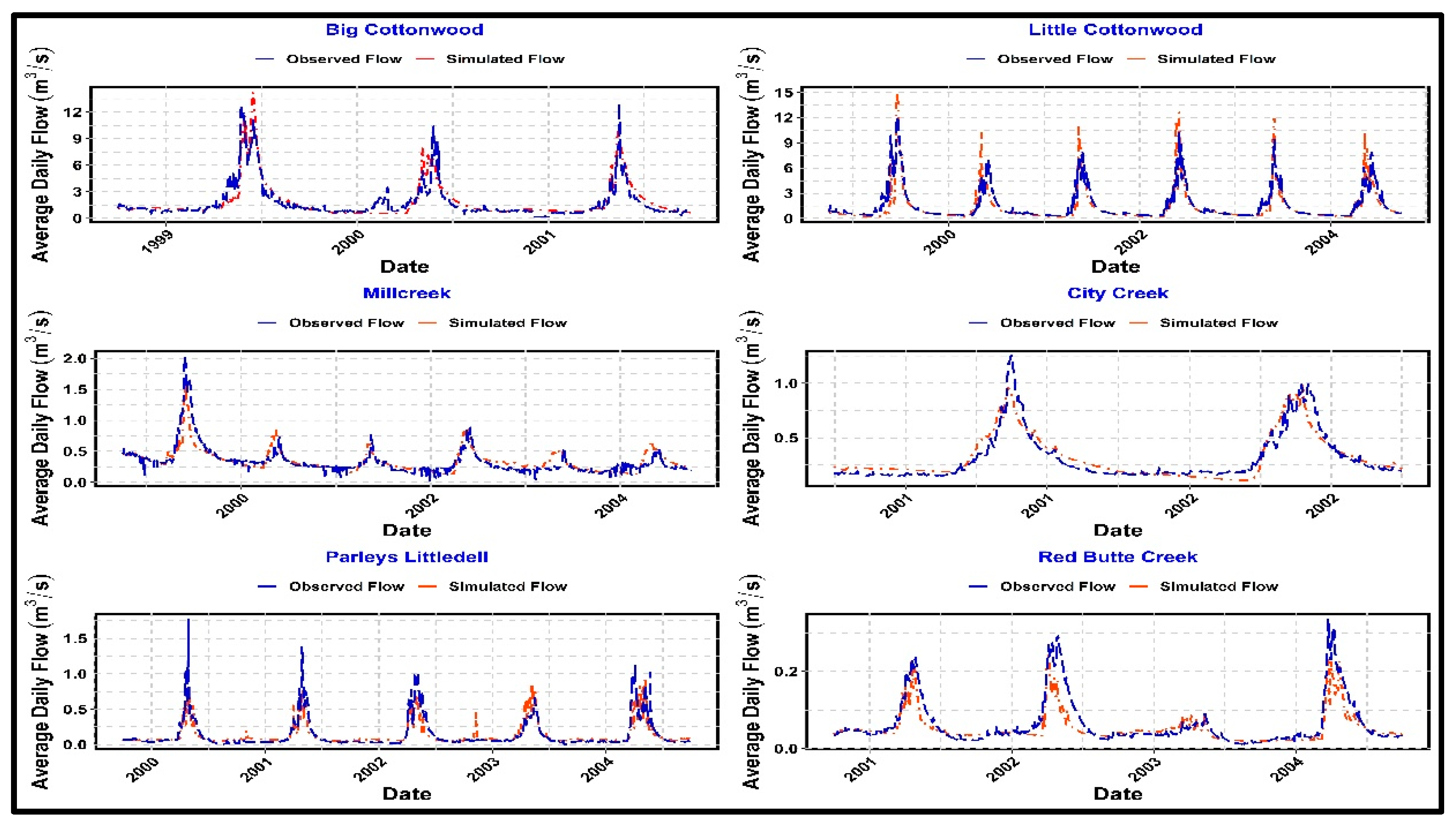
3.1. Calibration and Validation Results

The observed and simulated hydrographs for the calibration period of the hydrologic models of six watersheds are shown in Figure 5. Overall, the model slightly underestimated the peak flows for all the watersheds except Little Cottonwood and estimated reasonably well the dry season base flow in most of the cases.
Results of the statistical tests performed to evaluate the models’ performance are shown in Table 3. The Nash–Sutcliffe efficiency indices of the models were within the range of 0.71 to 0.83 with the lowest (0.71 for Parleys Littledell) indicating a very good to satisfactory fit of simulated and observed streamflow in terms of amount and timing of flows. Similarly, the coefficient of determination (R2) for the models ranges from 0.721 to 0.841, which means the performance rating of developed calibrated hydrologic models for four out of six watersheds were very good while the performance ratings of Little Cottonwood and Red Butte Creek models were good. A percent error volume (PEV) test was also done to understand the models’ performance in terms of estimating the total volume of water for the whole calibration period. From the PEV tests, it was clear that the performance of all the hydrologic models was very good except for Little Cottonwood and Red Butte Creek. The performances of those two models were good. Model results were evaluated using those statistical tests according to general performance ratings for recommended statistics (Table 4) [52].
Calibration results indicate that the developed models were unable to reliably generate flows under specific climatic circumstances like when the streams became frozen and flows due to heavy snow and rain occurred on the same day. The models also struggled to predict small peaks due to small, isolated rainfall events in summer. From the PEV results, it was found that the models for Little Cottonwood, Red Butte Creek, and Parleys Littledell underestimated the total volume of water, whereas the models for Big Cottonwood, Millcreek, and City Creek overestimated the total volume of water over the calibration period.
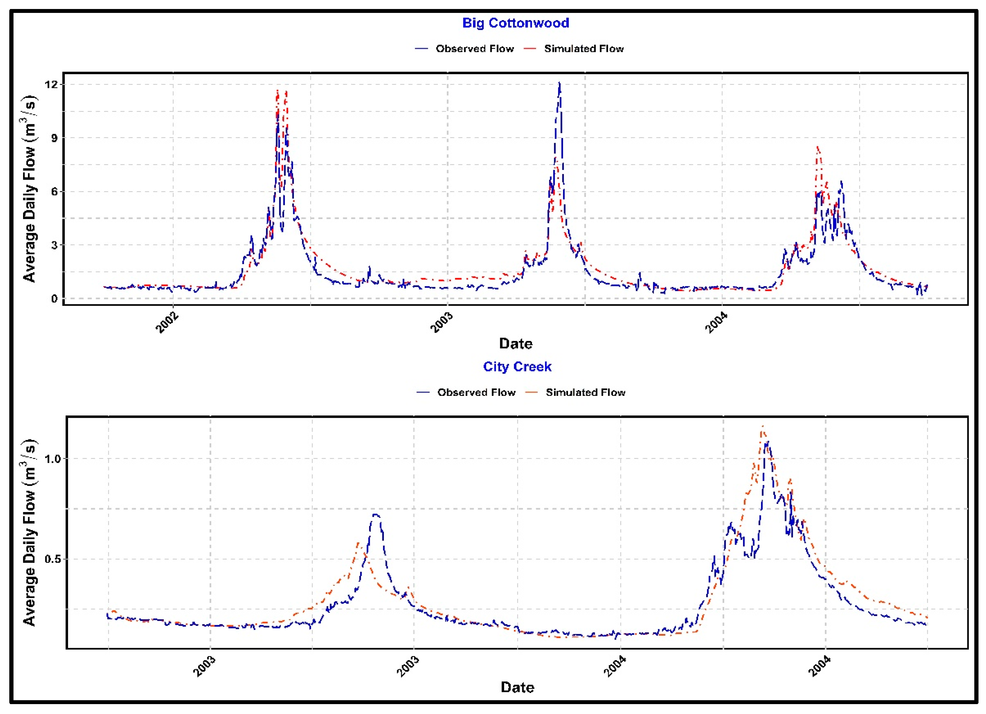
Figure 6 shows the validation results of Big Cottonwood and City Creek. The statistical analyses for the validation run shown in Table 5 do not exhibit any significant difference with the calibration results. The downside of calibrating for shorter periods is that there is greater potential to miss the range of hydrologic variability so the four remaining watersheds used a longer calibration period.

3.2. Historical Baseline Scenario

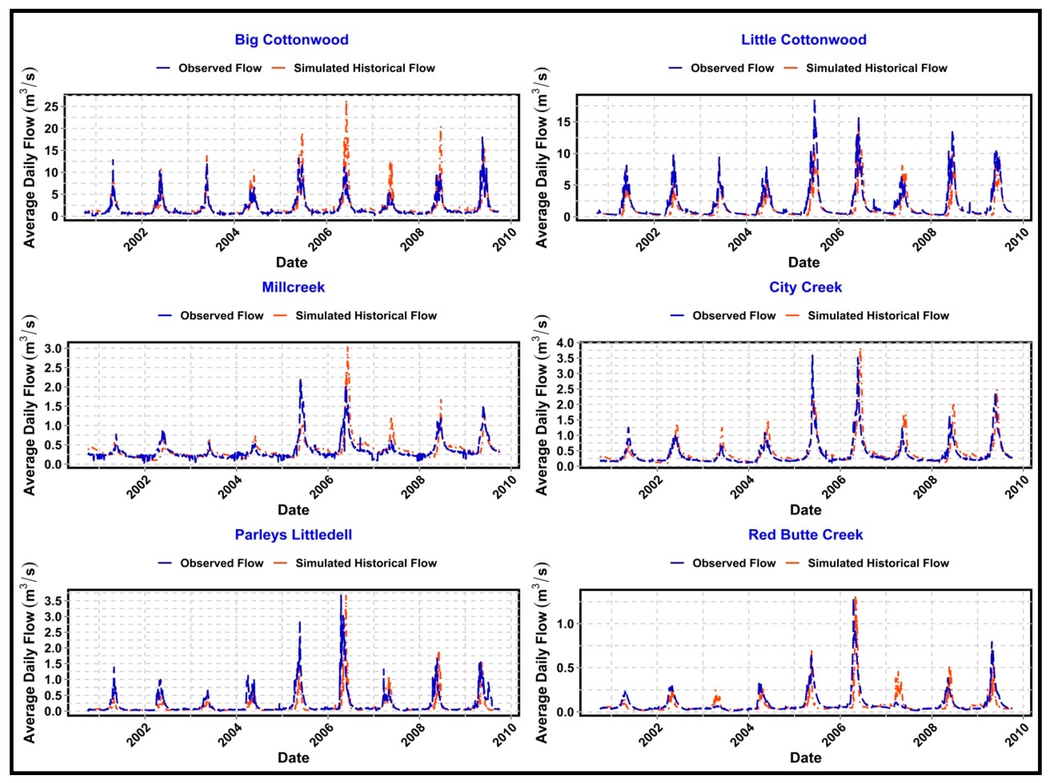
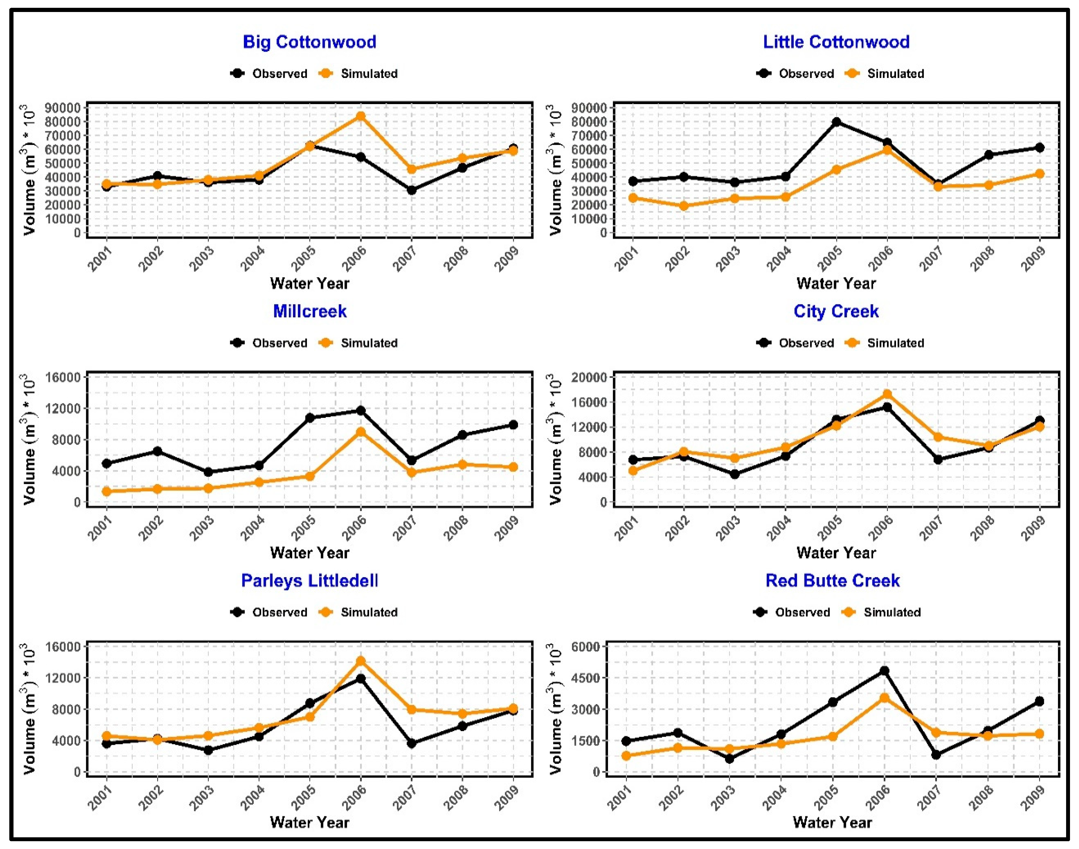
The observed and simulated hydrographs of six watersheds for the historical baseline period are shown in Figure 7. Unlike the calibration period, the model slightly overestimated the peak flows for all the watersheds except for Little Cottonwood and Parleys Littledell and estimated reasonably well the dry season base flow in most of the cases. Although the timing of the simulated peak runoffs were usually delayed compared to the observed peak flows, the base flows during the historical baselines were estimated satisfactorily by the model, which is important for estimating drought impacts on water supply and ecosystem services.
The NSE values comparing observed and simulated stream runoff ranged from 0.41 to 0.72 (Table 6) for the six models. In terms of NSE and R2 values, Little Cottonwood and City Creek watersheds exhibited good and satisfactory fits with the observed flow, respectively. The coefficients of determination ranged from 0.52 to 0.77, with values above 0.50 indicating an acceptable fit between observed and simulated flows (Table 6) for all the watersheds. The NSE and R2 analysis suggests that the model can predict the amount of flow at a satisfactory level for all the watersheds but might not be able to predict the timing of the flow at a satisfactory level for all the watersheds except Little Cottonwood and City Creek.
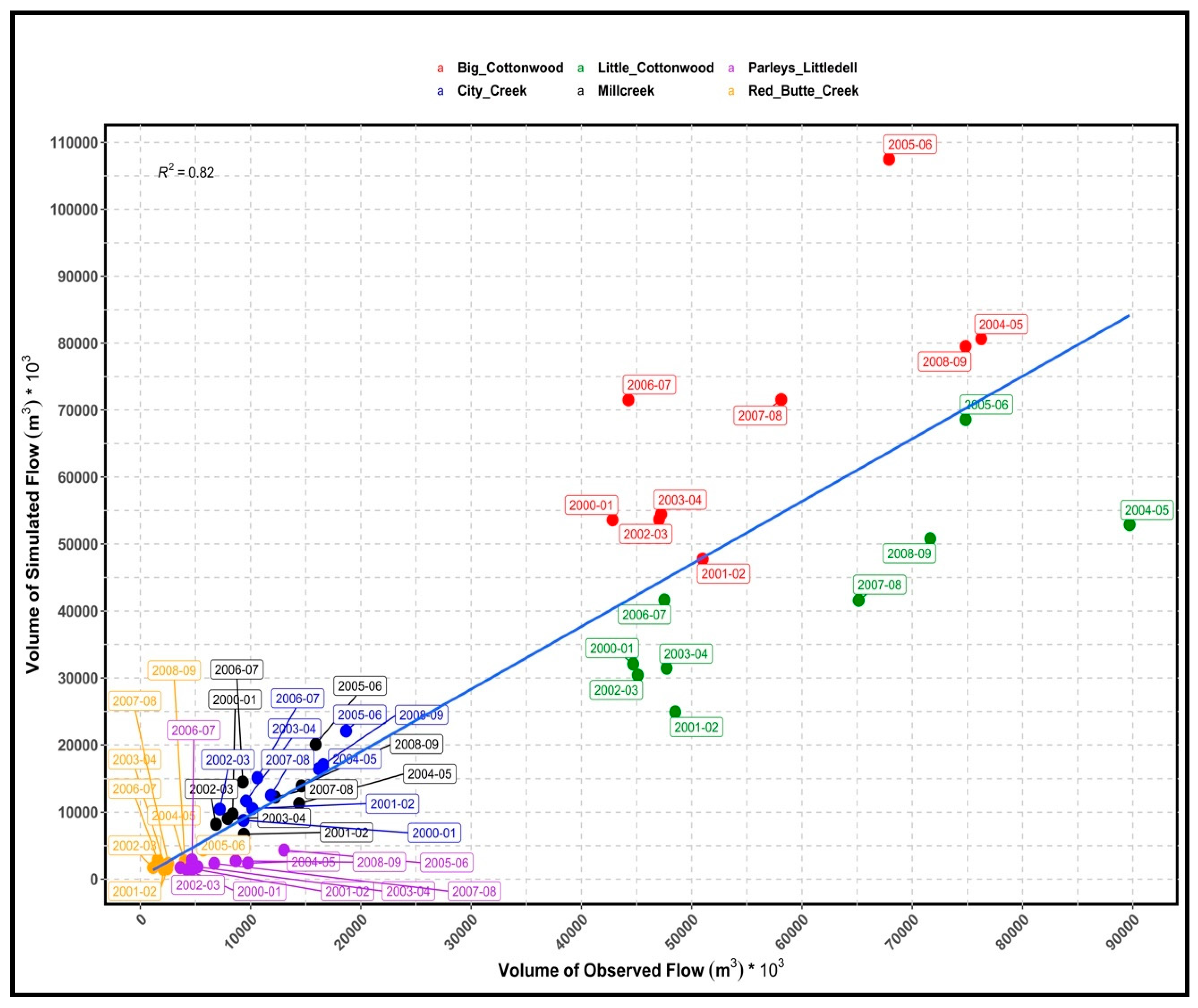
Simulation of flows (peak and base) is conventional for the acceptance of the validity of a model, but for water supply and drought analysis, the available volume is more important and relevant. Moreover, as we wanted to evaluate the performance of the dynamically downscaled climate fields by using them to force a hydrologic model, we also tried to analyze the results of the historical baseline simulation in terms of the total annual volume of flow and seasonal volume of flow. The water year in the USA starts on 1 October and ends on 30 September. For our analysis, we considered March through August of a water year as the peak seasonal flow period and October through February plus September as the dry season flow period. The total annual volume of water analysis (Figure 8) showed that simulated volumes of water were higher than the observed total annual volume of water for Big Cottonwood, City Creek, and Millcreek and lower than the observed volumes of water for Little Cottonwood, Red Butte Creek, and Parleys Littledell. These results were similar to observations found in the calibration results, although the bias in the volume of water was higher. The value of R2 is 0.82, which shows a very good fit between the simulated and the observed annual volume of water taking all the watershed into consideration.
While Figure 8 gives an overall indication of the performance of the historical climate projections based on the simulated and the observed annual volume of water, the statistical analysis shown in Table 7 provides a better representation of the performance of dynamically downscaled climate projections for the individual watersheds. The R2 value of 0.82 and 0.70 show a very good and good fit for City Creek and Parleys Littledell respectively while indicating a satisfactory fit for all the other watersheds. PEV analysis shows a very good fit for Millcreek and good to satisfactory fit for all the other watersheds except Big Cottonwood.
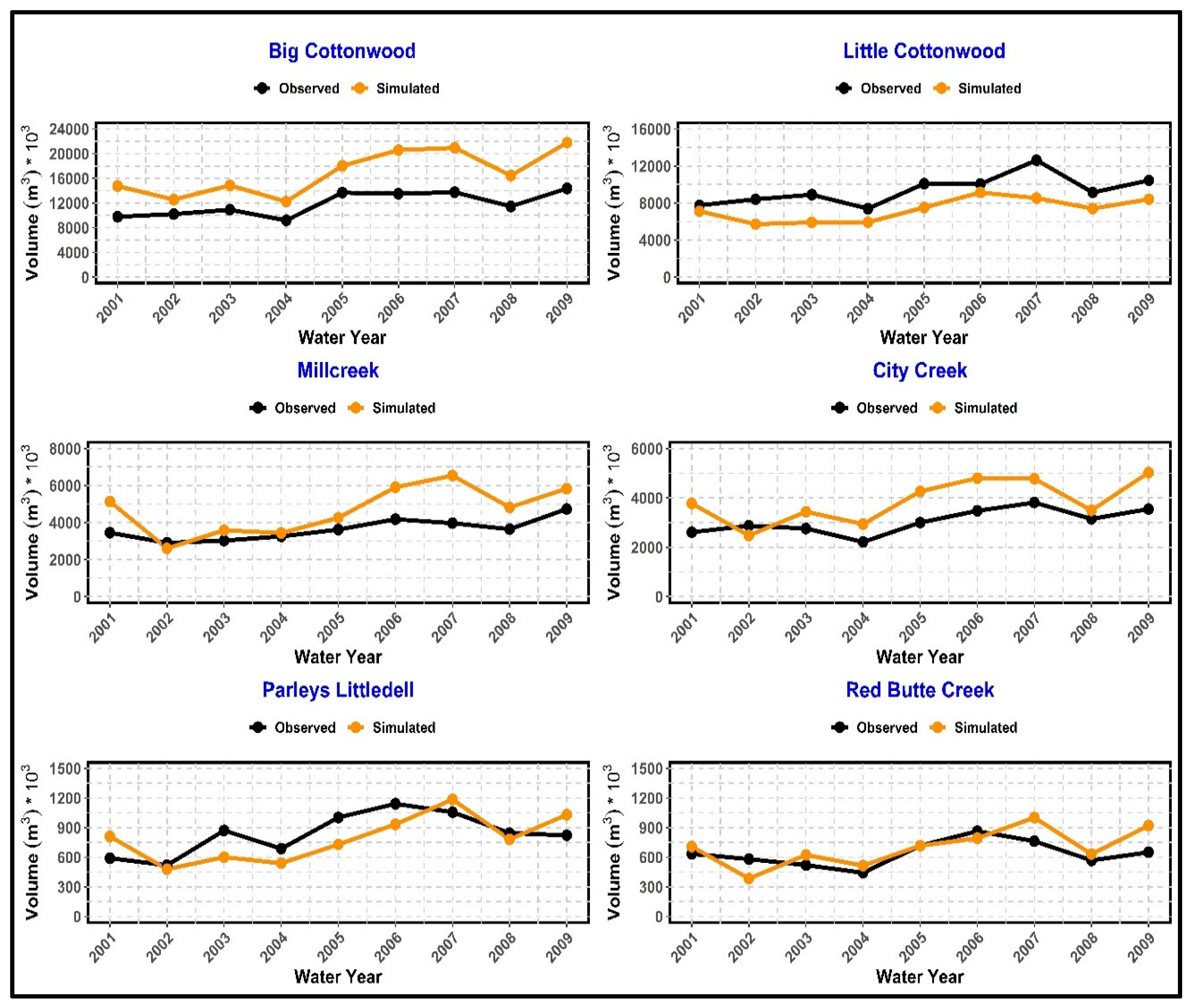
Peak seasonal volume analysis (Figure 9) shows that except for Little Cottonwood and Millcreek watersheds, the simulated volume of peak seasonal flow matched reasonably well with the observed volume for other watersheds (the differences in the smaller watersheds are due to scale). The simulated volume of peak seasonal flow for Little Cottonwood and Millcreek is lower than the volume of observed flow throughout the historical baseline period. In the case of dry season volume analysis (Figure 10), the model matched well with the observed volumes for the smaller watersheds but overestimated for Big Cottonwood, Millcreek, and City Creek while slightly underestimating the volumes for Little Cottonwood and Parleys Littledell watersheds.
Results of the statistical tests performed to evaluate the models’ performance in terms of seasonal flow volume analysis are shown in Table 8. Considering the R2 value, the model simulations of peak and dry season volume varied from satisfactory to very good for all the watersheds. In terms of the PEV analysis, the model simulations are inconclusive although the performance ratings are slightly better for dry season volumes compared to peak seasons’ considering two very good ratings for dry season compared to one for peak season, and the average error is slightly lower in dry season (21% as against about 24%) compared to peak season. From the seasonal volume flow analysis perspective, it can be concluded that the models performed better in estimating dry season flow (considering better R2 values and slightly higher PEV ratings) than the peak season flow. High spatial variability in winter storms (discussed later in the uncertainties section) is a likely cause for peak flow discrepancies. From the seasonal volume analysis perspective, it can be concluded that the models performed better in estimating dry season flow (considering better R2 values and slightly higher PEV ratings) than the peak season flow. High spatial variability in winter storms (discussed later in the uncertainties section) is a likely cause for peak flow discrepancies.
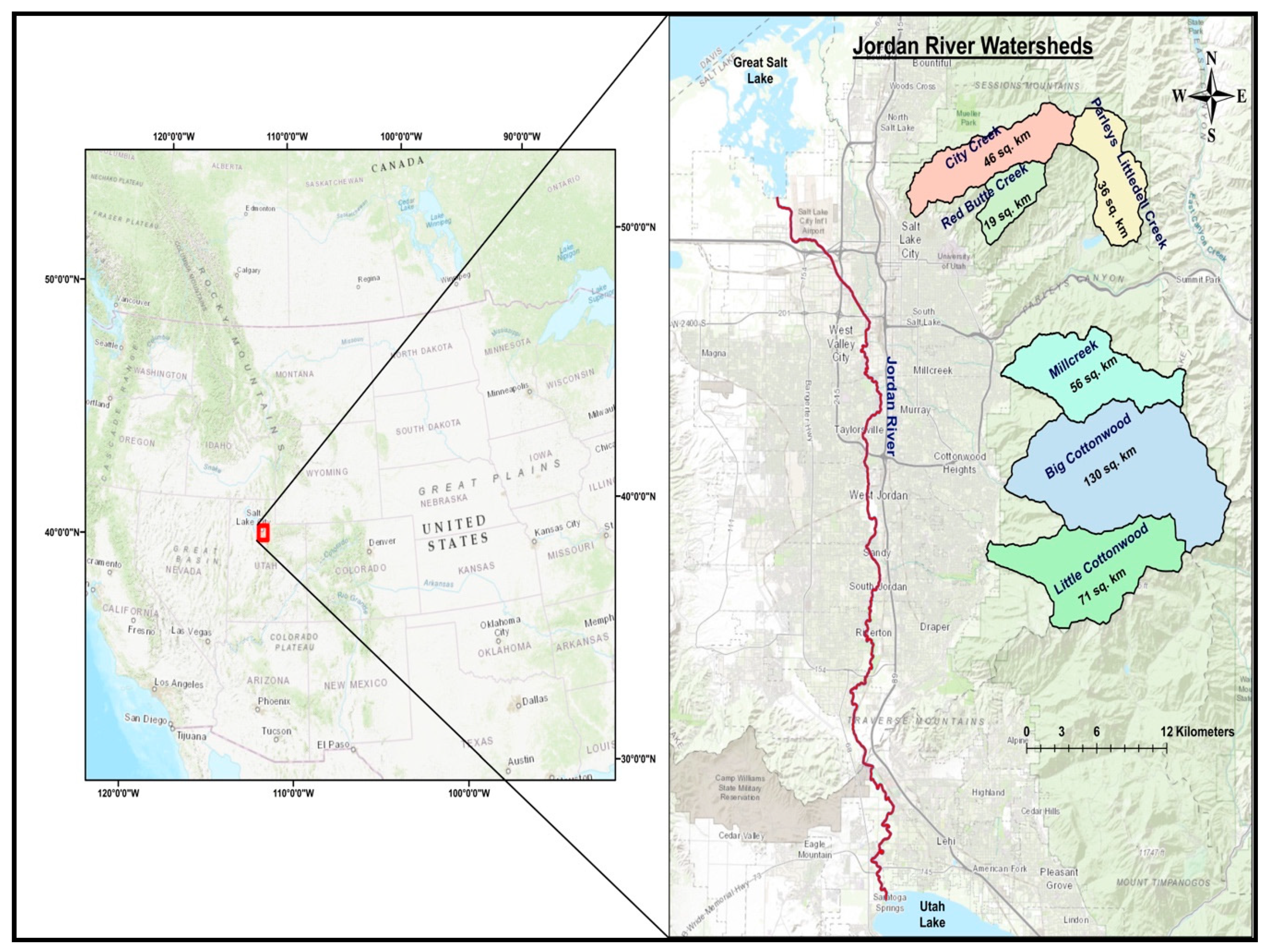
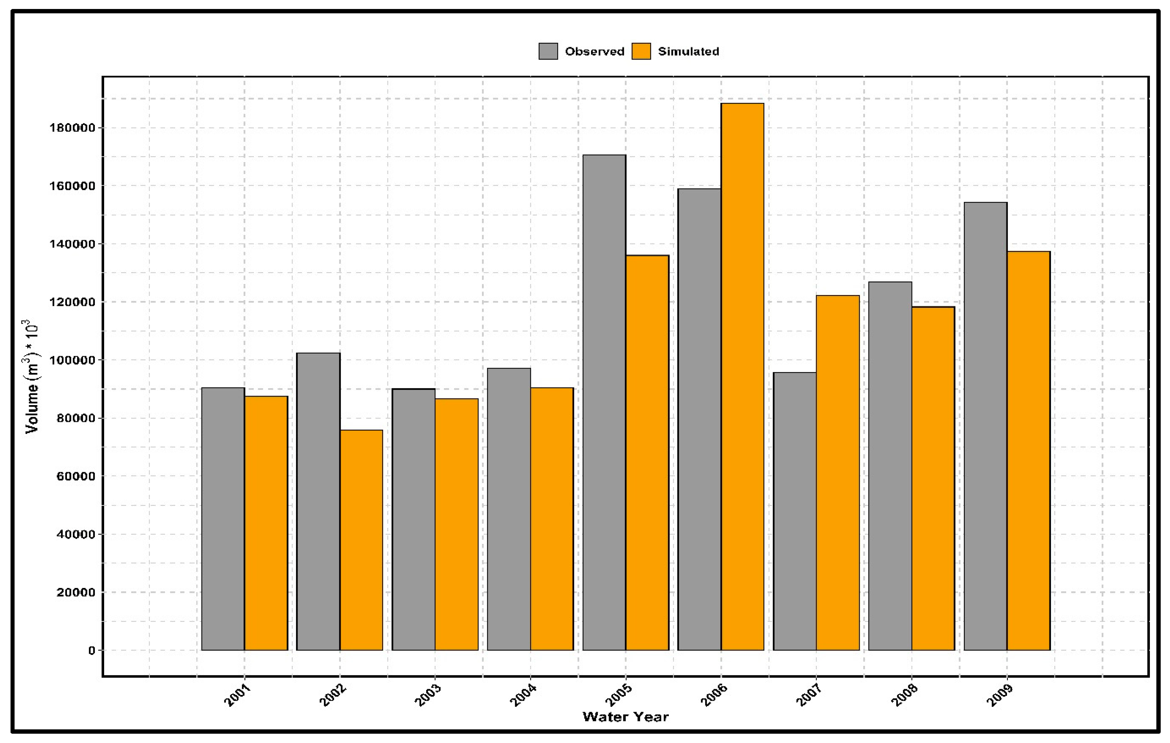
These six watersheds are the major contributors to the Jordan River downstream of Utah Lake and are the primary sources of drinking water for Salt Lake City, so to get a better understanding of how the dynamically downscaled climate projection depicts the downstream drinking water supply, we compared the total volume of simulated flow coming from theses six watersheds to the observed total volume. As presented in Figure 11, the total amount of simulated flow is comparable but slightly lower than the observed flow for all the years except WY 2005–2006 and 2006–2007. Over the 9-year period for the Jordan River basin, the total amount of simulated flow is 4% lower than the total amount of observed flow.
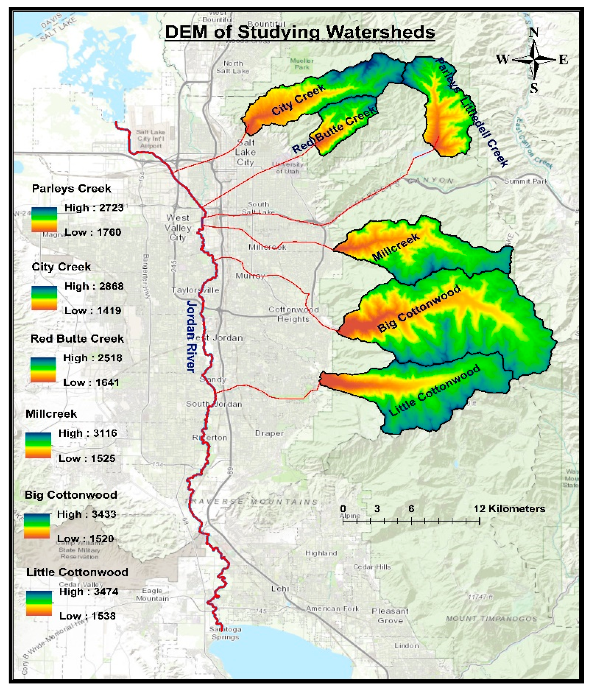
In mountainous watersheds, the form of precipitation and snow melting processes depend strongly on elevation as snowfall increases rapidly with elevation and the melting of snow at the beginning of the season starts at lower elevations [
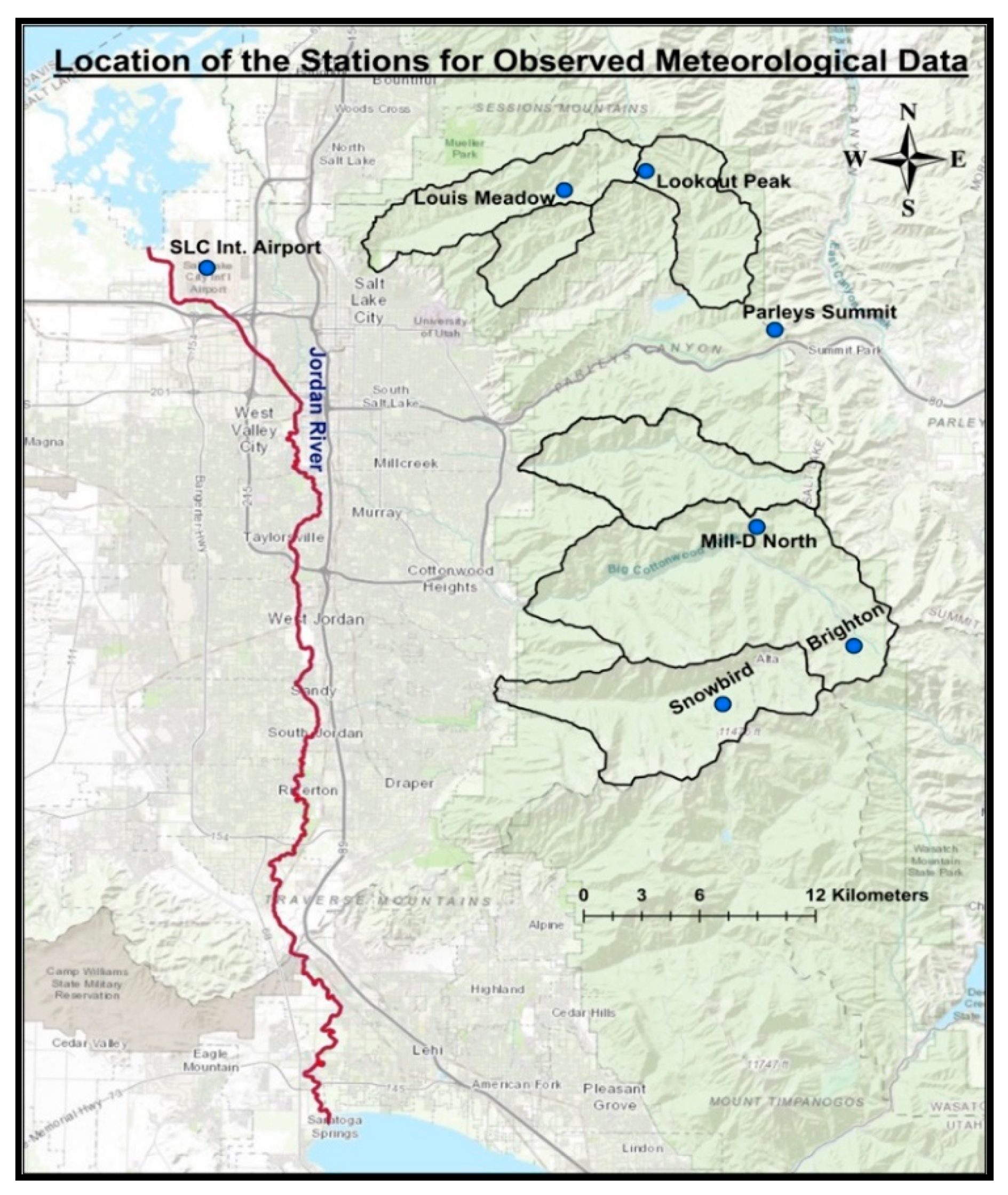
57]. The observed data from the SNOTEL stations did not provide a clear indication about the transformation of a precipitation event from snow to rain or vice versa with the change in elevation. Additional snow stations would help to get a better estimation of the spatial variability of the snow depth.
Although the six watersheds are located adjacent to each other, they are very unique in terms of elevation, slope, aspect, soil types, and vegetation. DHSVM is a physically distributed model so elevation, aspect, and slope were handled quite well. In the case of soil parameters, however, the basin models were predominantly based on values obtained from previous studies and default model values since no watershed-specific measurements of soil depth, hydraulic properties, and soil moisture parameters were found in the literature. The lack of site-specific parameter data likely increases the uncertainty in model results. Soil types vary from bedrock to sandy loam to clay loam or granular silt loam among neighboring watersheds. Furthermore, sometimes the same soil in different watersheds might have different soil properties due to the geographical and overall condition of the watershed. Vegetation parameters like height, root zone depth, and leaf area index (LAI) were derived from the readily available literature and various online databases. The use of generalized values of the input parameters due to lack of region-based observed or measured values could have contributed to lower the model efficiency.
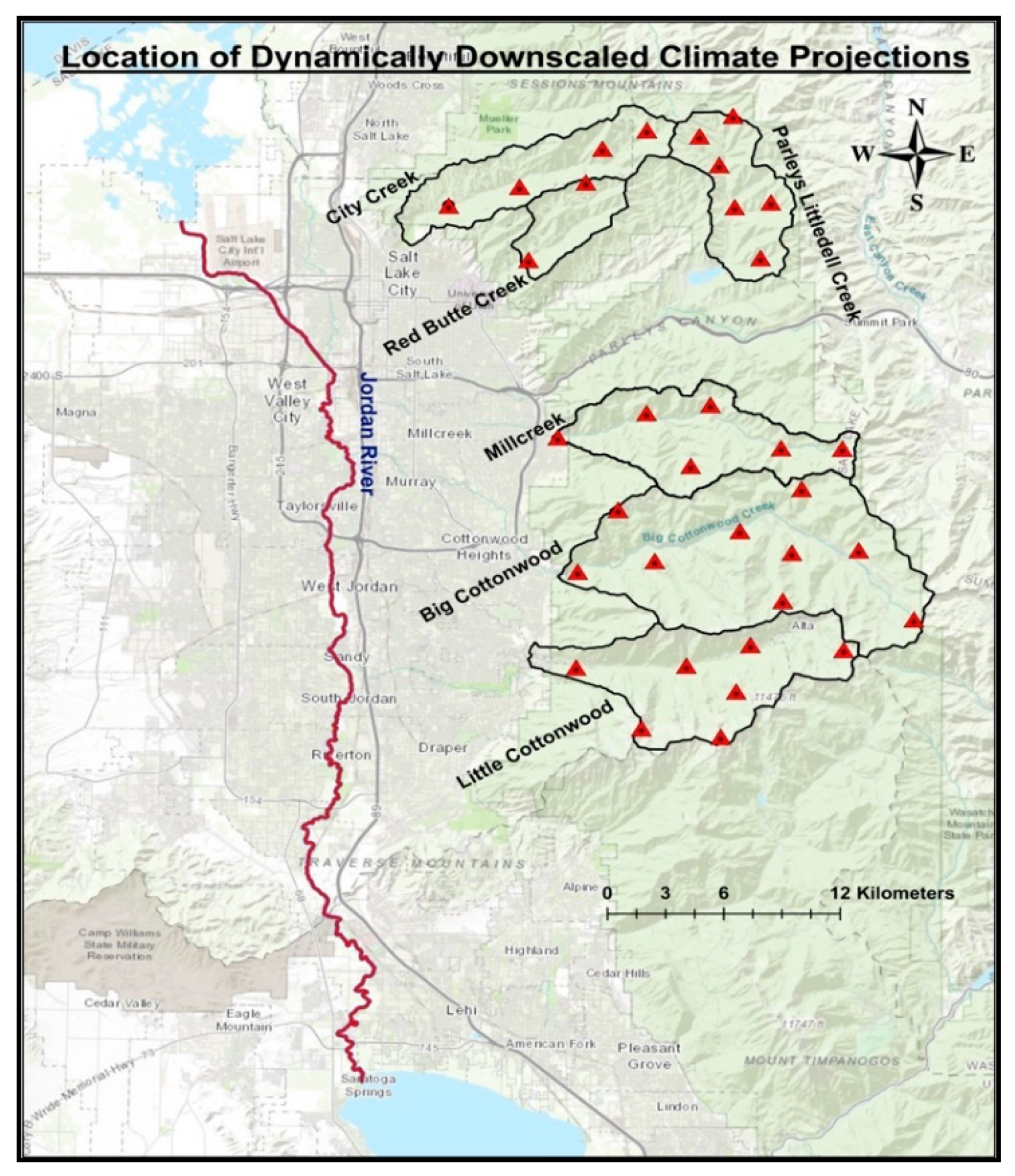
The spatial scale of DHSVM is 30 m, whereas the spatial resolution of the dynamically downscaled climate projection is 4 km. Although fine-scale downscaling of climate predictions from 4 km to 90 m has been done in some areas for temperature and precipitation [58], the process characteristics and data sets required to reduce downscaling uncertainties in most mountainous watersheds, including those in our study area, does not typically exist, specifically for the parameters we used in this study. Moreover, the study [58] shows no significant difference in precipitation amount between the 4 km grid and the 90 m grid. Also, dynamic downscaling below 4-km in complex terrain with sparse observations does not increase skill in the representation of meteorological fields [59], and attempting to downscale below 4-km resolution for the length of study we have here would be computationally prohibitive. It is also important to mention that all downscaling techniques have their inherent biases and percentage of error, which might even introduce further uncertainties in the output. As detailed in Scalzitti et al. [27], the data we used have undergone extensive validation, and the previous study [58] showed there is no significant difference in precipitation and temperature by further spatial downscaling from 4 km to a smaller grid, so we used the dynamically downscaled climate projection directly to the 30 m grid of DHSVM. Therefore, the results presented in this study may have some uncertainty related to scale interaction, which can be addressed with improved higher resolution spatial scale climate projection in future research.

4. Conclusions

Hydrologic models developed using DHSVM can successfully predict the shapes of the hydrographs for the study watersheds (Figure 4). The comparison of the observed and simulated flows of different watersheds during the calibration period mentioned above suggests that the models can successfully predict average amounts of base flow very close to the actual base flow in the dry season. They can also generate peak flows reasonably well, although the timing is not entirely accurate. Model calibration results for the six Jordan River sub-basins showed very good fits between observed and simulated streamflows in terms of the NSE, coefficient of determination (R2), PBIAS, and PEV statistical tests. The NSE of the hydrologic models developed for the six watersheds were greater than 0.7 during the calibration period, which is considerably higher than the satisfactory level. The models were developed to evaluate the performance of dynamically downscaled climate projections so these calibrated hydrological models were then run using the hydro-climatic data estimated by the dynamically downscaled climate fields for a historic time period of WY 2001 through WY 2009. From the historical results, it is clear that the models were able to capture the hydrographs at a satisfactory level. Although the timing and magnitude of the peaks varied, the models maintained an acceptable base flow during dry periods of the water year. During the validation process, the NSE of the six hydrologic models ranged from 0.41 to 0.70, indicating satisfactory fits between observed and simulated flows. These dynamically downscaled data were already validated against observed temperature and precipitation of SNOTEL sites and the goal of the study was to evaluate the effectiveness of these data using a physically-based hydrologic model, providing a modeling framework which could ultimately be used to study the impact of climate change on streamflow. Simulated streamflow showed higher peaks during WY 2005 and WY 2006. The reason behind this was that the dynamically downscaled climate projection model predicted almost 20% higher precipitation than the observed precipitation in SNOTEL sites for WY 2005 and about 10% higher precipitation for WY 2006 [27]. The models successfully replicated the spring snowmelt peak flows but underestimated the small peaks, especially during the summer and fall seasons.
Based on this study, full understanding of the performance of dynamically downscaled climate projections coupled with a distributed hydrologic model cannot be achieved by analysis of hydrographs alone. Volumetric analyses are also required as in some years the modeled peaks are higher than the observed peaks but the total volumes of flow predicted by the model are lower than the observed totals. Simulated total flow amounts for some watersheds were higher or lower than the observed. However, when analyzed based on the whole river basin system, and over a 9-year period, the total volumes of simulated flow were found to be only 4% lower than the total volume of observed flow, which is a very good fit.
This study improves the understanding of the performance of dynamically downscaled climate projections in terms of stream runoff, considering various model uncertainties. It also demonstrates that the conclusions drawn from studying any single watershed may significantly vary from the results of studying a whole river basin system. This study indicates that although dynamically downscaled climate projections are region-based, they are more effective when used for a whole river basin system over longer periods of time rather than a single watershed and for a shorter time scale. The dynamic downscaling method can satisfactorily project historic hydro-climatic data at 4-km resolution for Utah and Wasatch front mountains in terms of predicting streamflow when coupled with six developed hydrologic models using DHSVM.

Author Contributions

Conceptualization, M.M.H. and M.E.B.; Data curation, M.M.H., C.S. and A.K.K.; Formal analysis, M.M.H.; Funding acquisition, M.E.B.; Methodology, M.M.H.; Supervision, M.E.B.; Visualization, M.M.H.; Writing—original draft, M.M.H.; Writing—review & editing, C.S., A.K.K., S.J.B. and M.E.B. All authors have read and agreed to the published version of the manuscript.

Funding

The research was funded by U.S. EPA as mentioned in the under the agrrement no. 83586601.

Acknowledgments

This paper was developed under Assistance Agreement No. 83586601 awarded by the U.S. Environmental Protection Agency (EPA) to the University of Utah. It has not been formally reviewed by EPA. The views expressed in this document are solely those of the authors and do not necessarily reflect those of the Agency. EPA does not endorse any products or commercial services mentioned in this publication.

Conflicts of Interest

The authors declare no conflict of interest.

References

  1. Viviroli, D.; Weingartner, R. The hydrological significance of mountains: From regional to global scale. Hydrol. Earth Syst. Sci. 2004, 8, 1016–1029. [Google Scholar] [CrossRef] [Green Version]
  2. Arnell, N.W. Climate change and global water resources: SRES emissions and social-economic scenarios. Glob. Environ. Chang. 2004, 14, 31–52. [Google Scholar] [CrossRef]
  3. Zhu, T.; Jenkins, M.W.; Lund, J.R. Estimated impacts of climate warming on California water availability under twelve future climate scenarios. J. Am. Water Resour. Assoc. 2005, 41, 1027–1038. [Google Scholar] [CrossRef]
  4. Sun, D.; Zhang, H.; Guo, Z. Complexity analysis of precipitation and runoff series based on approximate entropy and extreme-point symmetric mode decomposition. Water 2018, 10, 1388. [Google Scholar] [CrossRef] [Green Version]
  5. Fleming, S.W.; Sauchyn, D.J. Availability, volatility, stability, and teleconnectivity changes in prairie water supply from Canadian Rocky Mountain sources over the last millennium. Water Resour. Res. 2013, 49, 64–74. [Google Scholar] [CrossRef] [Green Version]
  6. Zhu, T.; Ringler, C. Climate change impacts on water availability and use in the Limpopo River Basin. Water 2012, 4, 63–84. [Google Scholar] [CrossRef]
  7. Beniston, M. Mountain climates and climatic change: An overview of processes focusing on the European Alps. Pure Appl. Geophys. 2005, 162, 1587–1606. [Google Scholar] [CrossRef] [Green Version]
  8. López-Moreno, J.I.; García-Ruiz, J.M. Influence of snow accumulation and snowmelt on streamflow in the central Spanish Pyrenees. Hydrol. Sci. J.—J. Des Sci. Hydrol. 2004, 49, 787–802. [Google Scholar]
  9. Tague, C.; Peng, H. The sensitivity of forest water use to the timing of precipitation and snowmelt recharge in the California Sierra: Implications for a warming climate. J. Geophys. Res. Biogeosci. 2013, 118, 875–887. [Google Scholar] [CrossRef]
  10. Hauer, F.R.; Baron, J.S.; Campbell, D.H.; Fausch, K.D.; Hostetler, S.W.; Leavesley, G.H.; Leavitt, P.R.; McKnight, D.M.; Stanford, J.A. Assessment of climate change and freshwater ecosystems of the Rocky Mountains, USA and Canada. Hydrol. Process. 1997, 11, 903–924. [Google Scholar] [CrossRef]
  11. Ohara, N.; Chen, Z.Q.; Kavvas, M.L.; Fukami, K.; Inomata, H. Reconstruction of historical atmospheric data by a hydroclimate model for the Mekong River basin. J. Hydrol. Eng. 2011, 16, 1030–1039. [Google Scholar] [CrossRef]
  12. Boé, J.; Terray, L.; Habets, F.; Martin, E. Statistical and dynamical downscaling of the Seine basin climate for hydrometeorological studies. Int. J. Climatol. 2007, 27, 1643–1655. [Google Scholar] [CrossRef]
  13. He, M.; Gautam, M. Variability and trends in precipitation, temperature and drought indices in the state of California. Hydrology 2016, 3, 14. [Google Scholar] [CrossRef] [Green Version]
  14. Lin, L.F.; Ebtehaj, A.M.; Bras, R.L.; Flores, A.N.; Wang, J. Dynamical precipitation downscaling for hydrologic applications using WRF 4D-var data assimilation: Implications for GPM era. J. Hydrometeorol. 2015, 16, 811–829. [Google Scholar] [CrossRef] [Green Version]
  15. Trinh, T.; Ishida, K.; Fischer, I.; Jang, S.; Darama, Y.; Nosacka, J.; Brown, K.; Kavvas, M.L. New methodology to develop future flood frequency under changing climate by means of physically based numerical atmospheric-hydrologic modeling. J. Hydrol. Eng. 2016, 21, 04016001. [Google Scholar] [CrossRef]
  16. Ishida, K.; Gorguner, M.; Ercan, A.; Trinh, T.; Kavvas, M.L. Trend analysis of watershed-scale precipitation over Northern California by means of dynamically downscaled CMIP5 future climate projections. Sci. Total Environ. 2017, 592, 12–24. [Google Scholar] [CrossRef]
  17. Milly, P.C.; Betancourt, J.; Falkenmark, M.; Hirsch, R.M.; Kundzewicz, Z.W.; Lettenmaier, D.P.; Stouffer, R.J. Stationarity is dead: Whither water management? Science 2008, 319, 573–574. [Google Scholar] [CrossRef]
  18. Jones, P.G.; Thornton, P.K.; Heinke, J. Generating Characteristic Daily Weather Data Using Downscaled Climate Model Data from the IPCC’s Fourth Assessment; International Livestock Research Institute: Nairobi, Kenya, 2009. [Google Scholar]
  19. Kavvas, M.L.; Kure, S.; Chen, Z.Q.; Ohara, N.; Jang, S. WEHY-HCM for modeling interactive atmospheric-hydrologic processes at watershed scale. I: Model description. J. Hydrol. Eng. 2013, 18, 1262–1271. [Google Scholar] [CrossRef]
  20. Jang, S.; Kavvas, M.L.; Ishida, K.; Trinh, T.; Ohara, N.; Kure, S.; Chen, Z.Q.; Anderson, M.L.; Matanga, G.; Carr, K.J. A performance evaluation of dynamical downscaling of precipitation over Northern California. Sustainability 2017, 9, 1457. [Google Scholar] [CrossRef] [Green Version]
  21. Jang, S.; Kure, S.; Ohara, N.; Kavvas, M.L.; Chen, Z.Q.; Carr, K.J.; Anderson, M.L. Application of WEHY-HCM for modeling interactive atmospheric-hydrologic processes at watershed scale to a sparsely gauged watershed. Sustainability 2017, 9, 1554. [Google Scholar] [CrossRef] [Green Version]
  22. Li, Y.; Urban, A.M. Water resource variability and climate change. Water 2016, 8, 348. [Google Scholar] [CrossRef] [Green Version]
  23. Chávez-Jiménez, A.; Lama, B.; Garrote, L.; Martín-Carrasco, F.; Sordo-Ward, A.; Mediero, L. Characterisation of the sensitivity of water resources systems to climate change. Water Resour. Manag. 2013, 27, 4237–4258. [Google Scholar] [CrossRef]
  24. Mourato, S.; Moreira, M.; Corte-Real, J. Water resources impact assessment under climate change scenarios in Mediterranean watersheds. Water Resour. Manag. 2015, 29, 2377–2391. [Google Scholar] [CrossRef]
  25. Gudmundsson, L.; Bremnes, J.B.; Haugen, J.E.; Engen Skaugen, T. Technical Note: Downscaling RCM precipitation to the station scale using statistical transformations—A comparison of methods. Hydrol. Earth Syst. Sci. 2012, 16, 3383–3390. [Google Scholar] [CrossRef] [Green Version]
  26. Piani, C.; Haerter, J.O.; Coppola, E. Statistical bias correction for daily precipitation in regional climate models over Europe. Theor. Appl. Climatol. 2010, 99, 187–192. [Google Scholar] [CrossRef] [Green Version]
  27. Scalzitti, J.; Strong, C.; Kochanski, A.K. A 26 year high-resolution dynamical downscaling over the Wasatch Mountains: Synoptic effects on winter precipitation performance. J. Geophys. Res. Atmos. 2016, 121, 3224–3240. [Google Scholar] [CrossRef] [Green Version]
  28. Bardsley, T.; Wood, A.; Hobbins, M.; Kirkham, T.; Briefer, L.; Niermeyer, J.; Burian, S. Planning for an uncertain future: Climate change sensitivity assessment to/ward adaptation planning for public water supply. Earth Interact. 2013, 17, 1–26. [Google Scholar] [CrossRef]
  29. The U Water Center, University of Utah, 20180510. Available online: https://water.utah.edu/2018/05/10/drinking-water-and-the-wasatch-front/ (accessed on 10 May 2018).
  30. Wigmosta, M.S.; Vail, L.W.; Lettenmaier, D.P. A distributed hydrology soil vegetation model for complex terrain. Water Resour. Res. 1994, 30, 665–1679. [Google Scholar] [CrossRef]
  31. Alila, Y.; Beckers, J. Using numerical modelling to address hydrologic forest management issues in British Columbia. Hydrol. Process. 2001, 15, 3371–3387. [Google Scholar] [CrossRef]
  32. Beckers, J.; Smerdon, B.; Redding, T.; Anderson, A.; Pike, R.; Werner, A.T. Hydrologic models for forest management applications: Part 1: Model selection. Streamline Watershed Manag. Bull. 2009, 13, 35–44. [Google Scholar]
  33. Storck, P.; Bowling, L.; Wetherbee, P.; Lettenmaier, D. Application of a GIS-based distributed hydrology model for prediction of forest harvest effects on peak stream flow in the Pacific Northwest. Hydrol. Process. 1998, 12, 889–904. [Google Scholar] [CrossRef]
  34. Soil Survey Staff, Natural Resources Conservation Service, United States Department of Agriculture. U.S. General Soil Map (STATSGO2). Available online: https://sdmdataaccess.sc.egov.usda.gov (accessed on 5 June 2017).
  35. U.S. Geological Survey Gap Analysis Project, 20160513, GAP/LANDFIRE National Terrestrial Ecosystems 2011: U.S. Geological Survey. Available online: https://www.sciencebase.gov/catalog/item/573cc51be4b0dae0d5e4b0c5 (accessed on 5 June 2017).
  36. Sengupta, M.; Xie, Y.; Lopez, A.; Habte, A.; Maclaurin, G.; Shelby, J. The National Solar Radiation Data Base (NSRDB). Renew. Sustain. Energy Rev. 2018, 89, 51–60. [Google Scholar] [CrossRef]
  37. Bristow, K.; Campbell, G. On the relationship between incoming solar radiation and daily maximum and minimum temperature. Agric. For. Meteorol. 1984, 31, 159–166. [Google Scholar] [CrossRef]
  38. Burman, R.; Pochop, L.O. Evaporation, Evapotranspiration and Climatic Data. Dev. Atmos. Sci. 1994, 22, 278. [Google Scholar]
  39. PRISM Climate Group; Oregon State University. Parameter-Elevation Regressions on Independent Slopes Model. Available online: http://www.prism.oregonstate.edu (accessed on 15 June 2017).
  40. Daly, C.; Gibson, W.P.; Hannaway, D.; Taylor, G. Development of new climate and plant adaptation maps for China. In Proceedings of the 12th AMS Conference on Applied Climatology, Asheville, NC, USA, 8–11 May 2000; pp. J62–J65. [Google Scholar]
  41. Daly, C.; Gibson, W.P.; Taylor, G.H.; Johnson, G.L.; Pasteris, P. A knowledge-based approach to the statistical mapping of climate. Clim. Res. 2002, 22, 99–113. [Google Scholar] [CrossRef] [Green Version]
  42. Du, E.; Link, T.E.; Gravelle, J.A.; Hubbart, J.A. Validation and sensitivity test of the distributed hydrology soil-vegetation model (DHSVM) in a forested mountain watershed. Hydrol. Process. 2014, 28, 6196–6210. [Google Scholar] [CrossRef]
  43. Rodell, M. Vegetation Parameters Mapped to UMD Classification Scheme. NASA Land Data Assimilation System, 2009. Available online: ldas.gsfc.nasa.gov (accessed on 25 May 2017).
  44. Monteith, J.; Unsworth, M. Principles of Environmental Physics, 3rd ed.; Academic Press: Burlington, MA, USA, 2007; Volume 440, pp. 116–123. [Google Scholar]
  45. Olson, D.J., Jr. Site Index Curves for Upland Oak in the Southeast; USDA For. Serv., Res. Note SE-125; Southeastern Forest Experiment Station: Asheville, NC, USA, 1959; p. 2. [Google Scholar]
  46. Federer, C.A. Leaf resistance and xylem potential differ among broadleaved species. For. Sci. 1977, 23, 411–419. [Google Scholar]
  47. Shuttleworth, W.J. Evaporation. In Handbook of Hydrology; Maidment, D.L., Ed.; McGraw-Hill: New York, NY, USA, 1993; p. 1424. [Google Scholar]
  48. Wigmosta, M.S.; Nijssen, B.; Storck, P. The Distributed Hydrology Soil Vegetation Model. In Mathematical Models of Small Watershed Hydrology and Applications; Singh, V.P., Frevert, D., Eds.; Water Resources Publications: Littleton, CO, USA, 2002; pp. 7–42. [Google Scholar]
  49. Dickinson, R.E.; Henderson-Sellers, A.; Rosenzweig, C.; Sellers, J.P. Evapotranspiration models with canopy resistance for use in climate models, a review. Agric. For. Meteorol. 1991, 54, 373–388. [Google Scholar] [CrossRef]
  50. Leaf, C.F.; Brink, G.E. Computer Simulation of Snowmelt within a Colorado Subalpine Watershed; USDA Forest Service Research Paper; Rocky Mountain Forest and Range Experiment Station, Forest Service, U.S. Department of Agriculture: Fort Collins, CO, USA, 1973.
  51. Nash, J.E.; Sutcliffe, J.V. River flow forecasting through conceptual models: Part I—A discussion of principles. J. Hydrol. 1970, 10, 282–290. [Google Scholar] [CrossRef]
  52. Moraisi, D.N.; Arnold, J.G.; Van Liew, M.W.; Binger, R.L.; Harmel, R.D.; Veith, T.L. Model evaluation guidelines for systematic quantification of accuracy in watershed simulations. Trans. Am.Soc. Agr. Biol. Eng. 2007, 50, 885–890. [Google Scholar]
  53. Ritter, A.; Muñoz-Carpena, R. Performance evaluation of hydrological models: Statistical significance for reducing subjectivity in goodness-of-fit assessments. J. Hydrol. 2013, 480, 33–45. [Google Scholar] [CrossRef]
  54. Ramanarayanan, T.S.; Williams, J.R.; Dugas, W.A.; Hauck, L.M.; McFarland, A.M.S. Using APEX to identify alternative practices for animal waste management. Am. Soc. Agric. Biol. Eng. 1997, 972209, 11. [Google Scholar]
  55. Motovilov, Y.G.; Ottschalk, L.G.; Ngland, K.E.; Odhe, A.R. Validation of distributed hydrological model against spatial observations. Agric. For. Meteorol. 1999, 98, 257–277. [Google Scholar] [CrossRef]
  56. Cressman, G.P. An operational objective analysis system. Mon. Wea. Rev. 1959, 81, 367–374. [Google Scholar] [CrossRef]
  57. Whitaker, A.; Alila, Y.; Beckers, J.; Toews, D. Application of the distributed hydrology soil vegetation model to Redfish Creek, British Columbia: Model evaluation using internal catchment data. Hydrol. Process. 2003, 17, 199–224. [Google Scholar] [CrossRef]
  58. Flint, L.E.; Flint, A.L. Downscaling future climate scenarios to fine scales for hydrologic and ecological modeling and analysis. Ecol Process. 2012, 1, 2. [Google Scholar] [CrossRef] [Green Version]
  59. Rasmussen, R.; Liu, C.; Ikeda, K.; Gochis, D.; Yates, D.; Chen, F.; Tewari, M.; Barlage, M.; Dudhia, J.; Yu, W.; et al. High-Resolution Coupled Climate Runoff Simulations of Seasonal Snowfall over Colorado: A Process Study of Current and Warmer Climate. J. Clim. 2011, 24, 3015–3048. [Google Scholar] [CrossRef] [Green Version]
Figure 1. Map of Jordan River Basin and locations of the six studied watersheds.
Water 12 01389 g001
Figure 2. DEM of the six studied watersheds.
Water 12 01389 g002
Figure 3. Locations of SNOTEL stations used for observed meteorological data.
Water 12 01389 g003
Figure 4. Locations for which dynamically downscaled climatic projections have been estimated.
Water 12 01389 g004
Figure 5. Calibration results of the hydrologic models developed for the studying watersheds.
Water 12 01389 g005
Figure 6. Validation results of the hydrologic models developed for Big Cottonwood and City Creek.
Water 12 01389 g006
Figure 7. Observed and simulated streamflow using dynamically downscaled climate projection for the historical baseline period.
Water 12 01389 g007
Figure 8. Observed and simulated annual volume of flow of the studied watersheds using dynamically downscaled climate projection for historical baseline period.
Water 12 01389 g008
Figure 9. Observed and simulated volume of peak seasonal flow of the studied watersheds.
Water 12 01389 g009
Figure 10. Observed and simulated volume of dry season base flow of the studied watersheds.
Water 12 01389 g010
Figure 11. Total annual volume of observed and simulated stream runoff for the Jordan River Basin.
Water 12 01389 g011
Table 1. Different types of vegetation cover and soil available in six Jordan River Watersheds.
Vegetation CoverSoil
Deciduous broadleafLoam
Coastal coniferClay loam
Mixed forestGravelly loam
Closed shrubsVery cobbly loam
Woody wetlandsSandy loam
GrasslandVery cobbly silt loam
Pasture/HaySilt loam
Barren landsGravelly sandy loam
WaterCoarse sandy loam
UrbanCobbly loam
Cobbly clay loam
Very cobbly loamy sand
Table 2. Soil parameters used in DHSVM to calibrate the hydrologic models for different watersheds.
Soil ParametersRange of Values
Porosity0.38–0.58
Field capacity (m3/m3)0.102–287
Wilting point (m3/m3)0.041–0.18
Pore size distribution index0.242–0.386
Bulk density (kg/m3)840.0–1550.0
Exponential decrease2.4–3.0
Bubbling pressure (m)0.010–0.884
Manning’s n (s/m1/3)0.013–0.015
Table 3. Results of different statistical tests to evaluate the calibration of the models.
WatershedNSECoefficient of Determination (R2)PBIASPEV (%)
Big Cottonwood0.810.846.07.5
Little Cottonwood0.790.815−15.5−14.85
Millcreek0.730.7352.87.5
City Creek0.850.863.54.0
Parleys Littledell0.710.721−2.8−1.37
Red Butte Creek0.730.831−16.2−12.21
Table 4. General performance ratings for recommended statistics.
Performance RatingsNSECoefficient of Determination (R2)PBIASPEV (%)
Very Good0.75 < NSE ≤ 1.000.75 to 1.00PBIAS < ±15PEV < ±10
Good0.65 < NSE ≤ 0.750.65 to 0.75±10 ≤ PBIAS < ±15±10 < PEV ≤ ±15
Satisfactory0.50 < NSE ≤ 0.650.50 to 0.65±15 ≤ PBIAS < ±25±15 < PEV ≤ ±25
UnsatisfactoryNSE ≤ 0.50<0.50PBIAS ≥ ±25PEV > ±25
Table 5. Validation results for Big Cottonwood and City Creek watersheds.
WatershedNSECoefficient of Determination (R2)PBIASPEV (%)
Big Cottonwood0.810.829.99.8
City Creek0.780.847.87.4
Table 6. Results of different statistical tests to evaluate the historical baseline scenario results based on average daily flow.
WatershedNSECoefficient of Determination (R2)
Big Cottonwood0.410.71
Little Cottonwood0.720.78
Millcreek0.430.53
City Creek0.510.62
Parleys Littledell0.420.52
Red Butte Creek0.480.53
Table 7. Results of different statistical tests to evaluate the historical baseline scenario results based on annual volume of flow.
WatershedR2PEV (%)
Big Cottonwood0.5214.02
Little Cottonwood0.65−30.05
Millcreek0.548.60
City Creek0.8215.12
Parleys Littledell0.70−34.44
Red Butte Creek0.57−22.20
Table 8. Statistical analysis of seasonal flow volume for historical baseline scenario.
R2PEV (%)
WatershedPeak Seasonal FlowDry Season Base FlowPeak Seasonal FlowDry Season Base Flow
Big Cottonwood0.560.8313.341.66
Little Cottonwood0.630.55−31.06−22.16
Millcreek0.580.71−52.0523.86
City Creek0.770.6212.9522.35
Parleys Littledell0.680.7227.46−4.24
Red Butte Creek0.600.61−4.259.92

