Evaluating Spatiotemporal Variations of Groundwater Quality in Northeast Beijing by Self-Organizing Map

Abstract

As one of the globally largest cities suffering from severe water shortage, Beijing is highly dependent on groundwater supply. Located northeast of Beijing, the Pinggu district is an important emergency-groundwater-supply source. This area developed rapidly under the strategy of the integrated development of the Beijing–Tianjin–Hebei region in recent years. It is now important to evaluate the spatiotemporal variations in groundwater quality. This study analyzed groundwater-chemical-monitoring data from the periods 2014 and 2017. Hydrogeochemical analysis showed that groundwater is affected by calcite, dolomite, and silicate weathering. Self-organizing map (SOM) was used to cluster sample sites and identify possible sources of groundwater contamination. Sample sites were grouped into four clusters that explained the different pollution sources: sources of industrial and agricultural activities (Cluster I), landfill sources (Cluster II), domestic-sewage-discharge sources (Cluster III), and groundwater in Cluster IV was less affected by anthropogenic activities. Compared to 2014, concentrations of pollution indicators such as Cl⁻, SO₄²⁻, NO₃⁻, and NH₄⁺ increased, and the area of groundwater affected by domestic sewage discharge increased in 2017. Therefore, action should be taken in order to prevent the continuous deterioration of groundwater quality.

1. Introduction

With climate change and the rapid development of cities, surface water can no longer meet the demands for human survival, and groundwater resources play an increasingly important role [1,2]. Increasing attention is paid to the study of groundwater quality [3,4,5]. The evolution of groundwater is complex and affected by both natural (such as lithology, hydrogeological conditions, and water–rock interactions) and anthropogenic (such as agriculture and industry) factors [6,7,8].

In previous studies, clustering was often used to analyze groundwater data, and identify geogenic and anthropogenic factors. Commonly employed methods are hierarchical clustering analysis (HCA) [9], fuzzy c-means clustering technique [10], and Q–R mode factor cluster analysis [11]. However, due to the complexity and nonlinearity of groundwater data, these methods usually have two shortcomings: (i) results may have large deviations that cannot be scientifically interpreted [12,13]; and (ii) not be useful for the visual assessment of the results and the presentation of maps showing hydrogeochemical facies [14].

Self-organizing maps (SOM), as a recently proposed unsupervised machine-learning method, seem likely to become an excellent clustering method that have gradually shown advantages in complex classification issues [15]. SOM has strong statistical and self-association capabilities. It can achieve the systematic analysis of a larger amount of nonlinear data. Moreover, compared to traditional clustering methods, SOM supports techniques that use reference vectors to give an informative picture of the data that can clearly demonstrate the interdependence of variables [16,17,18]. Considering the above advantages, this study applied SOM to hydrogeological data in different years in order to evaluate groundwater quality on the basis of clustering and visualization results.

Pinggu district is located in the northeast of Beijing, and at the junction of the Beijing, Tianjin, and Hebei provinces, supporting industrial, agricultural, and other important economic and cultural exchanges. In addition, Pinggu is an important emergency-groundwater-supply source for Beijing that requires a high quality of groundwater. Since the strategy of the integrated development of the Beijing–Tianjin–Hebei region was proposed in 2014, Pinggu entered a new period of rapid economic and social development; however, human activities have simultaneously accelerated the change in groundwater quality. Nevertheless, there have been few studies on the change in groundwater quality in this area in recent years, and groundwater resources cannot be protected in time due to the lack of information of groundwater quality. Therefore, it is urgent and significant to study Pinggu’s spatiotemporal variations in groundwater quality. In this study, we used the SOM method to find out differences between the clustering results of groundwater sampling sites in 2014 and 2017, trying to identify the impact of economic development on groundwater quality.

The purposes of this study were: (i) to analyze the hydrochemical characteristics of groundwater and identify natural evolution processes; (ii) to use SOM to cluster sample sites and find out the relationship between the parameters; and (iii) to compare the SOM results of 2014 and 2017 to analyze groundwater quality changes and identify possible sources of pollution.

2. Study Area

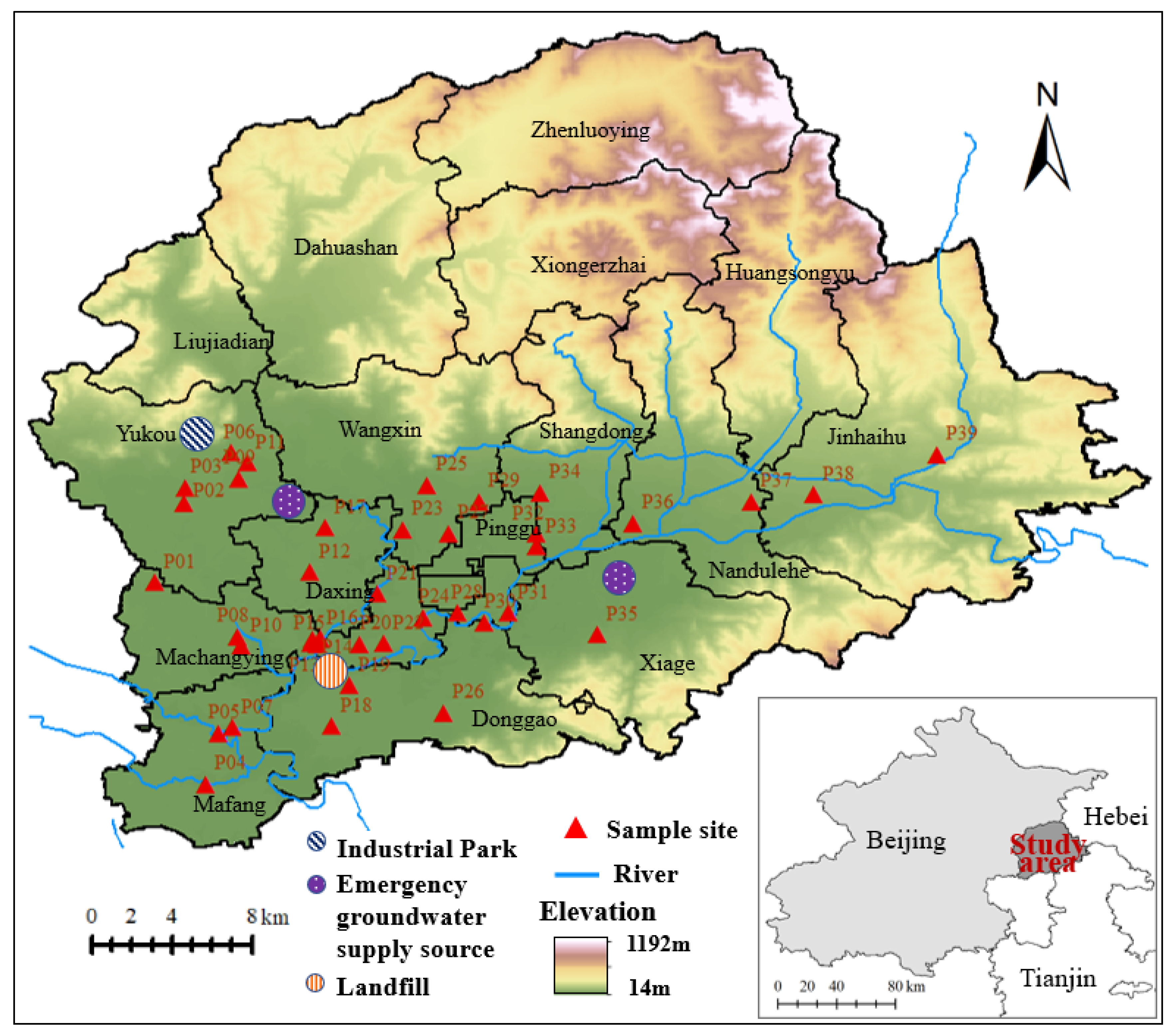
Pinggu district is northeast of Beijing, and borders Beijing, Tianjin, and Hebei; total area is 950.13 km². The study area is the plain of Pinggu (116°58′37″–117°18′42″ N, 40°2′19″–40°11′48″ E) (Figure 1), with an area of about 402 km², accounting for 42.3% of the total area. The study area has a temperate continental monsoon climate with distinct seasons: summers are rainy, and winters are dry. Annual average temperature is 11.7 °C. January is the coldest month, with an average temperature of 5.4 °C, and July is the hottest, with an average temperature of 26.1 °C; annual average precipitation is 636 mm. In 2014 and 2017, when two sampling campaigns were conducted, precipitation was 524 and 627 mm, respectively.

The lithology of the study area is mainly dolomite and sandstone. Bedrock is buried deep, with quaternary sediments overlaid on the top. The thickness of quaternary sediment varies greatly in different places due to the influence of topography and bedrock. There are 32 rivers in the study area, including three main rivers: Jv, Cuo, and Jinji. Jv is the longest river in Pinggu, with a total length of 54.15 km and a catchment area of 1692 km². The runoff flow direction of groundwater is basically consistent with the flow direction of the main rivers, and the underground runoff of the mountain area moves along the valley of the mountain area to the basin.

The study area is dominated by a loose layer of pore water that is widely distributed along the alluvial fan in the basin. The karst fissure water in Pinggu is mainly distributed in the mountainous areas around the basin and the underlying bedrock. In the plain area, the underlying bedrock at the top of the alluvial–diluvial fan is in direct contact with the quaternary gravelly pebbles, thus providing a good runoff channel for groundwater [19]. The yield of a single well in the strong water-rich area of the study area can reach 3000–5000 m³/d, and 1500–3000 m³/d in the medium water-rich area, while it is below 1500 m³/d in the weak water-rich area. Groundwater-recharge sources in the study area are mainly composed of atmospheric-precipitation infiltration recharge, surface-water infiltration recharge such as river channels, and lateral replenishment of the piedmont zone. Moreover, leakage from Haizi reservoir, flood infiltration, and the return infiltration of canals are also important supply sources. In addition, there are two emergency-water-supply sources in the study area that provide domestic water for Beijing.

3. Material and Methods

3.1. Sample Collection and Analysis

Two sampling campaigns were conducted in 39 groundwater-sampling sites (Figure 1) in August 2014 and 2017, and a total of 78 groundwater samples were collected. Before sampling, the in situ measurements of pH, temperature, TDS, and CO₂ were performed by portable meters. Sample bottles (clean polyethylene bottles) were rinsed by the same groundwater 2–3 times, and all samples were filtered with 0.45 m filter membranes and collected in the sample bottles. Nitric acid was also added to the sample used to test cations for pH < 2. After that, all samples were stored in ice boxes at 4 °C until laboratory analysis. An inductively coupled plasma spectrometer (ICP-9100) was used to analyze ion concentrations (K⁺, Na⁺, Ca²⁺, Mg²⁺, Mn). Ion chromatography (ICS-2500) was used to determine the concentrations of Cl⁻, SO₄²⁻, NO₃⁻, F⁻, and NH₄⁺. An iron–ion-concentration detector (JC503-ET7400, BW Electronic Technology Ltd., China) was used to determine the concentrations of Fe²⁺. Concentrations of HCO₃⁻ were determined by acid-base titration.

Laboratory quality-assurance and quality-control methods were used to ensure the quality of the analytical data, including standard calibration, the use of standard operating procedures, and reagent blank analysis. All analyses were performed in triplicate. Reagent blanks were monitored throughout analysis and used to correct analysis results.

3.2. Self-Organizing Maps (SOM)

SOM is an unsupervised artificial neural network model. Kohonen (1982) [20] proposed the SOM algorithm and introduced its specific implementation process. This method simulates the biological brain learning process that can make a cluster area form near each best-matching neuron, so that the input vectors of similar features are classified into a cluster. At the same time, SOM provides a visualization method of high-dimensional data projection in low-dimensional space, such as two-dimensional, while retaining the topological structure and metric relationships of the original data [21], which is suitable for high-dimensional data reduction, classification, and visualization. Heuristic rules can be used to select the appropriate number of neurons, such as $5\sqrt{\mathrm{n}}$ suggested by Vesanto et al. (2000) [22]. where n is the number of samples. The Davies–Bouldin index can be used to determine the optimal number of clusters [23]. The SOM algorithm can be run with MATLAB software, and it usually consists of the following steps: (i) setting variables and parameters, including input vector $\mathrm{X}\left(\mathrm{n}\right)$, weight vector W_i(n), and number of iterations $\mathrm{N}$; (ii) initializing weight vector W_i(n), setting initial learning rate ${\mathsf{\eta }}_0$, and normalizing the weight vector, initial value W_i(0), and input vector X(n); (iii) selecting training sample $\mathrm{X}{}^{\prime }$ from the input layer; (iv) calculating the Euclidean distance between ${\mathrm{W}}_{\mathrm{i}}{}^{\prime }$ and $\mathrm{X}{}^{\prime }$; (v) finding the best-matching unit (BMU) of the input sample according to Euclidean minimal principle

$$\Vert \mathrm{X}{}^{\prime }-{\mathrm{W}}_{\mathrm{c}}{}^{\prime }\Vert =\min \Vert \mathrm{X}{}^{\prime }-{\mathrm{W}}_{\mathrm{i}}{}^{\prime }\Vert =\min \left[{\mathrm{d}}_{\mathrm{i}}\right],\mathrm{i}=1,2\dots ,\mathrm{m},$$

(1)

and selecting winning neuron c through competitive learning; (ⅵ) updating the BMU and its neighbor neurons towards the input sample, and weight vector W_i at each time step t + 1 is calculated as follows:

$${\mathrm{W}}_{\mathrm{i}}(\mathrm{t}+1)={\mathrm{W}}_{\mathrm{i}}\left(\mathrm{t}\right)+{\mathsf{\eta }}_{\mathrm{t}}{\mathrm{h}}_{\mathrm{b}.\mathrm{i}}\left(\mathrm{t}\right)[\mathrm{X}-{\mathrm{W}}_{\mathrm{i}}(\mathrm{t}\left)\right];$$

(2)

(vii) iterating learning rate $\mathsf{\eta }$ and topology fields, and renormalizing the weights after learning; (viii) checking whether number of iterations $\mathrm{n}$ exceeds N, and if it does returning to Step (iii), otherwise, the iteration process ends.

4. Results

4.1. General Hydrochemical Characteristics

Table 1. Statistical summary of variables (unit: mg/L except for pH) in groundwater.

	Min	Max	Mean	C.V. (%)	Min	Max	Mean	C.V. (%)
	2014				2017
TDS	280	733	487	25.1	308	1090	561	32.3
pH	7.8	8.5	8.2	2.26	7.4	8.4	7.8	2.66
K+	0.45	3.5	1.66	46.7	0.23	2.97	1.40	47.8
Na+	5.87	50.5	16.5	72.1	5.41	47.9	18.8	69.4
Ca2+	37.7	124	68.7	28.2	32.9	191	78.3	42.5
Mg2+	18.8	51.9	30.3	24.9	19.6	66.1	31.5	29.9
NH4+	0.01	0.1	0.01	87.4	0.01	0.27	0.07	95.2
HCO3−	176	515	295	31.4	160	519	337	28.2
Cl−	0.4	48.4	14.2	99.4	3.01	85.4	22.1	105
SO42−	0.8	112	18.8	126	2.01	77.5	21.1	98.4
NO3−	0.4	165	26.8	149	0.2	275	35.2	144
F−	0.025	0.99	0.38	76.7	0.1	0.96	0.40	55.5
Fe2+	0.002	3.89	0.25	268	0.002	4.34	0.21	327
Mn	0.001	1.59	0.15	235	0.001	1.23	0.15	199
CO2	0	5.30	0.94	170	0	19.8	5.52	83.9

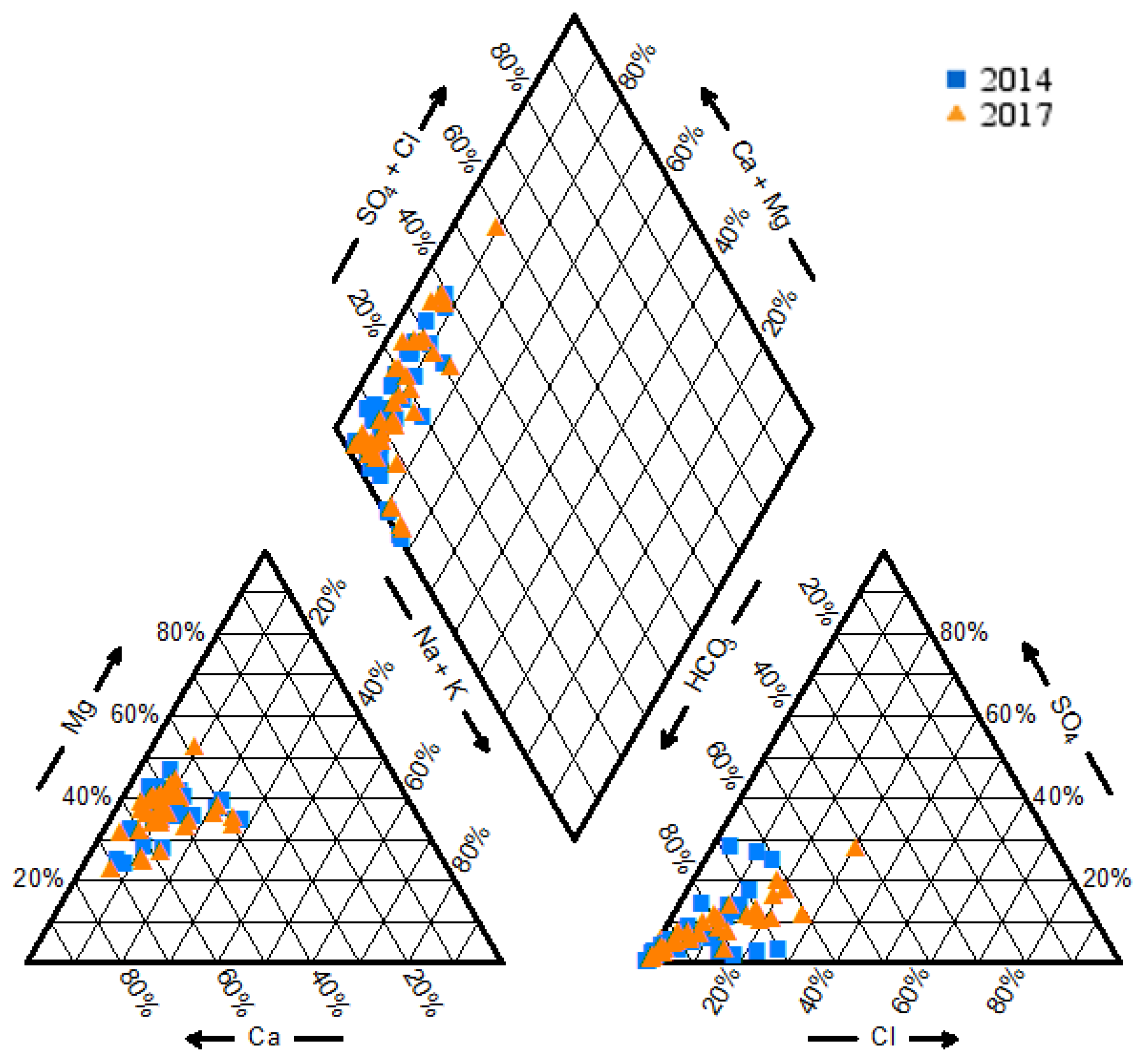
C.V.: coefficient of variation.

showed the statistical results of the hydrochemical parameters in the groundwater of the study area. Compared to 2014, the mean value of TDS was higher in 2017 (497 mg/L in 2014 and 561 mg/L in 2017), and 2014 groundwater was fresh water, but most 2017 sample sites were fresh water and a few were brackish water. The mean value of pH decreased in 2017 (8.2 in 2014 and 7.8 in 2017), but it remained weakly alkaline. In both 2014 and 2017, Ca²⁺ (37.7–124 mg/L in 2014, and 32.9–191 mg/L in 2017) was the dominant cation, while HCO₃⁻ (176–515 mg/L in 2014, and 160–519 mg/L in 2017) was the dominant anion. The piper diagram (Figure 2) showed that groundwater type in this area was HCO₃⁻Ca·Mg, and there was no significant change in 2014 and 2017. Among seven major ions, only the coefficient of variation (C.V.) of SO₄²⁻ (126% in 2014 and 98.4% in 2017) and Cl⁻ (99.4% in 2014 and 105% in 2017) were high, suggesting that concentrations had large variances in spatial distribution. NO₃⁻ is the commonly used indicator to study the impact of anthropogenic activities on groundwater. The maximal (165 mg/L in 2014 and 275 mg/L in 2017) and average values (26.8 mg/L in 2014 and 35.2 mg/L in 2017) of NO₃⁻ exceeded the 20 mg/L stipulated in Class III water in the Groundwater Quality Standard (GB/T 14848–2017), and both the maximal and the average value increased in 2017, which meant that the concentrations of NO₃⁻ may have been impacted by anthropogenic activities, and the high C.V. (149% in 2014 and 144% in 2017) of NO₃⁻ also supported this view. In addition, the C.V. of Fe²⁺, Mn, and NH₄⁺ were high, and NO₃⁻, NH₄⁺, Fe²⁺, and Mn were sensitive to the redox state of groundwater. The high C.V. of these parameters indicated that the redox status of groundwater in the study area also varied.

4.2. Correlation and Saturation Index Analysis

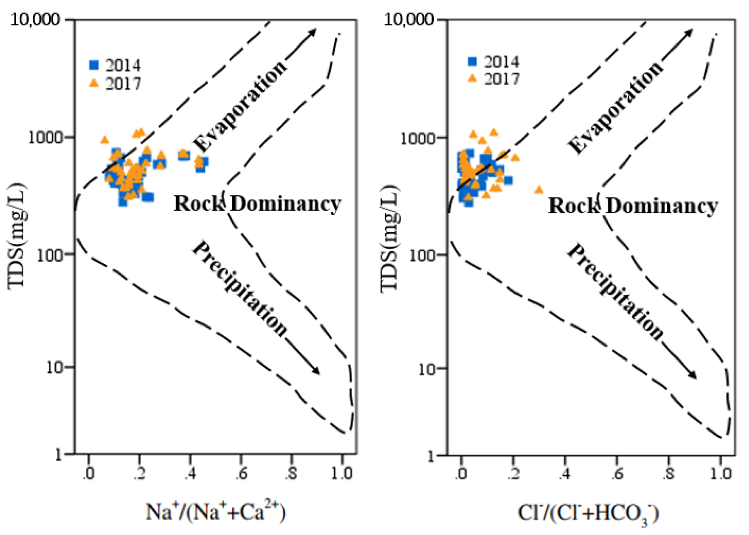
According to the Gibbs diagram (Figure 3), water chemistry in the study area was controlled by rock weathering. The Spearman correlation coefficient (

Table 2. Correlation coefficients for groundwater variables.

	K+	Na+	Ca2+	Mg2+	NH4+	HCO3−	Cl−	SO42−	NO3−	F−	Fe2+	Mn	TDS	CO2	pH
K+	1.00	0.25 *	0.02	0.28 *	0.09	0.25 *	−0.16	−0.10	−0.18	0.24 *	0.15	0.23 *	0.19	−0.04	0.20
Na+		1.00	0.48 **	0.52 **	0.20	0.73 **	−0.04	−0.12	−0.31 **	0.12	0.42 **	0.53 **	0.71 **	0.27 *	−0.09
Ca2+			1.00	0.68 **	0.08	0.60 **	0.51 **	0.40 **	0.24 *	−0.25 *	0.12	0.18	0.87 **	0.44 **	−0.19
Mg2+				1.00	0.07	0.57 **	0.18	0.12	0.08	−0.07	0.17	0.25 *	0.83 **	0.25 *	−0.03
NH4+					1.00	0.25 *	0.07	−0.06	−0.06	0.16	0.44 **	0.58 **	0.21	0.43 **	−0.39 **
HCO3−						1.00	0.00	−0.08	−0.30 **	0.22 *	0.33 **	0.54 **	0.82 **	0.45 **	−0.27 *
Cl−							1.00	0.81 **	0.64 **	−0.33 **	−0.04	0.06	0.26 *	0.37 **	−0.11
SO42−								1.00	0.66 **	−0.20	−0.22 *	−0.04	0.15	0.31 **	−0.09
NO3−									1.00	−0.39 **	−0.11	−0.19	0.00	0.17	0.03
F−										1.00	0.11	0.21	−0.09	0.04	0.05
Fe2+											1.00	0.55 **	0.28 *	0.17	−0.13
Mn												1.00	0.45 **	0.51 **	−0.47 **
TDS													1.00	0.50 **	−0.28 *
CO2														1.00	−0.78 **
pH															1.00

** Correlation is significant at the 0.01 level (2-tailed). * Correlation is significant at the 0.05 level (2-tailed).

) showed that the positive correlation coefficients between Ca²⁺, Mg²⁺, and HCO₃⁻ were higher, and TDS showed a high positive correlation with Na⁺ (0.71), Ca²⁺ (0.87), Mg²⁺ (0.83), and HCO₃⁻ (0.82), and the correlation between Na⁺ and HCO₃⁻ was also high (0.73), which indicated that Na⁺, Ca²⁺, Mg²⁺, and HCO₃⁻ may have common sources. There was no obvious correlation between Na⁺ and Cl⁻, and Ca²⁺ and SO₄²⁻, indicating that evaporite dissolution may not be the dominant process. There was a clear positive correlation between Cl⁻, SO₄²⁻, and NO₃⁻, and combined with their high C.V. in Table 1, it can be inferred that Cl⁻, SO₄²⁻, and NO₃⁻ may have originated from the same anthropogenic activities.

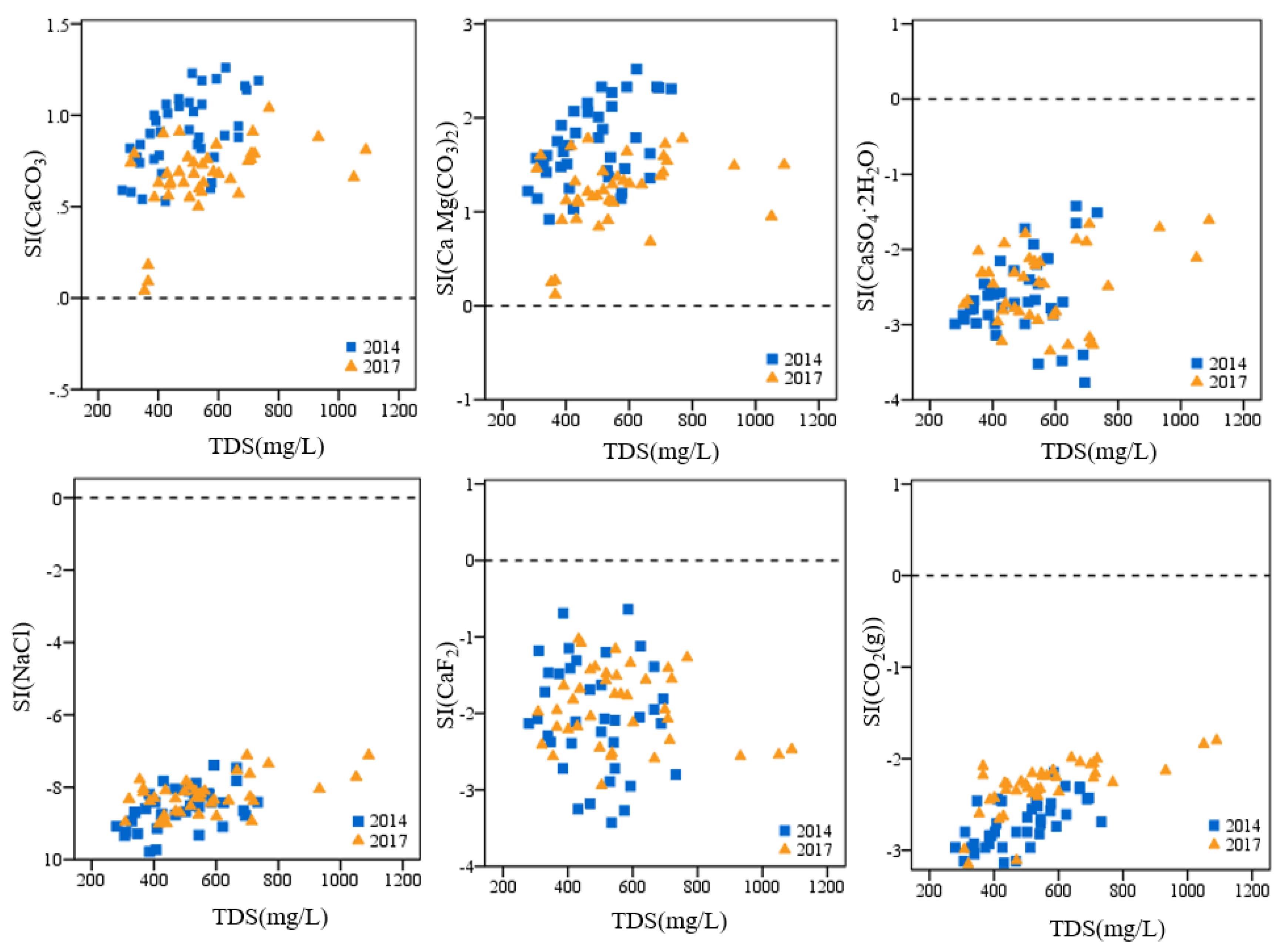
In order to further study the effect of water–rock interactions on groundwater chemical evolution, PHREEQC software was used to calculate the saturation index (SI) of calcite (CaCO₃), dolomite (CaMg(CO₃)₂), gypsum (CaSO₄·H₂O), halite (NaCl), fluorite (CaF₂), and CO₂ (g) (Figure 4). Both calcite and dolomite were oversaturated, but gypsum, halite, and fluorite were undersaturated. The SI of CO₂ (g) were −3.18 to 1.8, showing an upward trend with the increase in TDS. Compared to 2014, the SI of CO₂ (g) was higher in 2017, but the SI of calcite and dolomite was lower. It seems that some external factor caused this opposite result, which we further discuss below.

4.3. SOM Results

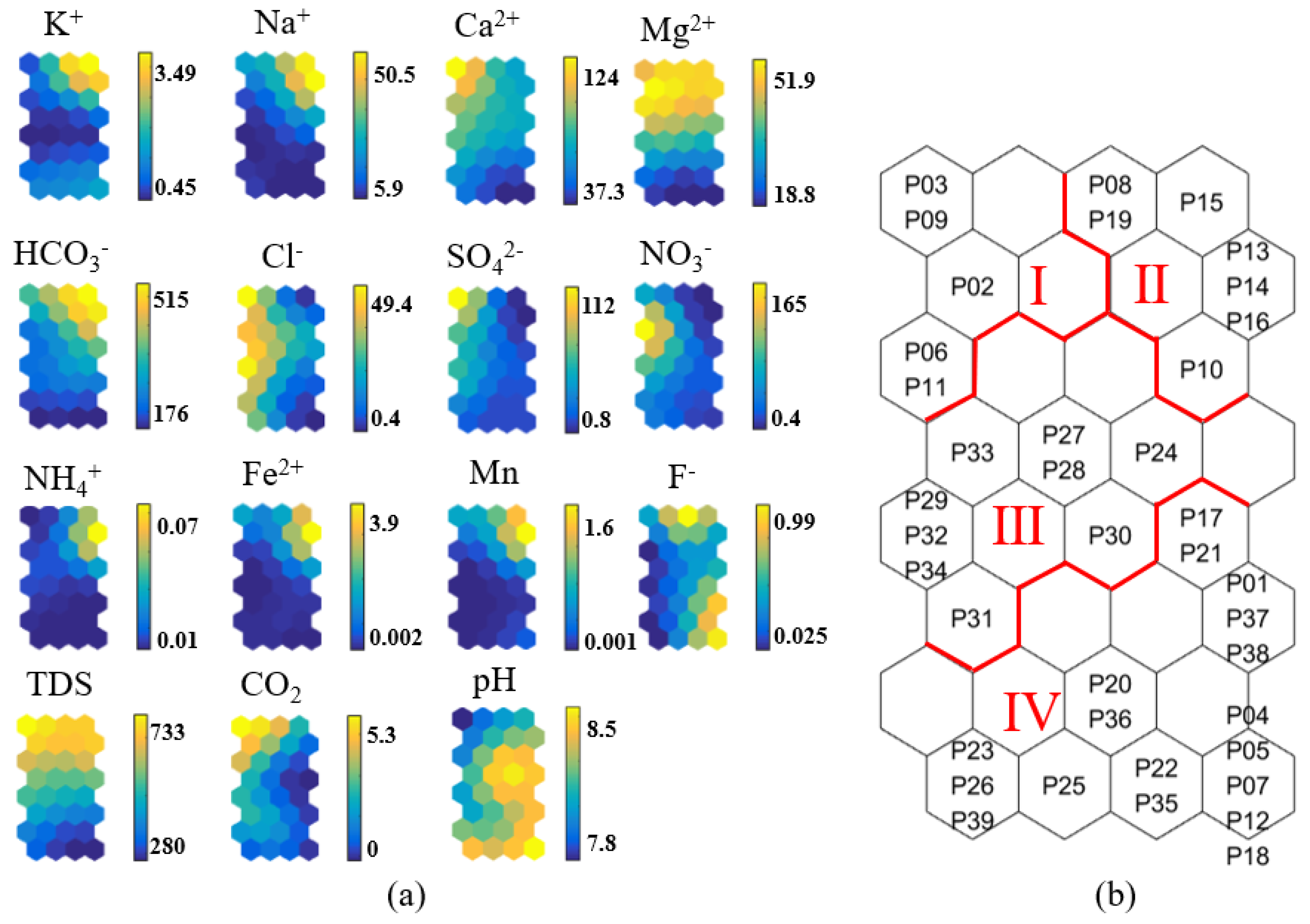
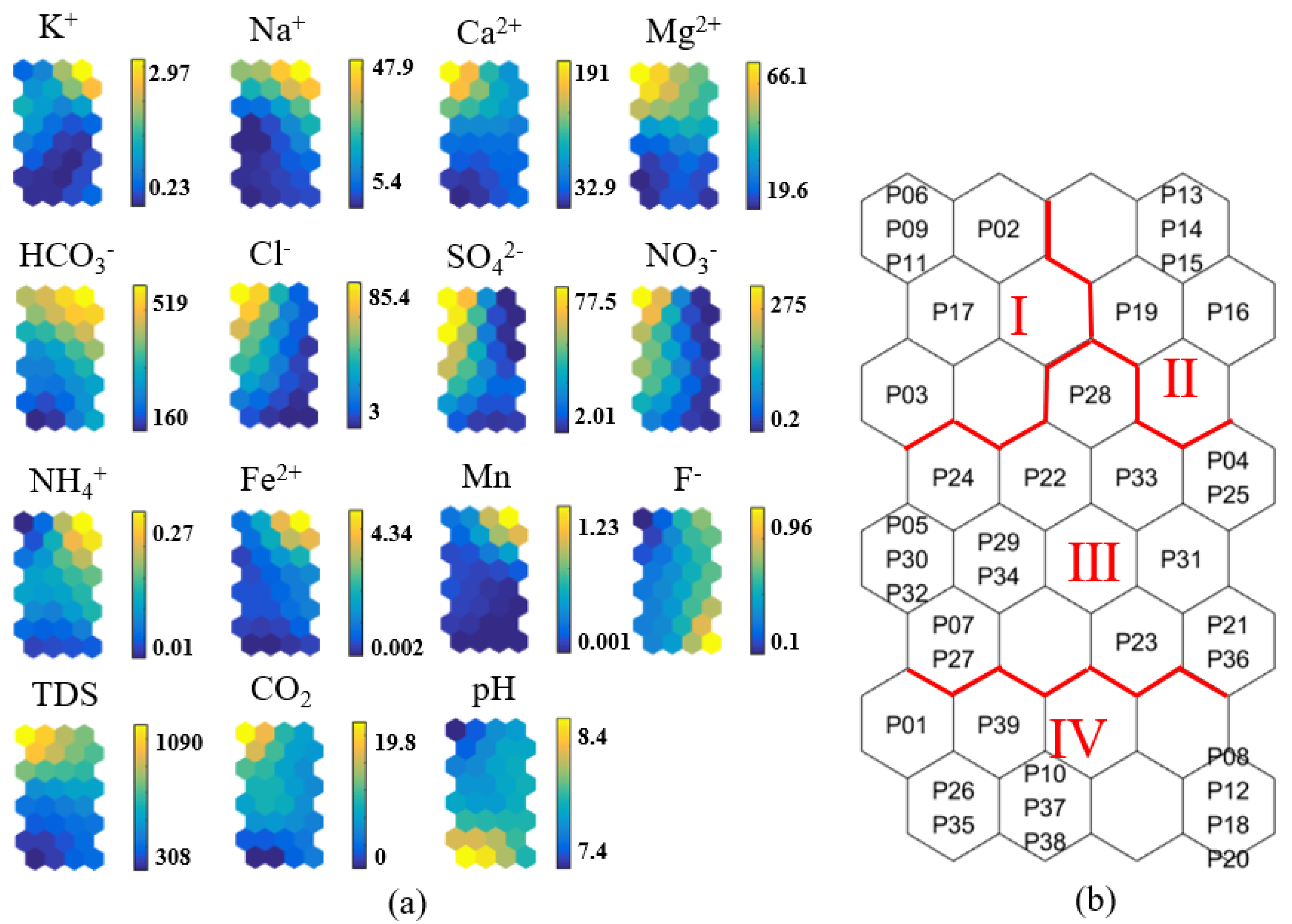
The SOM was used to analyze groundwater data in 2014 and 2017 (n = 39). Thirty-two (8 × 4) output neurons were selected (Figure 5a and Figure 6a), and sampling points were grouped into four clusters (Figure 5b and Figure 6b). Neurons use color codes to display the weight-vector value of each neuron. Blue and yellow correspond to low and high concentrations of parameters, respectively. Therefore, the interdependence of variables can be identified through the color comparison of neurons. Figure 5a showed that HCO₃⁻, Na⁺, and K⁺ had similar color gradients, indicating that they may be controlled by the same hydrochemical processes. Cl⁻, SO₄²⁻, and NO₃⁻ showed a negative correlation with HCO₃⁻, Na⁺, and K⁺ by the inverse color gradient, which suggested that Cl⁻, SO₄²⁻, and NO₃⁻ were controlled by different sources from HCO₃⁻, Na⁺, and K⁺. Fe²⁺, Mn, and NH₄⁺ had obvious similarities in color gradient, indicating that they relied on common water chemical processes, such as redox reactions. Compared with the 2014 results, the 2017 results (Figure 6a) showed greater similarities in the color gradients of Cl⁻, SO₄²⁻, and NO₃⁻; in combination with the high C.V. of these parameters, shown in Table 1, it could be inferred that anthropogenic factors controlling their concentrations were strengthened in 2017, such as sewage discharge and pesticide use.

Figure 5b showed that five (12.8%) sample sites were classified in Cluster I, 7 (17.9%) sample sites were classified in Cluster II, nine (23%) sample sites were classified in Cluster III, and 18 (46.3%) sample sites were classified in Cluster IV. In 2017 (Figure 6b), six sample sites were classified in Cluster I, five sample sites were classified in Cluster II, 17(43.6%) sample sites were classified in Cluster III, and 11 (28.2%) sample sites were classified in Cluster IV. Obviously, the number of Clusters III and IV changed dramatically in 2017 compared to 2014, which might have been due to the increased anthropogenic activities in Cluster III or IV.

Table 3. Statistical summary of variables in four clusters in 2014 and 2017.

		N	TDS	pH	K+	Na+	Ca2+	Mg2+	NH4+	HCO3−	Cl−	SO42−	NO3−	F−	Fe2+	Mn	CO2
C1	2014	5	643.2	7.95	1.22	16.8	101.3	38.1	0.01	303.6	26.6	58.9	78.5	0.20	0.32	0.18	3.08
	2017	6	857.7	7.61	1.40	26.6	139.0	44.1	0.01	396.7	59.9	59.5	93.2	0.18	0.09	0.12	12.0
C2	2014	7	621.6	8.13	2.93	37.7	70.7	37.3	0.03	450.1	9.2	3.9	2.8	0.46	0.94	0.63	1.26
	2017	5	680.0	7.78	2.48	40.3	80.9	34.9	0.18	470.6	14.0	3.5	1.1	0.53	1.17	0.77	5.28
C3	2014	9	503.1	8.18	1.08	10.9	76.6	31.9	0.01	275.6	22.3	27.5	43.4	0.20	0.04	0.00	0.78
	2017	17	512.7	7.79	1.25	14.4	70.2	29.7	0.08	324.0	29.8	31.8	47.8	0.37	0.09	0.05	5.49
C4	2014	18	382.4	8.23	1.59	10.9	55.0	24.6	0.01	243.0	8.6	9.1	13.6	0.49	0.07	0.04	0.29
	2017	11	418.5	8.02	1.15	11.5	56.4	26.0	0.02	265.5	8.8	9.4	15.0	0.49	0.03	0.02	2.12

C = Cluster. N = Number of samples.

showed the average value of the parameters in each cluster. Concentrations of Ca²⁺, Mg²⁺, Cl⁻, SO₄²⁻, and NO₃⁻ in the first cluster were the highest in both 2014 and 2017 between the four clusters, and concentrations increased further in 2017. The concentrations of NH₄⁺, Fe²⁺, and Mn in Cluster II were the highest in both 2014 and 2017, while concentrations of SO₄²⁻ and NO₃⁻ were very low and further reduced in 2017. Concentrations of Cl⁻, SO₄²⁻, and NO₃⁻ in Cluster III were second only to those in Cluster I, and all their concentrations increased in 2017. The concentrations of all parameters were small in Cluster IV, and did not change significantly in either 2014 or 2017. It follows that the increase in sample sites in Cluster III might have been because of active anthropogenic factors in the area of Cluster III.

To study differences between clusters, a Mann–Whitney nonparametric test was performed (

Table 4. Results of Mann–Whitney test in water chemistry between 2014 and 2017 clusters.

Year	Ⅰvs.Ⅱ		Ⅰvs.Ⅲ		Ⅰvs.Ⅳ		Ⅱvs.Ⅲ		Ⅱvs.Ⅳ		Ⅲvs.Ⅳ
	2014	2017	2014	2017	2014	2017	2014	2017	2014	2017	2014	2017
TDS	0.81	0.27	*	*	*	*	*	*	*	*	*	*
pH	0.12	*	*	*	*	*	0.67	0.58	0.23	*	0.68	*
K+	*	0.1	0.55	1	0.16	0.92	*	*	*	*	*	0.19
Na+	*	0.14	*	0.14	0.09	*	*	*	*	*	0.88	0.34
Ca2+	*	*	*	*	*	*	0.31	0.33	*	*	*	*
Mg2+	0.81	0.14	0.23	*	*	*	0.1	0.13	*	*	*	0.17
NH4+	*	*	0.27	*	1	0.35	*	*	*	*	1	*
HCO3−	*	0.12	0.46	*	0.1	*	*	*	*	*	0.11	*
Cl−	*	*	0.46	*	*	*	*	*	0.25	*	*	*
SO42−	*	*	0.46	*	*	*	*	*	*	*	*	*
NO3−	*	*	0.46	*	*	*	*	*	*	*	*	*
F−	0.09	*	0.64	*	0.06	*	*	0.6	0.9	0.43	*	0.38
CO2	0.15	*	*	*	*	*	0.67	0.64	0.08	*	0.18	*
Fe2+	*	*	0.52	0.48	0.939	0.24	*	*	*	*	0.37	*
Mn	*	*	0.12	0.87	0.07	0.17	*	*	*	*	0.48	0.1

* p < 0.05.

). In 2014 (Table 4a), anthropogenic parameters such as Cl⁻, NO₃⁻, and SO₄²⁻ had significant differences with several clusters (Clusters I and II, Clusters I and IV, Clusters II and III, and Clusters III and IV). In 2017 (Table 4b), these three parameters had significant differences in all clusters, which indicated that anthropogenic activities affecting groundwater composition increased in these three years. Concentrations of NO₃⁻, SO₄²⁻, NH₄⁺, Fe²⁺ and Mn were significantly different between Cluster II and the other clusters, indicating that parameters that are sensitive to the redox state of groundwater play an important role in the classification of Cluster II and the other clusters.

5. Discussion

5.1. Formation Mechanisms of Groundwater Chemistry

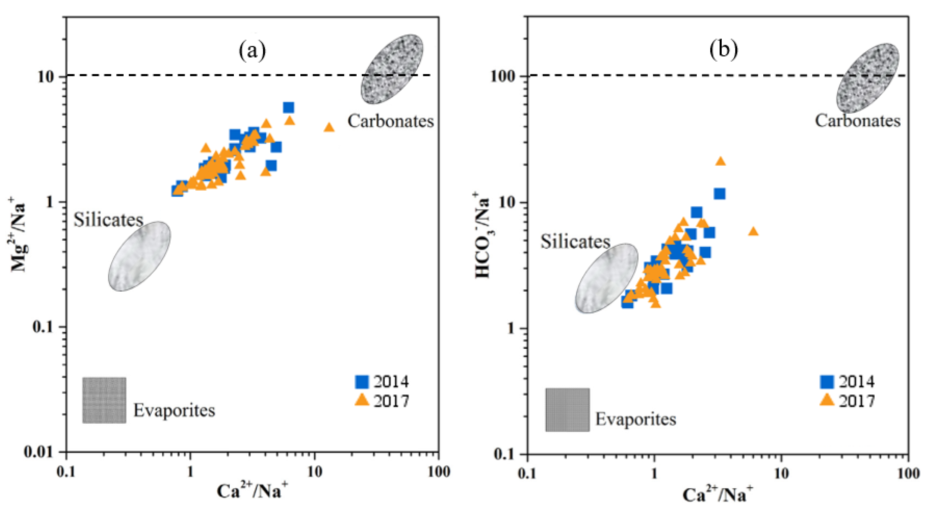
The groundwater type of the study area is HCO₃-Ca·Mg (Figure 2), and the main processes that control it are water–rock interactions (Figure 3). According to correlation analysis and the SI of minerals, it could be inferred that the groundwater in this area may have undergone carbonate and silicate weathering (Equations (3)–(5)), and the results of Figure 7 also supported this inference. The negative correlation between SI (CO₂) and TDS might be due to the groundwater being dominated by dissolved carbonate having low salinity and CO₂ as the reactant of carbonate dissolution, the SI of which would show a downward trend with the decrease in TDS. Compared to 2014, the SI of CO₂ (g) was higher in 2017. This is probably because the higher precipitation in 2017 (627 mm in 2017 and 524 mm in 2014) brought more CO₂ and diluted the groundwater at the same time, which lowered the SI of calcite and dolomite in 2017.

In this study, the concentration of F⁻ did not exceed the 1 mg/L stipulated for Class III water in the Groundwater Quality Standard (GB/T 14848–2017), and no obvious aggregation occurred in space distribution. Therefore, in combination with the small C.V. in Table 1, it was speculated that the concentration of F⁻ was not mainly affected by anthropogenic activities. Choi et al. (2013) [24] found high F⁻ concentrations in alkaline HCO₃-Na type groundwater. Although the groundwater chemical type in this study area was HCO₃-Ca·Mg, silicate weathering still existed that could release Na⁺ in the groundwater. Thus, the coexistence of HCO₃⁻ and Na⁺ in groundwater was still beneficial for the enrichment of F⁻. The pH was alkaline (7.4–8.5), which is also conducive to enriching F⁻. Choi et al. (2013) [24] also found that Ca²⁺ plays an important role in controlling F⁻ concentration in groundwater. In this study, groundwater was supersaturated for both calcite and dolomite, but unsaturated for fluorite. This indicated that a high concentration of Ca²⁺ is enough to maintain supersaturation with calcite and dolomite. However, groundwater cannot reach saturation with fluorite because fluorite saturation is dependent on the availability of F⁻ in groundwater.

$$\begin{array}{l}\mathrm{Na},\mathrm{K},\mathrm{Mg},\mathrm{Casilicate}+{\mathrm{CO}}_2+{\mathrm{H}}_2\mathrm{O}\\ \to {\mathrm{H}}_4{\mathrm{SiO}}_4+{\mathrm{HCO}}_3^{-}+{\mathrm{Na}}^{+}+{\mathrm{K}}^{+}+{\mathrm{Ca}}^{2+}+{\mathrm{Mg}}^{2+}+\mathrm{Solids}\end{array}$$

(3)

$${\mathrm{CaCO}}_3+{\mathrm{CO}}_2+{\mathrm{H}}_2\mathrm{O}\stackrel{ }{\iff }{\mathrm{Ca}}^{2+}+2{\mathrm{HCO}}_3{}^{-}$$

(4)

$$\mathrm{CaMg}{\left({\mathrm{CO}}_3\right)}_2+{\mathrm{CO}}_2+2{\mathrm{H}}_2\mathrm{O}\stackrel{ }{\iff }{\mathrm{Ca}}^{2+}+{\mathrm{Mg}}^{2+}+4{\mathrm{HCO}}_3{}^{-}$$

(5)

5.2. Spatiotemporal Variations

Groundwater is not only controlled by the natural processes analyzed above, but also affected by anthropogenic activities, which could be derived from the SOM results.

According to the spatial distribution of the sample sites (Figure 1), the Cluster I sample sites were located northwest of the study area. Concentrations of Cl⁻, SO₄²⁻, NO₃⁻, Ca²⁺, and Mg²⁺ were the highest of the four clusters, and concentrations in 2017 were even higher. Cl⁻, SO₄²⁻, and NO₃⁻ in groundwater typically come from domestic wastewater, agricultural chemicals, industrial chemicals, and surface water [25]. According to the field investigation, Yukou Industrial Park and large areas of farmland are located here; therefore, there are two sources of pollution around Cluster I, industrial and agricultural sources. Yukou Industrial Park focuses on the development of three major industrial chains, electromechanical electronics, clothing, and food brewing. Sewage from clothing-manufacturing and food-brewing processes could increase Cl⁻, SO₄²⁻, and NO₃⁻ concentrations in groundwater. Discharged wastewater from the electronic-device factory would increase the concentrations of Ca²⁺, Mg²⁺, and other metal ions. Pinggu district is an important agricultural product base of Beijing, and NH₄Cl and (NH₄)₂SO₄ contained in agricultural fertilizers could enter groundwater through precipitation leaching. A large area of orchards is also located here, and orchards must be sprayed with pesticides (such as Bordeaux mixture). CuSO₄, as an important component of Bordeaux mixture, can increases concentrations of SO₄²⁻ in groundwater. Moreover, in 2017 (Figure 6a), color-gradient similarities of Cl⁻, SO₄²⁻, and NO₃⁻ strengthened, which demonstrated that the impact of industrial and agricultural activities on groundwater increased in 2017. Furthermore, industrial sewage is mainly acidic, which reduced the pH and increased CO₂ concentrations of Cluster I groundwater in 2017 compared to 2014.

Cluster II was concentrated near the Qianruiying landfill southwest of the study area. Qianruiying was built in 2000 with an area of 11,000 m². Reductive refuse leachate enters groundwater directly without oxidation in a relatively hermetical environment where the refuse is piled up. Therefore, concentrations of NH₄⁺, Fe²⁺, and Mn were very high, and Mn could easily be soluble in water under hypoxic conditions, existing in the form of Mn²⁺. Accordingly, concentrations of NO₃⁻ and SO₄²⁻ were low because they were reduced, and concentrations of NO₃⁻ and SO₄²⁻ were further reduced in 2017 compared to 2014.

As for Cluster III, sample sites were concentrated in the town of Pinggu, which is densely populated and the most prosperous place of the study area. Hence, the discharge of domestic sewage is the main source of groundwater pollution. Concentrations of Cl⁻, SO₄²⁻, and NO₃⁻ were the second highest after Cluster I. The sample sites increased substantially in 2017, and those increased sample sites were mainly distributed in two areas, around the towns of (i) Pinggu and (ii) Mafang, in the southwest of the study area (P04, P05, P07). There are dense villages around Pinggu, drainage facilities in these villages are rudimentary, and villagers often spill domestic sewage directly on the bare ground. It is easy for sewage to contaminate groundwater on account of less asphalt pavement in the villages. Sample sites near Mafang were classified as Cluster III in 2017 for two reasons. First, the study area is surrounded by mountains on three sides. Mafang is the only “exit” of the plain area, so traffic there is heavy, and its population is growing rapidly. However, drainage and sewage-treatment facilities have not improved, which tends to make the groundwater quality of Mafang deteriorate; second, the elevation of Mafang is the lowest, making this a sink of groundwater runoff, and the groundwater containing Cl⁻, SO₄²⁻, and NO₃⁻ converges here, which affects Mafang’s groundwater quality to some extent.

The sample sites of Cluster IV were distributed at the edge of the study area and sparsely populated areas. The concentrations of pollution indicators in this cluster were relatively low, and few changes occurred in 2014 and 2017. It can be inferred that Cluster IV represents groundwater that is less affected by anthropogenic activities. Nevertheless, the area covered by this cluster in 2017 was diminished compared to 2014, which indicated that groundwater quality in the study area deteriorated in 2017.

6. Conclusions

The type of groundwater in the Pinggu plain area is HCO₃-Ca·Mg, with a TDS of 280–1090 mg/L. Groundwater quality is affected by both natural and anthropogenic factors. Natural factors are mainly dominated by carbonate and silicate weathering, and anthropogenic factors mainly come from industrial activities, agricultural activities, landfills, and domestic-sewage discharge.

Large-scale farming and intense industrial activities in the northwest of the study area have increased the concentrations of Cl⁻, SO₄²⁻, NO₃⁻, Ca²⁺ and Mg²⁺ in groundwater by using pesticides and discharging industrial sewage. In the southwest of the study area, NH₄⁺, Fe²⁺, and Mn concentrations are mainly caused by refuse landfill activities. Areas affected by domestic-sewage discharge were around densely populated towns (Pinggu and Mafang), where Cl⁻, SO₄²⁻, and NO₃⁻ concentrations were high. Compared to 2014, areas with good groundwater quality that was not affected by human activities decreased in 2017. Thus, measures must be taken to prevent the further deterioration of groundwater quality.

Existing problems and related suggestions are as follows: (i) the discharge of industrial and domestic sewage should be strictly monitored in accordance with the relevant quality standards, pesticide-usage modes and dosages should be standardized, and effective treatment measures should be taken in heavily polluted agricultural areas and landfills; (ii) the area of groundwater affected by domestic-sewage discharge has increased, so it is necessary to improve drainage and sewage-treatment facilities in villages, and strengthen the education of villagers; (iii) the groundwater quality of Mafang in the southwest deteriorated due to rapid urban development, so the speed of upgrading drainage and sewage-treatment facilities should keep up with the speed of urban development, and relevant laws and regulations should be improved for areas with rapid development, which can prevent groundwater pollution from hindering urban development. The above suggestions provide ideas for the management of groundwater quality in other rapidly developing urban areas.

References

- Huang, G.; Sun, J.; Zhang, Y.; Chen, Z.; Liu, F. Impact of anthropogenic and natural processes on the evolution of groundwater chemistry in a rapidly urbanized coastal area, South China. Sci. Total Environ. 2013, 463–464, 209–221. [Google Scholar] [CrossRef] [PubMed]
- Xiao, J.; Jin, Z.; Wang, J. Assessment of the hydrogeochemistry and groundwater quality of the Tarim River Basin in an extreme arid region, NW China. Environ. Manag. 2014, 53, 135–146. [Google Scholar] [CrossRef] [PubMed]
- Li, P.; Wu, J.; Qian, H.; Lyu, X.; Liu, H. Origin and assessment of groundwater pollution and associated health risk: A case study in an industrial park, northwest China. Environ. Geochem. Health 2014, 36, 693–712. [Google Scholar] [CrossRef] [PubMed]
- Monjerezi, M.; Vort, R.D.; Aagaard, P.; Saka, J.D.K. Hydro-geochemical processes in an area with saline groundwater in lower Shire River valley, Malawi: An integrated application of hierarchical cluster and principal component analyses. Appl. Geochem. 2011, 26, 1399–1413. [Google Scholar] [CrossRef]
- Yan, B.; Xiao, C.; Liang, X.; Fang, Z. Impacts of urban land use on nitrate contamination in groundwater, Jilin City, Northeast China. Arab. J. Geosci. 2016, 9, 105. [Google Scholar] [CrossRef]
- Lu, H.; Yin, C. Shallow groundwater nitrogen responses to different land use managements in the riparian zone of Yuqiao Reservoir in North China. J. Environ. Sci. 2008, 20, 652–657. [Google Scholar] [CrossRef] [Green Version]
- Gurunadha Rao, V.V.S.; Tamma Rao, G.; Surinaidu, L.; Mahesh, J.; Mallikharjuna Rao, S.T.; Mangaraja Rao, B. Assessment of geochemical processes occurring in groundwaters in the coastal alluvial aquifer. Environ. Monit. Assess. 2013, 185, 8259–8272. [Google Scholar] [CrossRef]
- Sahraei Parizi, H.; Samani, N. Geochemical evolution and quality assessment of water resources in the Sarcheshmeh copper mine area (Iran) using multivariate statistical techniques. Environ. Earth Sci. 2013, 69, 1699–1718. [Google Scholar] [CrossRef]
- Pant, R.R.; Zhang, F.; Rehman, F.U.; Wang, G.; Ye, M.; Zeng, C.; Tang, H. Spatiotemporal variations of hydrogeochemistry and its controlling factors in the Gandaki River Basin, Central Himalaya Nepal. Sci. Total Environ. 2018, 622–623, 770–782. [Google Scholar] [CrossRef]
- Güler, G.; Kurt, M.A.; Alpaslan, M.; Akbulut, C. Assessment of the impact of anthropogenic activities on the groundwater hydrology and chemistry in Tarsus coastal plain (Mersin, SE Turkey) using fuzzy clustering, multivariate statistics and GIS techniques. J. Hydrol. 2012, 414–415, 435–451. [Google Scholar] [CrossRef]
- Reghunath, R.; Sreedhara Murthy, T.R.; Raghavan, B.R. The utility of multivariate statistical techniques in hydrogeochemical studies: An example from Karnataka, India. Water Res. 2002, 36, 2437–2442. [Google Scholar] [CrossRef]
- Lischeid, G. Non-linear visualization and analysis of large water quality data sets: A model-free basis for efficient monitoring and risk assessment. Stoch. Environ. Res. Risk Assess. 2009, 23, 977–990. [Google Scholar] [CrossRef]
- Wongravee, K.; Lloyd, G.R.; Silwood, C.J.; Crootveld, M.; Brereton, R.G. Supervised Self Organization Maps for classification and determination of potentially discriminatory variables: Illustrated by application to nuclear magnetic resonance metabolomic profiling. Anal. Chem. 2010, 82, 628–638. [Google Scholar] [CrossRef] [PubMed]
- Güler, C.; Thyne, G.D.; McCray, J.E.; Turner, A.K. Evaluation of graphical and multivariate statistical methods for classification of water chemistry data. Hydrogeol. J. 2002, 10, 455–474. [Google Scholar] [CrossRef]
- Nguyen, T.T.; Kawamura, A.; Tong, T.N.; Nakagawa, N.; Amaguchi, H.; Gilbuena, R., Jr. Clustering spatio–seasonal hydrogeochemical data using Self-Organizing Maps for groundwater quality assessment in the Red River Delta, Vietnam. J. Hydrol. 2015, 522, 661–673. [Google Scholar] [CrossRef]
- Pearce, A.R.; Rizzo, D.M.; Mouser, P.J. Subsurface characterization of groundwater contaminated by landfill leachate using microbial community profile data and a nonparametric decision-making process. Water Resour. Res. 2011, 47, W06511. [Google Scholar] [CrossRef] [Green Version]
- Skwarzec, B.; Kabat, K.; Astel, A. Seasonal and spatial variability of 210Po, 238U and 239+240Pu levels in the river catchment area assessed by application of neural network based classification. J. Environ. Radioact. 2009, 100, 167–175. [Google Scholar] [CrossRef]
- Zelazny, M.; Astel, A.; Wolanin, A.; Malek, S. Spatiotemporal dynamics of spring and stream water chemistry in a high-mountain area. Environ. Pollut. 2011, 159, 1048–1057. [Google Scholar] [CrossRef]
- Yang, Q.C.; Liang, J.; Liu, L.C. Numerical Model for the Capacity Evaluation of Shallow Groundwater Heat Pumps in Beijing Plain, China. Procedia Environ. Sci. 2011, 10, 881–889. [Google Scholar] [CrossRef] [Green Version]
- Kohonen, T. Self-organized formation of topologically correct feature maps. Biol. Cybern. 1982, 43, 59–69. [Google Scholar] [CrossRef]
- Hazrati, Y.S.; Datta, B. Adaptive surrogate model based Optimization (ASMBO) for unknown groundwater contaminant source characterizations using Self-Organizing Maps. J. Water Resour. Prot. 2017, 9, 193–214. [Google Scholar] [CrossRef] [Green Version]
- Vesanto, J.; Himberg, J.; Alhoniemi, E.; Parhankangas, J. SOM Toolbox for Matlab 5, Report A57; Helsinki University of Technology: Espoo, Finland, 2000. [Google Scholar]
- Wang, C.; Lek, S.; Lai, Z.; Tudesque, L. Morphology of Aulacoseira filaments as indicator of the aquatic environment in a large subtropical river: The Pearl River, China. Ecol. Indic. 2017, 81, 325–332. [Google Scholar] [CrossRef]
- Choi, B.Y.; Yun, S.T.; Kim, K.H.; Kim, J.W.; Kim, H.M.; Koh, Y.K. Hydrogeochemical interpretation of South Korean groundwater monitoring data using Self-Organizing Maps. J. Geochem. Explor. 2013, 137, 73–84. [Google Scholar] [CrossRef]
- McArthur, J.M.; Sikdar, P.K.; Hoque, M.A.; Ghosal, U. Waste-water impacts on groundwater: Cl/Br ratios and implications for arsenic pollution of groundwater in the Bengal Basin and Red River Basin, Vietnam. Sci. Total Environ. 2012, 437, 390–402. [Google Scholar] [CrossRef] [PubMed] [Green Version]
Figure 1.
Location map of study area and spatial distribution of sample sites.
Figure 2.
Piper diagram of major ions in groundwater of 2014 and 2017.
Figure 3.
Spatiotemporal variation in weight ratio of Na+/(Na+ + Ca2+) and Cl−/(Cl− + HCO3−) as TDS function in Gibbs diagram of 2014 and 2017.
Figure 4.
Scatter plot of groundwater mineral saturation index of 2014 and 2017.
Figure 5.
SOM results of 2014: (a) the SOM visualization of groundwater chemicals, the numbers indicate values of the corresponding variables; (b) the clustering pattern in the SOM, the number in a hexagon denotes the sample number of groundwater.
Figure 6.
SOM results of 2017: (a) the SOM visualization of groundwater chemicals, the numbers indicate values of the corresponding variables; (b) the clustering pattern in the SOM, the number in a hexagon denotes the sample number of groundwater.
Figure 7.
Mixing diagram of Na normalized molar ratios of (a) Ca2+ versus Mg2+ and (b) Ca2+ versus HCO3− in 2014 and 2017.