Role of Cluster Validity Indices in Delineation of Precipitation Regions

Abstract

The delineation of precipitation regions is to identify homogeneous zones in which the characteristics of the process are statistically similar. The regionalization process has three main components: (i) delineation of regions using clustering algorithms, (ii) determining the optimal number of regions using cluster validity indices (CVIs), and (iii) validation of regions for homogeneity using L-moments ratio test. The identification of the optimal number of clusters will significantly affect the homogeneity of the regions. The objective of this study is to investigate the performance of the various CVIs in identifying the optimal number of clusters, which maximizes the homogeneity of the precipitation regions. The k-means clustering algorithm is adopted to delineate the regions using location-based attributes for two large areas from Canada, namely, the Prairies and the Great Lakes-St Lawrence lowlands (GL-SL) region. The seasonal precipitation data for 55 years (1951–2005) is derived using high-resolution ANUSPLIN gridded point data for Canada. The results indicate that the optimal number of clusters and the regional homogeneity depends on the CVI adopted. Among 42 cluster indices considered, 15 of them outperform in identifying the homogeneous precipitation regions. The Dunn, $Det\_ratio$ and Trace($W^{-1}B$) indices found to be the best for all seasons in both the regions.

1. Introduction

In hydro-climatology studies, a reliable estimate of precipitation is useful in planning, design, and management of urban water infrastructure, integrated watershed management, and analysis of extremes. The precipitation process is very complex and varies both spatially and temporally. Numerous techniques are developed to model the spatio-temporal variations of precipitation data over large areas. One of the popular techniques is regionalization (or to delineate the regions) based on their analogous/statistical characteristics of precipitation data and its associated attributes. The major factors effecting regionalization are: (i) the spatial correlations between the neighborhood stations; (ii) the non-linearity in the precipitation processes; and (iii) the spatio-temporal resolution of the data. The classical statistical methods [1,2] used to model the complex precipitation processes fail to capture the spatial statistics of the region [3]. Further, these methods require the inherent assumption that the process is Gaussian, which is not true in many practical applications [4]. On the other hand the advent of data mining methods such as clustering, Prinicipal Component Analysis, multisite boostrap, etc., are able to capture the complex characteristics of hydroclimatic variables such as precipitation, without any underlying assumptions of the process [5].

Traditionally the precipitation statistics were used for the formation of regions. The major limitation of using this approach for delineation is the ability to validate the regions for future applications independently. Alternatively, the regions were delineated using the attributes associated to the precipitation processes such as (i) seasonality timing of local processes [6,7]; (ii) large-scale atmospheric variables [8,9], and (iii) geophysical or location-based attributes [10,11]. Adamowski et al. [12] conducted delineation of rainfall regions using attributes related to regional rainfall patterns. On the other hand, Satyanarayana and Srinivas [8] proposed the use of large-scale attributes to delineate the precipitation regions for summer monsoon in India. Recently, Asong et al. [10] and Irwin et al. [11] delineated large precipitation regions in Canada using atmospheric and location-based attributes. The use of the alternative attributes against the precipitation statistics facilitates the validation of regions. In such cases, the validation of regions is conducted using L-moment homogeneity test [13] based on the precipitation statistics [8,10,11,12].

Clustering methods are used extensively in the delineation of precipitation regions [8,11,14,15,16,17,18]. The clustering algorithms are able to capture the spatial relationships by identifying the similarity or dissimilarity in the characteristics of the data over a region or space [19,20]. These methods have been extensively used in various domains such as psychology [21], biology [22], text mining [23], intrusion detection [24], pattern recognition [25,26,27], image processing [28], computer security [29], and engineering [30,31]. The process of clustering involves grouping of observations based on two properties: (i) external isolation describing the situation when entities within one cluster are well-separated from entities in another, and (ii) internal cohesion that describes the measure of similarity between entities within the same cluster [32].

The major classification of clustering algorithms includes: (i) hierarchical clustering algorithms: they are highly complex in nature which combines the groups to formulate one cluster containing all the entities in the data, and (ii) nucleated clustering algorithms: the data set is strongly differentiated and very distinct clusters are obtained [33]. Although the performance of the hierarchical clustering algorithms is higher when compared to nucleated clustering algorithms, the later is very popular majorly due to its computational efficiency. A number of nucleated clustering algorithms such as k-means and its variations [11,34,35,36,37,38]; DBSCAN [39,40]; and Clustering in Quest [41] are used in various applications. Among many clustering algorithms, k-means clustering has been popularly used in regionalization of hydro-climatic variables [8,14,31,42,43], due to its inherent advantages such as effective computation, simple mathematical background, and quick implementation. Further, the algorithm is considered as dynamic, since the data entities are easily available for different clusters depending on the objective function. However, the major limitations are the accuracy of the initial location of the random centroids of the cluster and the identification of the number of clusters.

The cluster validity indices (CVIs) are used to identify optimal number of clusters, which provide the effective partitions into homogeneous regions [20,44,45]. These indices evaluate the degree of similarity or dissimilarity between the data. These validity indices are classified into two major groups, (i) external Indices, and (ii) internal Indices. For validating a partition, external indices compare with the precise partitions while internal indices examine the clustered data set [27]. Several studies [27,46,47,48,49,50] have provided an extensive and systematic comparison of CVIs to derive the optimal number of partitions in various datasets obtained from computational experiments, benchmark synthetic data, and real case examples. The most commonly used CVIs in delineation of precipitation regions [10,51,52] are Dunn’s index, Davies–Bouldin index, Calinski–Harabasz index, c-index, Dunn Generalized index, Silhoutte index, and Xie–Beni index.

In spite of considerable progress in the delineation of precipitation regions and clustering algorithms, challenges still exist in (i) preserving spatio-temporal characteristics of the precipitation regions or improving the homogeneity of the regions; (ii) selection of the attributes based on precipitation characteristics and its seasonal variations; (iii) selection of clustering algorithm; and (iv) selection of cluster validity indices, i.e., identification of ideal number of clusters. Most of the studies in hydroclimatology have focused on regionalization using various clustering algorithms and/or its performance based on the selection of the attributes. However, limited studies reported the effect of CVI on the formation of homogeneous regions [9,10,51,52]. It is indicated that the CVIs do not result in a single ideal number of clusters [27,48,49] and thereby, it is envisaged that the selection of CVI plays a significant role in the delineation of precipitation regions.

The main objective of this study is to evaluate the performance of the cluster validity indices to improve homogeneity of the delineated precipitation regions. In addition, the performance of the CVIs due to seasonal variations are also examined. In this investigation, internal CVIs are employed to obtain the optimal number of regions (partitions), since the fundamental structure of the precipitation process is unknown (which is required for evaluation of external CVIs). The k-means clustering is adopted for the delineation of two large precipitation regions in Canada, namely, the Prairie region and the Great Lakes-St Lawrence (GL-SL) region. Both these areas have distinct climatic conditions due to their dissimilar geophysical characteristics and proximity to large water bodies. The location-based attributes such as elevation, latitude, and longitude are selected for the identification of homogeneous precipitation zones.

The remainder of this paper is structured as follows. The methodology on (i) clustering of regions using k-means algorithm; (ii) cluster validity indices; (ii) L-moments based homogeneity test are presented in Section 2. In Section 3, the salient features of the case study and data are presented. Section 4 provides the detailed results and discussion. Followed by the summary and conclusion of the study in Section 5. The Appendix A provides the details about the CVI and its mathematical form with selection criteria.

2. Methodology

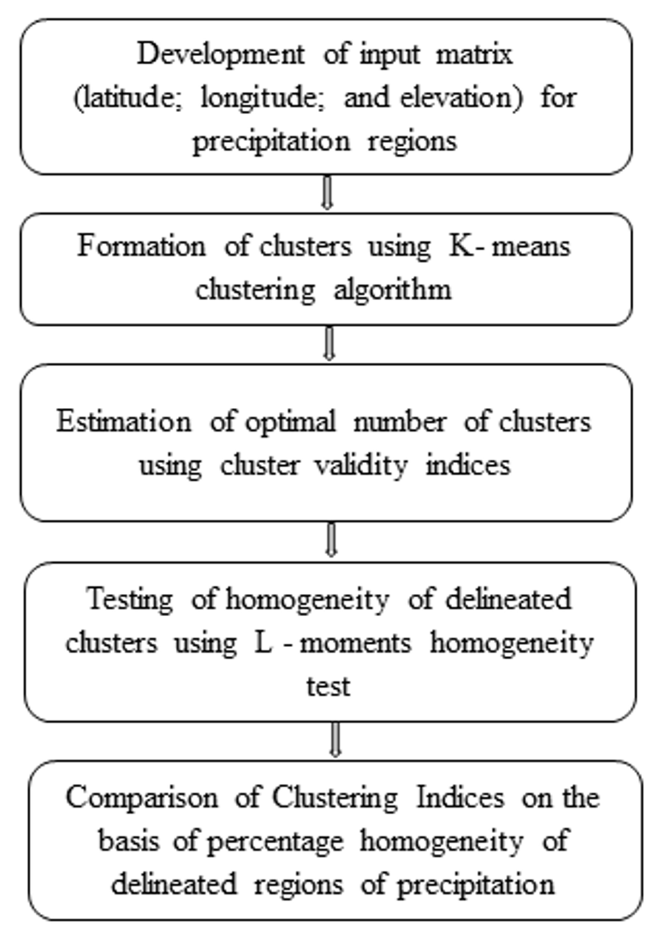
Efficient clustering algorithms aim at identifying homogeneous precipitation regions and discarding the irregularities present in the data distribution. In this section the three main steps are presented: (i) delineation of regions using k-means clustering, (ii) cluster validity indices (CVI), and (iii) validation of regions for homogeneity using L-moments ratio test, involved in the regionalization of precipitation zones. The framework for the delineation of precipitation regions is presented in Figure 1.

2.1. K–Means Clustering Algorithm

Clusters can be identified in a given set of data by determining a local minima solution through an iterative procedure, as McQueen [53] illustrated. This commonly used procedure is known as k-means clustering algorithm. This algorithm positions k centers amongst the data set and then assign the sites to its nearest center [54]. Those attributes having higher value have a more significant effect on the subsequent delineated clusters by k-means algorithm [9]. Therefore, the attributes are re-scaled to reduce the effect of their variances and relative magnitudes using,

$$x_{ji}^{\prime }=\frac{x_{ji}-{\mu }_j}{{\sigma }_j}$$

(1)

where, i and j represent attribute and site, respectively; $x_{ji}^{\prime }$ is the re-scaled value of $x_{ji}$; ${\mu }_j$ and ${\sigma }_j$ are the mean and the standard deviation, respectively for all sites.

Levine [55] proposed a procedure to cluster the data set by minimizing the distance of every site to each of the k cluster centers by re-assigning the attributes among the clusters. The objective function f is given as,

$$Minimize\left(f\right)={\displaystyle \sum _{k=1}^K}{\displaystyle \sum _{j=1}^n}{\displaystyle \sum _{i=1}^N}{\left\{d\left({x^{\prime }}_{ji}-c_j\right)\right\}}^2$$

(2)

where n-dimensional attribute space is denoted by n; N total number of features in the cluster and $c_j$ is the value of attribute j at the cluster’s centroid as defined in Equation (3); $d\left(\right)$ represents Euclidean distance measure; and k defines the number of centroids initialized beforehand.

$$c_j=\frac{{\displaystyle \sum _{i=1}^N}{x^{\prime }}_{ji}}{N}$$

(3)

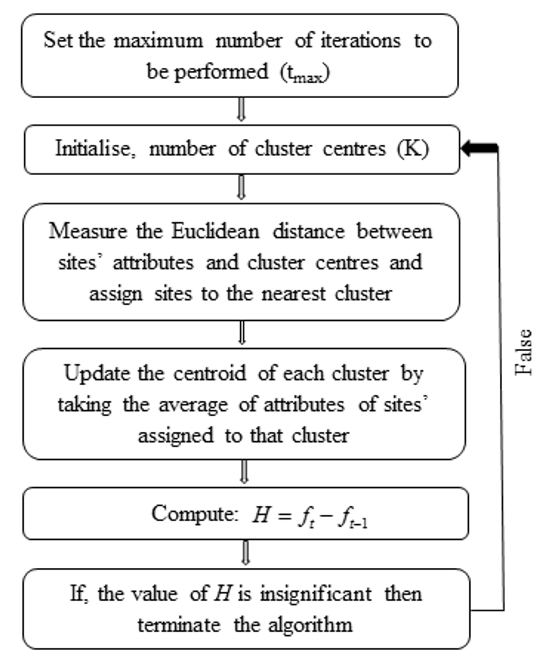
The steps involved in k-means clustering is shown in Figure 2. One of the major challenges in k-means clustering is to identify the initial guess for the number of clusters (k), before the procedure starts. This has a significant effect on the performance of the objective function in attaining the optimal number of clusters. Too many clusters will lead to outlining regions that do not exist, and too few will lead to poor differentiation among distinctly different neighborhoods. In this study, the number of clusters k is varied from 5 to 150 with an interval of 5. The CVIs are used to select the optimal value of k.

2.2. Cluster Validity Indices (CVIs)

Number of studies have used CVIs to obtain the optimal number of clusters (k) for a given attribute [20,27,44,45,46,47,48,49,50]. In this paper, the performances of 27 internal CVIs presented by Desgraupes [50] are compared for delineating the precipitation zones for two regions in Canada. The Dunn index is further classified into an additional 15 indices, resulting in a total of 42 internal CVIs. The goodness of the cluster is evaluated based on the information available from the data [56]. All the indices used in this study are presented in Appendix A, along with their mathematical form and selection criteria. The readers are referred to R programming based cluster package clusterCrit [50] for detailed information on the CVI.

2.3. L-Moments Homogeneity Test

Homogeneity tests are carried out to evaluate the statistical coherence of the clusters formed based on the attributes adopted for delineation of precipitation regions [57]. One of the broadly used procedure for testing the homogeneity of the clusters is L-moment homogeneity test [13]. The rationale of the homogeneity test is that population L-moment ratios is the same for the homogeneous cluster sites but different for their subset due to the variability in sampling. The advantages of the test are: (i) higher-order moments are estimated with minimum possible error; (ii) test can be performed with a wide range of distributions; (iii) test is robust to the data set; and (iv) results will be well interpreted since the value of L-moments vary between −1 and 1.

In this study, the weighted standard deviation is used to calculate sample coefficient of at-site L-variation (L-CV), which will be adopted as a heterogeneity measure [8]. Consider the cluster to be validated to have N number of sites and the length of rainfall dataset of site i to be $n_i$. The Equations (4)–(6) provide L-moment ratios for site i, L-CV ($l_i^2$), L-skewness ($l_i^3$), and L-kurtosis ($l_i^4$).

$$l_i^2=\frac{2\times {\displaystyle \sum _{j=2}^{n_i}}\left[p_j\left(\frac{j-1}{n_i-1}\right)\right]-{\displaystyle \sum _{j=1}^{n_i}}{p}_j}{{\displaystyle \sum _{j=1}^{n_i}}{p}_j}$$

(4)

$$l_i^3=\frac{6\times {\displaystyle \sum _{j=3}^{n_i}}\left[p_j\left\{{\displaystyle \prod _{k=1}^2}\left(\frac{j-k}{n_i-k}\right)\right\}\right]-6\times {\displaystyle \sum _{j=2}^{n_i}}\left[p_j\left(\frac{j-1}{n_i-1}\right)\right]+{\displaystyle \sum _{j=1}^{n_i}}{p}_j}{2\times {\displaystyle \sum _{j=2}^{n_i}}\left[p_j\left(\frac{j-1}{n_i-1}\right)\right]-{\displaystyle \sum _{j=1}^{n_i}}{p}_j}$$

(5)

$$l_i^4=\frac{20\times {\displaystyle \sum _{j=4}^{n_i}}\left[p_j\left\{{\displaystyle \prod _{k=1}^3}\left(\frac{j-k}{n_i-k}\right)\right\}\right]-30\times {\displaystyle \sum _{j=3}^{n_i}}\left[p_j\left\{{\displaystyle \prod _{k=1}^2}\left(\frac{j-k}{n_i-k}\right)\right\}\right]+12\times {\displaystyle \sum _{j=2}^{n_i}}\left[p_j\left(\frac{j-1}{n_i-1}\right)\right]-{\displaystyle \sum _{j=1}^{n_i}}{p}_j}{2\times {\displaystyle \sum _{j=2}^{n_i}}\left[p_j\left(\frac{j-1}{n_i-1}\right)\right]-{\displaystyle \sum _{j=1}^{n_i}}{p}_j}$$

(6)

where, $p_j$ is the $j^{th}$ observed precipitation measured at $i^{th}$ site. Therefore, the regional average L-CV ($l_i^R$), L-skewness ($l_3^R$), and L-kurtosis ($l_4^R$) are computed, as shown in Equations (7)–(9). The regional average mean ($l_1^R$) is set to 1 by scaling precipitation totals at each site by their mean values.

$$l_2^R=\frac{{\displaystyle \sum _{i=1}^N}{n}_i{l}_i^2}{{\displaystyle \sum _{i=1}^N}{n}_i}$$

(7)

$$l_3^R=\frac{{\displaystyle \sum _{i=1}^N}{n}_i{l}_i^3}{{\displaystyle \sum _{i=1}^N}{n}_i}$$

(8)

$$l_4^R=\frac{{\displaystyle \sum _{i=1}^N}{n}_i{l}_i^4}{{\displaystyle \sum _{i=1}^N}{n}_i}$$

(9)

Homogeneity of a cluster between site dispersion (D) is measured using,

$$D=\sqrt{\frac{{\displaystyle \sum _{i=1}^N}{n}_i{\left(l_i-l^R\right)}^2}{{\displaystyle \sum _{i=1}^N}{n}_i}}$$

(10)

The homogeneity of the clusters is compared using Kappa distribution derived from regional average L-moment ratios. In this study, 500 realizations are simulated from Kappa distribution for the study area. For each simulated regions, the value of D is determined. Let ${\mu }_D$ and ${\sigma }_D$ be the mean and standard deviation of 500 realizations, respectively. Then the heterogeneity measure for a cluster is defined as,

$$H=\frac{D-{\mu }_D}{{\sigma }_D}$$

(11)

If H < 1, then the cluster will be considered as “acceptably homogeneous”; else if $1\le H<2$, then the cluster will be regarded as “possibly homogeneous”; else if $H\ge 2$, then the delineated precipitation region is stated as “definitely heterogeneous”. For detailed information on L-moments the readers are referred to [13].

3. Case Study

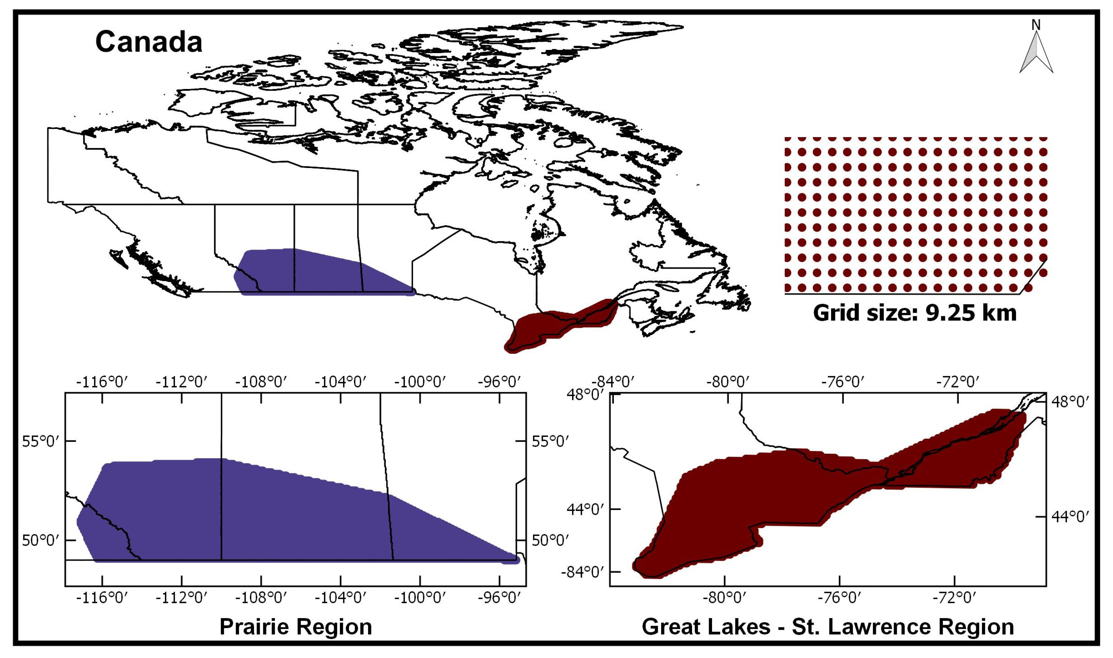
The methodology is employed in two climatic regions of Canada as shown in Figure 3, namely, the Prairies in Western Canada and the Great Lakes-St Lawrence lowlands (GL-SL) in Southern Ontario. These regions play a significant impact on agriculture, water infrastructure and economics of major cities such as Calgary, Edmonton, Regina, Winnipeg, Ottawa, Quebec, Montreal, and Toronto. The Prairie region largely depends on the frequency and the amount of precipitation. The precipitation in the region is mainly governed by large-scale atmospheric circulation and geophysical characteristics [10]. On the other hand, the climate of the GL-SL region is significantly affected due to the variations in the moisture content drawn from the large water bodies surrounding this region and the geophysical characteristics [58].

Prairie region is located at the southern border of Canada extending in three provinces (Alberta, Saskatchewan, and Manitoba) and in north-east extending up to the Rocky Mountains, as shown in Figure 3. The approximate extent of spatial boundaries varies from 49 to 54 degrees latitude and from −117 to −95 degrees longitude. Across this region, the distribution of precipitation varies along the provinces with maximum precipitation in Manitoba and minimum in the Saskatchewan [59]. The region is also characterized by seasonal precipitation variation [11]. The GL-SL region stretches from Southern Ontario to Quebec provinces and lies approximately between latitudes and longitudes of 42 to 48 degrees and −83 to −70 degrees respectively, as shown in Figure 3. The Great Lakes region covers Southern Ontario to the south of the Canadian Shield. The region experiences variable weather patterns due to the cold and dry air from the north, predominant winds and humid air blowing from the west and the Gulf of Mexico, respectively [60]. In the period from November to February, a cold air mass accumulates moisture by passing over the warm water bodies in the region and results in downwind precipitation [61]. In general, the precipitation in summer season in the Great Lakes is characterized by cloud bursts. In addition, the total annual precipitation varies across the region, with highest in the eastern part, i.e., St. Lawrence Valley sub-region experiences more annual precipitation than Great Lakes sub-region [11].

Data

Regionalization of precipitation regions requires good quality of spatial and temporal data. In the case of large-scale studies, the distribution of meteorological stations is not adequate for accurate estimation of regional parameters. In recent years, several studies have adopted gridded reanalysis or satellite data in the absence of historical data [11,16,62,63,64]. The major limitation of satellite data is the record length when compared to the reanalysis data. In this study, ANUSPLIN [65,66,67], a high-resolution gridded precipitation data is used for delineation of precipitation zones. This dataset has been used in several studies [11,68,69,70]. The grid map in Figure 3 shows the size of ANUSPLIN grid locations for both the regions. The data is approximately 300 arc second, and it contains 10810 and 3840 grid point locations within Prairie and GL-SL regions, respectively. It is to be noted that in Figure 3, due to the scale of the map, the grid location-based attributes appear to be a solid color. The data is ranging between years 1951–2005, for a record length of 55 years. The meta-data from the ANUSLIN is used to extract the location-based attributes for k-means clustering algorithm.

4. Results and Discussion

The daily precipitation series from ANUSPLIN point gridded data is aggregated to four seasons, namely winter (DJF), spring (MAM), summer (JJA), and autumn (SON). In this study, the location-based attributes such as elevation, latitude, and longitude are selected for delineation of precipitation regions. Asong et al. [10] and Irwin et al. [11] have also shown that the location-based attributes have a significant effect on the homogeneity of the regions. The Digital Elevation Model over the study regions is obtained from the Canadian Digital Elevation Data (CDED), which can be accessed from the Canadian GeoBase website (http://www.geobase.ca/). The elevation data from DEM is extracted at the latitude and longitude of the ANUSPLIN grid locations using Natural Neighborhood based interpolation method in ArcGIS 10.2.

4.1. Performance of the CVIs

The k-means clustering is adopted for the delineation of two large precipitation regions in Canada. The major limitations of this algorithm are the accuracy of the initial random centroids location and the identification of the optimal number of clusters, since it lacks theoretical background when compared to supervised algorithms [49]. Several studies have used an iterative process with initial random centroids to select the best clusters [11,15,71]. In this study, the k-means algorithm is executed for 50 iterations with varying initial random centroids, and the best cluster is selected for further analysis. Followed by, the identification of the optimal number of clusters is carried out using the CVIs. Finally, the optimal number of clusters is validated using the L-moments based homogeneity test. The regional percentage homogeneity represents the ratio of the total number of homogeneous clusters to the optimal number of clusters identified by CVI.

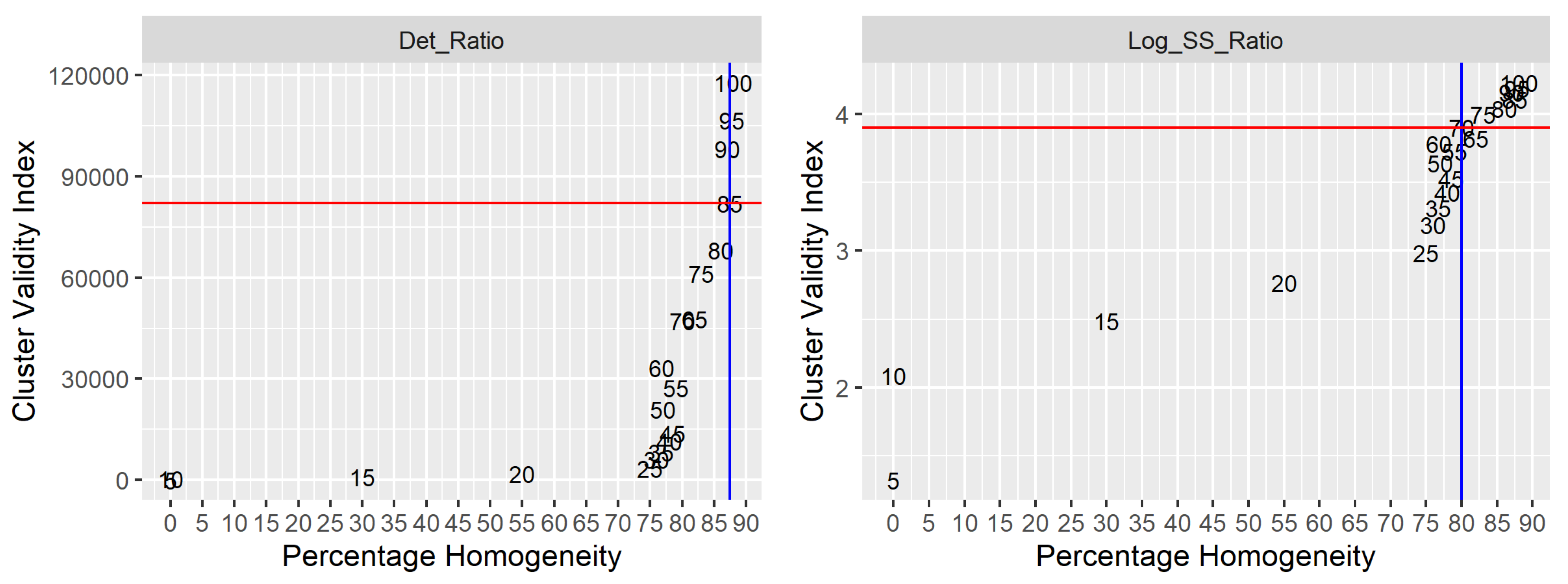
An illustrative example of the performance of two CVIs (Det-ratio and Log-SS-Ratio) is presented in Figure 4. The comparison is based on the percentage homogeneity, number of clusters and the CVI’s selection criteria. The Figure 4 describe: (i) CVI values (on y-axis); (ii) percentage homogeneity (on x-axis); (iii) the numerical in the panel indicate number of clusters resulting in the pair of CVI value and percentage homogeneity; (iv) horizontal y-intercept red line represents CVI’s ideal value based on the selection criteria presented in

Table A1. Cluster validity indices from clusterCrit R package developed by Desgraupes [50]. The clusterCrit name for each cluster index is presented in parenthesis. If the selection criteria is, minimum difference or maximum difference then, the clusters corresponding to the index value at which there is minimum slope or maximum slope difference versus number of clusters curve should be chosen.

Cluster Validity	Mathematical Equation	Selection
Index		Criteria
Ball-Hall
(Ball_Hall)	$C=\frac{1}{K}{\displaystyle \sum _{k=1}^K}\frac{1}{n_k}{\displaystyle {\displaystyle \sum _{i\in I_k}}}{∥M_i^{\left[k\right]}-G^{\left[k\right]}∥}^2$	Maximum
	where, C is the Cluster Validity Index; M${}^{\left[k\right]}$ is the matrix of attributes of kth cluster; G${}^{\left[k\right]}$ is the barycentre${}^{\#}$ of attributes in kth cluster; n${}_k$ is number of sites in kth cluster; K is the total number of clusters	Difference
Banfeld–Raftery
(Banfeld_Raftery)	$C={\displaystyle \sum _{k=1}^K}{n}_{k}log\left(\frac{1}{n_k}{\displaystyle \sum _{i\in I_k}}{∥M_i^{\left[k\right]}-G^{\left[k\right]}∥}^2\right)$	Minimum
C
(C_index)	$C=\frac{S_W-S_{min}}{S_{max}-S_{min}}$	Minimum
	where, N${}_W$ is the number of pairs of distinct sites in a cluster; S${}_W$ is the sum of N${}_W$ distances between all the pairs of sites inside each cluster; S${}_{min}$ is the sum of N${}_W$ smallest distances between all the pairs of sites in the entire dataset; S${}_{max}$ is the sum of N${}_W$ largest distances between all the pairs of sites in the entire dataset
$log\left(\frac{BGSS}{WGSS}\right)$
(Log_SS_Ratio)	$C=log\left(\frac{{\displaystyle \sum _{k=1}^K}{∥G^{\left[k\right]}-G∥}^2}{{\displaystyle \sum _{k=1}^K}{\displaystyle \sum _{i\in I_k}}{∥M_i^{{}^{\left[k\right]}}-G^{{}^{\left[k\right]}}∥}^2}\right)$	Minimum
		Difference
McClain–Rao
(McClain_Rao)	$C=\frac{N_B}{N_W}\frac{{\displaystyle \sum _{k=1}^K}{\displaystyle \sum _{\genfrac{}{}{0pt}{}{i,j\in I_k\hfill }{i<j\hfill }}}d\left(M_i,M_j\right)}{{\displaystyle \sum _{k<k^{\prime }}}{\displaystyle \sum _{\genfrac{}{}{0pt}{}{i\in I_k,j\in I_{k^{\prime }}\hfill }{i<j\hfill }}}d\left(M_i,M_j\right)}$	Minimum
	where, N${}_B$ is the number of pairs of sites which do not belong to the same cluster; M${}_i$ is the row matrix of ith site’s attributes; d() is the Euclidean distance between sites
PBM
(PBM)	$C={\left[\frac{1}{K}\times \frac{{\displaystyle \sum _{i=1}^N}d\left(M_i,G\right)}{{\displaystyle \sum _{k=1}^K}{\displaystyle \sum _{i\in I_k}}d\left(M_i,G^{\left[k\right]}\right)}\times \left\{{\displaystyle \underset{k<k^{\prime }}{max}}d\left(G^{\left[k\right]},G^{\left[k^{\prime }\right]}\right)\right\}\right]}^2$	Maximum
Point Biserial
(Point_Biserial)	$C=\left(\frac{{\displaystyle \sum _{k=1}^K}{\displaystyle \sum _{\begin{array}{c}i,j\in I_k\\ i<j\end{array}}}d\left(M_i,M_j\right)}{N_W}-\frac{{\displaystyle \sum _{k<k^{\prime }}}{\displaystyle \sum _{\begin{array}{c}i\in I_k,j\in I_{k^{\prime }}\\ i<j\end{array}}}d\left(M_i,M_j\right)}{N_B}\right)\times \frac{\sqrt{N_W{N}_B}}{N_T}$	Maximum
	where, N${}_T$ is the total number of pairs of distinct sites in the dataset
Calinski–Harabasz
(Calinski_Harabasz)	$C=\frac{N-K}{K-1}\left(\frac{{\displaystyle \sum _{k=1}^K}{∥G^{\left[k\right]}-G∥}^2}{{\displaystyle \sum _{k=1}^K}{\displaystyle \sum _{i\in I_k}}{∥M_i^{\left[k\right]}-G^{\left[k\right]}∥}^2}\right)$	Maximum
Davies–Bouldin
(Davies_Bouldin)	$C=\frac{1}{K}{\displaystyle \sum _{k=1}^K}{\displaystyle \underset{k^{\prime }\ne k}{max}}\left(\frac{\left(\frac{1}{n_k}{\displaystyle \sum _{i\in I_k}}∥M_i^{\left[k\right]}-G^{\left[k\right]}∥\right)+\left(\frac{1}{n_{k^{\prime }}}{\displaystyle \sum _{i\in I_{k^{\prime }}}}∥M_i^{\left[k^{\prime }\right]}-G^{\left[k^{\prime }\right]}∥\right)}{∥G^{\left[k\right]}-G^{\left[k^{\prime }\right]}∥}\right)$	Minimum
$\frac{\left|T\right|}{\left|W\right|}$
(Det_Ratio)	$C=\frac{det\left({}^{t}XX\right)}{det\left({\displaystyle \sum _{k=1}^K}{}^t{X}^{\left[k\right]}{X}^{\left[k\right]}\right)}$	Minimum
	where, X is the matrix formed by centred vectors $v_j=V_j-{\mu }_j$ for entire dataset; X${}^{\left[k\right]}$ is the matrix formed by centred vectors $v_j^{\left\{k\right\}}=V_j^{\left\{k\right\}}-{\mu }_j^{\left\{k\right\}}$ for each cluster k; V${}_j$ is the jth observed attribute; ${\mu }_j$ is the barycentre${}^{\#}$ of jth observed attribute	Difference
Dunn
(Dunn)	$C=\frac{{\displaystyle \underset{k\ne k^{\prime }}{min\left({\displaystyle \underset{\genfrac{}{}{0pt}{}{i\in I_k\hfill }{j\in I_{{}_{k^{\prime }}}\hfill }}{min}}∥M_i^{\left[k\right]}-M_j^{\left[k^{\prime }\right]}∥\right)}}}{{\displaystyle \underset{1\le k\le K}{max\left({\displaystyle \underset{i,j\in I_k}{max}}∥M_i^{\left[k\right]}-M_j^{\left[k\right]}∥\right)}}}$	Maximum
Dunn Generalized (1, 1)
(GDI11)	$C=\frac{{min}_{k\ne k^{\prime }}\left({\displaystyle \underset{\begin{array}{c}i\in I_k\\ j\in I_{k^{\prime }}\end{array}}{min}}d\left(M_i,M_j\right)\right)}{{max}_k\left({\displaystyle \underset{\begin{array}{c}i,j\in I_k\\ i\ne j\end{array}}{max}}d\left(M_i,M_j\right)\right)}$	Maximum
Dunn Generalized (1, 2)
(GDI12)	$C=\frac{{min}_{k\ne k^{\prime }}\left({\displaystyle \underset{\begin{array}{c}i\in I_k\\ j\in I_{k^{\prime }}\end{array}}{min}}d\left(M_i,M_j\right)\right)}{{max}_k\left(\frac{1}{n_k\left(n_k-1\right)}{\displaystyle \sum _{\begin{array}{c}i,j\in I_k\\ i\ne j\end{array}}}d\left(M_i,M_j\right)\right)}$	Maximum
Dunn Generalized (1, 3)
(GDI13)	$C=\frac{{min}_{k\ne k^{\prime }}\left({\displaystyle \underset{\begin{array}{c}i\in I_k\\ j\in I_{k^{\prime }}\end{array}}{min}}d\left(M_i,M_j\right)\right)}{{max}_k\left(\frac{2}{n_k}{\displaystyle \sum _{i\in I_k}}d\left(M_i,G^{\left\{k\right\}}\right)\right)}$	Maximum
Dunn Generalized (2, 1)
(GDI21)	$C=\frac{{min}_{k\ne k^{\prime }}\left({\displaystyle \underset{\begin{array}{c}i\in I_k\\ j\in I_{k^{\prime }}\end{array}}{max}}d\left(M_i,M_j\right)\right)}{{max}_k\left({\displaystyle \underset{\begin{array}{c}i,j\in I_k\\ i\ne j\end{array}}{max}}d\left(M_i,M_j\right)\right)}$	Maximum
Dunn Generalized (2, 2)
(GDI22)	$C=\frac{{min}_{k\ne k^{\prime }}\left({\displaystyle \underset{\begin{array}{c}i\in I_k\\ j\in I_{k^{\prime }}\end{array}}{max}}d\left(M_i,M_j\right)\right)}{{max}_k\left(\frac{1}{n_k\left(n_k-1\right)}{\displaystyle \sum _{\begin{array}{c}i,j\in I_k\\ vci\ne j\end{array}}}d\left(M_i,M_j\right)\right)}$	Maximum
Dunn Generalized (2, 3)
(GDI23)	$C=\frac{{min}_{k\ne k^{\prime }}\left({\displaystyle \underset{\begin{array}{c}i\in I_k\\ j\in I_{k^{\prime }}\end{array}}{max}}d\left(M_i,M_j\right)\right)}{{max}_k\left(\frac{2}{n_k}{\displaystyle \sum _{i\in I_k}}d\left(M_i,G^{\left\{k\right\}}\right)\right)}$	Maximum
Dunn Generalized (3, 1)
(GDI31)	$C=\frac{{min}_{k\ne k^{\prime }}\left(\frac{1}{n_k{n}_{k^{\prime }}}{\displaystyle \sum _{\begin{array}{c}i\in I_k\\ j\in I_{k^{\prime }}\end{array}}}d\left(M_i,M_j\right)\right)}{{max}_k\left({\displaystyle \underset{\begin{array}{c}i,j\in I_k\\ i\ne j\end{array}}{max}}d\left(M_i,M_j\right)\right)}$	Maximum
Dunn Generalized (3, 2)
(GDI32)	$C=\frac{{min}_{k\ne k^{\prime }}\left(\frac{1}{n_k{n}_{k^{\prime }}}{\displaystyle \sum _{\begin{array}{c}i\in I_k\\ j\in I_{k^{\prime }}\end{array}}}d\left(M_i,M_j\right)\right)}{{max}_k\left(\frac{1}{n_k\left(n_k-1\right)}{\displaystyle \sum _{\begin{array}{c}i,j\in I_k\\ i\ne j\end{array}}}d\left(M_i,M_j\right)\right)}$	Maximum
Dunn Generalized (3, 3)
(GDI33)	$C=\frac{{min}_{k\ne k^{\prime }}\left({\displaystyle \underset{\genfrac{}{}{0pt}{}{i\in I_k\hfill }{j\in I_{k^{\prime }}\hfill }}{max}}d\left(M_i,M_j\right)\right)}{{max}_k\left(\frac{2}{n_k}{\displaystyle \sum _{i\in I_k}}d\left(M_i,G^{\left[k\right]}\right)\right)}$	Maximum
Dunn Generalized (4, 1)
(GDI41)	$C=\frac{{min}_{k\ne k^{\prime }}d\left(G^{\left[k\right]},G^{\left[k^{\prime }\right]}\right)}{{max}_k\left({\displaystyle \underset{\genfrac{}{}{0pt}{}{i,j\in I_k\hfill }{i\ne j\hfill }}{max}}d\left(M_i,M_j\right)\right)}$	Maximum
Dunn Generalized (4, 2)
(GDI42)	$C=\frac{{min}_{k\ne k^{\prime }}d\left(G^{\left\{k\right\}},G^{\left\{k^{\prime }\right\}}\right)}{{max}_k\left(\frac{1}{n_k\left(n_k-1\right)}{\displaystyle \sum _{\genfrac{}{}{0pt}{}{i,j\in I_k\hfill }{i\ne j\hfill }}}d\left(M_i,M_j\right)\right)}$	Maximum
Dunn Generalized (4, 3)
(GDI43)	$C=\frac{{min}_{k\ne k^{\prime }}d\left(G^{\left\{k\right\}},G^{\left\{k^{\prime }\right\}}\right)}{{max}_k\left(\frac{2}{n_k}{\displaystyle \sum _{i\in I_k}}d\left(M_i,G^{\left\{k\right\}}\right)\right)}$	Maximum
Dunn Generalized (5, 1)
(GDI51)	$C=\frac{{min}_{k\ne k^{\prime }}\left(\frac{1}{n_k+n_{k^{\prime }}}\left({\displaystyle \sum _{i\in I_k}}d\left(M_i,G^{\left\{k\right\}}\right)+{\displaystyle \sum _{j\in I_{k^{\prime }}}}d\left(M_j,G^{\left\{k^{\prime }\right\}}\right)\right)\right)}{{max}_k\left({\displaystyle \underset{\genfrac{}{}{0pt}{}{i,j\in I_k\hfill }{i\ne j\hfill }}{max}}d\left(M_i,M_j\right)\right)}$	Maximum
Dunn Generalized (5, 2)
(GDI52)	$C=\frac{{min}_{k\ne k^{\prime }}\left(\frac{1}{n_k+n_{k^{\prime }}}\left({\displaystyle \sum _{i\in I_k}}d\left(M_i,G^{\left\{k\right\}}\right)+{\displaystyle \sum _{j\in I_{k^{\prime }}}}d\left(M_j,G^{\left\{k^{\prime }\right\}}\right)\right)\right)}{{max}_k\left(\frac{1}{n_k\left(n_k-1\right)}{\displaystyle \sum _{\genfrac{}{}{0pt}{}{i,j\in I_k\hfill }{i\ne j\hfill }}}d\left(M_i,M_j\right)\right)}$	Maximum
Dunn Generalized (5, 3)
(GDI53)	$C=\frac{{min}_{k\ne k^{\prime }}\left(\frac{1}{n_k+n_{k^{\prime }}}\left({\displaystyle \sum _{i\in I_k}}d\left(M_i,G^{\left\{k\right\}}\right)+{\displaystyle \sum _{j\in I_{k^{\prime }}}}d\left(M_j,G^{\left\{k^{\prime }\right\}}\right)\right)\right)}{{max}_k\left(\frac{2}{n_k}{\displaystyle \sum _{i\in I_k}}d\left(M_i,G^{\left\{k\right\}}\right)\right)}$	Maximum
Gamma
(Gamma)	$C=\Gamma =\frac{s^{+}-s^{-}}{s^{+}+s^{-}}$	Maximum
	where, $s^{+}$ is the number of pairs of sites which are not in same cluster and whose distance is less than those which are in same cluster; $s^{-}$ is the number of pairs which are in same cluster and whose distance is more than those which are in same cluster
G+
(G_plus)	$C=\frac{2s^{-}}{N_T\left(N_T-1\right)}$	Minimum
$k^2$
(Ksq_DetW)	$C=K^{2}det\left({\displaystyle \sum _{k=1}^K}{}^t{X}^{\left\{k\right\}}{X}^{\left\{k\right\}}\right)$	Maximum
	where, det() is the determinant of the matrix	Difference
Wemmet - Gan arski
(Wemmet _Gancarski)	$C=\frac{1}{N}{\displaystyle \sum _{k=1}^K}max\left\{0,n_k-{\displaystyle \sum _{i\in I_k}}\left(\frac{∥M_i-G^{\left\{k\right\}}∥}{{\displaystyle \underset{k^{\prime }\ne k}{min}}∥M_i-G^{\left\{k^{\prime }\right\}}∥}\right)\right\}$	Maximum
$log\left(\frac{\left|T\right|}{\left|W\right|}\right)$
(Log_Det_Ratio)	$C=Nlog\left(\frac{det\left({}^{t}XX\right)}{det\left({\displaystyle \sum _{k=1}^K}{}^t{X}^{\left\{k\right\}}{X}^{\left\{k\right\}}\right)}\right)$	Minimum
		Difference
Ratkowsky–Lance
(Ratkowsky_Lance)	$C=\sqrt{\frac{\frac{1}{p}{\displaystyle \sum _{j=1}^p}\frac{{\displaystyle \sum _{k=1}^K}{n}_k{\left({\mu }_j^{\left\{k\right\}}-{\mu }_j\right)}^2}{{\displaystyle \sum _{i=1}^N}{\left(a_{ij}-{\mu }_j\right)}^2}}{K}}$	Maximum
	where, p is the total number of attributes; a${}_{ij}$ is the jth attribute of ith site
Ray–Turi
(Ray_Turi)	$C=\frac{1}{N}\times \frac{{\displaystyle \sum _{k=1}^K}{\displaystyle \sum _{i\in I_k}}{∥M_i^{\left\{k\right\}}-G^{\left\{k\right\}}∥}^2}{{\displaystyle \underset{k<k^{\prime }}{min{∥G^{\left\{k\right\}}-G^{\left\{k^{\prime }\right\}}∥}^2}}}$	Minimum
Scott–Symons
(Scott_Symons)	$C={\displaystyle \sum _{k=1}^K}{n}_{k}logdet\left(\frac{{}^t{X}^{\left[k\right]}{X}^{\left[k\right]}}{n_k}\right)$	Minimum
SD [Scat]
(SD_Scat)	$\frac{\frac{1}{K}{\displaystyle \sum _{k=1}^K}∥\left(Var\left(V_1^{\left\{k\right\}}\right),\dots \dots ,Var\left(V_p^{\left\{k\right\}}\right)\right)∥}{∥\left(Var\left(V_1\right),\dots \dots ,Var\left(V_p\right)\right)∥}$	Minimum
	where, Var() of the attribute
SD [Dis]
(SD_Dis)	$\frac{{\displaystyle \underset{k=k^{\prime }}{max}}{∥G^{\left\{k\right\}}-G^{\left\{k^{\prime }\right\}}∥}^2}{{\displaystyle \underset{k=k^{\prime }}{min}}{∥G^{\left\{k\right\}}-G^{\left\{k^{\prime }\right\}}∥}^2}{\displaystyle \sum _{k=1}^K}\frac{1}{{\displaystyle \sum _{\genfrac{}{}{0pt}{}{k^{\prime }\ne 1\hfill }{k^{\prime }\ne k\hfill }}^K}{∥G^{\left\{k\right\}}-G^{\left\{k^{\prime }\right\}}∥}^2}$	Minimum
S-Dbw
(S_Dbw)	$\begin{array}{c}C=\frac{\frac{1}{K}{\displaystyle \sum _{k=1}^K}∥Var\left(V_1^{\left\{k\right\}}\right),\dots ..,Var\left(V_p^{\left\{k\right\}}\right)∥}{∥Var\left(V_1\right),\dots ,Var\left(V_p\right)∥}\hfill \\ +\frac{2}{K\left(K-1\right)}{\displaystyle \sum _{k<k^{\prime }}}\frac{{\gamma }_{k{k}^{\prime }}\left(H_{k{k}^{\prime }}\right)}{max\left({\gamma }_{k{k}^{\prime }}\left(G^{\left\{k\right\}}\right),{\gamma }_{k{k}^{\prime }}\left(G^{\left\{k^{\prime }\right\}}\right)\right)}\hfill \end{array}$
	where, H${}_{kk\prime }$ is the mid-point of G${}^k$ and G ${}^{k^{\prime }}$; ${\gamma }_{k{k}^{\prime }}$() is the total number of sites in these kth and k${}^{{}^{\prime }th}$ clusters whose distance to the given point is less than
	$\frac{1}{K}\sqrt{{\displaystyle \sum _{k=1}^K}∥Var\left(V_1^{\left\{k\right\}}\right),\dots ..,Var\left(V_p^{\left\{k\right\}}\right)∥}$	Minimum
Silhouette
(Silhouette)	$C=\frac{1}{K}{\displaystyle \sum _{k=1}^K}\left(\frac{1}{n_k}{\displaystyle \sum _{i\in I_k}}\frac{\frac{1}{n_{k^{\prime }}}{\displaystyle \sum _{i^{\prime }\in I_{k^{\prime }}}}d\left(M_i,M_{i^{\prime }}\right)-\frac{1}{n_k-1}{\displaystyle \sum _{\genfrac{}{}{0pt}{}{i^{\prime }\in I_k\hfill }{i\ne i^{\prime }\hfill }}}d\left(M_i,M_{i^{\prime }}\right)}{max\left(\frac{1}{n_{k^{\prime }}}{\displaystyle \sum _{i^{\prime }\in I_{k^{\prime }}}}d\left(M_i,M_{i^{\prime }}\right),\frac{1}{n_k-1}{\displaystyle \sum _{\genfrac{}{}{0pt}{}{i^{\prime }\in I_k\hfill }{i\ne i^{\prime }\hfill }}}d\left(M_i,M_{i^{\prime }}\right)\right)}\right)$	Maximum
Tr(W)
(Trace_W)	$C=Tr\left({\displaystyle \sum _{k=1}^K}{\displaystyle \sum _{i\in I_k}}{∥M_i^{\left\{k\right\}}-G^{\left\{k\right\}}∥}^2\right)$	Maximum
	where, Tr() is the trace of the matrix	Difference
Tr(W-1B)
(Trace_WiB)	$C=Tr\left\{{\left({\displaystyle \sum _{k=1}^K}{}^t{X}^{\left\{k\right\}}{X}^{\left\{k\right\}}\right)}^{-1}.\left({}^{t}BB\right)\right\}$	Maximum
	where, B is the matrix formed in rows by the vectors ${\mu }^{\left\{k\right\}}-\mu$ where $1\le k\le K$	Difference
Xie–Beni
(Xie_Beni)	$C=\frac{1}{N}\frac{{\displaystyle \sum _{k=1}^K}{\displaystyle \sum _{i\in I_k}}{∥M_i^{\left\{k\right\}}-G^{\left\{k\right\}}∥}^2}{{\displaystyle \underset{k<k^{\prime }}{min}}\left({\displaystyle \underset{\genfrac{}{}{0pt}{}{i\in I_k\hfill }{j\in I_{k^{\prime }}\hfill }}{min}}d\left(M_i,M_j\right)\right)}$	Minimum
Tau
(Tau)	$C=\frac{s^{+}-s^{-}}{\sqrt{N_B{N}_W\left(\frac{N_T\left(N_T-1\right)}{2}\right)}}$	Maximum

; (v) vertical x-intercept blue line represents the value of percentage homogeneity with respect to the CVI’s ideal value in (iv). In Figure 4, the CVI value, number of clusters, and percentage homogeneity corresponding to the CVI’s ideal value (red lines) are (82003, 85, 87.5%) and (3.900, 70, 80%) for Det-Ratio and Log-SS-Ratio, respectively. The selection of CVI is based on the higher value of percentage homogeneity among the CVIs. In case, if the CVIs have similar/equal percentage homogeneity, then the CVI with the lower number of clusters is selected. In the example illustrated, it is evident that the Det-Ratio is able to obtain a higher value of percentage homogeneity (87.5%) when compared to Log-SS-Ratio which is (72%) and hence the Det-Ratio based CVI is selected. Similarly, the relative performance of several CVIs can be assessed based on the above selection procedure.

4.2. Application to Canadian Regions

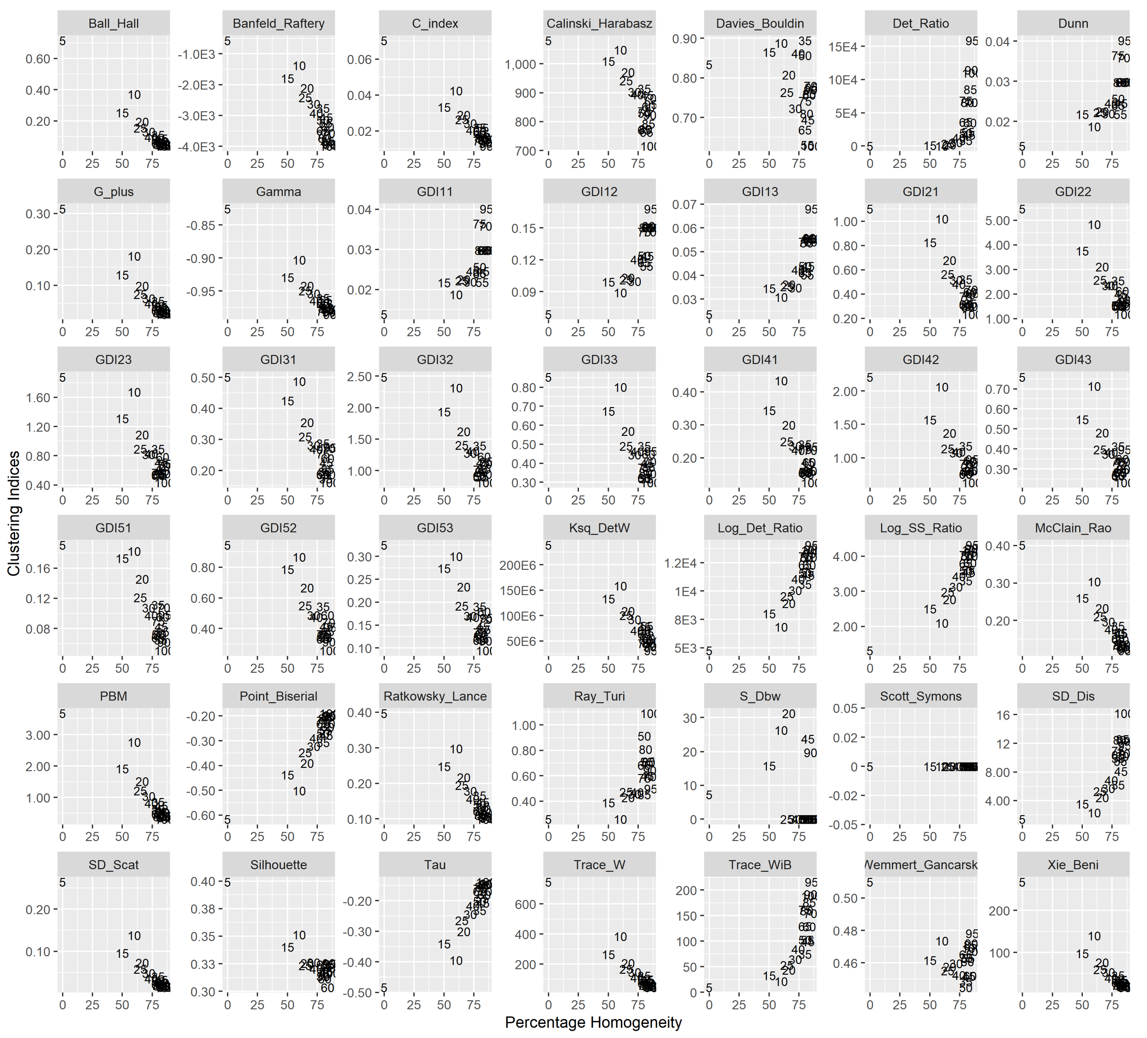
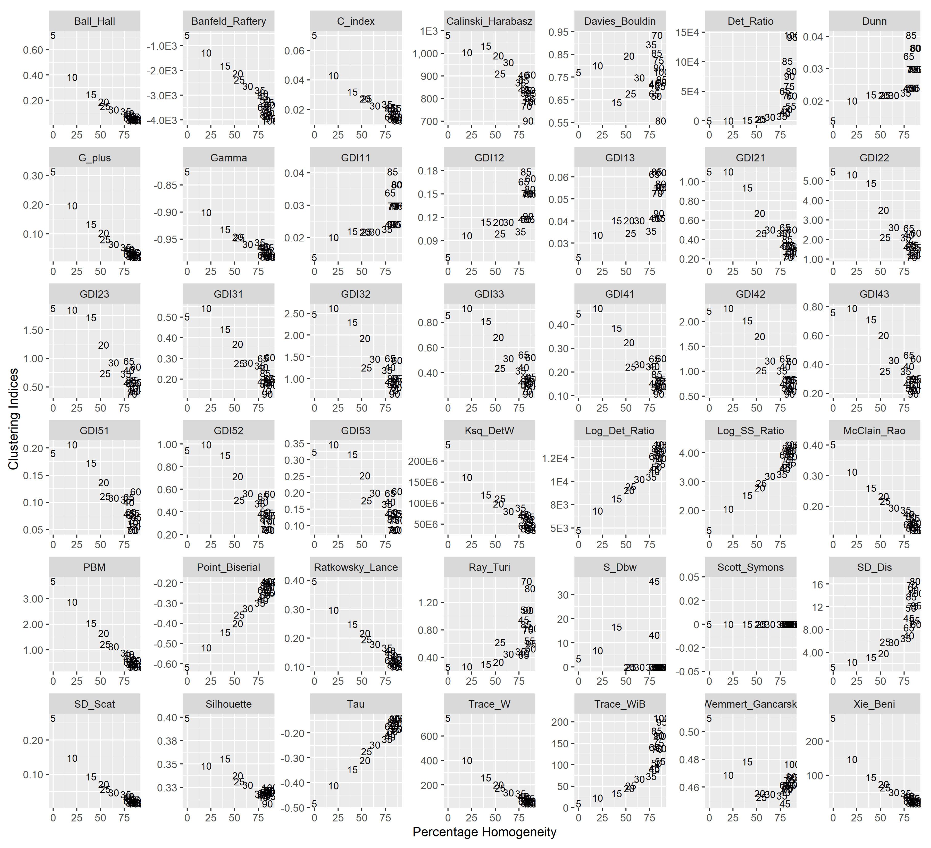
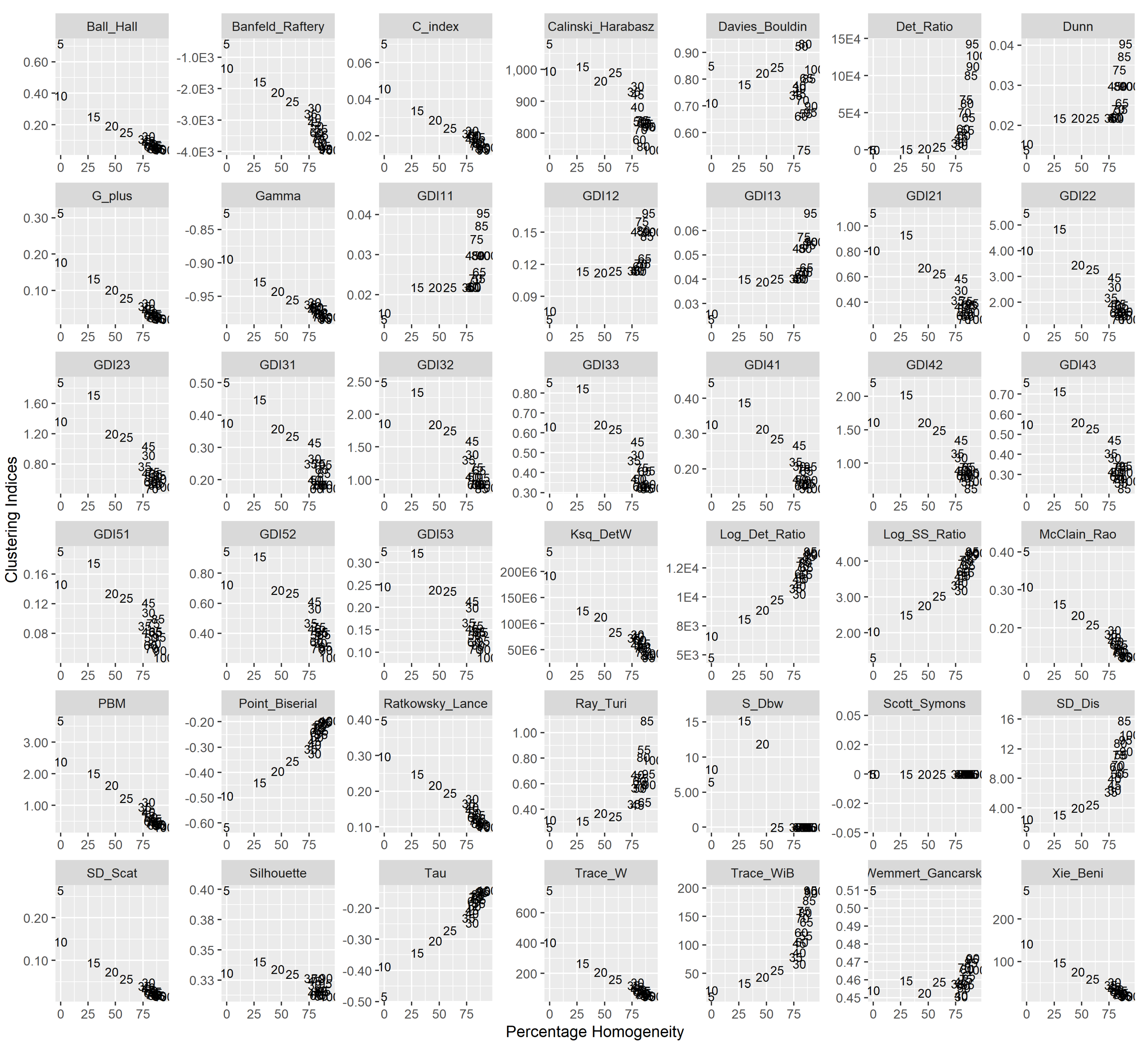
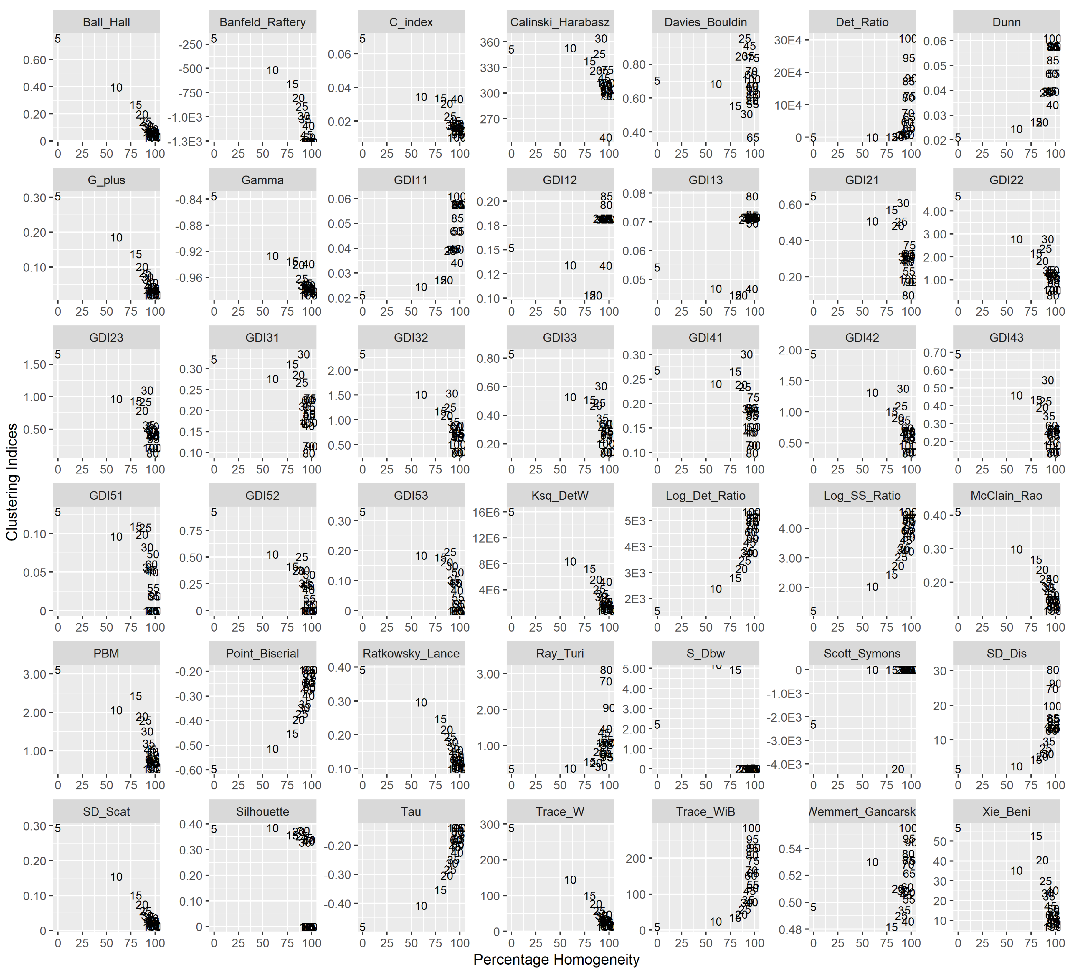
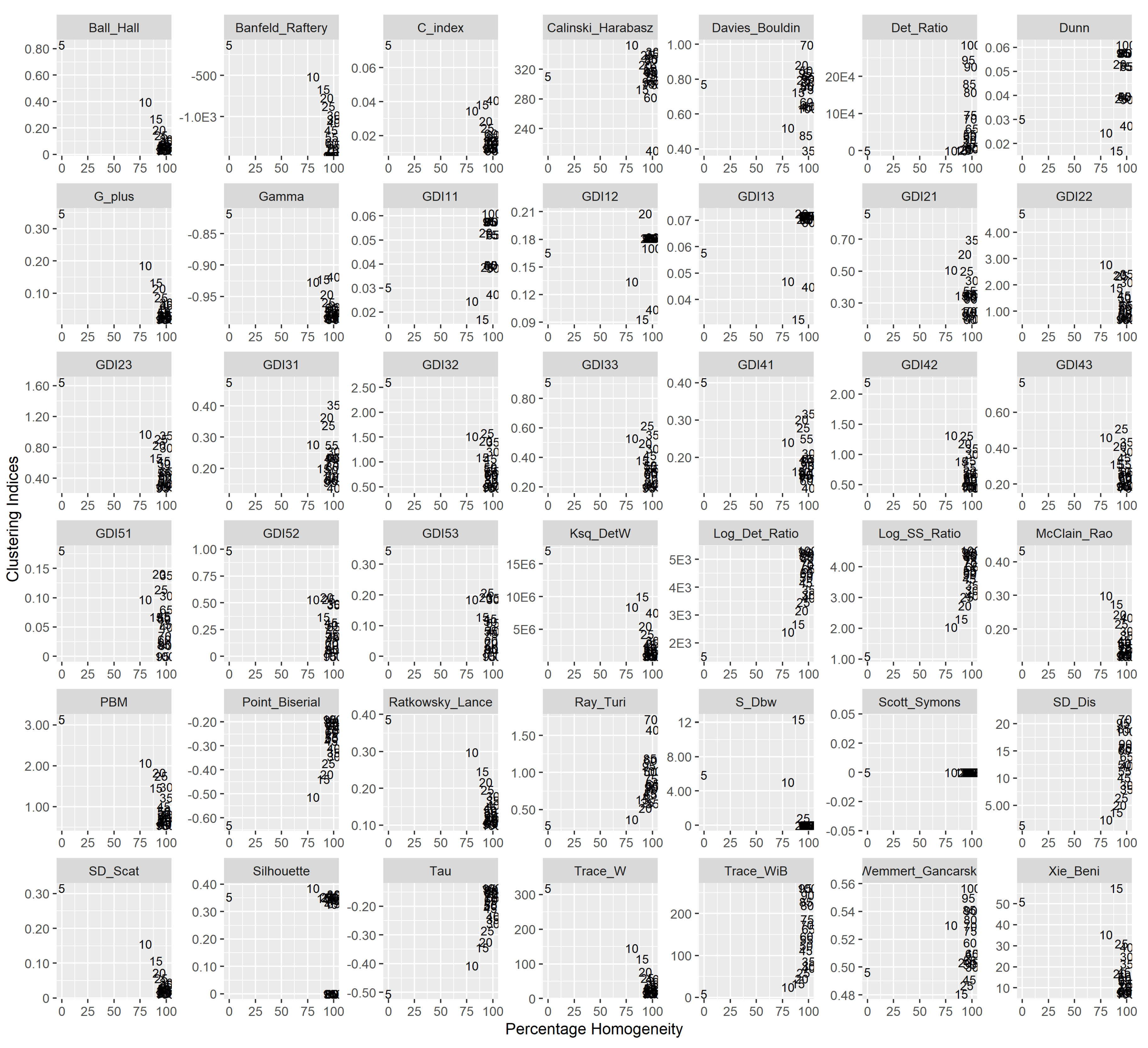
The performance of the 42 CVIs for four seasons in the two Canadian Regions are presented in Figure 5, Figure 6, Figure 7, Figure 8, Figure 9, Figure 10, Figure 11 and Figure 12. The number of clusters is varied from 5 to 150 at an interval of 5, and the ideal number of clusters is selected based on the CVI selection criteria as presented in Table A1. For brevity, the results for the number of clusters is limited to 100, since no significant changes were observed beyond this cluster number. In addition, the results are also compared with the performance of the empirical formula. The number of clusters formed using empirical formula is 27 and 22 for the Prairie and GL-SL region, respectively. It is to be noted that Irwin et al. [11] found that the optimal number of clusters is significantly different from empirical formula for each season and both the regions of Canada. The results for each region is presented as follows:

4.2.1. Prairie Region

The 10810 sites of Prairie region were regionalized into 27 clusters using the empirical formula, thus giving the percentage homogeneity in, (i) Winter season—81%, (ii) Spring season—78%, (iii) Summer season—78%, and (iv) Autumn season—76%. The variation of percentage of homogeneity for each CVI and the number of clusters are presented in Figure 5, Figure 6, Figure 7 and Figure 8. The coordinates of the same are marked with the number of clusters which divided the region. Out of 42 CVIs, 14 of them outperform in comparison to empirical formula in all the seasons. The selected 14 indices along with the best number of clusters and their corresponding percentage homogeneity are listed in

Table 1. Number of clusters and their corresponding percentage homogeneity values for the selected CVI for each season in Prairie region.

Clustering Indices	Winter Season		Spring Season		Summer Season		Autumn Season
	#Clusters ${}^1$	%Hom ${}^2$	#Clusters ${}^1$	%Hom ${}^2$	#Clusters ${}^1$	%Hom ${}^2$	#Clusters ${}^1$	%Hom ${}^2$
Banfeld_Raftery	100	89.48	100	85.26	100	88.42	100	89.47
C_index	100	89.48	100	85.26	100	88.42	95	88.89
Det_Ratio	85	87.50	80	86.67	85	87.50	95	88.89
Dunn	55	86.00	100	85.26	100	88.42	95	88.89
G_plus	95	88.89	100	85.26	100	88.42	100	89.47
GDI11	55	86.00	100	85.26	100	88.42	95	88.89
GDI12	80	88.00	90	84.71	100	88.42	95	88.89
GDI13	100	89.48	95	85.56	100	88.42	95	88.89
McClain_Rao	100	89.48	100	85.26	100	88.42	95	88.89
Point_Biserial	95	88.89	100	85.26	100	88.42	100	89.48
SD_Scat	100	89.48	100	85.26	100	88.42	100	89.48
Tau	95	88.89	100	85.26	100	88.42	100	89.48
Trace_WiB	95	88.89	75	84.29	70	84.61	55	84.00
Xie_Beni	100	89.48	100	85.26	100	88.42	95	88.89

${}^1$# Clusters: Number of Clusters; ${}^2$% Hom: Percentage Homogeneity.

. The maximum percentage homogeneity determined for each season is:

• Winter season: Banfeld–Raftery index, C index, Dunn generalized 1, 3 index, McClain–Rao index, SD [Scat] index, and Xie–Beni index suggest k = 100 as optimal partition giving 89 homogeneous regions amongst them. The Dunn index and their modifications (GDI11) provide a similar percentage of homogeneity (86%) with larger clusters (55 numbers).
• Spring Season: $\frac{\left|T\right|}{\left|W\right|}$ ratio index found to be the best in delineation of the region in 80 clusters out of which 69 clusters are homogeneous.
• Summer season: All the indices except, $\frac{\left|T\right|}{\left|W\right|}$ index and Tr(W-1B) index recommend to divide the area in 100 clusters, which further give 88 homogeneous ones.
• Autumn season: Banfeld–Raftery index, G + index, Point–Biserial index, SD [Scat] index, and Tau index regionalize the area in 100 clusters resulting in 89 homogeneous ones. The Trace_WiB cluster index has resulted in the lower number of clusters (55) with homogeneity of 84%.

In addition, with a notable comparison between seasons, seven CVIs delineate the region with highest percentage homogeneity for the Autumn season, ten indices regionalize with best percentage homogeneity in the Winter season, and three indices provide similar results for both winter and autumn seasons as shown in

Table 2. Season-wise comparison of cluster validity indices.

Cluster Validity Index	Prairies Region	Great Lakes-St. Lawrence Lowlands Region
Banfeld_Raftery	Winter and	Autumn Season
	Autumn Season
C_index	Winter Season	Autumn Season
Det_Ratio	Autumn Season	Autumn Season
Davies_Bouldin	-	Autumn Season
Dunn	Autumn Season	Autumn Season
G_plus	Autumn Season	Autumn Season
GDI11	Autumn Season	Autumn Season
GDI12	Autumn Season	Autumn Season
GDI13	Winter Season	Autumn Season
McClain_Rao	Winter Season	Autumn Season
Point_Biserial	Autumn Season	Autumn Season
SD_Scat	Winter and	Autumn Season
	Autumn Season
Tau	Autumn Season	Autumn Season
Trace_WiB	Winter Season	Autumn Season
Xie_Beni	Winter Season	Autumn Season

. In addition, it is observed that among the selected best indices, the Dunn and Trace_WiB index provides a smaller number of clusters when compared to other indices in Winter and Autumn seasons.

4.2.2. Great Lakes-St. Lawrence Lowlands (GL-SL) Region

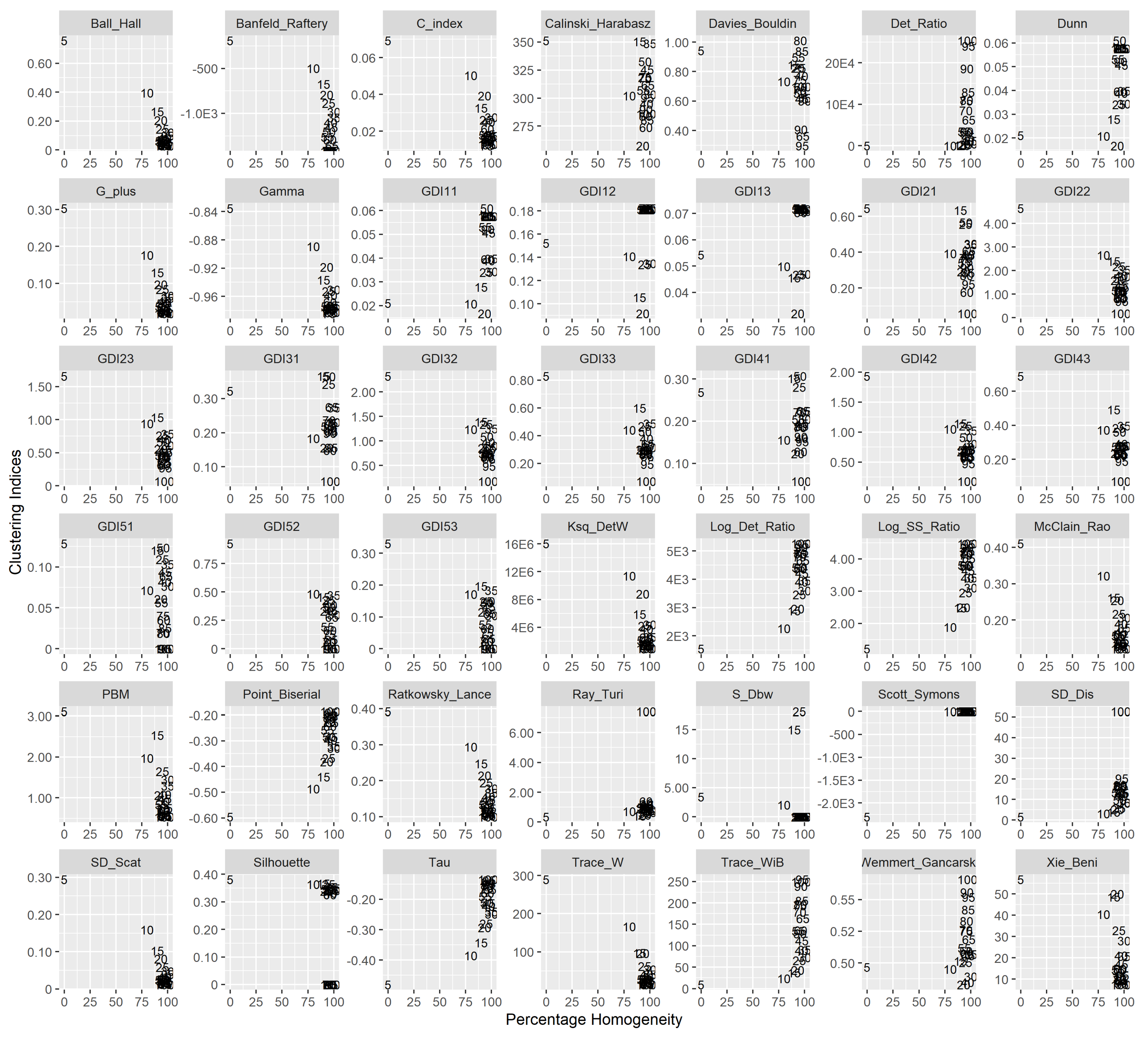
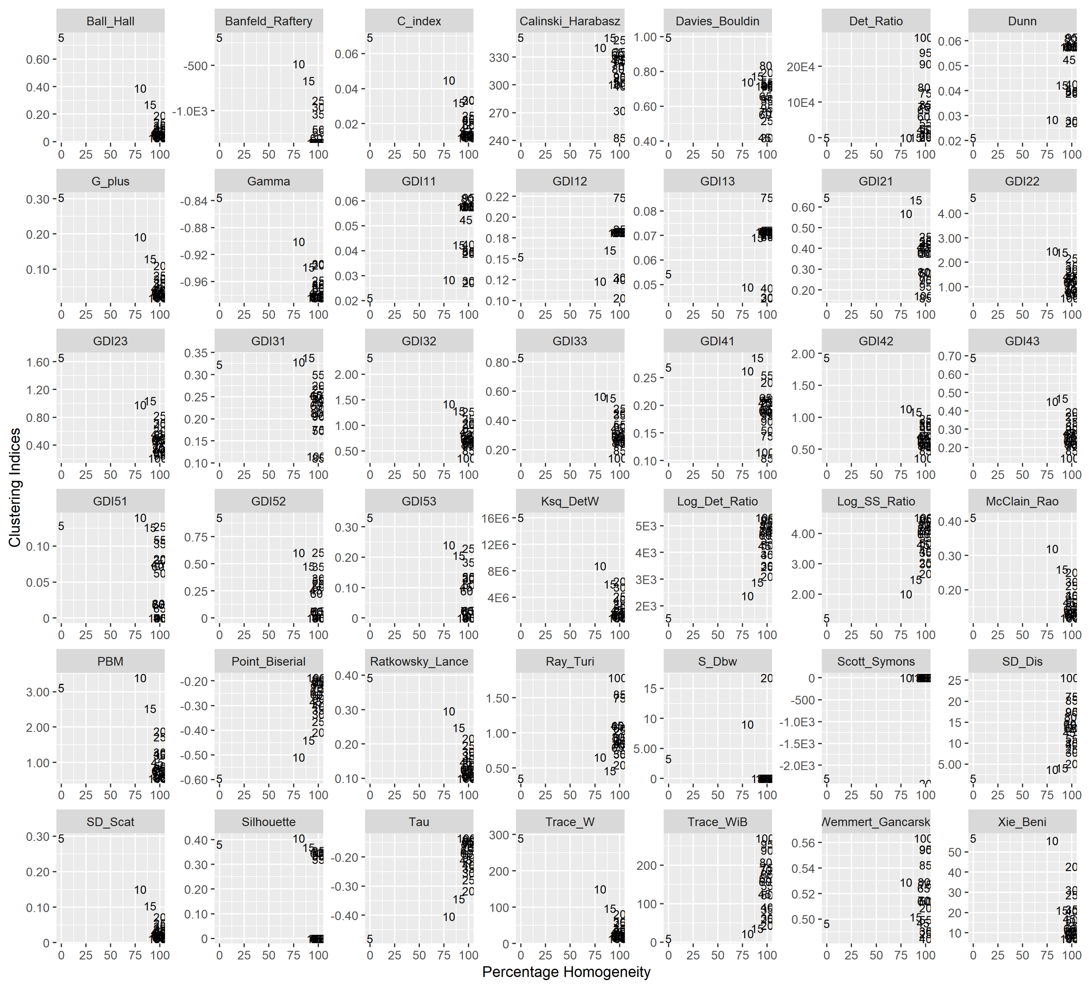
Great Lakes-St. Lawrence lowlands region is comprised of 3840 sites. The region was divided into 22 clusters based on the empirical formula, for which the percentage homogeneity are observed to be: (i) Winter season—86%, (ii) Spring season—78%, (iii) Summer season—76%, and (iv) Autumn season—81%. Figure 9, Figure 10, Figure 11 and Figure 12 presents the results for the respective CVI, elucidating the value of indices with respect to the percentage homogeneity.

Table 3. Number of clusters and their corresponding percentage homogeneity values for the selected CVI for each season in GL-SL region.

Clustering Indices	Winter Season		Spring Season		Summer Season		Autumn Season
	#Clusters ${}^1$	%Hom ${}^2$	#Clusters ${}^1$	%Hom ${}^2$	#Clusters ${}^1$	%Hom ${}^2$	#Clusters ${}^1$	%Hom ${}^2$
Banfeld_Raftery	100	98.95	100	98.95	100	97.89	100	100
C_index	90	98.82	90	98.82	85	97.50	95	100
Det_Ratio	85	98.75	65	98.33	25	95.00	55	100
Davies_Bouldin	90	98.82	90	98.82	85	97.50	95	100
Dunn	85	98.75	100	98.95	85	97.50	75	100
G_plus	100	98.95	95	97.78	100	97.89	100	100
GDI11	85	98.75	100	98.95	85	97.50	75	100
GDI12	85	98.75	100	98.95	85	97.50	75	100
GDI13	75	97.15	100	98.95	85	97.50	75	100
McClain_Rao	90	98.82	90	98.82	95	97.78	95	100
Point_Biserial	100	98.95	95	97.78	100	97.89	100	100
SD_Scat	100	98.95	100	98.95	100	97.89	100	100
Tau	100	98.95	95	97.78	100	97.89	100	100
Trace_WiB	85	98.75	95	97.78	90	98.82	90	100
Xie_Beni	95	98.89	100	98.95	95	97.78	100	100

${}^1$# Clusters: Number of Clusters; ${}^2$% Hom: Percentage Homogeneity.

illustrates the 15 cluster validity indices which have performed well in the region, along with their determined number of clusters and corresponding percentage homogeneity. It is observed from Table 3 that the percentage homogeneity is higher in Great Lakes region when compared to Prairie region. This could be due to their differences in geophysical characteristics, wherein the Prairie region is significantly affected by the Rocky Mountain ranges and is difficult to model [11]. In addition, Table 3 shows that the indices have determined an absolute 100% percentage homogeneity for the autumn season. In this region, the following are observed:

• It is observed that all the selected 15 CVIs outperform the empirical formula for all the seasons.
• Winter season: All the listed 15 indices have outperformed the results of the empirical formula. Banfeld–Raftery index, G+ index, Point–Biserial index, SD [Scat] index, and Tau index provides 100 clusters of the region which give 98% homogeneous.
• Spring season: Banfeld–Raftery index, Dunn index, Dunn generalized 1, 1 index, Dunn generalized 1, 2 index, Dunn generalized 1, 3 index, SD [Scat] index, Xie–Beni index delineated the region in 100 clusters with 99% homogeneity.
• Summer season: All the listed 15 indices performed better in terms of percentage than the empirical formula. Tr(W-1B) index determined the maximum percentage homogeneity of 99% by delineating into 90 clusters.
• Autumn season: In comparison to all other seasons in this region, it determined 100% homogeneous clusters for all the CVIs. It is observed that the different number of clusters for the region are found to be:
  • 100 clusters for Banfeld–Raftery index, G+ index, Point–Biserial index, SD [Scat] index, Tau index and Xie–Beni index.
  • 95 clusters for C index, ratio index, and McClain–Rao index.
  • 75 clusters for Dunn index, Dunn generalized (1, 1) index, Dunn generalized (1, 2) index, and Dunn generalized (1, 3).
  • 55 and 90 clusters for Det_Ratio and Tr(W-1B) index, respectively.

Further, it is observed that for all the four seasons the best CVI show notably a narrow range of percentage homogeneity for each region. The performance of the clusters is lower for the spring season when compared to other seasons for both the regions. This could be due to weaker and/or stronger influences of ENSO cycle usually makes it difficult in the prediction of precipitation in spring season [72]. In addition, from Table 1, Table 2 and Table 3 it is observed that for both the regions the following CVI are selected for regionalization studies based on the minimum number of clusters to achieve similar percentage of homogeneity in respective seasons:

• Winter season: Dunn index and Det_Ratio index.
• Spring season: Det_ratio index.
• Summer season: Det_ratio index and Trace($W^{-1}B$) index.
• Autumn Season: Dunn index, Det_ratio index and Trace($W^{-1}B$) index.

5. Conclusions

In this study, the performance of the various cluster validity indices are investigated in identifying the optimal number of clusters, which maximizes the homogeneity of the precipitation regions for Prairie and GL-SL regions in Canada. It is evident from the results that the optimal number of clusters and the regional homogeneity depends on the CVI adopted, location of the study area, and seasonal variations. Out of 42 CVIs, about 14–15 indices perform better in preserving the homogeneity of the clusters, and there is no single CVI among the best-selected which outperform the others. The Dunn index, Det_Ratio index, and Trace($W^{-1}B$) index, are found to be the best for all seasons in both the regions. The study provides the possibility of improvement in the prediction of hydro-climatic variables and their applications such as meteorological droughts, design of hydraulic regulatory structures, downscaling of hydroclimatic variables, watershed management, and prediction in ungauged basins. Further, the variations in homogeneity due to CVIs will be helpful in the quantification of uncertainty and sensitivity of attributes in delineation of precipitation zones.

Limitations and Future Scope of the Current Work

• Although the k-means algorithm converges well there is a tendency of solutions not reaching global optima. It requires a number of iterations to get the best solution using random sets of initial centroids. The computational burden is high with an increase in number of grid points (or stations) as well as length of records. The performance of the CVI can be evaluated using other clustering algorithms which may elevate above issues. Further, investigation can be carried out to represent/understand the regional processes by studying the similarity, separation, and cohesion of the clusters in the region.
• The process is assumed to be stationary, which may not be true, especially under the effect of climate change. The non-stationary algorithms can be used for delineation of precipitation regions.
• The season-wise performances of CVIs vary significantly in both regions. This could be due to the effect of combined influences of large-scale variables and geophysical characteristics [72]. These attributes are very important to study the effect of climate change on hydrological variables. Moreover, it is envisaged that the selection of appropriate attributes according to the seasons may result in better prediction of rainfall characteristics. In this study attributes are limited to geophysical characteristics. The research is in progress to understand the role of CVI with additional climate-based attributes and their seasonal variations.
• The other limitation is the non-availability of sub-daily data for ANUSPLIN [66,67]. For example, in case of design and management of water infrastructure, the development of intensity-duration-frequency precipitation curves require sub-daily data which is not available in ANUSPLIN. Alternatively, the availability of sub-daily reanalysis data such as NCEP-NARR [73] (updated data release 2016) can be used. Further, a disaggregation model can be adopted to generate sub-daily data from ANUSPLIN.
• The study is in progress to (i) identify the role of climate indices for various combinations of attributes, clustering algorithms, and cluster validity indices; (ii) analyze number of study areas across the globe to generalize the selection of CVI, or to identify the best set of CVIs for their respective climate zones.

References

- Cowpertwait, P.S.P.; O’Connell, P.E.; Metcalfe, A.V.; Mawdsley, J.A. Stochastic point process modelling of rainfall. II. Regionalisation and disaggregation. J. Hydrol. 1996, 175, 47–65. [Google Scholar] [CrossRef]
- Cowpertwait, P.; O’Connell, P.; Metcalfe, A.; Mawdsley, J. Stochastic point process modelling of rainfall. I. Single-site fitting and validation. J. Hydrol. 1996, 175, 17–46. [Google Scholar] [CrossRef]
- Acreman, M.C.; Werritty, A. Flood frequency estimation in Scotland using index floods and regional growth curves. Trans. R. Soc. Edinburgh Earth Sci. 1987, 78, 305–313. [Google Scholar] [CrossRef]
- Srivastav, R.K.; Srinivasan, K.; Sudheer, K. Simulation-optimization framework for multi-site multi-season hybrid stochastic streamflow modeling. J. Hydrol. 2016, 542, 506–531. [Google Scholar] [CrossRef]
- Srivastav, R.K.; Simonovic, S.P. Multi-site, multivariate weather generator using maximum entropy bootstrap. Clim. Dyn. 2015, 44, 3431–3448. [Google Scholar] [CrossRef]
- Burn, D.H. Catchment similarity for regional flood frequency analysis using seasonality measures. J. Hydrol. 1997, 202, 212–230. [Google Scholar] [CrossRef]
- Comrie, A.C.; Glenn, E.C. Principal components-based regionalization of precipitation regimes across the Southwest United States and Northern Mexico, with an application to monsoon precipitation variability. Clim. Res. 1998, 10, 201–215. [Google Scholar] [CrossRef]
- Satyanarayana, P.; Srinivas, V.V. Regional frequency analysis of precipitation using large–scale atmospheric variables. J. Geophys. Res. 2008, 113, D24110. [Google Scholar] [CrossRef]
- Satyanarayana, P.; Srinivas, V.V. Regionalization of precipitation in data sparse areas using large scale atmospheric variables—A fuzzy clustering approach. J. Hydrol. 2011, 405, 462–473. [Google Scholar] [CrossRef]
- Asong, Z.E.; Khaliq, M.N.; Wheater, H.S. Regionalization of precipitation characteristics in the Canadian Prairie Provinces using large-scale atmospheric covariates and geophysical attributes. Stoch. Environ. Res. Risk Assess. 2015, 29, 875–892. [Google Scholar] [CrossRef]
- Irwin, S.; Srivastav, R.K.; Simonovic, S.P.; Burn, D.H. Delineation of precipitation regions using location and atmospheric variables in two Canadian climate regions: The role of attribute selection. Hydrol. Sci. J. 2017, 62, 191–204. [Google Scholar] [CrossRef]
- Adamowski, K.; Alila, Y.; Pilon, P.J. Regional rainfall distribution for Canada. Atmos. Res. 1996, 10, 75–88. [Google Scholar] [CrossRef]
- Tasker, G.; Hosking, J.R.M.; Wallis, J.R. Regional Frequency Analysis: An Approach Based on L-Moments; Cambridge University Press: Cambridge, UK, 1997; 240p. [Google Scholar]
- Kannan, S.; Ghosh, S. Prediction of daily rainfall state in a river basin using statistical downscaling from GCM output. Stoch. Environ. Res. Risk Assess. 2011, 25, 457–474. [Google Scholar] [CrossRef]
- Goyal, M.K.; Gupta, V. Identification of Homogeneous Rainfall Regimes in Northeast Region of India using Fuzzy Cluster Analysis. Water Resour. Manag. 2014, 28, 4491–4511. [Google Scholar] [CrossRef]
- Wong, C.-L.; Liew, J.; Yusop, Z.; Ismail, T.; Venneker, R.; Uhlenbrook, S. Rainfall Characteristics and Regionalization in Peninsular Malaysia Based on a High Resolution Gridded Data Set. Water 2016, 8, 500. [Google Scholar] [CrossRef] [Green Version]
- Rasheed, A.; Egodawatta, P.; Goonetilleke, A.; McGree, J.M. A Novel Approach for Delineation of Homogeneous Rainfall Regions for Water Sensitive Urban Design—A Case Study in Southeast Queensland. Water 2019, 11, 570. [Google Scholar] [CrossRef] [Green Version]
- Rahman, A.S.; Rahman, A. Application of Principal Component Analysis and Cluster Analysis in Regional Flood Frequency Analysis: A Case Study in New South Wales, Australia. Water 2020, 12, 781. [Google Scholar] [CrossRef] [Green Version]
- Jain, A.K.; Dubes, R.C. Algorithms for Clustering Data; Prentice Hall: Englewood Cliffs, NJ, USA, 1988. [Google Scholar]
- Halkidi, M.; Vazirgiannis, M. Clustering validity assessment: Finding the optimal partitioning of a data set. In Proceedings of the IEEE International Conference on Data Mining (ICDM 2001), San Jose, CA, USA, 29 November–2 December 2001; pp. 187–194. [Google Scholar]
- Holzinger, K.J.; Harman, H.H. Factor Analysis; University of Chicago Press: Chicago, IL, USA, 1941. [Google Scholar]
- Sneath, P.H.A.; Sokal, R.R. Numerical Taxonomy: The Principles and Practice of Numerical Classification; Freeman: San Francisco, CA, USA, 1973; p. 573. [Google Scholar]
- Sanjuan, E.; Ibekwe-SanJuan, F. Text mining without document context. Inf. Process. Manag. 2006, 42, 1532–1552. [Google Scholar] [CrossRef] [Green Version]
- Perdisci, R.; Giacinto, G.; Roli, F. Alarm clustering for intrusion detection systems in computer networks. Eng. Appl. Artif. Intell. 2006, 19, 429–438. [Google Scholar] [CrossRef]
- Bezdek, J.C. Pattern Recognition with Fuzzy Objective Function Algorithms; Plenum Press: New York, NY, USA, 1981. [Google Scholar]
- Mirkin, B. Clustering for Data Mining: A Data Recovery Approach; Chapman & Hall/CRC: Boca Raton, FL, USA, 2005. [Google Scholar]
- Hämäläinen, J.; Jauhiainen, S.; Kärkkäinen, T. Comparison of Internal Clustering Validation Indices for Prototype-Based Clustering. Algorithms 2017, 10, 105. [Google Scholar]
- Chou, C.-H.; Su, M.-C.; Lai, E. A new cluster validity measure and its application to image compression. Pattern Anal. Appl. 2004, 7, 205–220. [Google Scholar] [CrossRef]
- Barbara, D.; Jajodia, S. (Eds.) Applications of Data Mining in Computer Security; Kluwer Academic Publishers: Norwell, MA, USA, 2002. [Google Scholar]
- Gottschalk, L. Hydrologic regionalization of Sweden. Hydrol. Sci. J. 1985, 30, 65–83. [Google Scholar] [CrossRef] [Green Version]
- Burn, D.H. Cluster analysis as applied to regional flood frequency analysis. J. Water Resour. Plan. Manag. 1989, 115, 567–582. [Google Scholar] [CrossRef]
- Cormack, R.M. A Review of Classification. J. R. Stat. Soc. Ser. A (Gen.) 1971, 134, 321–367. [Google Scholar] [CrossRef]
- Everitt, B. Cluster Analysis, 2nd ed.; Halsted Press: New York, NY, USA, 1980. [Google Scholar]
- Althoff, D.; Santos, R.A.; Bazame, H.; Da Cunha, F.F.; Filgueiras, R. Improvement of Hargreaves–Samani Reference Evapotranspiration Estimates with Local Calibration. Water 2019, 11, 2272. [Google Scholar] [CrossRef] [Green Version]
- Feng, Z.-K.; Niu, W.-J.; Zhang, R.; Wang, S.; Cheng, C.-T. Operation rule derivation of hydropower reservoir by k-means clustering method and extreme learning machine based on particle swarm optimization. J. Hydrol. 2019, 576, 229–238. [Google Scholar] [CrossRef]
- Narbondo, S.; Gorgoglione, A.; Crisci, M.; Chreties, C. Enhancing Physical Similarity Approach to Predict Runoff in Ungauged Watersheds in Sub-Tropical Regions. Water 2020, 12, 528. [Google Scholar] [CrossRef] [Green Version]
- Tsegaye, S.; Missimer, T.M.; Kim, J.-Y.; Hock, J. A Clustered, Decentralized Approach to Urban Water Management. Water 2020, 12, 185. [Google Scholar] [CrossRef] [Green Version]
- Zhao, Q.; Zhu, Y.; Wan, D.; Yu, Y.; Lu, Y. Similarity Analysis of Small- and Medium-Sized Watersheds Based on Clustering Ensemble Model. Water 2020, 12, 69. [Google Scholar] [CrossRef] [Green Version]
- Huang, F.; Zhu, Q.; Zhou, J.; Tao, J.; Zhou, X.; Jin, D.; Tan, X.; Wang, L. Research on the Parallelization of the DBSCAN Clustering Algorithm for Spatial Data Mining Based on the Spark Platform. Remote Sens. 2017, 9, 1301. [Google Scholar] [CrossRef] [Green Version]
- Wang, T.; Ren, C.; Luo, Y.; Tian, J. NS-DBSCAN: A Density-Based Clustering Algorithm in Network Space. ISPRS Int. J. Geo-Inf. 2019, 8, 218. [Google Scholar] [CrossRef] [Green Version]
- Agrawal, R.; Gehrke, J.; Gunopulos, D.; Raghavan, P. Automatic subspace clustering of high dimensional data for data mining applications. In Proceedings of the 1998 ACM SIGMOD International Conference on Management of Data, Seattle, WA, USA, 2–4 June 1998. [Google Scholar]
- Wiltshire, S.E. Identification of homogeneous regions for flood frequency analysis. J. Hydrol. 1986, 84, 287–302. [Google Scholar] [CrossRef]
- Dikbaş, F.; Firat, M.; Koc, A.C.; Gungor, M. Defining Homogeneous Regions for Streamflow Processes in Turkey Using a K-Means Clustering Method. Arab. J. Sci. Eng. 2013, 38, 1313–1319. [Google Scholar] [CrossRef]
- Romesburg, H.C. Cluster Analysis for Researchers; Lifetime Learning Publications: Belmont, CA, USA, 1984. [Google Scholar]
- Everitt, B.S. Cluster Analysis, 3rd ed.; Halsted Press: New York, NY, USA, 1993. [Google Scholar]
- Dubes, R.C. How many clusters are best?—An experiment. Pattern Recognit. 1987, 20, 645–663. [Google Scholar] [CrossRef]
- Bezdek, J.C.; Li, W.Q.; Attikiouzel, Y.; Windham, M. A geometric approach to cluster validity for normal mixtures. Soft Comput. A Fusion Found. Methodol. Appl. 1997, 1, 166–179. [Google Scholar] [CrossRef]
- Shim, Y.; Chung, J.; Choi, I.-C. A comparison study of cluster validity indices using a non-hierarchical clustering algorithm. In Proceedings of the International Conference on Computational Intelligence for Modelling, Control and Automation and International Conference on Intelligent Agents, Web Technologies and Internet Commerce (CIMCA-IAWTIC’06), Vienna, Austria, 28–30 November 2005; pp. 199–203. [Google Scholar]
- Arbelaitz, O.; Gurrutxaga, I.; Muguerza, J.; Pérez, J.M.; Perona, I.; Rivero, J.F.M. An extensive comparative study of cluster validity indices. Pattern Recognit. 2013, 46, 243–256. [Google Scholar] [CrossRef]
- Desgraupes, B. Package clusterCrit for R; University of Paris Ouest Lab Modal’X: Nanterre, France, 2017. [Google Scholar]
- Modaresi Rad, A.; Khalili, D. Appropriateness of Clustered Raingauge Stations for Spatio-Temporal Meteorological Drought Applications. Water Resour. Manag. 2015, 29, 4157–4171. [Google Scholar] [CrossRef]
- Mannan, A.; Chaudhary, S.; Dhanya, C.; Swamy, A.K. Regionalization of rainfall characteristics in India incorporating climatic variables and using self-organizing maps. ISH J. Hydraul. Eng. 2017, 24, 147–156. [Google Scholar] [CrossRef]
- McQueen, J. Some methods for classification and analysis of multivariate observations. In Proceedings of the Fifth Berkeley Symposium on Mathematical Statistics and Probability; University of California Press: Berkeley, CA, USA, 1967; Volume 1, pp. 281–297. [Google Scholar]
- Hartigan, J.A.; Wong, M.A. Algorithm AS 136: A k-means clustering algorithm. Appl. Stat. 1979, 28, 100–108. [Google Scholar] [CrossRef]
- Levine, N. CrimeStat Spatial Satistics Program; Version 2.0 Manual; National Institute of Justice: Washington, DC, USA, 1999.
- Tan, B.; Hu, J.; Zhang, P.; Huang, D.; Shabanov, N.; Weiss, M.; Knyazikhin, Y.; Myneni, R. Validation of MODIS LAI product in croplands of Alpilles, France. J. Geophys. Res. 2005, 110, D01107. [Google Scholar] [CrossRef] [Green Version]
- Viglione, A.; Laio, F.; Claps, P. A comparison of homogeneity tests for regional frequency analysis. Water Resour. Res. 2007, 43, W03428. [Google Scholar] [CrossRef] [Green Version]
- D’Orgeville, M.; Peltier, W.R.; Erler, A.R.; Gula, J. Climate change impacts on Great Lakes Basin precipitation extremes. J. Geophys. Res. Atmos. 2014, 119, 10799–10812. [Google Scholar] [CrossRef]
- Shepherd, A.; McGinn, S. Climate change on the Canadian prairies from downscaled GCM data. Atmos. Ocean. 2003, 41, 301–316. [Google Scholar] [CrossRef]
- USEPA. The Great Lakes: An Environmental Atlas and Resource Book. U.S. Environmental Protection Agency. 2012. Available online: http://epa.gov/greatlakes/atlas/glat-ch1.html (accessed on 12 May 2020).
- Sousounis, P.J. Lake effect storms. In Encyclopedia of Atmospheric Sciences; Academic Press: Cambridge, MA, USA, 2001; pp. 1104–1111. [Google Scholar]
- Zhu, Y.; Lin, Z.; Zhao, Y.; Li, H.; He, F.; Zhai, J.; Wang, L.; Wang, Q. Flood Simulations and Uncertainty Analysis for the Pearl River Basin Using the Coupled Land Surface and Hydrological Model System. Water 2017, 9, 391. [Google Scholar] [CrossRef] [Green Version]
- Khan, A.J.; Koch, M. Correction and Informed Regionalization of Precipitation Data in a High Mountainous Region (Upper Indus Basin) and Its Effect on SWAT-Modelled Discharge. Water 2018, 10, 1557. [Google Scholar] [CrossRef] [Green Version]
- Liu, J.; Shangguan, D.; Liu, S.-Y.; Ding, Y. Evaluation and Hydrological Simulation of CMADS and CFSR Reanalysis Datasets in the Qinghai-Tibet Plateau. Water 2018, 10, 513. [Google Scholar] [CrossRef] [Green Version]
- Hutchinson, M.F.; McKenney, D.W.; Lawrence, K.; Pedlar, J.H.; Hopkinson, R.F.; Milewska, E.; Papadopol, P. Development and testing of Canada wide interpolated spatial models of daily minimum–maximum temperature and precipitation for 1961–2003. J. Appl. Meteorol. Clim. 2009, 48, 725–741. [Google Scholar] [CrossRef]
- Hopkinson, R.F.; McKenney, D.W.; Milewska, E.J.; Hutchinson, M.F.; Papadopol, P.; Vincent, L.A. Impact of aligning climatological day on gridding daily maximum–minimum temperature and precipitation over Canada. J. Appl. Meteorol. Clim. 2011, 50, 1654–1665. [Google Scholar] [CrossRef]
- McKenney, D.W.; Hutchinson, M.F.; Papadopol, P.; Lawrence, K.; Pedlar, J.H.; Campbell, K.; Milewska, E.; Hopkinson, R.F.; Price, D.; Owen, T. Customized Spatial Climate Models for North America. Am. Meteorol. Soc. 2011, 92, 1611–1622. [Google Scholar] [CrossRef]
- Tan, X.; Gan, T.Y.; Chen, Y.D. Synoptic moisture pathways associated with mean and extreme precipitation over Canada for summer and fall. Clim. Dyn. 2019, 52, 2959–2979. [Google Scholar] [CrossRef]
- Lilhare, R.; Déry, S.; Pokorny, S.; Stadnyk, T.; Koenig, K.A. Intercomparison of Multiple Hydroclimatic Datasets across the Lower Nelson River Basin, Manitoba, Canada. Atmos. Ocean 2019, 57, 262–278. [Google Scholar] [CrossRef]
- Guo, B.; Zhang, J.; Meng, X.; Xu, T.; Song, Y. Long-term spatio-temporal precipitation variations in China with precipitation surface interpolated by ANUSPLIN. Sci. Rep. 2020, 10, 1–17. [Google Scholar] [CrossRef] [PubMed]
- Dalton, L.; Ballarin, V.; Brun, M. Clustering Algorithms: On Learning, Validation, Performance, and Applications to Genomics. Curr. Genom. 2009, 10, 430–445. [Google Scholar] [CrossRef] [PubMed] [Green Version]
- Lang, Y.; Ye, A.; Gong, W.; Miao, C.; Di, Z.; Xu, J.; Liu, Y.; Luo, L.; Duan, Q. Evaluating Skill of Seasonal Precipitation and Temperature Predictions of NCEP CFSv2 Forecasts over 17 Hydroclimatic Regions in China. J. Hydrometeor. 2014, 15, 1546–1559. [Google Scholar] [CrossRef]
- Mesinger, F.; DiMego, G.; Kalnay, E.; Mitchell, K.; Shafran, P.C.; Ebisuzaki, W.; Jovic, D.; Woollen, J.; Rogers, E.; Berbery, E.H.; et al. North American Regional Reanalysis. Bull. Am. Meteorol. Soc. 2006, 87, 343–360. [Google Scholar] [CrossRef] [Green Version]
Figure 1.
Framework for the delineation of precipitation regions.
Figure 2.
Steps involved in k-means clustering algorithm.
Figure 3.
Location map of the climatic regions of Canada—Prairie region and Great Lakes-St Lawrence lowlands region. The grid map represents the size of the ANUSPLIN gridded data.
Figure 4.
Illustrative example showing the performance comparison of two cluster validity indices (CVIs). Horizontal y-intercept red line represents ideal CVI. Vertical x-intercept blue line represents the value of percentage homogeneity corresponding to red line. Numericals in the plot represents the number of clusters.
Figure 5.
Performance of cluster validity indices in Prairie region—Winter season. The numbers indicate the percentage homogeneity for the number of clusters in the x-axis and index value on the y-axis. The scientific notation ‘E’ used in labels of y-axis represent ‘10 to the power of’.
Figure 6.
Performance of cluster validity indices in Prairie region—Spring Season. The numbers indicate the percentage homogeneity for the number of clusters in the x-axis and index value on the y-axis. The scientific notation ‘E’ used in labels of y-axis represent ‘10 to the power of’.
Figure 7.
Performance of cluster validity indices in Prairie region—Summer Season. The numbers indicate the percentage homogeneity for the number of clusters in the x-axis and index value on the y-axis. The scientific notation ‘E’ used in labels of y-axis represent ‘10 to the power of’.
Figure 8.
Performance of cluster validity indices in Prairie region—Autumn Season. The numbers indicate the percentage homogeneity for the number of clusters in the x-axis and CVI value on the y-axis. The scientific notation ‘E’ used in labels of y-axis represent ‘10 to the power of’.
Figure 9.
Performance of cluster validity indices in Great Lakes-St Lawrence lowlands (GL-SL) region—Winter season. The numbers indicate the percentage homogeneity for the number of clusters in the x-axis and index value on the y-axis. The scientific notation ‘E’ used in labels of y-axis represent ‘10 to the power of’.
Figure 10.
Performance of cluster validity indices in GL-SL region—Spring season. The numbers indicate the percentage homogeneity for the number of clusters in the x-axis and index value on the y-axis. The scientific notation ‘E’ used in labels of y-axis represent ‘10 to the power of’.
Figure 11.
Performance of cluster validity indices in GL-SL region—Summer season. The numbers indicate the percentage homogeneity for the number of clusters in the x-axis and index value on the y-axis. The scientific notation ’E’ used in labels of y-axis represent ‘10 to the power of’.
Figure 12.
Performance of CVI in GL-SL region—Autumn season. The numbers indicate the percentage homogeneity for the number of clusters in the x-axis and index value on the y-axis. The scientific notation ‘E’ used in labels of y-axis represent ‘10 to the power of’.