A Two-Stage LP-NLP Methodology for the Least-Cost Design and Operation of Water Distribution Systems

Abstract

This paper presents a two-stage method for simultaneous least-cost design and operation of looped water distribution systems (WDSs). After partitioning the network into a chord and spanning trees, in the first stage, a reformulated linear programming (LP) method is used to find the least cost design of a WDS for a given set of flow distribution. In the second stage, a non-linear programming (NLP) method is used to find a new flow distribution that reduces the cost of the WDS operation given the WDS design obtained in stage one. The following features of the proposed two-stage method make it more appealing compared to other methods: (1) the reformulated LP stage can consistently reduce the penalty cost when designing a WDS under multiple loading conditions; (2) robustness as the number of loading conditions increases; (3) parameter tuning is not required; (4) the method reduces the computational burden significantly when compared to meta-heuristic methods; and (5) in oppose to an evolutionary “black box” based methodology such as a genetic algorithm, insights through analytical sensitivity analysis, while the algorithm progresses, are handy. The efficacy of the proposed methodology is demonstrated using two WDSs case studies.

1. Introduction

Water distribution systems (WDSs) are critical infrastructures that deliver potable water from water sources to end-users. The design and expansion of WDSs is a well-known research problem in which the planner is seeking the best design that meets the users’ needs. The least-cost design of WDSs has been an active research topic since the 1970s. In this problem, the objective is to find the minimum cost configuration for each of the hydraulic components in the system (such as the pipe diameters, tanks and pump capacities) subject to different operational (e.g., minimum pressure requirement) and physical constraints. The main physical constraints are the steady-state water mass conservation and energy conservation in the network for a given set of demands (e.g., demand-driven approach).

Initially, most research efforts of the WDSs research community focused on using the analytical (i.e., derivative-based) methods to optimize the design and operation costs of WDSs. These traditional analytical methods include dynamic programming [1], linear programming [2,3,4], and non-linear programming [5]. One important milestone is the linear programming gradient (LPG) method [2]. The LPG method is considered one of the most popular, if not the most, traditional analytical methods. The attractiveness of the LPG method is due to the “wise” decomposition of the least-cost problem that utilizes the special mathematical characteristics of the equations. More specifically, the design problem is decomposed into two stages: (1) linear programming stage, in which a WDS is designed for a given flow distribution; and (2) gradient stage, in which shadow variables of the linear programming stage is used to find a new flow distribution that can reduce the overall cost of the WDS design. The ingenious of the LPG method is that it handles the apparently nonlinear optimization problem using LP formulation, without the need to linearly approximate the different equations. This is done by observing that the nonlinear equations of the problem are nonlinear with respect to the diameters of the pipes but they are linear with respect to the pipes’ length. Utilizing this characteristic, one can consider the segmentation of a pipe into segments of given diameters with unknown lengths instead of considering the diameters as unknowns, thus the problem becomes linear for a given set of flows in the first stage of the LPG method.

Two decades later, meta-heuristic techniques, such as genetic algorithms [6,7,8,9], simulated annealing [10,11], tabu search [12], harmony search [13,14], the shuffled frog leaping algorithm [15], particle swarm optimization [16,17], ant colony optimization [18,19,20,21], memetic algorithm [22] and differential evolution [23,24,25], became the dominated tools to address the least-cost design problem. The main advantage of using meta-heuristic techniques over the traditional analytical methods is that the meta-heuristic techniques are able to deal with the nonlinear-discrete nature of the WDS design problems without the need for decomposition and/or changing the original decision variables. Moreover, it allows for seamlessly using available hydraulic simulation tools (e.g., EPANET) within a simulation-optimization framework without the need for explicit formulation of the hydraulic simulation equations. Meta-heuristic techniques are demonstrated in many studies as an effective tool to find an optimal or near-optimal WDS design. Nevertheless, recently, traditional analytical methods are regained research interest [26] for their computational efficiency and the opportunity to utilize the recent developments in analytical optimization solvers. Most of these attempts coupled/embedded traditional analytical methods with/within meta-heuristic techniques to reduce the search space and thus improve the efficiency of the meta-heuristic techniques. These include using (1) LPG method [10] and genetic algorithm [27] to replace the second gradient stage and (2) a combined non-linear programming (NLP) and differential evolution (DE) approach [28], in which NLP is used to locate the approximate region of the optimal solution while the DE is used to explore the identified region.

The least-cost design and operation problem of WDSs can be divided into two interconnected sub-problems: (1) WDS design, a discrete optimization problem, and (2) WDS operation, a continuous optimization problem. Despite the interconnectedness of the two problems (due to the obvious tradeoff between the capital and the operational cost), limited research has been conducted to solve these two problems simultaneously. The first attempt was made by using the pipes’ segmentations technique described above [2]. As such, the discrete WDS design-operation problem is projected into the continuous domain and the two interconnected sub-problems can be formulated as one continuous optimization problem in which both the design and the operation are solved simultaneously. However, there are two disadvantages that are associated with the LPG method when it is used to solve the design-operation problem: (1) the loop and quasi-loops energy equations are unlikely to be balanced when the number of loading conditions and the size of the network increase; (2) flows from the water sources must be pre-selected for each of the loading conditions. It is proposed in the LPG paper [2] that two dummy valves have to be added to each loop and quasi-loop in the system. Moreover, a high penalty cost should be assigned to each of the dummy valves such that the LP solver will try to remove these dummy valves if possible. Otherwise, a physical valve must be added to the system [2], in which it states “If, on the other hand, it is found that one of these dummy valves does appear in the optimal solution, this means that a real valve is needed at that point if the network is to operate as specified”. Using the proposed technique of adding valves, may lead to substantial number of valves added to the system when considering a large network and/or a large number of loading conditions. In addition, the requirement for pre-selecting source flows for each of the loading conditions in the LPG method will determine the tanks size and limit the design options of the pumps. Thus, leading to reduced feasible region of the problem that may result in suboptimal solutions.

In this study, a novel iterative two-stage LP-NLP method is introduced to solve the simultaneous least-cost design and operation problem of WDSs. The proposed two-stage method begins by partitioning a WDS into a spanning tree component and a chord tree component. The flows in the chord tree pipes are randomly initialized, thus the flows in the spanning tree pipes became resultant variables, which can be calculated as a function of the chord flows. The chord tree pipe flows and spanning tree pipe flows are combined to form a flow distribution of the network that will always satisfy the mass conservation equations. Given the flow distribution in the network, the first stage of the proposed two-stage method solves the design problem as an LP by utilizing the segmentation technique described earlier. This reformulated LP stage represents a significant improvement when compared to the LP stage of the LPG method as the penalty cost can be dropped consistently by carrying out the LP solver repeatedly as an inner-loop (as will be explained in Methodology Section), thereby unlike the LPG method, there is no need to add additional network elements. The WDS design obtained in the first stage is then used in an NLP stage to find a new set of chord tree pipe flows that reduce the WDS operational cost, thus unlike the LPG method, it allows for changing the sources’ flows. These updated chord tree pipe flows are then parsed to the reformulated LP stage iteratively. The iterative process will continue until a user-defined stopping criterion is met. The two-stage LP-NLP method has been applied to two case studies, the performance of which is evaluated using average cost, minimum cost, and maximum cost of all trials performed. In addition, the time required to apply the proposed methodology on both case studies is also reported.

There is a number of advantages for using the proposed two-stage method to find the least-cost design and operation of WDSs: (1) the reformulated LP stage can consistently drop the penalty cost when designing a WDS with multiple loading conditions without any inclusion of additional network elements; (2) it is robust against the increase of the number of loading conditions; (3) no parameter tuning is required; (4) the method reduces the computational burden significantly when compared to meta-heuristic methods, and (5) it can cope with a larger WDS when compared with NLP method.

This paper is organized as follows. Definitions and notations are given in the next section. The following section provides the formulation of the linear programming and non-linear programming models, followed by a description of the proposed methodology as well as a discussion about the proposed two-stage method as compared to other methods. This is followed by the applications of the proposed two-stage method on two case study networks that demonstrate the advantages of using the proposed method. These results are then discussed and conclusions are drawn in the last section.

2. Definitions and Notation

Consider a WDS that contains $n_p$ pipes, $n_j$ junctions, $n_k$ tank nodes, $n_m$ pumps, $n_r$ reservoir nodes, $n_{ct}$ chord tree pipes, $n_{st}$ spanning tree pipes, $n_{hs}$ simulation time steps, and $\Delta t_{hs}$ as the time step duration.

The $j-th$ node of the network has two properties: its nodal demand $d_j$ and its elevation head $z_j$. Let ${\mathit{d}}^{\left(t\right)}={\left(d_1^{\left(t\right)},d_2^{\left(t\right)},\dots ,d_{n_j}^{\left(t\right)}\right)}^T$ denote the vector of nodal demands, ${\mathit{h}}^{\left(t\right)}={\left(h_1^{\left(t\right)},h_2^{\left(t\right)},\dots ,h_{n_j}^{\left(t\right)}\right)}^T$ denote the vector of heads, and $\mathit{z}={\left(z_1,z_2,\dots ,z_{n_j}\right)}^T$ denote the vector of elevations for junction nodes.

The $p-th$ pipe of the network can be characterized by its diameter $D_p$, length $L_p$, flows $q_p$, and Hazen-Williams resistance factor $r_p$. Let ${\mathit{q}}^{\left(t\right)}={\left(q_1^{\left(t\right)},q_2^{\left(t\right)},\dots ,q_{n_p}^{\left(t\right)}\right)}^T$ denote the vector of pipe flows and $\mathit{r}={\left(r_1,r_2,\dots ,r_{n_p}\right)}^T$ denote the vector of resistance factors.

The $k-th$ tank of the network can be characterized by its volume $V_k^{\left(t\right)}$, minimum tank volume $V_k^{min}$, maximum tank volume $V_k^{max}$, tank elevation $e_{K_k}$, cross-sectional area $A_{K_k}$, tank outflow $Q_{K_k}^{\left(t\right)}$, and tank head $h_{K_k}$. Let ${\mathit{V}}^{\left(t\right)}={\left(V_1^{\left(t\right)},V_2^{\left(t\right)},\dots ,V_{n_k}^{\left(t\right)}\right)}^T$ denote the vector of tank volumes, ${\mathit{V}}^{min}={\left(V_1^{min},V_2^{min},\dots ,V_{n_k}^{min}\right)}^T$ denote the vector of tank minimum volumes, ${\mathit{V}}^{max}={\left(V_1^{max},V_2^{max},\dots ,V_{n_k}^{max}\right)}^T$ denote the vector of tank maximum volumes, ${\mathit{e}}_{\mathit{K}}={\left(e_{K_1},e_{K_2},\dots ,e_{K_{n_k}}\right)}^T$ denote the vector of tank elevations, ${\mathit{A}}_{\mathit{K}}={\left(A_{K_1},A_{K_2},\dots ,A_{K_{n_k}}\right)}^T$ denote the vector of tank cross-sectional areas, ${\mathit{Q}}_{\mathit{K}}^{\left(\mathit{t}\right)}={\left(Q_{K_1}^{\left(t\right)},Q_{K_2}^{\left(t\right)},\dots ,Q_{K_{n_k}}^{\left(t\right)}\right)}^T$ denote the vector of tank flows, and ${\mathit{h}}_{\mathit{K}}^{\left(\mathit{t}\right)}={\left(h_{K_1}^{\left(t\right)},h_{K_2}^{\left(t\right)},\dots ,h_{K_{n_k}}^{\left(t\right)}\right)}^T$ denote the vector of heads for tank nodes.

The $m-th$ pump of the network has four properties: its efficiency ${\eta }_m$, its operating power $P_m^{\left(t\right)}$, flow $q_m^{max}$, and maximum pump power $P_m^{max}$. Let $\mathit{\eta }={\left({\eta }_1,{\eta }_2,\dots ,{\eta }_{n_m}\right)}^T$ denote the vector of pump efficiencies, ${\mathit{P}}^{\left(t\right)}={\left(P_1^{\left(t\right)},P_2^{\left(t\right)},\dots ,P_{n_m}^{\left(t\right)}\right)}^T$ denote the vector of pumps operating power, ${\widehat{\mathit{q}}}^{\left(t\right)}={\left({\widehat{q}}_1^{\left(t\right)},{\widehat{q}}_2^{\left(t\right)},\dots ,{\widehat{q}}_{n_m}^{\left(t\right)}\right)}^T$ denote the vector of pump flows, ${\widehat{\mathit{h}}}^{\left(t\right)}={\left({\widehat{h}}_1^{\left(t\right)},{\widehat{h}}_2^{\left(t\right)},\dots ,{\widehat{h}}_{n_m}^{\left(t\right)}\right)}^T$ denote the vector of pump heads, and ${\mathit{P}}_{max}={\left(P_1^{max},P_2^{max},\dots ,P_{n_m}^{max}\right)}^T$ denote the vector of maximum pump powers.

The $r-th$ reservoir of the network can be charactrized by its elevation $e_{R_r}$. Let ${\mathit{e}}_{\mathit{R}}={\left(e_{R_1},e_{R_2},\dots ,e_{R_{n_r}}\right)}^T$ denote the vector of elevations for reservoir nodes.

The matrix ${\mathit{A}}_{\mathbf{1}}=\left(\begin{array}{c}{\mathit{A}}_{\mathbf{11}}\\ {\mathit{A}}_{\mathbf{12}}\end{array}\right)\in {\mathbb{R}}^{(n_p+n_m)\times n_j}$ is the full column rank node-arc incidence matrix for junction-head nodes, in which ${\mathit{A}}_{\mathbf{11}}\in {\mathbb{R}}^{n_p\times n_j}$ is the full column rank node-pipe incidence matrix and ${\mathit{A}}_{\mathbf{12}}\in {\mathbb{R}}^{n_m\times n_j}$ is full column rank node-pump incidence matrix. The matrix ${\mathit{A}}_{\mathbf{2}}=\left(\begin{array}{cc}{\mathit{A}}_{\mathbf{21}}& {\mathit{A}}_{\mathbf{22}}\\ {\mathit{A}}_{\mathbf{23}}& {\mathit{A}}_{\mathbf{24}}\end{array}\right)\in {\mathbb{R}}^{(n_p+n_m)\times (n_r+n_k)}$ is the source-arc incidence matrix for fixed-head nodes, in which ${\mathit{A}}_{\mathbf{21}}\in {\mathbb{R}}^{n_p\times n_r}$ if the reservoir-pipe incidence matrix, ${\mathit{A}}_{\mathbf{22}}\in {\mathbb{R}}^{n_p\times n_k}$ is the tank-pipe incidence matrix, ${\mathit{A}}_{\mathbf{23}}\in {\mathbb{R}}^{n_m\times n_r}$ is the reservoir-pump incidence matrix, and ${\mathit{A}}_{\mathbf{24}}\in {\mathbb{R}}^{n_m\times n_k}$ is the tank-pump incidence matrix. Denote by ${\mathit{I}}_c$, a $c\times c$ identify matrix.

3. Model Formulation

The WDS design and operation model formulation is described in this section. Section 3.1 describes the objective functions and the constraints. This is followed by a brief summary of the NLP model formulation in Section 3.2.

3.1. The Original NLP Model Formulation

The original NLP least-cost design and operation problem of looped WDSs with multiple loading conditions is presented in this section. The objective is to minimize the total cost of the system, which include capital costs of pipes, tanks and pumps and operational cost in which only pumps’ energy cost is considered. The following subsections describe the objective function, constraints, and decision variables.

3.1.1. Objective Function

The objective function is comprised of four main components: $C{C}_{pipes}$ is the pipes’ capital cost in the system, which is expressed as:

$$C{C}_{pipes}=\sum _{p=1}^{n_p}\sum _{s=1}^{n_{s_p}}c\left(D_{ps}\right)l_{ps}$$

(1)

where $n_{s_p}$ is the number of pipe segments for pipe p, $l_{ps}$ is the length of the $s-th$ segment of the $p-th$ pipe, $c\left(D_{ps}\right)$ is the capital cost per unit length for the diameter of the $s-th$ pipe segment.

$C{C}_{tanks}$ is the tanks’ capital cost in the system, which is expressed as:

$$C{C}_{tanks}=\sum _{k=1}^{n_k}{c}_K{V}_k^{max}$$

(2)

where $c_K$ is the tank capital cost per unit volume of the maximum tank storage and $V_k^{max}$ is maximum storage volume for the $k-th$ tank in the system.

$C{C}_{pumps}$ is the pumps’ capital cost in the system, which is expressed as:

$$C{C}_{pumps}=\sum _{m=1}^{n_m}{c}_P{P}_m^{max}$$

(3)

where $c_P$ is the pump capital cost function per unit pump power and $P_m^{max}$ is maximum power for the $m-th$ pump in the system.

$O{C}_{pumps}$ is the pumps’ operational cost in the system which is expressed as:

$$O{C}_{pumps}=AD\times APPV\times \sum _{m=1}^{n_m}\sum _{t=1}^{n_{hs}}{c}_E\left(t\right)P_m^{\left(t\right)}\Delta t_{hs}$$

(4)

where $AD$ is the annual duration, $APPV$ is the annual pump present value coefficient, $c_E\left(t\right)$ is the energy tariff at time t, $P_m^{\left(t\right)}$ is the pump operating power for pump m at time t.

3.1.2. Constraints

Constraint $C_1$ is the sum of the lengths of all segments of a pipe must be equal to the length of the pipe. Constraint $C_1$ can be expressed as:

$$\sum _{s=1}^{n_{s_p}}{l}_{ps}=L_p,p=1,2,\dots ,n_p.$$

(5)

Constraint $C_2$ is the length for each of the segments of a pipe must be greater than zero. Constraint $C_2$ can be expressed as:

$$l_{ps}\ge 0,p=1,2,\dots ,n_p\&s_p=1,2,\dots ,n_{sp}.$$

(6)

Constraint $C_3$ is the operating power in each of the pumps in the system must be greater than zero and smaller than the maximum pump power for all time steps. Constraint $C_3$ can be expressed as:

$${\displaystyle 0\le {\mathit{P}}^{\left(t\right)}\le {\mathit{P}}_{max},t=1,2,\dots ,n_{hs}.}$$

(7)

Constraint $C_4$ is an equality constraint that is used to calculate the head of each tank based on the storage. Constraint $C_4$ can be expressed as:

$${\mathit{h}}_K^{\left(t\right)}={\mathit{e}}_K+{\left({\mathit{I}}_{n_k}{\mathit{A}}_K\right)}^{-1}{V}^{\left(t\right)},t=1,2,\dots ,n_{hs}.$$

(8)

Constraint $C_5$ is an equality constraint that is used to calculate the water mass balance in the tanks. Constraint $C_5$ can be expressed as:

$${\mathit{V}}^{\left(t\right)}={\mathit{V}}^{(t-1)}+{\left[\begin{array}{c}{\mathit{A}}_{\mathbf{22}}\\ {\mathit{A}}_{\mathbf{24}}\end{array}\right]}^T\left[\begin{array}{c}{\mathit{q}}^{\left(t\right)}\\ {\widehat{\mathit{q}}}^{\left(t\right)}\end{array}\right]\Delta t_{hs},t=1,2,\dots ,n_{hs}.$$

(9)

Constraint $C_6$ specifies that the water volume in each tank in the system must be within minimum and maximum prescribed volumes. Constraint $C_6$ can be expressed as:

$${\mathit{V}}^{min}\le {\mathit{V}}^{\left(t\right)}\le {\mathit{V}}^{max},t=1,2,\dots ,n_{hs}.$$

(10)

Constraint $C_7$ is an equality constraint that is used to calculate the pump operating powers. Constraint $C_7$ can be expressed as:

$${\mathit{P}}^{\left(t\right)}=\mathbf{\gamma }{\left[{\mathit{I}}_{n_m}\mathit{\eta }\right]}^{-1}\left[{\mathit{I}}_{n_m}\widehat{\mathit{q}}\right]\widehat{\mathit{h}},t=1,2,\dots ,n_{hs}.$$

(11)

Constraint $C_8$ specify a cyclic condition in which the water volume in each of the tanks in the system at the start of the hydraulic simulation period must be the same as that at the end of the hydraulic simulation period. Constraint $C_8$ can be expressed as

$$V^{\left(0\right)}=V^{\left(n_{hs}\right)}$$

(12)

Constraint $C_9$ is the conservation of the mass balance in the network’s nodes, which can be expressed as:

$$-{\mathit{A}}_{11}^T{\mathit{q}}^{\left(t\right)}-{\mathit{A}}_{12}^T{\widehat{\mathit{q}}}^{\left(t\right)}-{\mathit{d}}^{\left(t\right)}=0,t=1,2,\dots ,n_{hs}.$$

(13)

Constraints $C_{10}$ and $C_{11}$ are the pipes energy conservation equations (Equation (14)), and pump energy conservation equations (Equation (15)) for $t=1,2,\dots ,n_{hs}$:

$$\mathit{G}\left({\mathit{q}}^{\left(t\right)}\right){\mathit{q}}^{\left(t\right)}-{\mathit{A}}_{11}{\mathit{h}}^{\left(t\right)}-{\mathit{A}}_{21}{\mathit{e}}_R-{\mathit{A}}_{22}{\mathit{h}}_K^{\left(t\right)}=0$$

(14)

$${\widehat{\mathit{h}}}^{\left(t\right)}-{\mathit{A}}_{12}{\mathit{h}}^{\left(t\right)}-{\mathit{A}}_{23}{\mathit{e}}_R-{\mathit{A}}_{24}{\mathit{h}}_K^{\left(t\right)}=0$$

(15)

where $\mathit{G}\left({\mathit{q}}^{\left(t\right)}\right)$ is a diagonal square matrix with diagonal elements defined in equality constraint $C_{12}$:

$$G_{pp}^{\left(t\right)}=r_p\times {\left|q_p^{\left(t\right)}\right|}^{n-1},$$

(16)

for $p=1,2,\dots n_p$ and $t=1,2,\dots ,n_{hs}$.

The definition of the pipe resistance $r_p$ based on pipes’ segments lengths is given in Constraint $C_{13}$:

$$r_p=\sum _{s=1}^{n_{s_p}}{r}_{ps}\times l_{ps},p=1,2,\dots ,n_p,$$

(17)

where $n_{s_p}$ is the number of considered segments for pipe p, $r_{ps}$ is the Hazen-Williams resistance factor per unit length for segment s of pipe p, and $l_{ps}$ is the length for segment s of pipe p.

Constraint $C_{14}$ is the nodal head vector at any time must be greater than the minimum head requirement. Constraint $C_{14}$ can be expressed as:

$${\mathit{h}}^{\left(t\right)}\ge {\mathit{h}}_{min},t=1,2,\dots ,n_{hs}.$$

(18)

3.2. NLP Model Formulation

The NLP problem can be expressed as:

$$\begin{array}{cc}\mathrm{minimize}\hfill & \left(C{C}_{pipes}+C{C}_{tanks}+C{C}_{pumps}+O{C}_{pumps}\right)\hfill \\ \mathrm{Subject}\mathrm{to}\hfill & \mathrm{Constraints}\mathrm{in}\mathrm{Equations}\left(5)–(18\right)\hfill \end{array}$$

in which, the decision variable are (1) length of the pipe segments for each pipe, (2) maximum and initial storage volume for each tank, (3) maximum pump power for each pump, (4) pump operating power for each pump at each time step, (5) flows of the pipes and pumps, (6) nodal heads.

In this study, the original NLP formulation is used as a baseline for comparison to demonstrate the efficacy of the proposed two-stage method.

4. Simplification of the NLP Constraints Using Reformulated Co-Tree Flows Method (RCTM)

The reformulated co-tree flow method (RCTM) [29] is proposed to exploit the relationship between the chord-tree flows and spanning-tree flows. This is achieved by applying the Schilders’ factorization [30] to permute the ${\mathit{A}}_{\mathbf{1}}$ matrix into a lower triangular square block matrix at the top, representing a spanning tree, and a rectangular block matrix below, representing the corresponding chord-tree.

The steady-state flows and heads in a WDS system are modelled by the demand-driven model (DDM) continuity equations (Equation (13)), the pipe energy conservation equations (Equation (14)), and pump energy conservation equations (Equation (15)), which can be expressed as:

$$\left(\begin{array}{cccc}\mathit{G}\left({\mathit{q}}^{\left(t\right)}\right)& \mathit{O}& \mathit{O}& -{\mathit{A}}_{\mathbf{11}}\\ \mathit{O}& \mathit{O}& {\mathit{I}}_{n_m}& -{\mathit{A}}_{\mathbf{12}}\\ \mathit{O}& \mathit{O}& \mathit{O}& \mathit{O}\\ -{{\mathit{A}}_{\mathbf{11}}}^T& -{{\mathit{A}}_{\mathbf{12}}}^T& \mathit{O}& \mathit{O}\end{array}\right)\left(\begin{array}{c}{\mathit{q}}^{\left(t\right)}\\ {\widehat{\mathit{q}}}^{\left(t\right)}\\ {\widehat{\mathit{h}}}^{\left(t\right)}\\ {\mathit{h}}^{\left(t\right)}\end{array}\right)-\left(\begin{array}{c}{\mathit{A}}_{\mathbf{21}}{\mathit{e}}_{\mathit{R}}+{\mathit{A}}_{\mathbf{22}}{\mathit{h}}_{\mathit{K}}^{\left(t\right)}\\ {\mathit{A}}_{\mathbf{23}}{\mathit{e}}_{\mathit{R}}+{\mathit{A}}_{\mathbf{24}}{\mathit{h}}_{\mathit{K}}^{\left(t\right)}\\ \mathit{O}\\ {\mathit{d}}^{\left(t\right)}\end{array}\right)=0,$$

(19)

It is worth noting that the third block row in Equation (19) is added to create a square 4 by 4 block matrix for the permutation operation later.

The RCTM starts by generating a permutation matrix:

$${\left(\begin{array}{ccccc}{{\mathit{P}}_{\mathbf{1}}}^T& {{\mathit{P}}_{\mathbf{2}}}^T& \mathit{O}& \mathit{O}& \mathit{O}\\ \mathit{O}& \mathit{O}& {\mathit{I}}_{{\mathit{n}}_{\mathit{m}}}& \mathit{O}& \mathit{O}\\ \mathit{O}& \mathit{O}& \mathit{O}& {\mathit{I}}_{{\mathit{n}}_{\mathit{m}}}& \mathit{O}\\ \mathit{O}& \mathit{O}& \mathit{O}& \mathit{O}& {{\mathit{P}}_{\mathbf{3}}}^T\end{array}\right)}^T$$

(20)

where ${\left(\begin{array}{cc}{{\mathit{P}}_{\mathbf{1}}}^T& {{\mathit{P}}_{\mathbf{2}}}^T\end{array}\right)}^T\in {\mathbb{R}}^{n_p\times n_p}$ is the square orthogonal permutation matrix for the edges, in which ${\mathit{P}}_{\mathbf{1}}\in {\mathbb{R}}^{n_{st}\times n_p}$ is the permutation matrix that identifies the pipes in the spanning tree as distinct from those in the chord-tree and ${\mathit{P}}_{\mathbf{2}}\in {\mathbb{R}}^{n_{ct}\times n_p}$ is the permutation matrix for the pipes in the chord-tree edges, ${\mathit{P}}_{\mathbf{3}}\in {\mathbb{R}}^{n_{st}\times n_{st}}$ is the permutation matrix for the nodes to have the same sequence that are traversed by the corresponding spanning tree edges. It is assumed that the set of all pumps is a subset of chord tree edges, therefore, the spanning tree edges only includes pipes.

The permuted system equation of the RCTM is given below. Note that we omitted the dependency of $\mathit{G}\left({\mathit{q}}^{\left(t\right)}\right)$ on ${\mathit{q}}^{\left(t\right)}$ and dependency the time index t hereinafter for ease of notation.

$$\left[\begin{array}{ccccc}{\mathit{P}}_{\mathbf{1}}\mathit{G}{{\mathit{P}}_{\mathbf{1}}}^T& \mathit{O}& \mathit{O}& \mathit{O}& -{\mathit{P}}_{\mathbf{1}}{\mathit{A}}_{\mathbf{11}}{{\mathit{P}}_{\mathbf{3}}}^T\\ \mathit{O}& {\mathit{P}}_{\mathbf{2}}\mathit{G}{{\mathit{P}}_{\mathbf{2}}}^T& \mathit{O}& \mathit{O}& -{\mathit{P}}_{\mathbf{2}}{A}_{\mathbf{11}}{{\mathit{P}}_{\mathbf{3}}}^T\\ \mathit{O}& \mathit{O}& \mathit{O}& {\mathit{I}}_{n_m}& -{\mathit{A}}_{\mathbf{12}}{{\mathit{P}}_{\mathbf{3}}}^T\\ \mathit{O}& \mathit{O}& \mathit{O}& \mathit{O}& \mathit{O}\\ -{\mathit{P}}_{\mathbf{3}}{{\mathit{A}}_{\mathbf{11}}}^T{{\mathit{P}}_{\mathbf{1}}}^T& -{\mathit{P}}_{\mathbf{3}}{{\mathit{A}}_{\mathbf{11}}}^T{{\mathit{P}}_{\mathbf{2}}}^T& -{\mathit{P}}_{\mathbf{3}}{\mathit{A}}_{\mathbf{12}}^{\mathit{T}}& \mathit{O}& \mathit{O}\end{array}\right]\left(\begin{array}{c}{\mathit{P}}_{\mathbf{1}}\mathit{q}\\ {\mathit{P}}_{\mathbf{2}}\mathit{q}\\ \widehat{\mathit{q}}\\ \widehat{\mathit{h}}\\ {\mathit{P}}_{\mathbf{3}}\mathit{h}\end{array}\right)-\left(\begin{array}{c}{\mathit{P}}_{\mathbf{1}}({\mathit{A}}_{\mathbf{21}}{\mathit{e}}_{\mathit{R}}+{\mathit{A}}_{\mathbf{22}}{\mathit{h}}_{\mathit{K}})\\ {\mathit{P}}_{\mathbf{2}}({\mathit{A}}_{\mathbf{21}}{\mathit{e}}_{\mathit{R}}+{\mathit{A}}_{\mathbf{22}}{\mathit{h}}_{\mathit{K}})\\ {\mathit{A}}_{\mathbf{23}}{\mathit{e}}_{\mathit{R}}+A_{\mathbf{24}}{\mathit{h}}_{\mathit{K}}\\ \mathit{O}\\ {\mathit{P}}_{\mathbf{3}}\mathit{d}\end{array}\right)=\mathit{O}$$

(21)

The permuted system equation in Equation (21) can be expressed as:

$$\left[\begin{array}{ccccc}{\mathit{G}}_{st}& \mathit{O}& \mathit{O}& \mathit{O}& -{\mathit{T}}_1\\ \mathit{O}& {\mathit{G}}_{ct}& \mathit{O}& \mathit{O}& -{\mathit{T}}_2\\ \mathit{O}& \mathit{O}& \mathit{O}& {\mathit{I}}_{n_m}& -{\mathit{T}}_3\\ -{\mathit{T}}_1^T& -{\mathit{T}}_2^T& -{\mathit{T}}_3^T& \mathit{O}& \mathit{O}\end{array}\right]\left(\begin{array}{c}{\mathit{q}}_{st}\\ {\mathit{q}}_{ct}\\ \widehat{\mathit{q}}\\ \widehat{\mathit{h}}\\ {\mathit{h}}_{st}\end{array}\right)-\left(\begin{array}{c}{\mathit{a}}_1\\ {\mathit{a}}_2\\ {\mathit{a}}_3\\ \widehat{\mathit{d}}\end{array}\right)=\mathit{O}$$

(22)

${\mathit{T}}_1$ has been shown to be a lower triangular matrix [29]. Therefore, the flows in the spanning tree pipes can be written as a function of the flows in the chord tree edges:

$${\mathit{q}}_{st}=-{\mathit{T}}_1^{-T}({\mathit{T}}_2^T{\mathit{q}}_{ct}+{\mathit{T}}_3^T\widehat{\mathit{q}})-{\mathit{T}}_1^{-T}\widehat{\mathit{d}}$$

(23)

Moreover, nodal heads can be written as a function of the spanning tree flows:

$${\mathit{h}}_{st}={\mathit{T}}_1^{-1}({\mathit{G}}_{st}{\mathit{q}}_{st}-{\mathit{a}}_1)$$

(24)

where ${\mathit{h}}_{st}={\mathit{P}}_3\mathit{h}$ is a permuted vector of h,

$${\mathit{G}}_{st}={\mathit{R}}_{st}\left[{\mathit{I}}_{n_{st}}{\left|-{\mathit{T}}_1^{-T}({\mathit{T}}_2^T{\mathit{q}}_{ct}+{\mathit{T}}_3^T\widehat{\mathit{q}})-{\mathit{T}}_1^{-T}\widehat{\mathit{d}}\right|}^{n-1}\right],$$

and ${\mathit{R}}_{st}={\mathit{P}}_1\left[{\mathit{I}}_{n_{st}}\mathit{r}\right]{\mathit{P}}_1^T$ is the resistance factor of the spanning tree pipes, subject to Equations (15) and (25).

$${\mathit{G}}_{ct}{\mathit{q}}_{ct}-{\mathit{T}}_2{\mathit{h}}_{st}-{\mathit{a}}_2=\mathit{O}$$

(25)

where ${\mathit{G}}_{ct}={\mathit{R}}_{ct}\left[{\mathit{I}}_{n_{st}}{\left|{\mathit{q}}_{ct}\right|}^{n-1}\right]$ and ${\mathit{R}}_{ct}={\mathit{P}}_2\left[{\mathit{I}}_{n_{ct}}\mathit{r}\right]{\mathit{P}}_2^T$ is the resistance factor of the chord tree pipes.

Equations (23)–(25) imply that the decision variables of the spanning tree flows ${\mathit{q}}_{st}$ and the nodal heads, h, could be eliminated from the optimization problem of the NLP. This could be done by eliminating the equality constraints in Equations (13)–(15), and substituting the definition of ${\mathit{q}}_{st}$ (Equation (23)) and the definition of the nodal head (Equation (24)) within the optimization problem defined in the previous section. Nonetheless, the restriction in Equation (25) must be fulfilled. Noting that ${\mathit{h}}_{st}$ is a function ${\mathit{q}}_{ct}$ and $\widehat{\mathit{q}}$, the LHS of Equation (25) could be written as a vector of nonlinear functions (of length $n_p-n_j-n_m$) as follows:

$$f\left({\mathit{q}}_{ct},\widehat{\mathit{q}}\right)=0$$

(26)

That is, the new NLP problem will have $n_{ct}$ pipes’ flow decision variables instead of $n_p$ pipes’ flow decision variables, and will have less equality constraints since the equality constraint in Equation (26) will replace the three equality constraints in Equations (13)–(15).

The new constraint in Equation (26) is a reformulation of the loop and quasi-loops energy balance equations of the simulation problem after defining the spanning-tree flow as a function of the chord-tree flows using the RCTM. It is possible to introduce two vector of non-negative artificial variables that are used to guarantee the mathematical feasibility of the constraint in Equation (26). Adding, these artificial variables is a key component of the two-stage approach which will be presented in the next section.

$$f\left({\mathit{q}}_{ct},\widehat{\mathit{q}}\right)+{\mathit{a}\mathit{r}\mathit{t}}_1-{\mathit{a}\mathit{r}\mathit{t}}_2=0$$

(27)

where ${\mathit{a}\mathit{r}\mathit{t}}_1$ and ${\mathit{a}\mathit{r}\mathit{t}}_2$ are two vector of positive artificial variables that are used to balance the loop energy balance equations and path energy balance equations. Nonetheless, the addition of the artificial variable, will require adding a penalty cost ($PC$), which is the cost associated with infeasible constraints, in the objective function of the optimization problem. The $PC$ can be expressed as:

$$PC=E\times \sum _{p_{ct}=1}^{n_{ct}}({\mathit{a}\mathit{r}\mathit{t}}_1^{p_{ct}}+{\mathit{a}\mathit{r}\mathit{t}}_2^{p_{ct}})$$

(28)

where E is the penalty multiplier, $p_{ct}$ is the index of a chord tree pipe.

5. The Two-Stage Solution Method

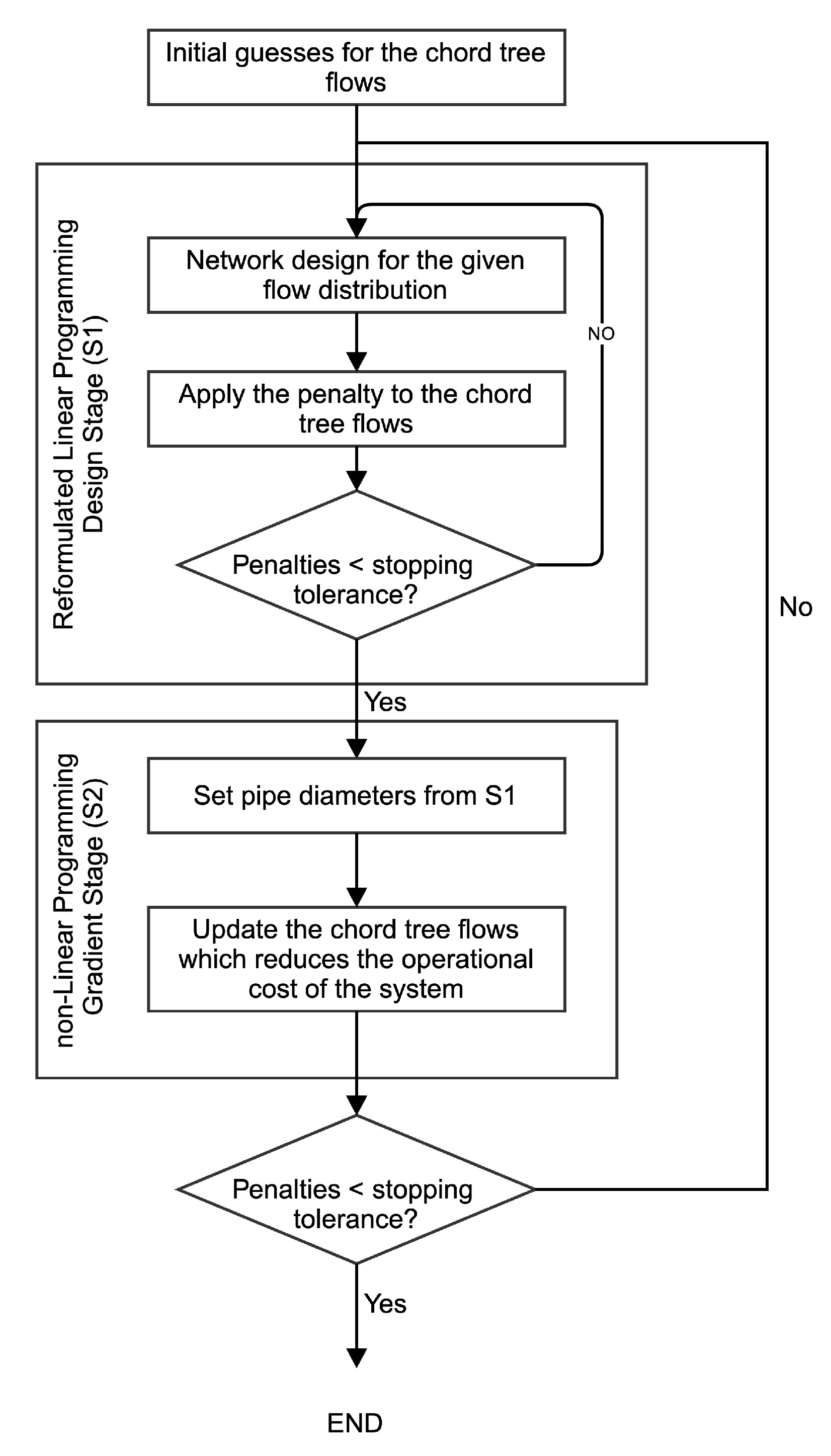
The steps of the proposed methodology are shown in Figure 1. The proposed method decomposes the optimization problem into two stages: (1) an iterative linear programming stage that finds the optimal length for each pipe segment of each pipe, tanks size, pumps capacity, and pump operating point. This stage is performed for given flow distribution in the system for each of the loading conditions; (2) a nonlinear programming stage that finds a new set of flow distributions that reduces the WDS operational cost, tank cost, and pump cost. The following subsections describe both of the above stages.

5.1. Stage 0—The Identification of the Chord Tree and Spanning Tree of a WDS

The graph component that is associated with a WDS can be described as $G=(V,E)$ where V is the set of all nodes of the graph G and E is the set of all pipes of the graph G. For any connected graph G, there must exist at least one subgraph of the graph G that spans G, such a subgraph is called a spanning tree of the graph G. The relative complement of the spanning tree with respect to the graph G is called chord tree. A spanning tree is an acyclic graph which traverses every node in a graph, such that the addition of any chord-tree element creates a loop. A WDS can be partitioned into two subgraphs: a spanning tree $G_{st}=\left(V_{st},E_{st}\right)$, and a co-tree $G_{ct}=\left(V_{ct},E_{ct}\right)$, so that $E_{st}\cup E_{ct}=E$, $E_{st}\cap E_{ct}=\varnothing$. The flows in the spanning tree can be found directly from the co-tree flows. Stage 0 of the proposed methodology is a pre-processing step, in which a spanning tree and chord tree combinations are identified. A spanning tree search algorithm in [31] is used to identify a spanning tree and chord tree combination.

5.2. Stage 1—Iterative LP Design Stage

The first stage of the proposed methodology is to solve the design problem for a given flow distribution. The purpose of this stage is to identify the optimal decision variables for a given flow distribution (i.e., length of the pipe segments for each pipe, maximum and initial storage volume for each tank, maximum pump power for each pump, pump operating power for each pump at each time step). In this stage, the chord tree flows are taken as random initial guesses for the first iteration and as the output from Stage 2 for the subsequent iterations. Then, the flows in the spanning tree pipes can be calculated using Equation (23). By generating flow distribution in this way, the mass balance equation will be always satisfied. The LP model for the first stage of the proposed methodology can be described as:

$$\begin{array}{cc}\mathrm{minimize}\hfill & \left(C{C}_{pipes}+C{C}_{tanks}+C{C}_{pumps}+O{C}_{pumps}+PC\right)\hfill \\ \mathrm{subject}\mathrm{to}\hfill & \mathrm{Constraints}\mathrm{in}\mathrm{Equations}(5)–(11),\left(16\right)–\left(18\right)\mathrm{and}(27)\hfill \end{array}$$

Penalty Reduction

As discussed previously, one drawback of using LPG method is that the set of flow distributions that is parsed to the network design stage of the problem is often infeasible. In the original LPG paper [2], two artificial variables, which behave as valves, are introduced for each loop and quasi-loop to balance the energy equations. These two variables are given a large penalty in the objective function so that the optimization process will try to nullify them if possible.

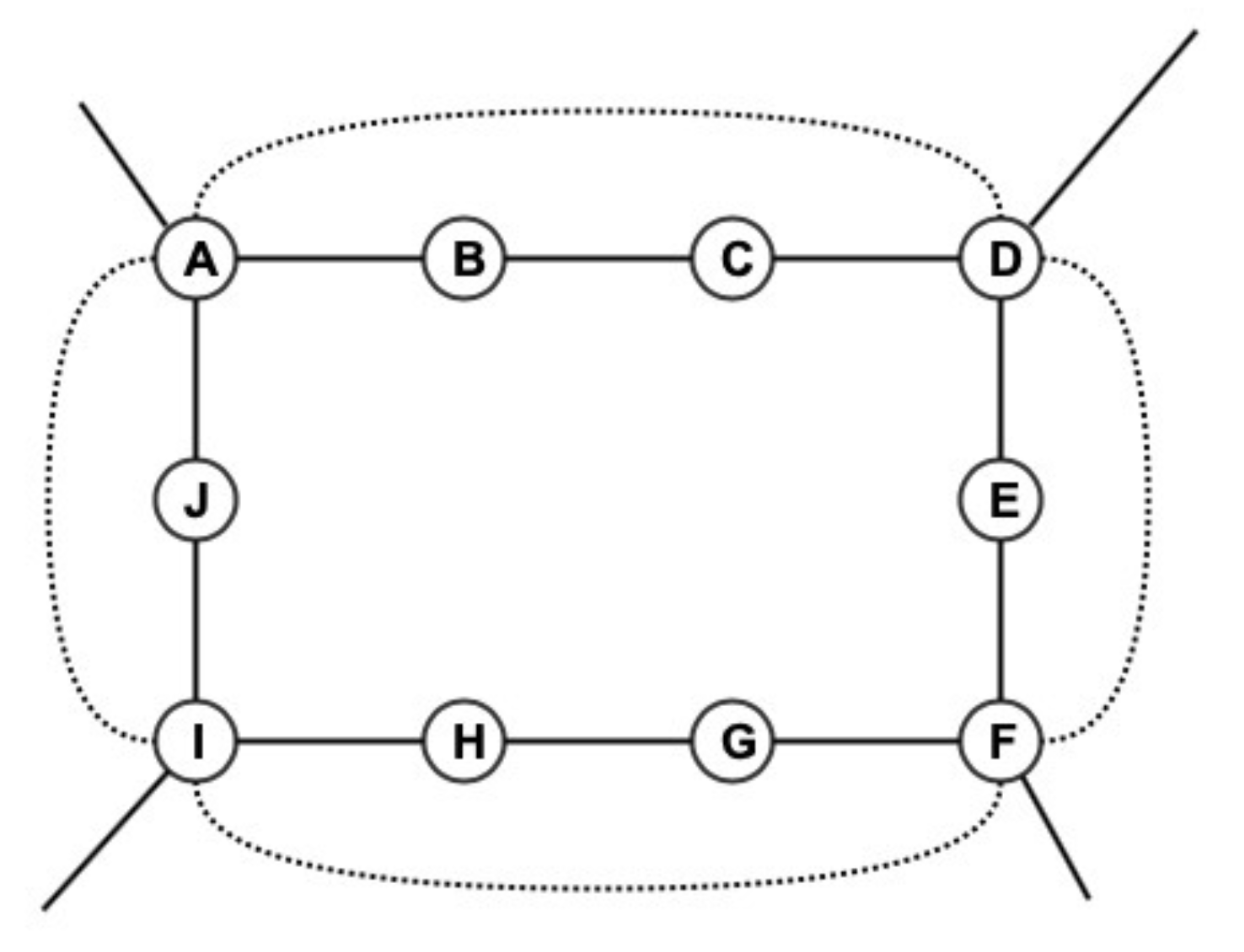
However, the elimination of the penalty is often impossible as the number of loops and the number of loading conditions increases. To demonstrate this, let us consider the 10-link loop shown in Figure 2 which has four superlinks. In this case, if there are more than four loading conditions, the subsystem of the loop energy equations is overdetermined for a given set of flows that represent the loading conditions. This overdetermined subsystem, in most cases, will cause infeasibility in the linear program, which is solved to determine the lengths of the segments in the design problem. This situation will be even exacerbated if there exists shared superlinks between different loops. This is because, in case of a shared link, the degree of freedom in the linear system of equations is reduced by one.

As a result of the above observation, the penalty of the final design in the first (i.e., small two-loop) example of [2] dropped to zero, whereas the final design in the second example (17 loops and 2 loading conditions) has a nonzero penalty of 1.5 billion cost unit which is 250 times the unpenalized network cost (6 million cost units).

In this paper, an iterative method to reduce the penalty cost when designing a network with multiple loading conditions is proposed. The efficient penalty reduction is achieved by using the constraint in Equation (27) to replace the loop and quasi-loops energy equations in the original LPG Equations (13)–(15).

Unlike the LPG method, the constraint in Equation (27) involves the chord flows only. That is, only the flows of chord tree pipes in a WDS network are parsed to the network design stage, as opposed to the LPG in which the flows of all pipes are parsed to the design stage. The flows of the spanning tree pipes are calculated using the chord tree pipe flows using Equation (23). The nodal heads can then be calculated from the spanning tree pipe flows using Equation (24). Moreover, we also modify the objective function to include high penalty cost coefficients for the artificial variables in Equation (26) (${10}^8$ times the typical values of the objective function). Constraint $C_{10}$ at $i-th$ iteration and time t of the inner penalty-reduction iteration becomes:

$${\mathit{R}}_{ct}\left[{\mathit{I}}_{n_{ct}}{\left|{\mathit{q}}_{ct}^{(i,t)}\right|}^{n-1}\right]{\mathit{q}}_{ct}^{(i,t)}-{\mathit{T}}_2{\mathit{h}}^{(i,t)}-{\mathit{a}}_2+{\mathit{a}\mathit{r}\mathit{t}}_1^{(i,t)}-{\mathit{a}\mathit{r}\mathit{t}}_2^{(i,t)}=\mathit{O}$$

(29)

These artificial variables can be directly applied to the chord tree pipe flows at $(i+1)-th$ iteration and time t of the inner penalty-reduction iteration by:

$${\mathit{R}}_{ct}\left[{\mathit{I}}_{n_{ct}}{\left|{\mathit{q}}_{ct}^{(i+1,t)}\right|}^{n-1}\right]{\mathit{q}}_{ct}^{(i+1,t)}={\mathit{R}}_{ct}\left[{\mathit{I}}_{n_{ct}}{\left|{\mathit{q}}_{ct}^{(i,t)}\right|}^{n-1}\right]{\mathit{q}}_{ct}^{(i,t)}+{\mathit{a}\mathit{r}\mathit{t}}_1^{(i,t)}-{\mathit{a}\mathit{r}\mathit{t}}_2^{(i,t)},$$

which can be simplified to:

$${\mathit{q}}_{ct}^{(i+1,t)}={\mathit{q}}_{ct}^{(i,t)}+{\left|{\left({\mathit{R}}_{ct}^{(i,t)}\right)}^{-1}({\mathit{a}\mathit{r}\mathit{t}}_1^{(i,t)}-{\mathit{a}\mathit{r}\mathit{t}}_2^{(i,t)})\right|}^{\left(\right(1/n)-1)}\left({\left({\mathit{R}}_{ct}^{(i,t)}\right)}^{-1}({\mathit{a}\mathit{r}\mathit{t}}_1^{(i,t)}-{\mathit{a}\mathit{r}\mathit{t}}_2^{(i,t)})\right).$$

(30)

The above operation can be used to move the current flow distributions towards the direction of the feasible region. This is because, by updating the chord tree flows using Equation (30), the resulting ${\mathit{q}}_{ct}^{(i+1)}$ and ${\mathit{q}}_{st}^{\left(i\right)}$ must satisfy $C_{1)}$. A new set of spanning tree flows, ${\mathit{q}}_{st}^{(i+1)}$, can be generated based on the ${\mathit{q}}_{ct}^{(i+1)}$ using Equation (23). This spanning tree flows generation process will disperse the values of the two vectors of artificial variables from the chord tree pipes to the spanning tree pipes. Therefore, repeating the Stage 1 using the new chord tree flows, ${\mathit{q}}_{ct}^{(i+1)}$, results in a smaller value of ${\mathit{a}\mathit{r}\mathit{t}}_1^{(i+1)}-{\mathit{a}\mathit{r}\mathit{t}}_2^{(i+1)}$ compared to the value of ${\mathit{a}\mathit{r}\mathit{t}}_1^{\left(i\right)}-{\mathit{a}\mathit{r}\mathit{t}}_2^{\left(i\right)}$. Note that, only one of ${\mathit{a}\mathit{r}\mathit{t}}_1$ and ${\mathit{a}\mathit{r}\mathit{t}}_2$ can have a non-zero value in the optimal solution of the LP solver.

The updated chord tree pipe flows are then used again to generate a set of flow distributions to use in the network design stage, using Equation (23), until the penalties are less than the pre-defined stopping tolerance, after which the network design is parsed to the NLP operational cost optimization stage.

5.3. Stage 2—NLP Descending Stage

The pipe diameters obtained in Stage 1 is now used as the input for Stage 2. The purpose of this stage is to find a new set of flows in the chord tree pipes that reduces the WDS operational cost and the pumps and tanks capital costs. The NLP model for the second stage of the proposed methodology can be described as:

$$\begin{array}{cc}\mathrm{minimize}\hfill & \left(C{C}_{tanks}+C{C}_{pumps}+O{C}_{pumps}\right)\hfill \\ \mathrm{subject}\mathrm{to}\hfill & \mathrm{Constraints}\mathrm{in}\mathrm{Equations}\left(7\right)–\left(12\right),\left(16\right)–\left(18\right)\mathrm{and}\left(27\right)\hfill \end{array}$$

in which, the model decision variables are: (1) flows in the chord tree pipes, (2) the initial and maximum storage volume of each tank, (3) the pump operating power at each time step for each of the pumps in the system, and (4) maximum pump power for each pump.

6. Relation of the Proposed Method to Other LP Methods

The proposed algorithm is an iterative method that optimizes the operation and design of a WDS simultaneously. It consists of two stages: (1) an iterative LP design stage and (2) an NLP stage as shown in Figure 1.

In the first stage of the proposed methodology, the flows in the chord tree pipes are required to be initialized instead of having to initialize for the flows in all pipes, which reduces the number of decision variables by $n_j$ when compared to the existing LPG. In addition, the corresponding spanning tree flows that are calculated from the chord tree flow will satisfy the continuity equations automatically. Moreover, a penalty reduction mechanism is introduced using the new initialization method of the chord tree flows. This is because the penalty cost that is associated with each of the loops and independent paths has to be represented by adding two valves in the original LPG method, whereas the chord tree flows in the proposed method can be corrected within the inner iterations of Stage 1 using Equation (30). As a result, the penalty cost of output from Stage 1 of the proposed methodology will always be minimal.

In the second stage of the proposed methodology, the resistance factors in all pipes are used as the input for this stage and updated chord tree pipe flows are generated by solving NLP problem. This stage is used to replace the search technique used in the LPG method. The LPG method focuses the search of its second stage on the minimization of the pipe and pump capital cost. This can be seen from each of the two case studies in [2] that the initial guesses of the sources’ flow are the same as the optimal sources’ flow (i.e., the sources’ flow and as a result the tanks volumes, remained the same during the iteration process). As a result, LPG method cannot change the amount of water supplied from each of the sources of a WDS, thereby (1) restricting the LPG’s ability to design the tanks in a WDS ($C{C}_{tanks}$) and (2) limiting the LPG’s ability to design and operate the pumps ($C{C}_{pumps}+O{C}_{pumps}$) by fixing the pump flows. Contrarily, the proposed methodology focuses the search of its second stage in the minimization of $C{C}_{tanks}+C{C}_{pumps}+O{C}_{pumps}$ while using the basic design of the network from the result of the first stage.

Comparing the NLP in the second stage of the proposed method with the original NLP formulation shows that the energy balance constraint is a nonlinear function of the flows in the chord tree pipes $q_{ct}$ and flows in the pumps $\widehat{q}$, which has significantly less nonlinearity both in nature and in number compared to the energy balance constraint in original NLP. More specifically the NLP in the second stage is advantageous, because: (1) the number of independent decision variables in flow vector is reduced from the number of pipes to the number of chord tree pipes; (2) the vector of nodal heads is an independent decision variables in NLP formulation whereas it becomes a dependent (and thus it could be eliminated) decision variables in the proposed two-stage formulation; (3) smaller number of constraints is required in the second NLP stage of the proposed two-stage method because of the equality constraint in Equations (13)–(15) are eliminated; (4) because the resistance is a parameter in the second stage NLP, the value of which has been determined in the LP stage, the number of nonlinear terms and the degree of nonlinearity in the second stage NLP of the proposed method offers a lower degree of complexity when compared to the original NLP formulation.

7. Applications

The proposed methodology described in the previous section has been applied to two WDSs, which include a simple network first presented in [21] and a modification of the real-life network first presented in [2]. The Hazen-William formula is used to model the head-loss in both cases studies. The results from nonlinear programming are used as the baseline for comparison to demonstrate the efficacy of the proposed methodology. YALMIP toolbox [32] is used to formulate the optimization problems, lpsolve solver [33] is used to solve the LP problems and ipopt solver [34] is used to solve the NLP problems. The case studies were programmed in Matlab R2018a on an Intel Core i7-7700 running at 3.6 GHz with four cores. The details of both case studies are described in the following subsections. It is important to note that the value for $AD$ and $APPV$ for both case studies are used from [21].

7.1. Case Study 1

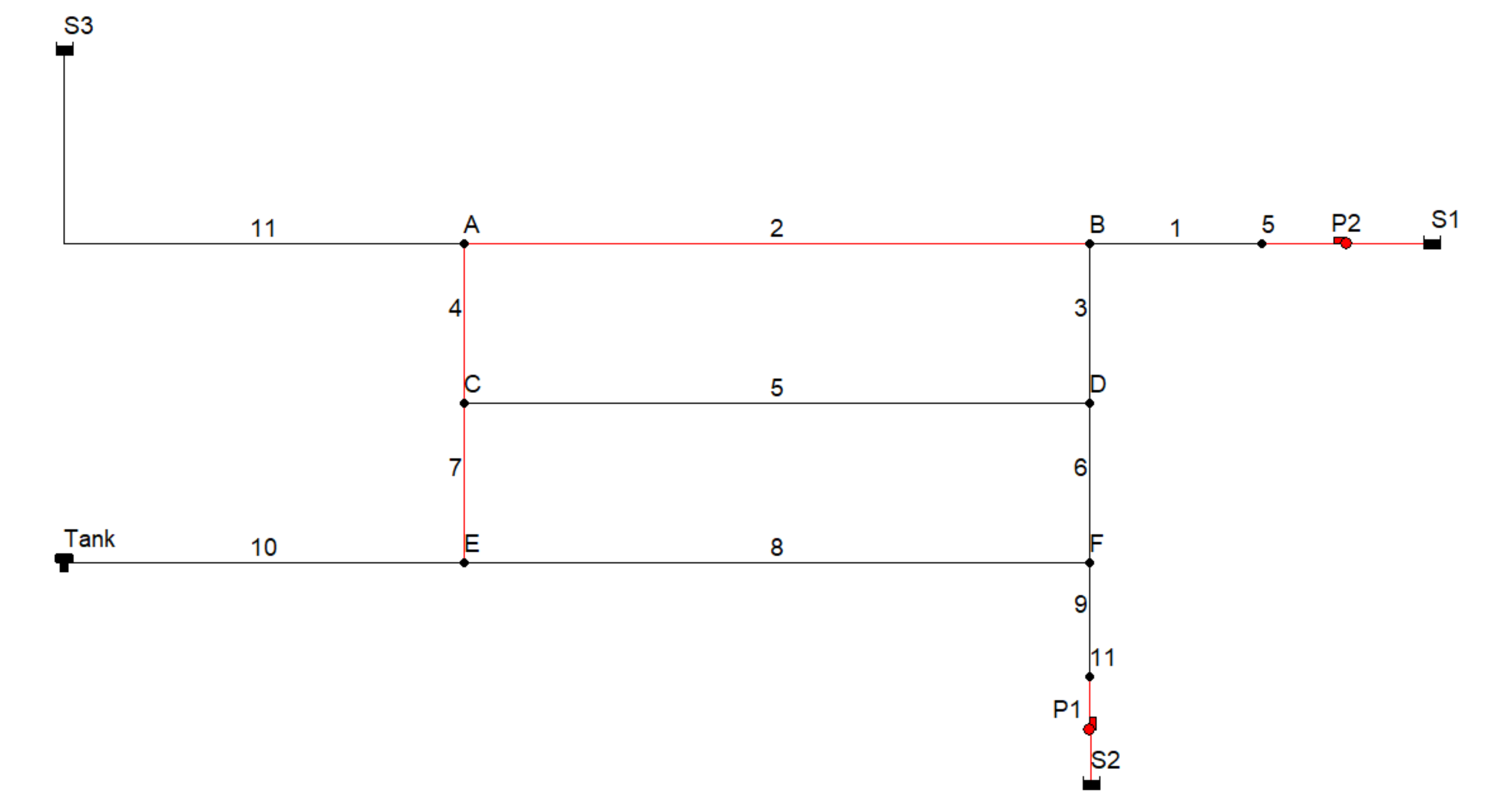
This case study network consists of eight nodes, 11 pipes, three reservoirs, one tank, two pumps, two loops and three independent paths. The layout of this case study network is given in Figure 3. The available pipes’ diameters for both case studies and the corresponding unit costs are shown in

Table 1. Commercially available pipe diameters and unit cost for both case studies.

Pipe Diameter (mm)	Cost ($/m)
25	2
51	5
76	8
102	11
152	16
203	23
254	32
305	50
356	60
406	90
457	130
508	170
559	300
610	550

. The nodes’ data and pipes’ data are summarized in [21] (an EPANET input file can be found in supplementary data). The base run optimization is performed for a typical day starting at 00:00 and ending at 24:00 with four loading condition (i.e., hydraulic time step of six hours). The demand multiplier and electricity tariff for each of the the four loading conditions are shown in second column and fifth column of

Table 2. Demand multipliers and energy tariffs for a typical day divided into four, six, and 12 loading conditions.

Time of Day	Demand Multiplier -			Energy Tariff ($/kWh)
00:00–02:00	-	-	0.2	-	-	0.02
02:00–04:00	-	0.15	0.1	-	0.015	0.01
04:00–06:00	0.2	-	0.3	0.02	-	0.03
06:00–08:00	-	0.7	1.1	-	0.07	0.11
08:00–10:00	-	-	0.9	-	-	0.09
10:00–12:00	0.8	0.65	0.4	0.064	0.065	0.04
12:00–14:00	-	-	0.8	-	-	0.08
14:00–16:00	-	1.0	1.2	-	0.1	0.12
16:00–18:00	1.2	-	1.6	0.12	-	0.16
18:00–20:00	-	1.2	0.8	-	0.12	0.08
20:00–22:00	-	-	0.7	-	-	0.07
22:00–24:00	0.6	0.5	0.3	0.048	0.05	0.03

respectively. The minimum nodal pressure requirement for the unknown head nodes is 30m. The identified spanning tree and chord tree combination is shown in Figure 3. In addition to the base run optimization, the impact of 6 and 12 loading conditions on the solution of the proposed two-stage method and the NLP method have been investigated (data is given in Table 2).

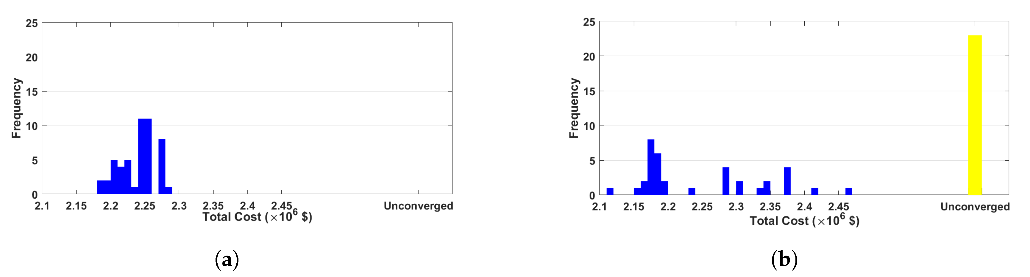
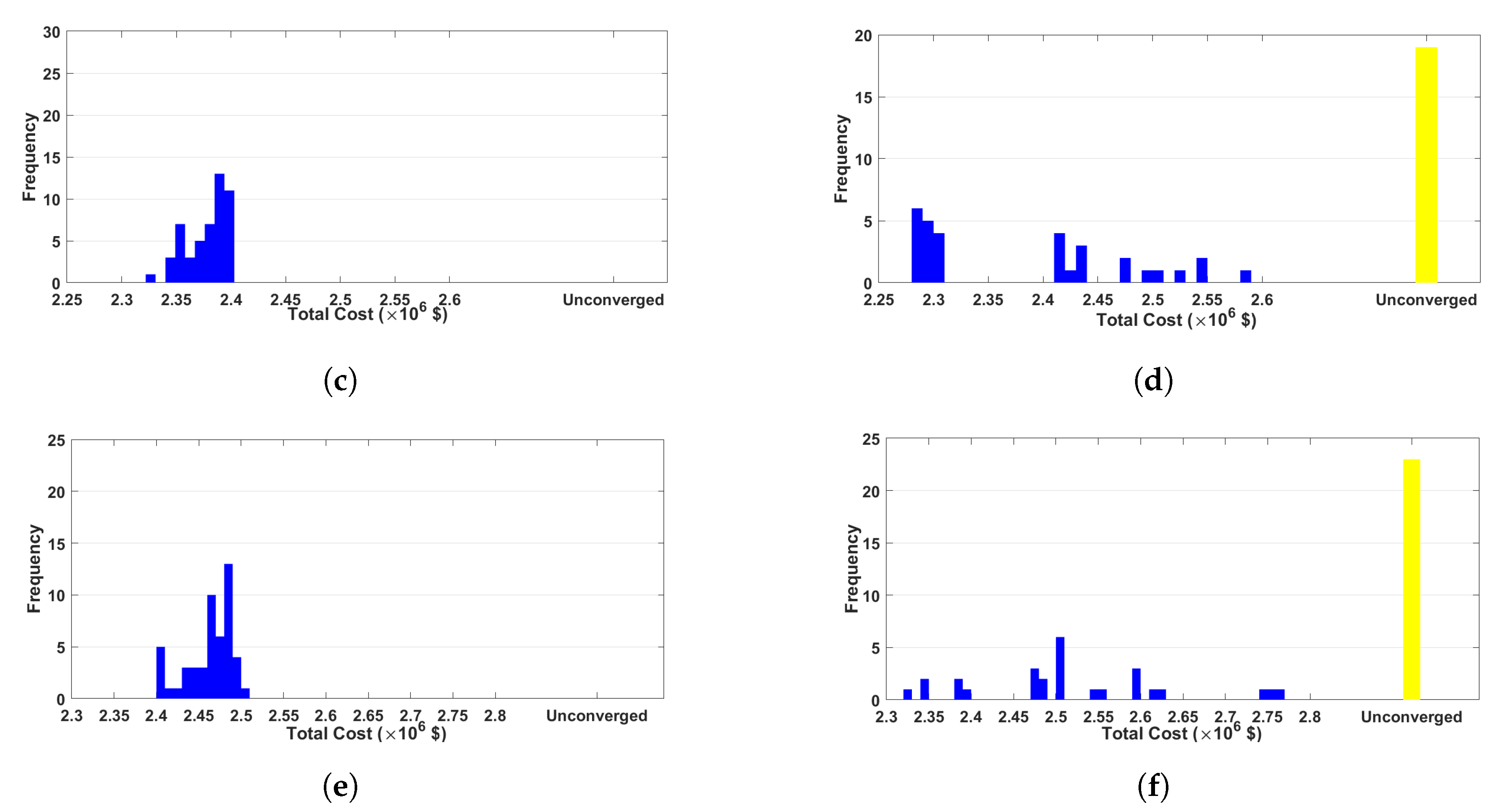
The minimum, maximum, mean and median for all cost components and the total cost of 50 repeated runs with random initial guesses for the chord tree flows were collected. The tolerance value for the inner penalty-reduction iteration (the sum of all artificial variables) is 10 and for the outer cost-reduction iteration is ${10}^{-5}$.

Table 3. Detailed statistics of the cost of each component of the 50 runs with different initial guesses of the flows in the chord tree pipes of the proposed two-stage method and NLP method applied to the two-loop network with four loading conditions (base run). (a) The proposed two-stage method. (b) The original NLP method.

(a)
Statistical Properties ($ × 105)
	Min	Max	Mean (%)	Median	Std. Dev	Std. Err
Pipe Cost	3.52	4.15	3.82 (17%)	3.80	0.19	0.03
Tank Cost	1.26	1.72	1.46 (7%)	1.45	0.10	0.01
Pump Cost	5.18	5.94	5.4 (24%)	5.38	0.19	0.03
Energy Cost	10.85	12.18	11.68 (52%)	11.76	0.36	0.05
Total Cost	21.78	22.91	22.37	22.42	0.28	0.04
(b)
Statistical Properties ($ × 105)
	Min	Max	Mean(%)	Median	Std. Dev	Std. Err
Pipe Cost	2.63	4.43	3.23 (14%)	3.19	0.31	0.05
Tank Cost	0.65	1.40	1.10 (5%)	1.25	0.30	0.05
Pump Cost	5.10	6.72	5.88 (26%)	5.66	0.42	0.07
Energy Cost	11.40	13.39	12.25 (55%)	12.10	0.55	0.09
Total Cost	21.14	24.65	22.46	21.87	0.90	0.15

(a) (Note: 50 runs, all of which are completed with feasible solutions); (b) (Note: 50 runs, 36 of which are completed with feasible solutions).

presents the detailed statistics of the proposed two-stage method (Table 3a) and NLP method (Table 3b) applied to the two-loop network with four loading conditions (base run). Figure 4 presents the histograms for the proposed two-stage formulation and the NLP formulation applied to each of the three loading cases: (1) two-stage method applied to the four, six, and 12 loading conditions in Figure 4a,c,e, respectively and (2) NLP method applied to the four, six, and 12 loading conditions in Figure 4b,d,f, respectively.

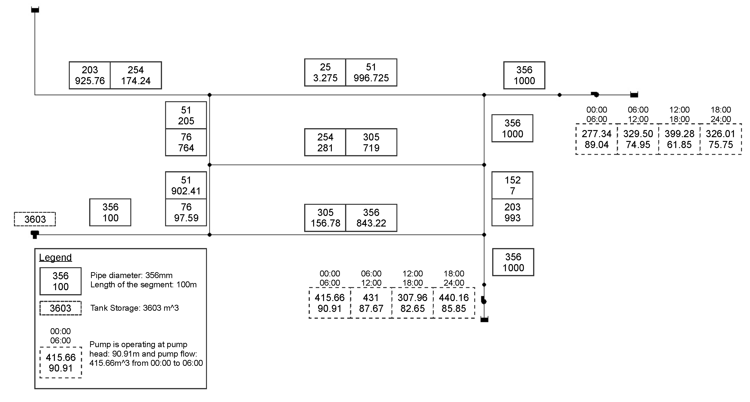
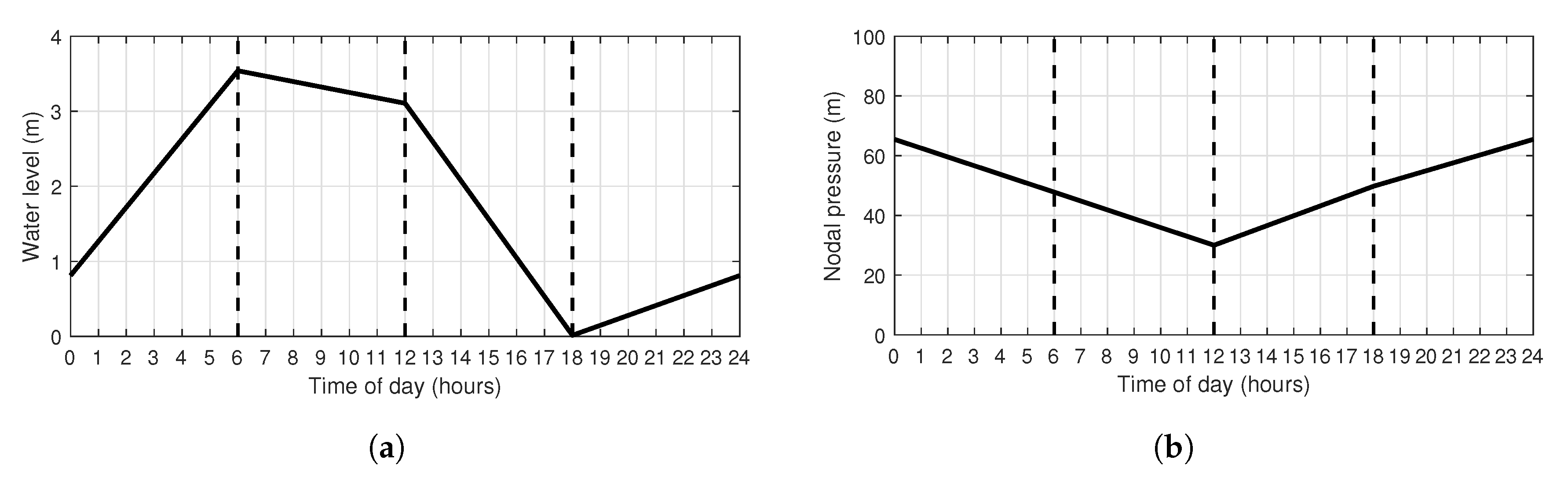
The mean CPU solver time for each of the optimization runs using the proposed two-stage method with the three different loading cases is 1.3, 2.61, 6.29 sec for four, six and 12 loading conditions, respectively. For the original NLP method, the CPU solver time with the three different loading cases is 4.83, 10.04, 17.81 sec for four, six and 12 loading conditions. For the purpose of illustration, the pipe diameters, pump configuration for each of the four loading conditions, and the tank storage of the best base run solution obtained are shown in Figure 5. Figure 6a shows the water level trajectory in the tank over the time of a typical day and Figure 6b shows the pressure profile of the most pressure critical node, Node C, in the system using the network design shown in Figure 5.

As shown in Figure 4a,c,e, the penalty cost in all runs was nullified, indicating that feasible solutions were obtained in all runs when using the two-stage method. This represents a significant improvement when compared to the linear programming stage in the original LPG method. As explained previously, in the LPG, optimizing a WDS with more than one loading condition will often incur penalty costs in the final solution. This penalty costs are handled by the use of dummy valves. These dummy valves, if cannot be eliminated, must be included in the final design as physical valves that should be installed [2]. It is evident from Figure 4 that a smaller minimum cost is obtained by solving the NLP formulation than that by solving the proposed two-stage formulation for the two-loop network (the relative differences between the two-stage method and the NLP method are 3%, 2.5% and 3.5% for the four, six and 12 loading conditions, respectively). However, the mean, standard deviation, and the worst case of the solutions that are found by solving the proposed two-stage formulation are smaller than that are found by solving the NLP formulation (Table 3), which means using the proposed two-stage formulation is able to find a better solution than using the NLP formulation on average and more frequently. In addition, each of the 50 trials performed using the proposed two-stage formulation has successfully yielded a feasible solution for four, six, and 12 loading conditions whereas only 36, 31, and 27 trials out of 50 trails performed using the NLP formulation have successfully found feasible solutions for four, six, and 12 loading conditions respectively. As a result, the proposed two-stage method is more robust in terms of the number of loading conditions when compared to the original NLP method. This robustness will be further fortified in large-scale networks as demonstrated in the next section. In fact, examining large network is the true exam for the developed algorithm since it is expected that NLP methods can handle small problem, but it will be challenged in real-life networks (even mid-size).

Moreover, the optimal solutions obtained using the proposed two-stage method reached an average of $2.237\times {10}^6$ with standard deviation of $0.028\times {10}^6$ and best solution found is $2.178\times {10}^6$ compared to an average of $6.382\times {10}^6$ with standard deviation of $1.21\times {10}^6$ and best solution found is $3.885\times {10}^6$ reported in [21] which used ant colony method. Thus, indicating that the results of the two-stage method outperforms ant-colony in all measures.

7.2. Case Study 2

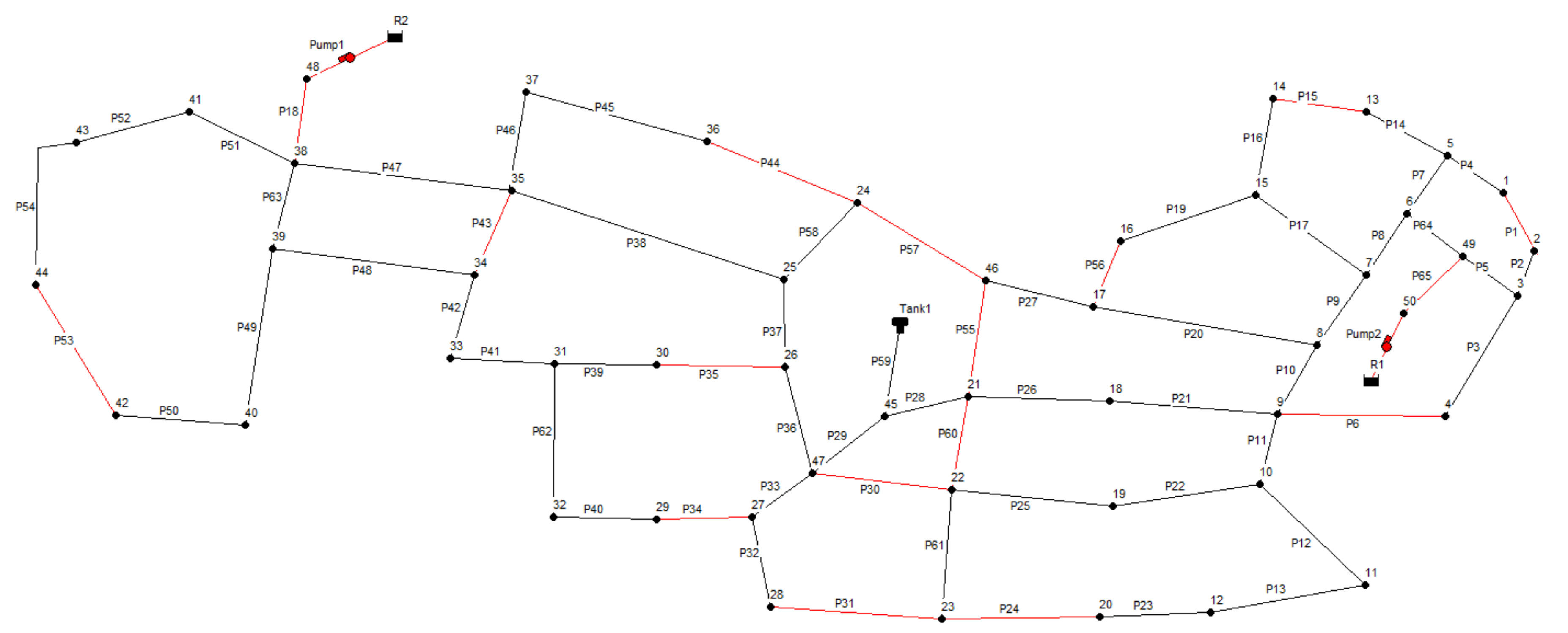
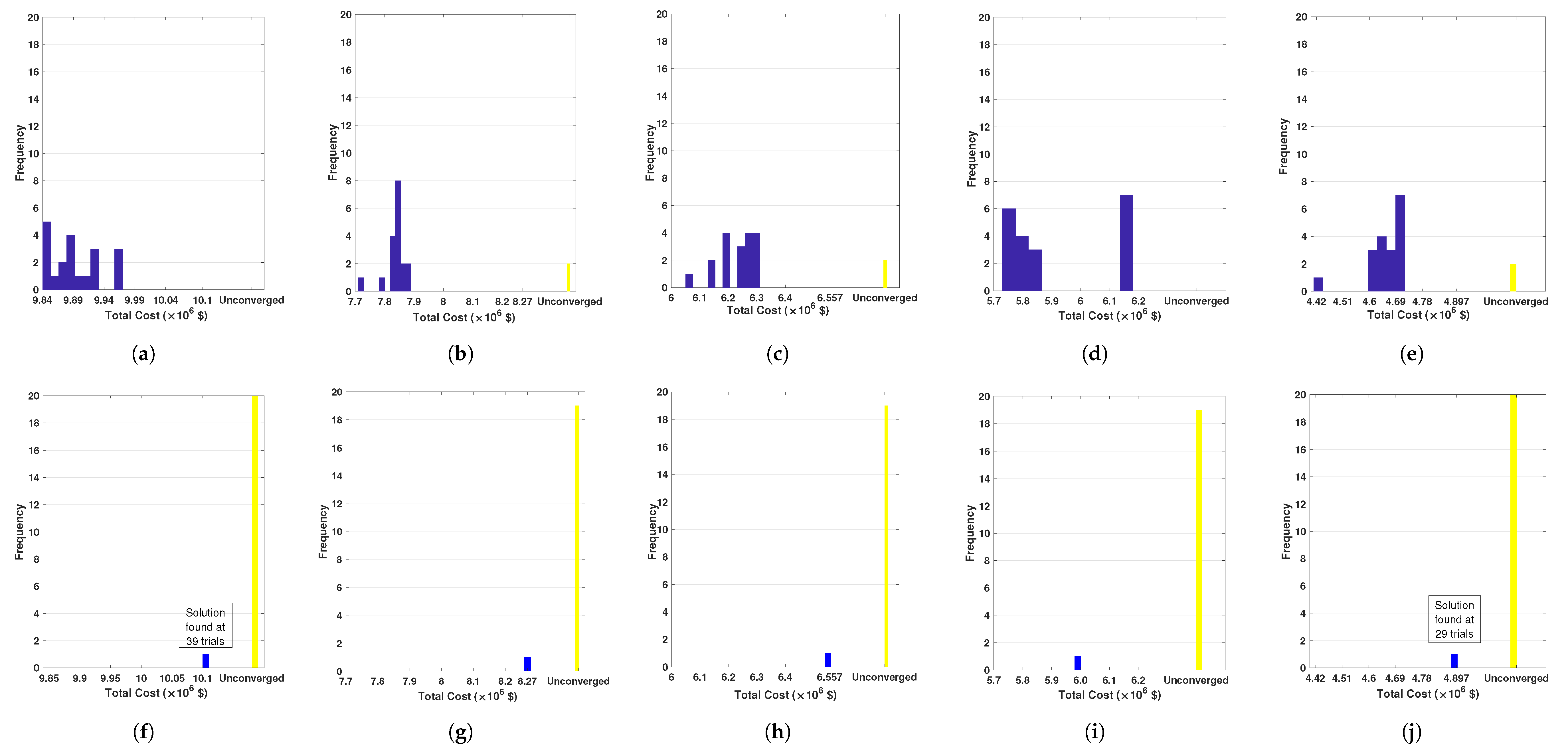
This case study network consists of 50 nodes, 65 pipes, two reservoirs, one tank, two pumps, 14 loops and two independent paths. The layout of this case study network is given in Figure 7. The network used here was derived from [2] with some slight modifications (the reservoir connects to node 45 has been replaced by a tank). This modification introduces a tank into the original system so that the problem can be considered within simultaneous design-operation settings, which is the focus of the paper. The nodes’ data and pipes’ data of this case study network are summarized in [2] (an EPANET input file can be found in supplementary data). The available pipe diameters and their unit cost, demand multiplier and energy tariff for each of the four loading conditions are the same as that of the Case Study 1, which are shown in Table 1 and second and fifth columns in Table 2. The minimum nodal pressure requirement for the unknown head nodes is 30 m. The identified spanning tree and chord tree combination are shown in Figure 7. In addition to the base run optimization, the impact of different reservoir elevation head on the solution of the proposed two-stage method and the NLP method have been investigated. As discussed in the previous section, the second stage of the proposed method focuses on minimizing the total cost using the predetermined pipe configuration from Stage 1. As a result, changing the source node elevations and fixing the demand node elevations can provide additional information on the applicability of the proposed two-stage method. The elevation heads for the reservoirs R1 and R2 are 406 m in the base run optimization, where five additional runs have been performed for different source elevation configurations: (370-320), (320-320), (320-280), (270-240), and (200-200). Note that the first number is the reservoir elevation for R1 and the second number is the reservoir elevation for R2. The total cost of 20 repeated runs with different initial guesses for the chord tree flows were collected. Figure 8 shows the histograms of the proposed two-stage method and NLP method applied to the real-life network with different source elevation configurations. A summary of the best result obtained can be found in the supplementary information.

It is evident from Figure 8 that a smaller minimum cost is obtained by solving the proposed two-stage formulation than that by solving the proposed NLP formulation for the real-life network (the relative differences between the two-stage method and the NLP method are ranging from 2.6% to 6.9%). In addition, all of the 20 trials performed using the proposed two-stage formulation has successfully yielded a feasible solution for two source elevation configurations (200-200) and (320-320). Whereas in the remaining configurations (270-240), (320-280) and (320-320) only two trials out of the 20 trials has failed to converge. In contrast, the NLP method failed to converge in the vast majority of the runs. More specifically, 19 trails out of the 20 trails performed using the NLP method has failed to converge for three source configurations: (270,240), (320,280), and (320,320), whereas none of the 20 trials performed using the NLP formulation has reached a feasible solution for the source elevation configurations (200-200) and (370-320). More trials have been carried out for these two source elevation configurations in order to determine the required number of trails for reaching a feasible solution. In configuration (200,200) a feasible solution has been reached at 39 trails while in configuration (370,320) a feasible solution has been reached at 29 trails. In all configurations, the best result obtained by the two-stage algorithm outperforms the result of the NLP method.

Results from the two case studies demonstrate that the proposed two-stage method (1) can consistently drop the penalty cost in the LP stage, (2) exhibit high robustness when compared to the NLP method that is used as the baseline, (3) produce comparable results for smaller network when compared to the NLP formulation, such as Case Study 1, and produce better solution for a bigger network when compared to the NLP formulation, such as Case Study 2. These advantages are more pronounced as the size and complexity of case study network increase. Furthermore, the solution found by proposed two-stage method ($2.237\times {10}^6\pm 0.04\times {10}^6$) compared favorably with those found in the previous studies. This improvement can be partly attributed to the fact that the proposed two-stage method allows the segmentation of the candidate pipe between two nodes. In addition, the proposed two-stage method is not only more reliable find a feasible solution than meta-heuristics algorithms, but also it does not require any parameter tuning and sensitivity analysis.

8. Conclusions

This paper presents an efficient iterative two-stage LP-NLP method for finding the least-cost operation and design of a water distribution system. In the proposed method, the graph that is associated with a WDS is first decomposed into a spanning tree graph and chord tree graph. Then, a set of initial chord tree pipe flows is used to find a feasible network design. Finally, the feasible network design found in the previous step is used to find a new set of chord tree pipe flows that reduces the WDS operation cost.

The main features of the proposed two-stage LP-NLP method include:

• the iterative LP stage can consistently find a feasible design for a WDS with multiple loading conditions without the need to add additional network elements (such as valves) to the network;
• it exhibits a higher robustness to the increase of the number of loading conditions and the change of the elevations of the reservoir nodes when compared to the NLP formulation and meta-heuristics algorithms (ant colony optimization);
• its performance is not affected by the parameters used so that no parameter tuning is required;
• it is significantly less computational-intensive when compared to evolutionary algorithms, such as genetic algorithm, differential evolution, ant colony optimization, and particle swarm optimization.

It is important to note that the NLP stage of the proposed method uses the network design found in the LP stage of the proposed method. Therefore, the chord tree pipe flows generated by the NLP stage minimize the tank capital cost, pump capital cost, and energy cost subject to the network design found in the LP stage. However, the behavior of the resultant pipe cost that is associated with new chord tree flows is unknown. In addition, this research focused on developing a single objective optimization algorithm, other reliability and resiliency-based objectives could be incorporated in the model by using the epsilon or the weights methods [35] for solving the multi-objective problem as a series of single objective problems. Mechanisms that can be used for solving the multi-objective problem as a series of single objective problems will be an interesting avenue for future research.

References

- Zessler, U.; Shamir, U. Optimal operation of water distribution systems. J. Water Resour. Plan. Manag. 1989, 115, 735–752. [Google Scholar] [CrossRef]
- Alperovits, E.; Shamir, U. Design of optimal water distribution systems. Water Resour. Res. 1977, 13, 885–900. [Google Scholar] [CrossRef]
- Kessler, A.; Shamir, U. Analysis of the linear programming gradient method for optimal design of water supply networks. Water Resour. Res. 1989, 25, 1469–1480. [Google Scholar] [CrossRef]
- Quindry, G.E.; Liebman, J.C.; Brill, E.D. Optimization of looped water distribution systems. J. Environ. Eng. Div. 1981, 107, 665–679. [Google Scholar]
- Shamir, U. Optimal design and operation of water distribution systems. Water Resour. Res. 1974, 10, 27–36. [Google Scholar] [CrossRef]
- Murphy, L.; Simpson, A.; Dandy, G. Pipe Network Optimization Using an Improved Genetic Algorithm; Department of Civil and Environmental Engineering, University of Adelaide: Adelaide, Australia, 1993. [Google Scholar]
- Simpson, A.; Dandy, G.; Murphy, L. Genetic algorithms compared to other techniques for pipe optimization. J. Water Resour. Plan. Manag. 1994, 120, 423–443. [Google Scholar] [CrossRef] [Green Version]
- Dandy, G.; Simpson, A.; Murphy, L. An improved genetic algorithm for pipe network optimization. Water Resour. Res. 1996, 32, 449–458. [Google Scholar] [CrossRef] [Green Version]
- Savic, D.; Walters, G. Genetic algorithms for least-cost design of water distribution networks. J. Water Resour. Plan. Manag. 1997, 123, 67–77. [Google Scholar] [CrossRef]
- Loganathan, G.; Greene, J.; Ahn, T. Design heuristic for globally minimum cost water-distribution systems. J. Water Resour. Plan. Manag. 1995, 121, 182–192. [Google Scholar] [CrossRef]
- Cunha, M.; Sousa, J. Water distribution network design optimization: Simulated annealing approach. J. Water Resour. Plan. Manag. 1999, 125, 215–221. [Google Scholar] [CrossRef]
- Lippai, I.; Heaney, J.; Laguna, M. Robust water system design with commercial intelligent search optimizers. J. Comput. Civ. Eng. 1999, 13, 135–143. [Google Scholar] [CrossRef]
- Geem, Z.; Kim, J.; Loganathan, G. Harmony search optimization: Application to pipe network design. Int. J. Model. Simul. 2002, 22, 125–133. [Google Scholar] [CrossRef]
- Geem, Z. Optimal cost design of water distribution networks using harmony search. Eng. Optim. 2006, 38, 259–277. [Google Scholar] [CrossRef]
- Eusuff, M.; Lansey, K. Optimization of water distribution network design using the shuffled frog leaping algorithm. J. Water Resour. Plan. Manag. 2003, 129, 210–225. [Google Scholar] [CrossRef]
- Suribabu, C.; Neelakantan, T. Design of water distribution networks using particle swarm optimization. Urban Water J. 2006, 3, 111–120. [Google Scholar] [CrossRef]
- Montalvo, I.; Izquierdo, J.; Pérez, R.; Tung, M. Particle swarm optimization applied to the design of water supply systems. Comput. Math. Appl. 2008, 56, 769–776. [Google Scholar] [CrossRef] [Green Version]
- Maier, H.; Simpson, A.; Zecchin, A.; Foong, W.; Phang, K.; Seah, H.; Tan, C. Ant colony optimization for design of water distribution systems. J. Water Resour. Plan. Manag. 2003, 129, 200–209. [Google Scholar] [CrossRef] [Green Version]
- Zecchin, A.; Simpson, A.; Maier, H.; Leonard, M.; Roberts, A.; Berrisford, M. Application of two ant colony optimisation algorithms to water distribution system optimisation. Math. Comput. Model. 2006, 44, 451–468. [Google Scholar] [CrossRef] [Green Version]
- Zecchin, A.; Maier, H.; Simpson, A.; Leonard, M.; Nixon, J. Ant colony optimization applied to water distribution system design: Comparative study of five algorithms. J. Water Resour. Plan. Manag. 2007, 133, 87–92. [Google Scholar] [CrossRef] [Green Version]
- Ostfeld, A.; Tubaltzev, A. Ant colony optimization for least-cost design and operation of pumping water distribution systems. J. Water Resour. Plan. Manag. 2008, 134, 107–118. [Google Scholar] [CrossRef]
- Baños, R.; Gil, C.; Agulleiro, J.; Reca, J. A memetic algorithm for water distribution network design. In Soft Computing in Industrial Applications; Springer: Berlin/Heidelberg, Germany, 2007; pp. 279–289. [Google Scholar]
- Suribabu, C. Differential evolution algorithm for optimal design of water distribution networks. J. Hydroinformatics 2010, 12, 66–82. [Google Scholar] [CrossRef]
- Vasan, A.; Simonovic, S. Optimization of water distribution network design using differential evolution. J. Water Resour. Plan. Manag. 2010, 136, 279–287. [Google Scholar] [CrossRef]
- Zheng, F.; Zecchin, A.; Simpson, A. Self-adaptive differential evolution algorithm applied to water distribution system optimization. J. Comput. Civ. Eng. 2012, 27, 148–158. [Google Scholar] [CrossRef] [Green Version]
- Mala-Jetmarova, H.; Sultanova, N.; Savic, D. Lost in optimisation of water distribution systems? A literature review of system operation. Environ. Model. Softw. 2017, 93, 209–254. [Google Scholar] [CrossRef] [Green Version]
- Krapivka, A.; Ostfeld, A. Coupled genetic algorithm—Linear programming scheme for least-cost pipe sizing of water-distribution systems. J. Water Resour. Plan. Manag. 2009, 135, 298–302. [Google Scholar] [CrossRef]
- Zheng, F.; Simpson, A.R.; Zecchin, A.C. A combined NLP-differential evolution algorithm approach for the optimization of looped water distribution systems. Water Resour. Res. 2011, 47. [Google Scholar] [CrossRef] [Green Version]
- Elhay, S.; Simpson, A.R.; Deuerlein, J.; Alexander, B.; Schilders, W.H. Reformulated co-tree flows method competitive with the global gradient algorithm for solving water distribution system equations. J. Water Resour. Plan. Manag. 2014, 140, 04014040. [Google Scholar] [CrossRef] [Green Version]
- Schilders, W. Solution of indefinite linear systems using an LQ decomposition for the linear constraints. Linear Algebra Its Appl. 2009, 431, 381–395. [Google Scholar] [CrossRef] [Green Version]
- Qiu, M.; Alexander, B.; Simpson, A.; Elhay, S. WDSLib: A Water Distribution System Simulation Test Bed. Environ. Model. Softw. submitted.
- Löfberg, J. YALMIP: A toolbox for modeling and optimization in MATLAB. In Proceedings of the CACSD Conference, Taipei, Taiwan, 2–4 September 2004; Volume 3. [Google Scholar]
- Berkelaar, M.; Eikland, K.; Notebaert, P. Lpsolve: Open Source (Mixed-Integer) Linear Programming System; Eindhoven University of Technology: Eindhoven, The Netherlands, 2004; Volume 63. [Google Scholar]
- Wächter, A.; Biegler, L.T. On the implementation of an interior-point filter line-search algorithm for large-scale nonlinear programming. Math. Program. 2006, 106, 25–57. [Google Scholar] [CrossRef]
- Cohon, J.L. Multiobjective Programming and Planning; Courier Corporation: Chelmsford, MA, USA, 2004; Volume 140. [Google Scholar]
Figure 1.
Flowchart of the proposed methodology.
Figure 2.
A small example of the superlinks for the pipes in a looped WDS (dotted lines are superlinks).
Figure 3.
Layout of a two-loop network (the chord tree pipes are highlighted in red).
Figure 4.
Histogram of the total cost after applying the proposed two-stage formulation and the NLP formulation to the two-loop network with different number of loading cases (50 runs for each of the loading cases). (a) Two-stage method applied to case study 1 with 4 loading conditions; (b) NLP method applied to case study 1 with 4 loading condition; (c) Two-stage method applied to case study 1 with 6 loading condition; (d) NLP method applied to case study 1 with 6 loading condition; (e) Two-stage method applied to case study 1 with 12 loading condition; (f) NLP method applied to case study 1 with 12 loading condition.
Figure 5.
The detailed solution of the two-loop network with four loading conditions using the proposed two-stage LP-NLP method.
Figure 6.
The tank levels and pressure profile of the base run solution obtained for the two-loop network. (a) The change of tank water level over time of a typical day of the best solution obtained for the two-loop network; (b) The change of pressure in the pressure critical node over time of a typical day of the best solution obtained for the two-loop network.
Figure 7.
Layout of a real-life network (the chord tree pipes are highlighted in red).
Figure 8.
Histogram of the total cost after applying the proposed two-stage formulation and the NLP formulation to the real-life WDS with different reservoir elevations (20 runs for each of the reservoir configurations). (a) Two-stage method applied to case study 2 with reservoir configuration (200-200); (b) Two-stage method applied to case study 2 with reservoir configuration (270-240); (c) Two-stage method applied to case study 2 with reservoir configuration (320-280); (d) Two-stage method applied to case study 2 with reservoir configuration (320-320); (e) Two-stage method applied to case study 2 with reservoir configuration (370-320); (f) NLP method applied to case study 2 with reservoir configuration (200-200); (g) NLP method applied to case study 2 with reservoir configuration (270-240); (h) NLP method applied to case study 2 with reservoir configuration (320-280); (i) NLP method applied to case study 2 with reservoir configuration (320-320); (j) NLP method applied to case study 2 with reservoir configuration (370-320).