Assessing Groundwater Vulnerability: DRASTIC and DRASTIC-Like Methods: A Review


Department of Mathematics and Computer Science, Ovidius University of Constanta, 900527 Constanta, Romania
Water 2020, 12(5), 1356; https://doi.org/10.3390/w12051356
Submission received: 30 March 2020
/
Revised: 7 May 2020
/
Accepted: 8 May 2020
/
Published: 11 May 2020
(This article belongs to the Special Issue Assessing Water Quality by Statistical Methods)
Abstract
:Groundwater vulnerability studies are sources of essential information for the management of water resources, aiming at the water quality preservation. Different methodologies for estimating the groundwater vulnerability, in general, or of the karst aquifer, in particular, are known. Among them, DRASTIC is one of the most popular due to its performance and easy-to-use applicability. In this article, we review DRASTIC and some DRASTIC-like methods introduced by different scientists, emphasizing their applications, advantages, and drawbacks.
1. Introduction
In recent decades, water scarcity and its pollution became a major issue all over the world. Preserving the groundwater quality is very important for assuring the drinking water resources, given that billions of people all over the world do not have access to water or suffer from water scarcity [1].
Since 1968, when Margat [2] introduced the concept of groundwater vulnerability, many definitions were proposed for this concept. For example, Hirata and Bertolo [3] defined the groundwater vulnerability as “the property of a groundwater system that depends on the sensitivity of the material in permitting the degradation of the saturated zone by pollutant substances originating from human activities”, while the National Research Council [4] defined this term as “the relative ease with which a contaminant (in this case a pesticide) applied on or near the land surface can migrate to the aquifer of interest under a given set of agronomic management practices, pesticide characteristics, and hydrogeological sensitivity conditions”.
The intrinsic vulnerability describes the water vulnerability to different pollutants (independent of their nature) resulted from human activities and is related to the hydrological, geological, and hydrogeological aquifer’s characteristics. Given that the aquifers have different reactions to the same contaminant due to their physicochemical characteristics, the specific vulnerability shows the groundwater vulnerability to a pollutant (or a group of pollutants), determined by the pollutant’s properties, taking into account the time of impact, its intensity, and the interaction between the intrinsic vulnerability components and the contaminant [5,6].
Adams and Foster [7] emphasized that the aquifer vulnerability depends on the properties of the layers situated above the saturated zone to attenuate the pollutants’ effect, by retention or neutralization by chemical reactions.
Gogu and Dassargues [6] divided the approaches of assessing the groundwater vulnerability in three groups, as a function of the groundwater protection. The first group takes into account only the soil and unsaturated zone, the second one takes into consideration the groundwater flow and the contaminant transfer to some extent [8], whereas the third focuses on the soil, the unsaturated medium, and the aquifer.
Different approaches are used for estimating groundwater vulnerability. They can be grouped into three categories. The first group is formed by the index-based methods, which take into consideration only the characteristics of soil and unsaturated zone. They are divided into Hydrogeological Complex and Settings methods (HCS) [9]; Matrix Systems [10], approaches based on the combination of two parameters, and Rating Systems [11,12,13]. They work by building water vulnerability groups using different ratings associated with the physical characteristics of the study media. The second group contains the statistical approaches that assess the groundwater vulnerability through statistical analysis or regression models [14,15,16]. The third one contains the methods based on simulation, which uses simulation techniques for forecasting the processes related to contaminant transport [17,18,19,20]. The index-based techniques have the advantage that they do not depend on data availability or similarities [21].
The procedures that belong to the first and second categories are used for studying the intrinsic vulnerability of large areas [22].
The most used index methods for studying the groundwater vulnerability are DRASTIC [23], GOD [12], AVI rating system [13], DIVERSITY [24], ISIS [11], PRAST [25], SEEPAGE, SINTACS [26,27,28,29]. For the karst aquifer, EPIK [5], REKS [30], RISKE [31], RISKE 2 [32], COP and COP + K [33,34], PaPRIKa [35], PI and the Slovene approach [36,37] have been proposed.
Introduced in 1985, DRASTIC is among the most popular approaches used in groundwater vulnerability estimation due to its capability and easy-to-use. In the following, we shall focus on reviewing this method, and some of the DRASTIC-like procedures that aim to improve the performance of the groundwater vulnerability estimation, emphasizing the differences between them. We shall not focus on the methods assessing the groundwater vulnerability for the karst aquifer because of the extensive literature for the general case and the lack of space.
Some classifications of the methods that will be presented in next sections are:
- Based on the extent of their use:
- With general applicability—DRASTIC, GOD
- For specific regions—SINTACS, DRAMIC, DRIST, DRAV
- That considers the land use—DRASTIC-LU, DRASIC-LU, SINTACS-LU
- For urban area—DRAMIC, DRASTICA
- Based on the specific vulnerabilities assessed:
We shall indicate the references to the articles treating these methods in the next sections, together with a description of approaches.
The methods (and corresponding parameters) for groundwater vulnerability assessment discussed in this article are summarized in Table 1.
2. DRASTIC
DRASTIC is a model that considers the main hydrological and geological factors with a potential impact on aquifer pollution. Its acronym stands for D—depth to groundwater, R—recharge rate, A—aquifer, S—soil, T—topography, I—vadose zone’s impact, and C—aquifer’s hydraulic conductivity [38].
The depth to water table (D) [m] is the thickness of the layer crossed by the pollutant before reaching the aquifer. The aquifer vulnerability is inverse proportional to the depth to the water table.
The net recharge (R) [mm/year] represents the volume of infiltrated water that reaches the aquifer. The contamination possibility increases if the net recharge increases. Three types of recharges can be distinguished: direct, indirect, and localized [39,40].
The aquifer media (A) consists of different types of rocks serving as an aquifer.
The upper part of the vadose zone, with intense biological activity, is defined to be the soil media (S).
The topography (T) (%) is defined by the terrain slope, together with its variation. A low slope will determine a small surface flow and a high pollution risk.
The vadose zone’s impact (I)—The unsaturated or discontinuously saturated layer situated above the water table is called vadose. The pollutant’s transfer is influenced by the vadose zone’s lithology.
The aquifer hydraulic conductivity (C) is the aquifer materials’ capacity to leave the water to pass through it. The aquifer vulnerability is low for reduced hydraulic conductivities.
The hypotheses of the DRASTIC models are:
- The pollutants are produced at the surface of the Earth;
- The pollutants are transported into the soil by precipitation;
- The pollutants’ travel velocity is that of the water;
- The affected area must be big enough.
Firstly, a rate from 1 to 10 is assigned to each parameter, 1 being the least important [38]. Then, the DRASTIC index score is built, using the weights fixed for each parameter. The formula for DRASTIC index is:
where R is the rate and w is the parameter weight.
DRASTIC index = DRDw + RRRw + ARAw + SRSw + TRTw + IRIw + CRCw
The weights have been set up by EPA (the United States Environmental Protection Agency) based on the experts’ knowledge after studying different regions. In the original DRASTIC algorithm the weights range from 1 to 5 (1 being the least important), the smallest possible index score is 23 and the highest, 230. Table 2 and Table 3 contain the weights and ratings of the components, firstly provided in [38]. Lower groundwater vulnerability is described by a lower index score.
Different authors [41,42] pointed out the DRASTIC results’ accuracy, the small amount of input data, its application’s low cost [38,43], reduced computational time, and simple computational procedure [44]. DRASTIC proved to be useful for evaluating the aquifer vulnerability in priority monitoring areas and as a valuable indicator where detailed hydrogeological evaluation is necessary. Other authors emphasized the limited validation procedure of the DRASTIC methodology [45,46] and a low correlation between the experimental data and the model’s output [47,48]. Wang et al. [49] remarked on the necessity of procedure adaption for urban areas, while the parameters’ weight choice in the DRASTIC index was criticized by Merchant [50]. Therefore, several approaches were proposed for improving the groundwater vulnerability estimation accuracy, each of them involving a different number of parameters. In the following, we shall present some of these methods and the rationale for their use.
Although the DRASTIC model was intended to be used in mapping applications, it was not expressly designed for use in a GIS, its initial applications employing a manual map overlay and computation procedure [50]. The main importance of vulnerability maps is that their analysis can provide effective information for making informed decisions for water management [51].
Merchant et al. [52] were the first that used GIS for DRASTIC implementation. Since then, due to their capability of retrieving, storing, organizing, analyzing, and presenting geographically referenced spatial data, GIS methods have been successfully employed for assessing the groundwater vulnerability [53,54,55,56,57,58,59,60].
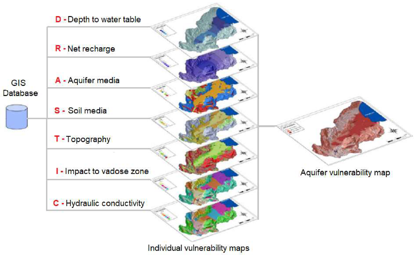
The main GIS advantage is its efficiency of combining data layers and changing the parameters used for the vulnerability classification [49]. For producing a groundwater pollution risk map (Figure 1), it is necessary to prepare the seven individual maps (one for each component in the model). Therefore, all data should be available, accurate enough [50], and introduced in a GIS database.
The D parameter layer is generated using topographic maps. Then, the IDW method is applied for interpolating the water level data and obtaining the depth to the water layer. The general water balance equations are used for generating the recharge layer, R. The lithology, and the type of aquifer media are considered for the estimation of the A factor. The soil media, S, is determined by using the soil textural classification chart. The topographic slope, T, is determined by using a digital elevation model and the data extraction from the topography layer. Then the slope layer (%) is generated, and the range is reclassified taking into account the DRASTIC ranges. The impact of the V factor is determined using the depth to the water layer and the well logs report. The hydraulic conductivity data is retrieved by experimental measurements. Finally, the pollution risk layer is produced using the seven layers previously built by GIS, and all the DRASTIC thematic layers are combined [62].
3. Modified DRASTIC (DRASTICM)
Scientific studies pointed out that geologic structures have a significant impact on highly fractured environments’ vulnerability. Therefore, in a study performed for a region form Nicaragua, Mendoza and Barmen [63] modified the DRASTIC index by including the influence of the length, connectivity, and lineament density. They introduced the lineament influence, denoted by M, in the new model, called Modified DRASTIC, whose index, MDI, is defined by
where R is the rating, M is the lineament factor.
A rate between 0 and 3 was assigned to the influence of the lineament.
Data collected from the field and photographic interpretation were normalized and combined in a map to assess the lineament influence. This map and the other seven (from DRASTIC) contributed to building the Modified DRASTIC map.
Mendoza and Barmen [63] also proposed the classification of groundwater vulnerability degree as very high (MDI > 199), high (MDI between 160 and 199), moderate (MDI in the range 120–159), low (MDI between 80 and 119), and very low (MDI < 79).
The results show that D and T are the factors with a significant influence on vulnerability prediction. Compared with DRASTIC, the modified DRASTIC gave a better estimation of the contamination risk in zones with high fractured structures.
4. DRIST and Modified DRASTIC
Introduced for investigating the underground water vulnerability in Grombalia, the DRIST model was adapted to the hydrogeological system properties from this region. DRIST considers only parameters related to the unsaturated aquifer zone, while DRASTIC works with the aquifer saturated zone characteristics [40]. The calculation of the DRIST vulnerability index is similar to that for DRASTIC (but ignoring A and C parameters).
In the same article, Chenini et al. [40] proposed a Modified DRASTIC method. The difference between these approaches resides in the estimation of the factors A and I. In the new one the lithology is substituted by the permeability, as suggested in [64]. The other maps are created by the same procedure as in DRASTIC.
The permeability map of the vertical vadose zone is realized based on the vertical permeability formula:
where K1 is the vertical average permeability (m/s), H—the unsaturated zone total thickness (m), hi—the thickness of the ith layer (m), ki—the permeability of the ith layer (m/s), and p—the number of layers [64].
The saturated zone’s permeability map is determined using the formula of the horizontal permeability [65]:
where K2 is the average horizontal permeability (m/s), hi, ki and p have the same significance as in formula (3), while at the denominator of formula (10) is the saturated zone total thickness (m).
Comparing the two vulnerability maps, Chenini et al. [40] showed that there are differences between them. The area with medium vulnerability is more significant in the Modified DRASTIC due to the minimization of the saturated zone effect, as an effect of the permeability replacement by lithology in the process of parameters’ estimation. DRIST map reflects the effect of removing the factors related to the saturated zone.
Sakala et al. [66] used the same model and a neural network approach to generate a groundwater vulnerability model. The network used as input the DRIST parameters, and as the training dataset, the sulfate and Total Dissolved Solids (TDS) concentrations retrieved from five groundwater samples. The groundwater vulnerability model was finally obtained by applying a fuzzy operator for combining the training and classification results. The model’s results are well correlated with the available data and the output of the DRIST model.
5. DRAV
DRAV is a model designed by modifying DRASTIC for taking into account the groundwater characteristics from the arid zones [67]. Since generally, in those areas, there is no horizontal runoff, the DRASTIC T term was removed, and S was replaced by V (vadose zone’s lithology). The factors D, R, and A were kept in the new model.
The DRAV index is a linear combination of the factors D, R, A, and V with the normalized weights 0.20, 0.15, 0.31, and 0.34, respectively.
The scores for the D factor are 1, 2, 3, 5, 7, 10, for groundwater depths (m) greater than 30, in the interval (10, 30], between 6 and 10, in the interval (3, 6], in the range 1–3, less than 1, respectively [66].
The scores for the R factor are 1, 2, 4, 6, 8, 10, for recharge modules (×104 m3/km2/area) less than 5, in the interval [5, 10), between 10 and 20, from 20 to 30, in the interval [30, 50), greater than 50, respectively [67].
The scores for the A factor are 1, 3, 5, 7, and 10, for a storativity (m3/day/m) smaller than 2, between 2 and 20, in the interval [20, 200), from 200 to 1000, and greater than 1000, respectively [66].
The scores (for the V factor) 10, 4, 2, and 1 were associated with Sandy gravel, Sandy loam, Sandy clay, and Silty and fine sand, respectively [67].
Five classes of phreatic water vulnerability (extremely high, high, medium, low, and extremely low) corresponds to vulnerability indices above 8, the interval (6, 8], between 4 and 6, the interval (2, 4], , respectively.
DRAV was used to analyze the pore groundwater in the northwestern part of China, but no comparison with other methods is provided. Therefore more studies are necessary to validate this approach.
6. DRAMIC
Many scientists emphasized the limitations of DRASTIC’s application for urban areas [49,68], as follows. (1) The terrain where the cities are situated is mostly flat, so the T factor in the DRASTIC model is not relevant. (2) The values of the soil media can be hardly obtained because the ground surface is mostly covered by concrete. (3) The hydraulic conductivity is not relevant. Therefore, they built the DRAMIC index, by replacing in DRASTIC the S factor by the thickness of the aquifer (M), and the C factor by the contaminant impact (denoted by C as well). It must be noticed that DRAMIC does not consider the pollutants’ properties, but its stability and infiltration capacity into the aquifer. The parameters (and ratings) in DRAMIC are [49]:
- Aquifer thickness (m): 0–6 (9), 6–15 (7), 15–25 (5), 25–32 (4), 32–40 (3), 40–50 (2), >50 (1);
- Contaminant’s characteristics:
- ▪
- Stability, infiltration easiness (9)
- ▪
- Stability, infiltration relative easiness (7)
- ▪
- Stability, infiltration uneasiness, and Relative stability, infiltration easiness (5)
- ▪
- Relative stability, infiltration relative easiness (4)
- ▪
- Relative stability, infiltration uneasiness, and Instability, infiltration easiness (3)
- ▪
- Instability, infiltration relative easiness (2)
- ▪
- Instability, infiltration uneasiness (1)
The DRAMIC Index is computed by the relation
where R is the rating.
DRAMIC index = 2DR + 3RR + 4AR + 2MR + 5IR + 1CR
The main factors considered in DRAMIC are the stability of the pollutant and the easiness of the pollutant infiltration. The results of this model applied in a study from China (Wuhan region) were compared with the field data, showing a good correlation. Despite promising results, other studies are needed to validate this method for other urban areas.
7. DRASTICA
DRASTICA is a modified DRASTIC model, which includes the anthropogenic influence in urbanized environments [68,69]. A new factor (A-anthropic factor) was introduced, with the weight equal to 5. The index is computed as in DRASTIC, adding the new term, ARAw, where AR is the rating and Aw the weight. The anthropic factors and the rating assigned are the following [68]: Effluents/sewage/industrial waste (untreated), Oil spillage/gas flaring and E-wastes – 9, Open dumpsites (non-sanitary landfill) and Emissions from automobiles/generators – 8, Cementary/soakaway/pit latrine (unlined) and Fertilizer/agrochemicals–7, Domestic waste (organic/degradable) – 6, Effluents/sewage/industrial waste (treated) and Sanitary landfill – 5, Cementary/soakaway/pit-latrine (lined) and Bush burning – 4. The rating and weighing of the other parameters were kept as in DRASTIC.
Four vulnerability categories were built (low, moderate, high, and very high), corresponding to values of vulnerability indexes in the intervals 140–159, 160–179, 180–199, 200–215.
In a study of the water pollution impact in Lucknow, India, DRASTICA better performs by comparison to DRASTIC, when the models were validated using field data. The sensitivity study emphasized that the less sensitive factors were A (aquifer), followed by S and T. The parameters with the highest impact are D, followed by A (anthropogenic factor) and C.
Another research concerning the groundwater vulnerability in the Niger Delta [69] concluded that the anthropic activity (incorporated in the A factor) had a consistent impact on the groundwater contamination.
8. DRASTIC-LU
Studies concerning the groundwater vulnerability showed an increasing impact of land use on water contamination [51,70,71]. Alam et al. [51] indicated that industrial and sewage pollution, pesticides, and fertilizers alter groundwater quality. They proposed a new index, DRASTIC-LU, adding “the land use pattern” (LU) parameter. The land use categories considered (and the rating) are respectively: urban and industrial (10), rural and industrial (9), rural and agriculture (8), with a weight of 5.
The DRASTIC-LU index is computed by:
where the land use rating and weight are LR and Lw, respectively.
DRASTIC-LU = DRDw + RRRw + ARAw + SRSw + TRTw + IRIw + CRCw + LRLw,
The other acronyms have the same significance as in the DRASTIC index.
The parameter of the vadose zone impact (IR) is computed by [70]:
where T is the vadose zone total thickness, Ti is the ith layer thickness and is the ith layer rating.
Since this approach considers many layers of the vadose zone, it is expected to provide more accurate results.
The values of the DRASTIC-LU index are situated in the interval [158, 190], divided into subintervals as follows: less than 160 (corresponding to low vulnerability zone), 160–170 (medium vulnerability zone), 170–180 (corresponding to high vulnerability zone), greater than 180 (very high vulnerability).
Some research [51,70,72,73] investigated the groundwater vulnerability in different regions of India. In a study related to a zone of Central India, Alam [50] showed that the most significant parameters in the model DRASTIC-LU model are D, I, C, and LU.
In a vulnerability analysis in the Basin of Damodar River, Kumar and Khrisma [72] compared the performance of DRASTIC and DRASTIC-LU, emphasizing the significant impact of the LU component. The sequence of impact intensities I > D > C > LU > S > T > R > A resulted after investigating the map sensitivity. At the models’ validation stage, a better correlation between the field data and the estimated ones resulted in the DRASTIC-LU model (0.893 against 0.781 for DRASTIC). Therefore one can conclude that the essential factors that should be taken into account for assessing the vulnerability in the study zone are A, T, I, and LU.
In the sensitivity analysis by map removal in a DRASTIC-LU approach for Karun Basin, Sinha et al. [73] found a different sequence of impact intensities by comparison with [72] (LU > S > T > D > I > A > R). Therefore, the LU and S factors have the main effect on the DRASTIC-LU index. This result is concordant with the field reality (the aquifer’ shallow waters). Sensitivity analysis revealed that depth of water table, land use, and topography produce large variations of vulnerability index by comparison with other parameters.
9. DRASIC-LU
DRASIC-LU is a version of DRASTIC, initially used for assessing the groundwater pollution risk in some sub-regions of India (Ganga Plain) [71]. Due to the topographic small variation, the parameter T was removed from the DRASTIC index and was replaced by the parameter L (land use), which reflects the land use impact on the water quality [74]. The land use categories are the same as in the DRASTIC-LU, and the vadose zone impact parameter is computed by the relation (7). Qinghai et al. [75] introduced the hydraulic conductivity values in concordance with the experimental data. They are respectively:
- The ratings for D (depth to the water table) are 2, 3 and 5, while the weighting factor is 5;
- The rating for net recharge (R) is 9, and the weight scale is 4;
- The rating for aquifer media (A) is 8, and the weight scale is 3;
- The ratings for soil media (S) are 5 and 6, and the weight scale is 2;
- The ratings for vadose zone impact (I) are 1 and 2, while the weight scale is 5;
- The ratings for hydraulic conductivity (C) are 4, 8 and 10, while the weight scale is 3;
- The ratings for land use (L) are 8, 9, and 10, and the weight scale is 5.
The new index is defined by:
DRASIC-LU = DRDw + RRRw + ARAw + SRSw + IRIw + CRCw + LRLw,
The terms have the same significance as in Equations (1) and (6). The index varies in the interval [140, 180], which is divided in four sub-intervals: [140, 150]—for low vulnerability zones, [150, 160]—for moderate vulnerability zones, [160, 170] for high vulnerability zones and [170, 180]—for very high, respectively.
Studying an aquifer from the Ganga Plain, Umar et al. [74] concluded that D, C, I, and LU are the main factors to be considered for vulnerability mapping.
10. SI Index
Ribeiro [76] introduced the SI method for the estimation of the groundwater vulnerability to pollutants generated in areas at medium and large in Portugal. SI is obtained by removing S, I, and C from DRASTIC an including the land use parameter (LU) that incorporates the agricultural activities’ impact (especially nitrates) on the water quality [77]. Therefore this method assesses the specific vulnerability of groundwater.
The SI index is computed by:
where the parameters’ weights are [77]:
SI = DRDw + RRRw + ARAw + TRTw + LURLUw,
Dw = 0.186, Rw = 0.212, Aw = 0.259, Tw = 0.121, LUw = 0.222.
The essential land use activities classes and the corresponding rating values (displayed inside the brackets) [77] varies between 0 (for semi-natural zones and forest) and 100 (for mines, landfill, and industrial discharge), with intermediate values as follows:
- 90—Paddy fields, Irrigated perimeters irrigated,
- 80—Shipyard and quarry,
- 75—Green and continuous urban zones, and artificially covered zones
- 70—Discontinuous urban zones, and Permanent cultures
- 50—Aquatic media, agro-forest zones, pastures.
From 2000, when it was introduced, the SI index was applied for vulnerability studies in Columbia, Malaysia, Morocco, Portugal, and Tunisia [59,76,77,78,79,80,81,82,83,84]. Hamza and Added [82] show that DRASTIC does not consider the contaminant’s nature and gives great weight to the hydrogeological factors. The case study supports the idea that the SI method was designed for taking into account the nitrates properties and the relations between them and the intrinsic vulnerability. LU factor integrates the land use types, allowing the integration of different particular characteristics.
The results of Stigter et al. [77] and Hamza et al. [83] show that permeable aquifer and high recharge are responsible for the pollution vulnerability increase. For chloride or nitrate contaminants in specific conditions, the dilution potential may have a significant role in the determination of contamination degree [81]. Validating the vulnerability maps using the measured nitrites concentration, Stigter et al. [77] emphasized the groundwater vulnerability underestimation when DRASTIC was used instead of SI. Another comparative analysis of these methods validated in the field showed a better concordance when using the SI approach [83].
11. DRARCH
This model was introduced for studying the water vulnerability at arsenic in the Taiyuan basin and is based on simulation of the solute transport. The procedure can be summarized as follows [75]:
- (1)
- Build a series of contaminant transport models employing Hydrus1D and use each model index in the simulations of the contaminant transport.
- (2)
- Increase the accepted index value and compute the associated migration distance of the contaminant.
- (3)
- Analyze the relationship between the index values and the pollutant’ simulated migration distances and determine the indexes’ ratings.
- (4)
- Use the factorial analysis to determine the weighting of each index.
- (5)
- Apply the ordinary kriging for estimating the vulnerability spatial variation over the basin.
The D and R indices from DRASTIC are kept in the DRARCH model, while the other indices were replaced by:
- Aquifer thickness (A);
- The ratio of the clay layers’ thickness to the vadose zone thickness (R), introduced for emphasizing that the clay has a specific surface area and an adsorption capacity greater than other sediments;
- The coefficient of pollutant’s adsorption by the sediment in the vadose zone (C);
- Aquifer hydraulic conductivity (H).
The indices weights are 2, 1, 7, 9, 7, and 5, respectively. The rating values associated with these indices are given in [49]. The range, in meters, and the rating associated with the depth to the water table are respectively: 0–2 (10), 2–5 (9), 5–7 (7), 7–10 (5), 10–12 (3), 12–15 (2) and >15 (1). For the net recharge, the range, in millimeters, and the rating are respectively: 0–50 (1), 50–70 (2), 70–80 (3), 80–100 (4), 100–150 (6), 150–200 (9) and >200 (10). For the aquifer thickness, the range, in meters, and the rating are respectively: 0–5 (10), 5–15 (9), 15–25 (8), 25–30 (4), 30–50 (2) and >50 (1).
For the ratio of the cumulative thickness of clay layers to the total thickness of vadose zone, the range, in %, and the rating are respectively: 0–5 (10), 5–10 (8), 10–20 (5), 20–30 (3), 60–100 (1). For the contaminant adsorption coefficient of sediment in the vadose zone, the range, in L/kg, and the rating are respectively: 0–1 (10), 1–2 (9), 2–5 (7), 5–15 (5), 15–30 (3), 30–50 (2) and >50 (1). For the hydraulic conductivity of the aquifer, the range, in m/d, and the rating are respectively: 0–5 (1), 5–10 (2), 10–15 (4), 15–20 (7), 20–25 (8), >25 (10).
The total vulnerability score V is computed by:
where V is the DRARCH score, R—the rating value, w—the parameter weight.
V = DRDw + RRRw + ARAw + RRRw + CRCw + HRHw
The vulnerability index values are between 31 and 310 and five vulnerability classes were adopted: very low (31–86), low (87–142), moderate (143–198), high (199–254), and very high (255–310).
12. SINTACS
SINTACS was proposed and developed by Civita [26] and Civita and De Maio [27,28] for improving and adapting the DRASTIC model to the particularities of Italy. The letters in SINTACS are the first letters of the Italian words that define the models’ factors. They are the depth to the water table (Soggicenza), effective infiltration (Infiltrazione), attenuation capacity of the unsaturated zone (Nonsaturo), type of the soil media (Tipologia della copertura), characteristics of the saturated zone (Acquifero), hydraulic conductivity (Conducibilità), and topographic slope (Superficie topografica) [25,29].
Civita [29] remarked that for using one or another method for assessing the groundwater vulnerability, one should consider the density of the observation points, the data availability, its completeness, and reliability, the homogeneity of the study region. In a critical review of some methods he presents the reasons for searching a better approach for the evaluation of groundwater vulnerability:
- The soil action is isolated from the action of the embedding system.
- The climatic factors and their influence on the water system is not considered
- Most methods have only a local application
- The use of vulnerability maps for the prevention of the groundwater quality deterioration should be supported by a deep insight into the mechanism of the contaminant production and its risk level [21].
Based on the use of the same parameters, the SINTACS structure has a higher complexity than the DRASTIC one.
- Select the factors used in the study
- Divide the factors into types or subintervals containing the factors’ values
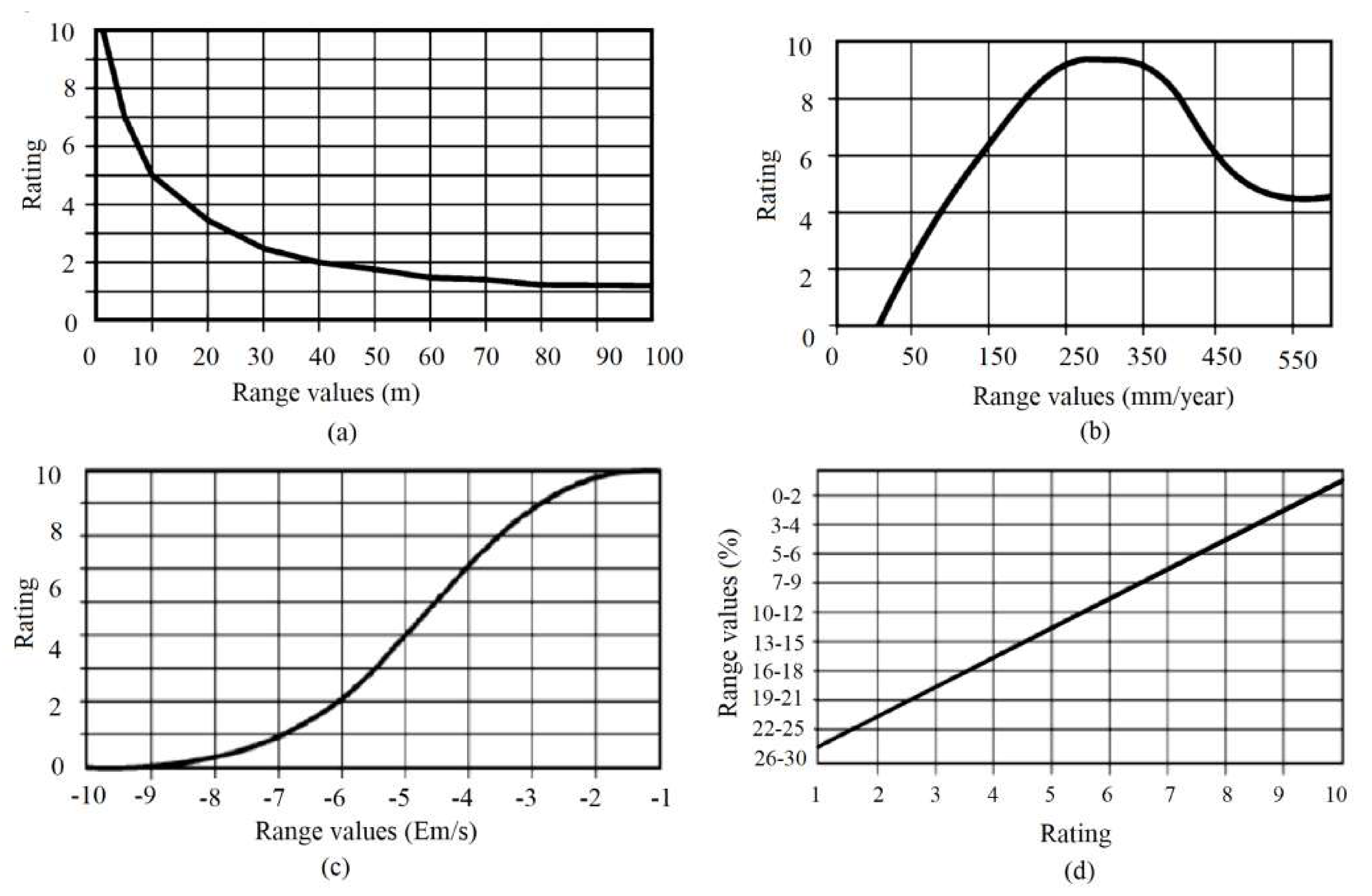
- Assign a rating, P, between 1 and 10, to each subinterval, in concordance with its importance in the last step of the algorithm (Figure 2)
- Choose the strings of weights, W, and multiply the factor ratings (Table 4).
The vulnerability index is computed as a weighted average, by the formula:
being the rating value and is the corresponding weight.
One of the SINTACS advantages is the possibility of simultaneous use in different zones since each situation has assigned a specific weighting rate. Notice the differences between the DRASTIC and SINTACS procedures of weighting and rating, the last one operating in parallel with different strings of weights (Table 4) to describe the environmental conditions [6]. The most difficult task remains the range selection and the assignation of weight and ratings.
Ratings in SINTACS for the net recharge (R) are Coarse alluvial deposit 6–9, karstified limestone 8–10, Fractured limestone 4–8, Fissured dolomite 2–5, Medium-fine alluvial deposit 3–6, sandstone complex 4–7, Sandstone and conglomerate 5–8, Fissured plutonic rock 3–5, Turbidic sequence 2–5, Fissured volcanic rock 5–10, Marl and claystone 1–2, Coarse moraine 4–6, Clay, silt and peat 2–4, Medium –fine moraine 1–2, Pyrolastic rock 2–5, Fissured metamorphic rock 2–6 [27].
The six vulnerability classes (and the corresponding intervals of the vulnerability index) are very high ( 210), high (), moderately high (), medium (), low (), and very low ().
For extending the applicability of SINTACS to the entire Italian territory, a new approach was introduced, by combining the SINTACS Release 5 [28] with the GNDCI_CNR Basic Method [29]. Since its release, SINTACS became one of the most used methods for the assessment of groundwater vulnerability in countries as Algeria, Italy, Jordan, Morocco, Thailand [87,88,89,90,91,92,93].
Corniello et al. [89] remarked that lithological and morphological settings play an important role in the process of generating SINTACS vulnerability maps. In a comparative study of three methods [90] on sites situated in a Mediterranean region, it is shown that the climatic conditions have a significant influence on the methods’ performance, DRASTIC providing better results than SINTACS and AVI. A comparative study of the vulnerability maps produced by DRASTIC and SINTACS for an aquifer situated in Algeria [91] shows that the results are statistically concordant. Luoma et al. [92] emphasize in their research on a coastal aquifer that the SINTACS vulnerability maps are concordant with the field reality.
From the comparative analysis of the results provided by performing DRASTIC, SINTACS, and GOD methods on a database from Central Romania [93], one can remark on the similarity of the maps generated by the first two methods, there are few differences in the extent of the class of low vulnerability. In zones with small vulnerability variations, GOD performed worst. Therefore this method should be used only for regions with big vulnerability variations.
Aiming at detecting the capabilities of five groundwater vulnerability approaches, Civita and De Regibus [11] developed their research in three zones (mountains, hills, and flat). SINTACS and DRASTIC could adapt to the various situations, by comparison to the other competitors (GOD being among them) due to their flexibility.
Secunda et al. [94] and Noori et al. [95] used a SINTACS-LU approach in their research. The new factor, LU, was introduced by analogy to DRASTIC-LU, for considering the land use effect on the groundwater vulnerability. The new approaches better performed than SINTACS in case studies from Israel and Iran. Both SINTACS-LU and DRASTIC-LU vulnerability maps delimited the zones highly affected by human activity [94]. The sensitivity analysis for SINTACS-LU [95] showed that the parameter with the highest impact was the vadose zone, followed by the land use. The analysis of the correlation between the vulnerability index and the nitrate values (recorded on-field) was the highest for SINTACS-LU (0.75), by comparison to those of DRASTIC-LU (0.68) and SI (0.64).
13. Groundwater Vulnerability Assessment to Specific Pollutants
Even if all the described methods could be applied to assess the groundwater vulnerability to contamination, new approaches have been proposed to account for the specific properties of some pollutants. These include Pesticide DRASTIC, Pesticide DRASTIC-LU [38,96], Modified Pesticide DRASTIC [80,81,96], Modified DRASTIC for nitrate [20,46,96,97,98,99]. The factors weights in Pesticide DRASTIC and Pesticide DRASTIC LU differs from those of DRASTIC, the rating being preserved. They are presented in Table 5. The ratings of the land use in Pesticide DRASTIC-LU are 1, 5, 7, or 8.
DRASTIC, Pesticide DRASTIC, and Pesticide DRASTIC-LU were used for a study in a part of the Gangetic Plain with intense agricultural activities. Statistical analysis of the average values revealed that the most significant contribution to calculation the vulnerability indexes were I, T (in DRASTIC and Pesticide DRASTIC), and D, followed by R (in Pesticide DRASTIC LU). The sensitivity analysis found that A and R factors had the highest impact on all the models. The less significant parameters were S, and T—in DRASTIC, I and C—in Pesticide DRASTIC. Pesticide DRASTIC was the best model point of view of the correlation between the field data and prediction [96].
DRASTIC, Pesticide DRASTIC, and SI were applied in a case study of an aquifer from Tunisia. SI and Pesticide DRASTIC better detected the pollution risk. The concordance between the categories of vulnerability determined by these approaches was 64%. The authors [80] recommend the use of these two approaches for different purposes; the first one for monitoring, whereas the second one as a part of a multicriteria decision tool for allocating different zones to specific anthropic activities.
The performance of the same three models, together with Modified DRASTIC were compared on an aquifer in India (Telangana) [81]. The D factor has a considerable impact, followed by soil, the smaller one being that of R. The vulnerability classes are almost the same in SI, modified DRASTIC, and modified Pesticide DRASTIC because of the effect of LU inclusion. The Modified Pesticide DRASTIC map contains a higher area with high vulnerability, compared to Pesticide DRASTIC. The scientists remarked [81] the DRASTIC vulnerability underestimation and SI overestimation. All the models (but SI) are in concordance by at least 60%. It seems that the modified Pesticide DRASTIC provided the best predictions.
The nitrate is not a natural compound of soil, being the result of human activities, like the fertilizers used in agriculture or defecation [100]. While some authors used the Pesticide DRASTIC or Pesticide DRASTIC-LU to study the soil contamination with nitrates [46], other scientists [97,98,99] developed new approaches for improving the weights assigning in DRASTIC. Antonakos and Lambrakis [98] proposed DRASTIC-based hybrid methods, Huan et al. [99] adjusted the DRASTIC rating and weighting system. They validated their models on study cases from Greece and China, respectively.
Kazakis and Voudouris [97] replaced the A, S, and I factors of DRASTIC by the thickness of the aquifer, losses of nitrogen from the soil, and hydraulic resistance. The second factor was estimated by the GLEAMS model [101]. The parameters’ range and weights were also modified. The two new methods, named DRASTIC-PA and DRASTIC-PAN, were compared to DRASTIC and LOSN-PN. Their performance were validated by the sensitivity analysis.
14. Other Approaches
In addition to the discussed approaches and those listed in Introduction [5,12,13,23,24,25,26,27,28,29,30,31,32,33,34,35,36,37], Modified versions of DRASTIC have also been developed. Some of them, for carbonate aquifers, are presented in the articles of Davies et al. [102] (that introduced KARST), Witkowski et al. [103], Różkowski [104], Denny et al. [105] (that introduced DRASTIC-Fm), Jiménez-Madrid et al. [106] (that introduced DRISTPI). We shall not insist here on them, due to lack of space.
As already mentioned, one of the main criticism of DRASTIC was that it does not take into account the study particular characteristics of each study region, and does not adapt the ratings and weights [46]. To surpass this inconvenience, other techniques have been proposed, as follows:
15. Models’ Validation
Different authors used many models to validate the results of the vulnerability maps [25,90,120]. Kumar et al. [21] emphasize that this comparison is not advisable because various approaches use different parameters, so the vulnerability maps might not be similar. The benefit of such procedures is to offer an insight into the existence and spatial distribution of groundwater pollution. Therefore, other techniques should be used, as the validation of the vulnerability maps on contaminants data sets collected on-site from wells distributed in the study region. This is usually done using the concentrations of nitrates in the collected samples. A method whose results are most contrasting could be considered most sensitive, so it can be used [6].
Napolitano-Fabri [121] proposed the single-parameter sensitivity analysis (SPSA), which is the most frequently used technique for evaluating the significance of the parameters in the vulnerability models [46,57,58,64,99,122,123,124,125,126,127]. SPSA provides information on the rating and weighting assigned to each parameter, enabling its evaluation by the researcher. SPSA compares the theoretical and effective weights assigned to each parameter in a model.
Lodwick et al. [128] introduced the map removal sensitivity analysis (MRSA) for assessing the uncertainty degree of the models’ output. MRSA consists of removing one map from the analysis of vulnerability and computing a variation index.
Higher SPSA (MRSA) is, higher the importance of the parameter is.
16. Conclusions
In this article, we reviewed DRASTIC and the main DRASTIC-like approaches proposed by scientists for improving the initial algorithm. The methods for assessment of the groundwater vulnerability in karstic regions were not discussed here. DRASTIC is among the most used tools for groundwater vulnerability evaluation. Generally, it uses readily available geodata with no experimental data. DRASTIC employs numerous parameters, and its outputs are only sometimes compared with field-collected data. Therefore DRASTIC-based forecast should be rigorously checked before making management decisions.
The groundwater vulnerability maps are important tools for assessing the groundwater vulnerability and planning future land use. No method developed for creating vulnerability maps is the most reliable, each of them depending on the aquifer characteristics, the land use, the data availability, the parameters involved in the model, the weightings, and rating assigned to each parameter.
Some aspects should be addressed in the next studies:
- Development of analytical methods for choosing and validating the ratings and weightings attached to each parameter in the models
- Integrating the models of water flow and pollutants’ transport in different soils types in the methodology of choosing the weighting values of different parameters
- Detecting the relationships between the parameters used in the models by statistical methods and removing the effect of this correlation by adjustment of the ratings and weightings attached to the corresponding parameters
- Development of unified models that should include the soil and geological characteristics
- Development of hybrid models to reduce the influence of subjectivity in the parameters’ settings and use the statistical methods for the results’ validation.
- Improvement of the databases containing hydro-chemical elements and their integration into GIS software
- Improvement of GIS software by integrating analytical methods with groundwater vulnerability methods
- Development of spatio-temporal methods for the groundwater vulnerability assessment.
Funding
This research received no external funding.
Conflicts of Interest
The authors declare no conflict of interest.
References
- World Wildlife Fund. Available online: https://www.worldwildlife.org/initiatives/fresh-water (accessed on 15 March 2019).
- Margat, J. Ground Water Vulnerability to Contamination; Bases de la Cartographie, Doc. 68 SGC198 HYD; BRGM: Orleans, France, 1968. (In French) [Google Scholar]
- Hirata, R.; Bertolo, R. Groundwater Vulnerability in Different Climatic Zones. In Encyclopedia of Life Support Systems (EOLSS), Groundwater—Vol. II; Available online: https://www.eolss.net/Sample-Chapters/C07/E2-09-04-06.pdf (accessed on 20 March 2020).
- Ground Water Vulnerability Assessment: Contamination Potential under Conditions of Uncertainty; National Research Council National Academy Press: Washington, DC, USA, 1993; Available online: https://www.nap.edu/read/2050/chapter/3#17 (accessed on 4 September 2019).
- Doerfliger, N.; Jeannin, P.Y.; Zwahlen, F. Water vulnerability assessment in karst environments: A new method of defining protection areas using a multi-attribute approach and GIS tools (EPIK method). Environ. Geol. 1999, 39, 165–176. [Google Scholar] [CrossRef] [Green Version]
- Gogu, R.C.; Dassargues, A. Current trends and future challenges in groundwater vulnerability assessment using overlay and index methods. Environ. Geol. 2000, 39, 549–559. [Google Scholar] [CrossRef]
- Adams, B.; Foster, S.S.D. Land-surface zoning for groundwater protection. Water Environ. J. 1992, 6, 312–319. [Google Scholar] [CrossRef]
- Derouane, J.; Dassargue, A. Delineation of groundwater protection zones based on traces tests and transport modelling in alluvial sediments. Environ. Geol. 1998, 36, 27–32. [Google Scholar] [CrossRef]
- Albinet, M.; Margat, J. Groundwater Pollution Vulnerability Mapping. Bull. Bur. Res. Geol. Min. Bull BRGM 2nd Ser. 1970, 3, 13–22. [Google Scholar]
- Goossens, M.; Van Damme, M. Vulnerability mapping in Flanders, Belgium. In Vulnerability of Soil and Groundwater to Pollutants International Conference; van Duijvenbooden, W., van Waegeningh, G.H., Eds.; Proceedings and Information 38; TNO Committee on Hydrological Research: The Hague, The Netherlands, 1987; pp. 355–360. Available online: https://pascal-francis.inist.fr/vibad/index.php?action=getRecordDetail&lang=en&idt=7424922 (accessed on 23 March 2020).
- Civita, M.; De Regibus, C. Sperimentazione di alcune metodologie per la valutazione della vulnerabilità degli aquiferi. Q Geol. Appl. Pitagora Bologna 1995, 3, 63–71. [Google Scholar]
- Foster, S.S.D. Fundamental concepts in aquifer vulnerability, pollution risk and protection strategy. Hydrol. Resour. Proc. Inf. 1987, 38, 69–86. [Google Scholar]
- Van Stempvoort, D.L.; Evert, L.W. Aquifer vulnerability index: A GIS compatible method for groundwater vulnerability mapping. Can. Water Resour. J. 1993, 18, 25–37. [Google Scholar] [CrossRef] [Green Version]
- Eckhardt, D.A.V.; Stackelberg, P.E. Relation of ground-water quality to land use on Long Island, New York. Ground Water 1995, 33, 1019–1033. [Google Scholar] [CrossRef]
- Masetti, M.; Sterlacchini, S.; Ballabio, C.; Sorichetta, A.; Poli, S. Influence of threshold value in the use of statistical methods for groundwater vulnerability assessment. Sci. Total Environ. 2009, 407, 3836–3846. [Google Scholar] [CrossRef]
- Yen, S.T.; Liu, S.; Kolpin, D.W. Analysis of nitrate in near surface aquifers in the midcontinental United States: An application of the inverse hyperbolic sine tobit model. Water Resour. Res. 1996, 32, 3003–3011. [Google Scholar] [CrossRef]
- Neukum, C.; Hotzl, H.; Himmelsbach, T. Validation of vulnerability mapping methods by field investigations and numerical modelling. Hydrogeol. J. 2008, 16, 641–658. [Google Scholar] [CrossRef]
- Pineros Garcet, J.D.; Ordoñez, A.; Roosen, J.; Vanclooster, M. Metamodelling: Theory, concepts, and application to nitrate leaching modelling. Ecol. Model. 2006, 193, 629–644. [Google Scholar] [CrossRef]
- Singhal, V.; Goyal, R. Development of conceptual groundwater flow model for Pali Area, India. Afr. J. Environ. Sci. Technol. 2011, 5, 1085–1092. [Google Scholar] [CrossRef]
- Fusco, F.; Alloca, V.; Coda, S.; Cusano, D.; Tufano, R.; De Vita, P. Quantitative Assessment of Specific Vulnerability to Nitrate Pollution of Shallow Alluvial Aquifers by Process-Based and Empirical Approaches. Water 2020, 12, 269. [Google Scholar] [CrossRef] [Green Version]
- Kumar, P.; Bansod, K.S.; Debnath, K.S.; Thakur, P.K.; Ghanshyam, C. Index-based groundwater vulnerability mapping models using hydrogeological settings: A critical evaluation. Environ. Impact Assess. Rev. 2015, 51, 38–49. [Google Scholar] [CrossRef]
- Rao, P.S.C.; Alley, W.M. Pesticides. In Regional Groundwater Quality; Alley, W.M., Ed.; Van Nostrand: Reinhold, NY, USA, 1993; pp. 345–382. [Google Scholar]
- Aller, L.; Bennet, T.; Lehr, J.H.; Petty, R.J. DRASTIC: Standardized System for Evaluating Ground Water Pollution Potential using Hydrogeologic Settings; Office of Research Development, US EPA: Ada, OK, USA, 1985. [Google Scholar]
- Ray, I.A.; Odell, P.W. DIVERSITY: A new method for evaluating sensitivity of groundwater to contamination. Environ. Geol. 1993, 22, 344–352. [Google Scholar] [CrossRef]
- Civita, M. Le Carte Della Vulnerabilita Degli Acquiferi all Inquinamento: Teoria e Pratica; Pitagora Editrice: Bologna, Italy, 1994; pp. 325–333. [Google Scholar]
- Civita, M. Legenda Unificata per le Carte Della Vulnerabilita’ dei Corpi Idrici Sotterranei/Unified Legend for the Aquifer Pollution Vulnerability Maps. Studi sulla Vulnerabilita’ degli Acquiferi, 1 (Append.); Pitagora: Bologna, Italy, 1990; p. 13. [Google Scholar]
- Civita, M.; De Maio, M. SINTACS. Un Sistema Parametrico per la Valutazione e la Cartografia Della Vulnerabilita’ Degli Acquiferi All’inquinamento. Metodologia and Automatizzazione; Pitagora: Bologna, Italy, 1997. [Google Scholar]
- Civita, M.; de Maio, M. SINTACS R5-Valutazione e Cartografia Automatica Della Vulnerabilità Degli Acquiferi All’inquinamento con il Sistema Parametrico; Pitagora: Bologna, Italy, 2000; pp. 226–232. [Google Scholar]
- Civita, M. The combined approach when assessing and mapping groundwater vulnerability to contamination. J. Water Resour. Prot. 2010, 2, 14–28. [Google Scholar] [CrossRef] [Green Version]
- Malik, P.; Svasta, J. REKS: An alternative method of Karst groundwater vulnerability estimation. In Proceedings of the XXIX Congress of the International Association of Hydrogeologists, Bratislava, Slovakia, 6–10 September 1999; pp. 79–85. [Google Scholar] [CrossRef]
- Pételet-Giraud, E.; Dörfliger, N.; Crochet, P. RISKE: Méthode d’évaluation multicritère de la vulnérabilité des aquifers karstiques. Application aux systèmes des Fontanilles et Cent-Fonts (Hérault, Sud de la France). Hydrogéol 2000, 4, 71–88. [Google Scholar]
- Plagnes, V.; Théry, S.; Fontaine, L.; Bakalowicz, M.; Dörfliger, N. Karst vulnerability mapping: Improvement of the RISKE method. In Proceedings of the KARST 2005, Water Resources and Environmental Problems in Karst, Belgrade, Serbia, 14–19 September 2005. [Google Scholar]
- Andreo, B.; Ravbar, N.; Vias, J.M. Source vulnerability mapping, in carbonate (karst) aquifers by extension of the COP method: Application to pilot sites. Hydrogeol. J. 2009, 17, 749–758. [Google Scholar] [CrossRef]
- Vías, J.M.; Andreo, B.; Perles, M.J.; Carrasco, F.; Vadillo, I.; Jiménez, P. Proposed method for groundwater vulnerability mapping in carbonate (karstic) aquifers: The COP method. Hydrogeol. J. 2006, 14, 912–927. [Google Scholar] [CrossRef]
- Kavouri, K.; Plagnes, V.; Tremoulet, J.; Dörfliger, N.; Rejiba, F.; Marchet, P. PaPRIKa: A method for estimating karst resource and source vulnerability—Application to the Ouysse karst system (southwest France). Hydrogeol. J. 2011, 19, 339–353. [Google Scholar] [CrossRef]
- Goldscheider, N. Karst groundwater vulnerability mapping: Application of a new method in the Swabian Alb, Germany. Hydrogeol. J. 2005, 13, 555–564. [Google Scholar] [CrossRef]
- Ravbar, N.; Goldscheider, N. Proposed methodology of vulnerability and contamination risk mapping for the protection of karst aquifers in Slovenia. Acta Carsologica 2007, 36, 461–475. [Google Scholar] [CrossRef] [Green Version]
- Aller, L.; Bennett, T.; Lehr, J.H.; Petty, R.J.; Hackett, G. DRASTIC: A Standardized System for Evaluating Groundwater Potential Using Hydrogeologic Settings; EPA/600/2-85/018; U.S. Environmental Protection Agency: Washington, DC, USA, 1987.
- Fan, J.; Oestergaard, K.T.; Guyot, A.; Lockington, D.A. Estimating groundwater recharge and evapotranspiration from water table fluctuations under three vegetation covers in a coastal sandy aquifer of subtropical Australia. J. Hydrol. 2014, 519, 1120–1129. [Google Scholar] [CrossRef] [Green Version]
- Chenini, I.; Zghibi, A.; Kouzana, L. Hydrogeological investigations and groundwater vulnerability assessment and mapping for groundwater resource protection and management: State of the art and a case study. J. Afr. Earth Sci. 2015, 109, 11–26. [Google Scholar] [CrossRef]
- Kalinski, R.J.; Kelly, W.E.; Bogardi, I.; Ehrman, R.L.; Yamamoto, P.O. Correlation between DRASTIC vulnerabilities and incidents of VOC contamination of municipal wells in Nebraska. Groundwater 1994, 32, 31–34. [Google Scholar] [CrossRef]
- McLay, C.D.A.; Dragden, R.; Sparling, G.; Selvarajah, N. Predicting groundwater nitrate concentrations in a region of mixed agricultural land use: A comparison of three approaches. Environ. Pollut. 2001, 115, 191–204. [Google Scholar] [CrossRef]
- Akhavan, S.; Mousavi, S.; Abedi-Koupai, J.; Abbaspour, K.C. Conditioning DRASTIC model to simulate nitrate pollution case study: Hamadan-Bahar plain. Environ. Earth Sci. 2011, 63, 1155–1167. [Google Scholar] [CrossRef] [Green Version]
- Barbash, J.E.; Resek, E.A. Pesticides in Ground Water: Distribution, Trends, and Governing Factors; Ann Arbor Press Inc.: Ann Arbor, MI, USA, 1996. [Google Scholar]
- Jang, W.S.; Engel, B.; Harbor, J.; Theller, L. Aquifer Vulnerability Assessment for Sustainable Groundwater Management Using DRASTIC. Water 2017, 9, 792. [Google Scholar] [CrossRef] [Green Version]
- Neshat, A.; Pradhan, B.; Pirastehm, S.; Shafri, H.Z.M. Estimating groundwater vulnerability to pollution using a modified DRASTIC model in the Kerman agricultural area, Iran. Environ. Earth Sci. 2014, 71, 3119–3131. [Google Scholar] [CrossRef]
- Holden, L.R.; Graham, J.A.; Whitmore, R.W.; Alexander, W.J.; Pratt, R.W.; Liddle, S.F.; Piper, L.L. Results of the national Alachlor well water survey. Environ. Sci. Technol. 1992, 26, 936–943. [Google Scholar] [CrossRef]
- Maas, R.P.; Kucken, D.J.; Patch, S.C.; Peek, B.T.; Van Engelen, D.L. Pesticides in eastern North Caroline rural supply wells: Landuse factors and persistence. J. Environ. Qual. 1995, 24, 426–431. [Google Scholar] [CrossRef]
- Wang, Y.; Merkel, B.J.; Li, Y.; Ye, H.; Fu, S.; Ihm, D. Vulnerability of groundwater in Quaternary aquifers to organic contaminants: A case study in Wuhan City, China. Environ. Geol. 2007, 53, 479–484. [Google Scholar] [CrossRef]
- Merchant, J.W. GIS-Based Groundwater Pollution Hazard Assessment: A Critical Review of the DRASTIC model. Photogramm. Eng. Remote Sens. 1994, 60, 1117–1127. [Google Scholar]
- Alam, F.; Umar, R.; Ahmad, S.; Dar, A.F. A new model (DRASTIC-LU) for evaluating groundwater vulnerability in parts of Central Ganga plain, India. Arab. J. Geosci. 2012, 7, 927–937. [Google Scholar] [CrossRef]
- Merchant, J.W.; Whittemore, D.; Whistler, O.J.L.; McElwee, C.D.; Woods, J.J. Groundwater Pollution Hazard Assessment: A GIS Approach. In Proceedings of the International Geographic Information Systems (IGIS) Symposium, Association of American Geographers, Washington, DC, USA, 15–18 November 1987; Volume 3, pp. 103–115. [Google Scholar]
- Hrkal, Z. Vulnerability of groundwater to acid deposition, Jizerske Mountains, northern Czech Republic: Construction and reliability of a GIS-based vulnerability map. Hydrogeol. J. 2001, 9, 348–357. [Google Scholar] [CrossRef]
- Rupert, M.G. Calibration of the DRASTIC ground water vulnerability mapping method. Ground Water 2001, 39, 625–630. [Google Scholar] [CrossRef]
- Lake, I.R.; Lovett, A.A.; Hiscock, K.M. Evaluating factors influencing groundwater vulnerability to nitrate pollution: Developing the potential of GIS. J. Environ. Manag. 2003, 68, 315–328. [Google Scholar] [CrossRef]
- Babiker, I.S.; Mohammed, M.A.A.; Hiyama, T.; Kato, K. A GIS-based DRASTIC model for assessing aquifer vulnerability in Kakamigahara Heights, Gifu Prefecture, central Japan. Sci. Total Environ. 2005, 345, 127–140. [Google Scholar] [CrossRef]
- Dixon, B. Groundwater vulnerability mapping: A GIS and fuzzy rule based integrated tool. Appl. Geogr. 2005, 25, 327–347. [Google Scholar] [CrossRef]
- Rahman, A. A GIS based DRASTIC model for assessing groundwater vulnerability in shallow aquifer in Aligarh, India. Appl. Geogr. 2008, 28, 32–53. [Google Scholar] [CrossRef]
- Shirazi, S.M.; Imran, H.M.; Akib, S.; Yusop, Z.; Harun, Z.B. Groundwater vulnerability assessment in the Melaka State of Malaysia using DRASTIC and GIS techniques. Environ. Earth Sci. 2013, 70, 2293–2304. [Google Scholar] [CrossRef]
- Thirumalaivasan, D.; Karmegam, M.; Venugopal, K. AHP-DRASTIC: Software for specific aquifer vulnerability assessment using DRASTIC model and GIS. Environ. Model. Softw. 2003, 18, 645–656. [Google Scholar] [CrossRef]
- Sener, E.; Sener, S.; Davraz, A. Assessment of aquifer vulnerability based on GIS and DRASTIC methods: A case study of the Senirkent-Uluborlu Basin (Isparta, Turkey). Hydrogeol. J. 2009, 17, 2023. [Google Scholar] [CrossRef]
- Ariffin, S.M.; Zawawi, M.A.M.; Man, H.C. Evaluation of groundwater pollution risk (GPR) from agricultural activities using DRASTIC model and GIS. In IOP Conference Series: Earth and Environment Science; IOP Publishing: Bristol, UK, 2016; Volume 37, p. 012078. [Google Scholar] [CrossRef] [Green Version]
- Mendoza, J.A.; Barmen, G. Assessment of groundwater vulnerability in the Rıo Artiguas basin, Nicaragua. Environ. Geol. 2006, 50, 569–580. [Google Scholar] [CrossRef]
- Saidi, S.; Bouri, S.; Dhia, H.B. Groundwater vulnerability and risk mapping of the Hajeb-jelma aquifer (Central Tunisia) using a GIS-based DRASTIC model. Environ. Earth Sci. 2010, 59, 1579–1588. [Google Scholar] [CrossRef]
- Castany, G. Principe et Methodes de L’hydrogeologie; Dunod: Paris, France, 1982. [Google Scholar]
- Sakala, E.; Fourie, F.; Gomo, M.; Coetzee, H.; Magadaza, L. Specific groundwater vulnerability mapping: Case study of acid mine drainage in the Witbank coalfield, South Africa. In Proceedings of the Sixth IASTED International Conference, Gaborone, Botswana, 5–7 September 2016. [Google Scholar] [CrossRef] [Green Version]
- Zhou, J.; Li, G.; Liu, F.; Wang, Y.; Guo, X. DRAV model and its application in assessing groundwater vulnerability in arid area: A case study of pore phreatic water in Tarim Basin, Xinjiang, Northwest China. Environ. Earth Sci. 2010, 60, 1055–1063. [Google Scholar] [CrossRef]
- Singh, A.; Srivastav, S.K.; Kumar, S.; Chakrapani, G.J. A modified-DRASTIC model (DRASTICA) for assessment of groundwater vulnerability to pollution in an urbanized environment in Lucknow, India. Environ. Earth Sci. 2015, 74, 5475–5490. [Google Scholar] [CrossRef]
- Amadi, N.; Olasehinde, P.I.; Nwankwoala, H.O.; Dan-Hassan, M.A.; Okoye, N.O. Aquifer vulnerability studies using DRASTICA Model. Int. J. Eng. Sci. Invent. 2014, 3, 1–10. [Google Scholar]
- Hussain, M.H.; Singhai, D.C.; Joshi, H.; Kumar, S. Assessment of groundwater vulnerability in tropical alluvial interfluves, India. Bhu-Jal News J. 2006, 1–4, 31–43. [Google Scholar]
- Khan, M.M.A.; Umar, R.; Lateh, H. Assessment of aquifer vulnerability in parts of Indo Gangetic plain, India. Int. J. Phys. Sci. 2010, 5, 1711–1720. [Google Scholar]
- Kumar, A.; Khrisma, A.K. Groundwater vulnerability and contamination risk assessment using GIS-based modified DRASTIC-LU model in hard rock aquifer system in India. Geocarto Int. 2019. [Google Scholar] [CrossRef]
- Sinha, M.K.; Verma, M.K.; Ahmad, I.; Baier, K.; Jha, R.; Azzam, R. Assessment of groundwater vulnerability using modified DRASTIC model in Kharun Basin, Chhattisgarh, India. Arab. J. Geosci. 2016, 9, 11–22. [Google Scholar] [CrossRef]
- Umar, R.; Ahmed, I.; Alam, F. Mapping Groundwater Vulnerable Zones Using Modified DRASTIC Approach of an Alluvial Aquifer in Parts of Central Ganga Plain, Western Uttar Pradesh. J. Geol. Soc. India 2009, 73, 193–201. [Google Scholar] [CrossRef]
- Qinghai, G.; Yanxin, W.; Xubo, G.; Teng, M. A new model (DRARCH) for assessing groundwater vulnerability to arsenic contamination at basin scale: A case study in Taiyuan basin, northern China. Environ. Geol. 2007, 52, 923–932. [Google Scholar] [CrossRef]
- Ribeiro, L. SI: A New Index of Aquifer Susceptibility to Agricultural Pollution; ERSHA/CVRM, Instituto Superior Técnico: Lisboa, Portugal, 2000. [Google Scholar]
- Stigter, T.Y.; Riberio, L.; Dill, A.M.M.C. Evaluation of an intrinsic and a specific vulnerability assessment method in comparison with groundwater salinization and nitrate contamination levels in two agricultural regions in the south of Portugal. Hydrogeol. J. 2006, 14, 79–99. [Google Scholar] [CrossRef]
- Ribeiro, L.; Pindo, J.C.; Dominguez-Granda, L. Assessment of groundwater vulnerability in the Daule aquifer, Ecuador, using the susceptibility index method. Sci. Total Environ. 2017, 574, 1674–1683. [Google Scholar] [CrossRef]
- Anane, M.; Abidi, B.; Lachaal, F.; Limam, A.; Jellali, S. GIS-based DRASTIC, Pesticide DRASTIC and the Susceptibility Index (SI): Comparative study for evaluation of pollution. Hydrogeol. J. 2013, 21, 715–731. [Google Scholar] [CrossRef]
- Brindha, K.L.E. Cross comparison of five popular groundwater pollution vulnerability index approaches. J. Hydrol. 2015, 524, 597–613. [Google Scholar] [CrossRef]
- El Himer, H.; Fakir, Y.; Stigter, T.Y.; Lepage, M.; El Mandour, A.; Ribeiro, L. Assessment of the vulnerability to pollution of a wetland watershed. The case study of Oualidia-Sidi Moussa wetland, Morocco. Aquat. Ecosyst. Health 2013, 16, 205–215. [Google Scholar] [CrossRef]
- Hamza, M.H.; Added, A. Validity of DRASTIC and SI vulnerability methods. In GeoSpatial Visual Analytics: Geographical Information Processing and Visual Analytics for Environmental Security; De Amicis, R., Stojanovic, R., Conti, G., Eds.; Springer: Dordrecht, The Netherlands, 2009; pp. 395–407. [Google Scholar]
- Hamza, M.H.; Added, A.; Francés, A.; Rodríguez, R. Validité de l’application des méthodes de vulnérabilité DRASTIC, SINTACS et SI à l’étude de la pollution par les nitrates dans la nappe phréatique de Metline–Ras Jebel–Raf Raf (Nord-Est tunisien). Comptes Rendus Geosci. 2007, 339, 493–505. [Google Scholar] [CrossRef]
- Teixeira, J.; Chaminé, H.I.; Marques, J.E.; Carvalho, J.M.; Pereira, A.J.S.C.; Carvalho, M.R.; Fonseca, P.E.; Pérez-Alberti, A.; Rocha, F. A comprehensive analysis of groundwater resources using GIS and multicriteria tools (Caldas da Cavaca, Central). Environ. Earth Sci. 2014, 73. [Google Scholar] [CrossRef]
- Rana, S.; Kumar, P.; Puri, S.; Bansod, B.K.; Debnath, S.; Ghanshyam, C.; Kapur, P. Localization of Arsenic Contaminated Zone of Domkal Block in Murshidabad, West Bengal using GIS-based DRASTIC model. In Proceedings of the International Conference on Communication and Computing (ICC-2014), Bangalore, India, 10–14 June 2014. [Google Scholar] [CrossRef]
- Narany, T.; Ramli, M.F.; Aris, A.Z.; Sulaiman, W.N.A.; Fakharian, K. Spatial assessment of groundwater quality monitoring wells using indicator kriging and risk mapping, Amol-Babol Plain, Iran. Water 2013, 6, 68–85. [Google Scholar] [CrossRef] [Green Version]
- Boufekane, A.; Saighi, O. Assessment of groundwater pollution by nitrates using intrinsic vulnerability methods: A case study of the Nil valley groundwater (Jijel, North-East Algeria). Afr. J. Environ. Sci. Technol. 2013, 7, 949–960. [Google Scholar] [CrossRef]
- Al Kuisi, M.; El-Naqa, A.; Hammouri, N. Vulnerability mapping of shallow groundwater aquifer using SINTACS model in the Jordan Valley area, Jordan. Environ. Geol. 2006, 50, 651–667. [Google Scholar] [CrossRef]
- Corniello, A.; Ducci, D.; Monti, G.M. Aquifer pollution vulnerability in the Sorrento Peninsula, Southern Italy, evaluated by SINTACS Method. Geofís. Int. 2004, 43, 575–581. [Google Scholar]
- Draoui, M.; Vias, J.; Andreo, B.; Targuisti, K.; El Messari, J.S. A Comparative Study of Four Vulnerability Mapping Methods in a Detritic Aquifer under Mediterranean Climatic Conditions. Environ. Geol. 2008, 54, 455–463. [Google Scholar] [CrossRef]
- Kaddour, K.; Houcine, B.; Smail, M. Assessment of the vulnerability of an aquifer by DRASTIC and SYNTACS methods: Aquifer of Bazer—Geult Zerga area (northeast Algeria). E3 J. Environ. Res. Manag. 2014, 5, 0169–0179. [Google Scholar]
- Majandang, J.; Sarapirome, S. Groundwater vulnerability assessment and sensitivity analysis in Nong Rua, Khon Kaen, Thailand, using a GIS-Based SINTACS Model. Environ. Earth Sci. 2013, 68, 2025–2039. [Google Scholar] [CrossRef]
- Gogu, R.C.; Pandele, A.; Ionita, A.; Ionescu, C. Groundwater vulnerability analysis using a low-cost Geographical Information System. In Proceedings of the MIS/UDMS Conference WELL-GIS WORKSHOP’s Environmental Information Systems for Regional and Municipal Planning, Prague, Czech Republic, 20 November 1996; pp. 35–49. [Google Scholar]
- Secunda, S.; Collin, M.; Melloul, A.J. Groundwater Vulnerability Assessment Using a Composite Model Combining DRASTIC with Extensive Land Use in Israel’s Sharon Region. J. Environ. Manag. 1998, 54, 39–57. [Google Scholar] [CrossRef]
- Noori, R.; Ghahremanzadeh, H.; Kløve, B.; Adamowski, F.J.; Baghvand, A. Modified-DRASTIC, modified-SINTACS and SI methods for groundwater vulnerability assessment in the southern Tehran aquifer. J. Environ. Sci. Health 2019, 54, 89–91. [Google Scholar] [CrossRef] [PubMed]
- Saha, D.; Alam, F. Groundwater vulnerability assessment using DRASTIC and Pesticide DRASTIC models in intense agriculture area of the Gangetic plains, India. Environ. Monit. Assess. 2014, 186, 8741–8763. [Google Scholar] [CrossRef]
- Kazakis, N.; Voudouris, K.S. Groundwater vulnerability and pollution risk assessment of porous aquifers to nitrate: Modifying the DRASTIC method using quantitative parameters. J. Hydrol. 2015, 525, 13–25. [Google Scholar] [CrossRef]
- Antonakos, K.; Lambrakis, N.L. Development and testing of three hybrid methods for assessment of aquifer vulnerability to nitrates, based on the DRASTIC model, an example from NE Korinthia, Greece. J. Hydrol. 2007, 333, 288–304. [Google Scholar] [CrossRef]
- Huan, H.; Wang, J.; Teng, Y. Assessment and validation of groundwater vulnerability to nitrate based on a modified DRASTIC model: A case study in Jilin City of northeast China. Sci. Total Environ. 2012, 440, 14–23. [Google Scholar] [CrossRef] [PubMed]
- Javadi, S.; Kavehkar, N.; Mohammadi, K.; Khodadadi, A.; Kahawita, R. Calibrating DRASTIC using field measurements sensitivity analysis and statistical methods to assess groundwater vulnerability. Water Int. 2011, 36, 719–732. [Google Scholar] [CrossRef]
- Harmel, D.; Knisel, W.; Leonard, R.; Davis, F. Groundwater Loading Effects of Agricultural Management Systems. Available online: https://www.ars.usda.gov/plains-area/temple-tx/grassland-soil-and-water-research-laboratory/docs/gleams/ (accessed on 26 April 2020).
- Davis, A.D.; Long, A.J.; Wireman, M. KARSTIC: A sensitivity method for carbonate aquifers in karst terrain. Environ. Geol. 2002, 42, 65–72. [Google Scholar] [CrossRef]
- Witkowski, A.J.; Rubin, K.; Kowalczyk, A.; Różkowski, A.; Wróbel, J. Groundwater vulnerability map of the Chrzanów karst-fissured Triassic aquifer (Poland). Environ. Geol. 2003, 44, 59–67. [Google Scholar] [CrossRef]
- Różkowski, J. Evaluation of intrinsic vulnerability of an Upper Jurassic karst-fissured aquifer in the Jura Krakowska (southern Poland) to anthropogenic pollution using the DRASTIC method. Geol. Q. 2007, 51, 17–26. Available online: https://gq.pgi.gov.pl/article/view/7434 (accessed on 13 January 2020).
- Denny, S.C.; Allen, D.M.; Journeay, J.M. DRASTIC-Fm: A modified vulnerability mapping method for structurally-controlled aquifers. Hydrogeol. J. 2007, 15, 483–494. [Google Scholar] [CrossRef]
- Jiménez-Madrid, A.; Carrasco, F.; Martínez, C.; Gogu, R.C. DRISTPI, A new groundwater vulnerability mapping method for use in karstic and non-karstic aquifers. Q. J. Eng. Geol. Hydroeol. 2013, 46, 245–255. [Google Scholar] [CrossRef]
- Pacheco, F.A.L.; Pires, L.M.G.R.; Santos, R.M.B.; Sanches Fernandes, L.F. Factor weighting in DRASTIC modeling. Sci. Total Environ. 2015, 505, 474–486. [Google Scholar] [CrossRef]
- Hailin, Y.; Ligang, X.; Chang, Y.; Jiaxing, X. Evaluation of groundwater vulnerability with improved DRASTIC method. Procedia Environ. Sci. 2011, 10, 2690–2695. [Google Scholar] [CrossRef] [Green Version]
- Sener, E.; Davraz, A. Assessment of groundwater vulnerability based on a modified DRASTIC model, GIS and an analytic hierarchy process (AHP) method: The case of Egirdir Lake basin (Isparta, Turkey). Hydrogeol. J. 2013, 21, 701–714. [Google Scholar] [CrossRef]
- Shouyu, C.; Guangtao, F. A DRASTIC-based fuzzy pattern recognition methodology for groundwater vulnerability evaluation. Hydrol. Sci. J. 2003, 48, 211–220. [Google Scholar] [CrossRef]
- Afshar, A.I.; Marino, M.A.; Asce, H.M.; Ebtehaj, M.; Moosa Vi, J. Rule-based fuzzy system for assessing groundwater vulnerability. J. Environ. Eng. 2007, 133, 532–540. [Google Scholar] [CrossRef]
- Bojórquez-Tapia, L.A.; Cruz-Bello, G.M.; Luna-González, L.; Juárez, L.; Ortiz-Pérez, M.A. V-DRASTIC: Using visualization to engage policymakers in groundwater vulnerability assessment. J. Hydrol. 2009, 373, 242–255. [Google Scholar] [CrossRef]
- Pathak, D.R.; Hiratsuka, A. An integrated GIS based fuzzy pattern recognition model to compute the groundwater vulnerability index for decision making. J. Hydro-Environ. Res. 2011, 5, 63–77. [Google Scholar] [CrossRef]
- Rezaei, F.; Safavi, H.R.; Ahmadi, A. Groundwater vulnerability assessment using fuzzy logic: A case study in the Zayandehrood Aquifers, Iran. Environ. Manag. 2013, 51, 267–277. [Google Scholar] [CrossRef]
- Fijani, E.; Nadiri, A.; Moghaddam, A.A.; Dixon, B. Optimization of DRASTIC Method by Supervised Committee Machine Artificial Intelligence to Assess Groundwater Vulnerability for Maragheh-Bonab Plain Aquifer, Iran. J. Hydrol. 2013, 503, 89–101. [Google Scholar] [CrossRef]
- Barzegar, R.; Moghaddam, A.A. Combining the advantages of neural networks using the concept of committee machine in the groundwater salinity prediction. Model. Earth Sys. Environ. 2016, 2, 26. [Google Scholar] [CrossRef] [Green Version]
- Barzegar, R.; Moghaddam, A.A.; Baghban, H. A supervised committee machine artificial intelligent for improving DRASTIC method to assess groundwater contamination risk: A case study from Tabriz plain aquifer, Iran. Stoch. Environ. Res. Risk Assess. 2016, 30, 883–899. [Google Scholar] [CrossRef]
- Panagopoulos, G.P.; Antonakos, A.K.; Lambrakis, N.J. Optimization of the DRASTIC method for groundwater vulnerability assessment via the use of simple statistical methods and GIS. Hydrogeol. J. 2006, 14, 894–911. [Google Scholar] [CrossRef]
- Neshat, A.; Pradhan, B.; Shafri, H.Z.M. An integrated GIS based statistical model to compute groundwater vulnerability index for decision maker in agricultural area. J. Indian Soc. Remote Sens. 2014, 42, 777–788. [Google Scholar] [CrossRef]
- Ghazavi, R.; Ebrahimi, Z. Assessing groundwater vulnerability to contamination in an arid environment using DRASTIC and GOD models. Int. J. Environ. Sci. Technol. 2015, 12, 2909–2918. [Google Scholar] [CrossRef] [Green Version]
- Pacheco, F.A.L.; Sanches Fernandes, L.F. The multivariate statistical structure of DRASTIC model. J. Hydrol. 2013, 476, 442–459. [Google Scholar] [CrossRef]
- Napolitano, P.; Fabbri, A.G. Single parameter sensitivity analysis for aquifer vulnerability assessment using DRASTIC and SINTACS. In Proceedings of the HydroGIS: Application of Geographical Information Systems in Hydrology and Water Resources Management; Kovar, K., Nachtnebel, H.P., Eds.; IAHS Publication no. 235; IAHS: Wallingford, UK, 1996; pp. 559–566. [Google Scholar]
- Neshat, A.; Pradhan, B.; Dadras, M. Groundwater vulnerability assessment using an improved DRASTIC method in GIS. Resour. Conserv. Recycl. 2014, 86, 74–86. [Google Scholar] [CrossRef]
- Al-Hanbali, A.; Kondoh, A. Groundwater vulnerability assessment and evaluation of human activity impact (HAI) within the Dead Sea groundwater basin, Jordan. Hydrogeol. J. 2008, 16, 499–510. [Google Scholar] [CrossRef]
- Almasri, M.N. Assessment of intrinsic vulnerability to contamination for Gaza coastal aquifer, Palestine. J. Environ. Manag. 2008, 88, 577–593. [Google Scholar] [CrossRef]
- Hasiniaina, F.; Zhou, J.; Guoyi, L. Regional assessment of groundwater vulnerability in Tamtsag basin, Mongolia using drastic model. J. Am. Sci. 2010, 6, 65–78. [Google Scholar]
- Samake, M.; Tang, Z.; Hlaing, W.; M’Bue, I.; Kasereka, K. Assessment of groundwater pollution potential of the Datong Basin, Northern China. J. Sustain. Dev. 2010, 3, 140–152. [Google Scholar] [CrossRef] [Green Version]
- Lodwik, W.A.; Monson, W.; Svoboda, L. Attribute error and sensitivity analysis of maps operation in geographical information systems-sustainability analysis. Int. J. Geogr. Inf. Syst. 1990, 4, 413–428. [Google Scholar] [CrossRef]
Figure 1.
Flowchart for building a vulnerability map in DRASTIC (adapted from [61]).
Figure 1.
Flowchart for building a vulnerability map in DRASTIC (adapted from [61]).

Figure 2.
Ratings in SINTACS for (a) S, (b) I, (c) C, (d) S parameters (adapted from [29]).
Figure 2.
Ratings in SINTACS for (a) S, (b) I, (c) C, (d) S parameters (adapted from [29]).


Table 1.
Methods and corresponding parameters for groundwater vulnerability assessment.
| Parameter/Method | Depth to the Water Table | Net Recharge | Hydrogeological Features | Soil Characteristics | Topographic Slope | Characteristics of Unsaturated Zone | Aquifer Hydraulic Conductivity | Liniment Density | Stream Network | Aquifer Tickness | Landuse # | Anthropogenic ## Impact (LU) | Pesticides | Specific Region |
|---|---|---|---|---|---|---|---|---|---|---|---|---|---|---|
| DRASTIC | x | x | x | x | x | x | x | |||||||
| DRASTICM | x | x | x | x | x | x | x | x | ||||||
| DRIST | x | x | x | x | x | x | ||||||||
| DRAV | x | x | x | * | ||||||||||
| DRAMIC | x | x | x | x | ** | x | x | |||||||
| DRASTICA | x | x | x | x | x | x | x | |||||||
| DRASTIC-LU | x | x | x | x | x | x | x | x | ||||||
| DRASIC-LU | x | x | x | x | x | x | x | |||||||
| SI | x | x | x | x | x | x | ||||||||
| DRARCH | x | x | *** | x | x | x | ||||||||
| SINTACS | x | x | x | x | x | x | x | x | x | x | ||||
| SINTACS-LU | x | x | x | x | x | x | x | x | x | x | x | |||
| Pesticide DRASTIC | x | x | x | x | x | x | x | x | ||||||
| Pesticide DRASTIC LU | x | x | x | x | x | x | x | x | x |
# The land use parameter characterize the human activity as effect on the runoff coefficient, not as the contaminants’ nature. ## Refers to the impact of the human activity as impact of the built environment or the nature of pollutant. * replaced by the vadose zone lithology. ** replaced by the contaminant impact. *** replaced by the ratio of the clay layers’ thickness to the vadose zone thickness.
Table 2.
DRASTIC D, R, T, and C rating and weighting [38].
Table 2.
DRASTIC D, R, T, and C rating and weighting [38].
| Depth to Water (mm) − weight = 5 | |||||||
| range | 0–1.5 | 1.5–4.6 | 4.6–9.1 | 9.1–15.2 | 15.2–22.8 | 22.8–30.4 | >30.4 |
| rating | 10 | 9 | 7 | 5 | 3 | 2 | 1 |
| Net Recharge (mm) − weight = 4 | |||||||
| range | 0–50.8 | 50.8–101.6 | 101.6–177.8 | 177.8–254 | >254 | ||
| rating | 1 | 3 | 7 | 8 | 9 | ||
| Hydraulic Conductivity of the Aquifer (m/day) − weight = 3 | |||||||
| range | 0.04–4.1 | 4.1–12.3 | 12.3–28.7 | 28.7–41 | 41–82 | >82 | |
| rating | 1 | 2 | 4 | 6 | 8 | 10 | |
| Topography (slope %) − weight = 1 | |||||||
| range | 0–2 | 2–6 | 6–12 | 12–18 | >18 | ||
| rating | 10 | 9 | 5 | 3 | 1 | ||
Table 3.
DRASTIC A, I, S rating and weighting
| Aquifer Media | Vadose Zone Material | Soil Media | |||
|---|---|---|---|---|---|
| weight = 3 | rating | weight = 5 | rating | weight = 2 | rating |
| Massive shale | 2 | Silt/clay | 1 | Non-srinking and non-aggregated clay | 1 |
| Metamorphic/igneous | 3 | Shale | 3 | Muck | 2 |
| Weathered metamorphic/igneous | 4 | Metamorphic/igneous | 4 | Clay loam | 3 |
| Thin-bedded sandstone, limestone, shale sequences | 6 | Limestone | 6 | Silty loam | 4 |
| Massive sandstone | 6 | Sandstone | 6 | Loam | 5 |
| Massive limestone | 8 | Bedded limestone, Sandstone, shale | 6 | Sandy loam | 6 |
| Sand and gravel | 8 | Sand and gravel with significant silt and clay | 6 | Shrinking and/or aggregated clay | 7 |
| Basalt | 9 | Sand and gravel | 8 | Peat | 8 |
| Karst limestone | 10 | Basalt | 9 | Sand | 9 |
| Karst limestone | 10 | Gravel | 10 | ||
| Thin or absent | 10 | ||||
Table 4.
Strings of weights in SINTACS (adapted from [29]).
Table 4.
Strings of weights in SINTACS (adapted from [29]).
| Parameter | S | I | N | T | A | C | S |
|---|---|---|---|---|---|---|---|
| Normal | 5 | 4 | 5 | 3 | 3 | 3 | 3 |
| Severe | 5 | 5 | 4 | 5 | 3 | 2 | 2 |
| Seepage | 4 | 4 | 4 | 2 | 5 | 5 | 2 |
| Karst | 2 | 5 | 1 | 3 | 5 | 5 | 5 |
| Fissured | 3 | 3 | 3 | 4 | 4 | 5 | 4 |
| Nitrates | 5 | 5 | 4 | 5 | 2 | 2 | 3 |
Table 5.
Weights assigned to the parameters in Pesticide DRASTIC, Pesticide DRASTIC-LU.
| Parameter | D | R | A | S | T | I | C | LU |
|---|---|---|---|---|---|---|---|---|
| Pesticide DRASTIC | 5 | 4 | 3 | 5 | 3 | 4 | 2 | - |
| Pesticide DRASTIC-LU | 5 | 4 | 3 | 5 | 3 | 4 | 2 | 5 |
© 2020 by the author. Licensee MDPI, Basel, Switzerland. This article is an open access article distributed under the terms and conditions of the Creative Commons Attribution (CC BY) license (http://creativecommons.org/licenses/by/4.0/).
Share and Cite
MDPI and ACS Style
Barbulescu, A. Assessing Groundwater Vulnerability: DRASTIC and DRASTIC-Like Methods: A Review. Water 2020, 12, 1356. https://doi.org/10.3390/w12051356
AMA Style
Barbulescu A. Assessing Groundwater Vulnerability: DRASTIC and DRASTIC-Like Methods: A Review. Water. 2020; 12(5):1356. https://doi.org/10.3390/w12051356
Chicago/Turabian StyleBarbulescu, Alina. 2020. "Assessing Groundwater Vulnerability: DRASTIC and DRASTIC-Like Methods: A Review" Water 12, no. 5: 1356. https://doi.org/10.3390/w12051356
Note that from the first issue of 2016, this journal uses article numbers instead of page numbers. See further details here.