Machine Learning Methods for Improved Understanding of a Pumping Test in Heterogeneous Aquifers

Abstract

Pumping tests are very important means for investigating aquifer properties; however, interpreting the data using common analytical solutions become invalid in complex aquifer systems. The paper aims to explore the potential of machine learning methods in retrieving the pumping tests information in a field site in the Democratic Republic of Congo. A newly planned mining site with a pumping test of three pumping wells and 28 observation wells over one month was chosen to analyze the significance of machine learning methods in the pumping test analysis. Widely used machine learning methods, including correlation, cluster, time-series analysis, artificial neural network (ANN), support vector machine (SVR), random forest (RF) method, and linear regression, are all used in this study. Correlation and cluster analyses among wells provide visual pictures of possible hydraulic connections. The pathway with the best permeability ranges from the depth of 250 m to 350 m. Time-series analysis perfectly captured changes of drawdowns within the three pumping wells. The RF method is found to have the higher accuracy and the lower sensitivity to model parameters than ANN and SVR methods. The coupling of the linear regressive model and analytical solutions is applied to estimate hydraulic conductivities. The results found that ML methods can significantly and effectively improve our understanding of pumping tests by revealing inherent information hidden in those tests.

1. Introduction

Groundwater is one of the most valuable natural resources, and accounts for over 66% of freshwater resources in the world [1]. Pumping tests play an important role in aquifer property estimations and groundwater resource evaluations. Different analytical solutions [2], such as Theis solutions for confined aquifers and Hantush-Jacob solutions for leaky aquifers, have been developed to provide methods to interpret pumping test data. However, these solutions may become invalid in complex hydrogeological conditions, due to the limitation of their strict assumptions. It is highly necessary to seek an alternative method to retrieve the hidden information about the relationship between the wells behind pumping tests.

In the context of the complexity of a groundwater system in heterogeneous aquifers, machine learning methods have been progressively and successfully applied in groundwater studies [3], including groundwater level forecasting [4,5,6,7], parameter estimation [8,9,10,11] or optimization [12,13] for groundwater models, downscaling of coarse Gravity Recovery and Climate Experiment (GRACE) data [14], development of surrogate models [15], risk assessment of groundwater contamination [16], chemical reactions [17], and well placement evaluation [18]. The employed machine learning (ML) methods mainly include artificial neural networks (ANNs), genetic programming, neuro-fuzzy theory, autoregressive models, support vector machine (SVM) and random forest (RF) methods, and boosted regression tree method. ML methods depend on the selected variables, and thus groundwater modelers may overlook the significance of non-physical-based ML methods. However, physical-based models for pumping tests are challenging, due to the uncertainties of hydrogeology parameters, high time costs, and complex boundary conditions. After numerical model calibration, the outputs from the model serve as the inputs for ML methods to develop surrogate models, which become computationally inexpensive alternatives for numerical models. Meanwhile, with limited hydrogeological information, existing parameter estimations are not enough to support the accurate simulation of numerical models. ML methods provide quick analysis of hidden correlations, and thus are necessary tools for hydrogeological studies.

The Kolwezi megabreccia in the Democratic Republic of Congo (DRC) contains Cu–Co deposits hosted in folded and brittle-fractured structures of the Mines Subgroup [19]. A newly planned underground mine in the Kolwezi Copper Deposit was chosen as the study area. The syncline strata in the mine are overturned with complex geologic and hydrogeological conditions. To analyze the hydrogeological conditions of the mining area and accurately estimate the properties of the mine geology, a large pumping test, including three pumping wells and 28 observation wells, over the period of one month was carried out by North China Engineering Investigation Institute Co., Ltd. The contour maps are not sufficient to demonstrate the change pattern of drawdowns in the pumping tests. Meanwhile, there have been very limited studies on pumping tests using ML methods until now. Therefore, the objectives of this paper are to fully explore the changes of groundwater levels induced by a pumping test using statistical analysis and ML methods. The focused contents include (1) correlation analysis of drawdown changes over the entire period of pumping and recovery for 28 observation wells, (2) forecasting of groundwater level in pumping wells using time-series methods; (3) model development for estimating groundwater level changes induced by pumping using multiple ML methods. The innovative point of this study lies in exploring the potential of ML methods in the studies of pumping tests.

2. Materials and Methods

2.1. Study Area

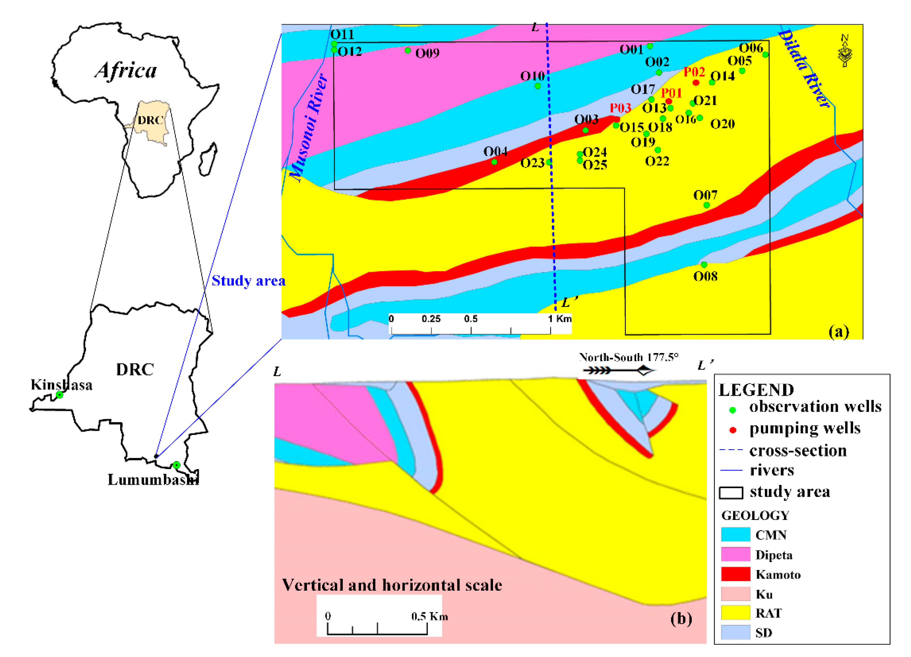
The study area is located at the south of the equator in the Katanga plateau of the DRC (Figure 1a). The study area has a savanna climate. The annual mean temperature is approximately 21.2 ℃. The average annual precipitation from 1979 to 2017 was approximately 1144.90 mm, and the average annual evaporation was approximately 1860.00 mm. Precipitation mainly happens from November to March of the following year, which accounts for more than 85% of the annual precipitation. The dry season is from May to September, with low monthly precipitation of less than 5 mm. The overall terrain is high in the south and low in the north, with varying elevations from 1250 m to 1550 m. The nearest rivers are the Musonoi River and the Dilala River. The Musonoi River flows towards the north. The Dilala River surrounds the east and north sides of the mining area, and finally joins the Musonoi River in the northwest of the mining area. According to an investigation by the North China Engineering Investigation Institute Co., Ltd., the linkage between the Musonoi River and groundwater is weak. Due to the lack of continuous monitoring of flow rate of these two rivers, the influences of the river on groundwater levels will not be evaluated in this study.

The strata in the study area are of the Late Proterozoic Katanga supergroup, which can be subdivided into the upper Kundelungu group and the lower Roan group (host strata). The strata in this area are mainly the Katanga series and the quaternary. The Katanga series mainly includes the Roan group (R), the Nguba group (Ng), and the Kundelungu group (Ku). A cross-section can be shown in Figure 1b [20]. The series of geology from young to old can be seen in

Table 1. List of regional stratigraphy in the study area.

Series (From Young to Old)	Formation		Local Name	Brief Description	Approximated Thickness (m)
Kundelungu	Kundelungu		Ku	Sediments	3000–5000
Nguba	Nguba		Ng	Sandstone, shale	200–500
Upper Roan (R)	R4		Mwashya	shale, siltstone, sandstone, dolomites	50–100
	R3-2		Dipeta	Sandy shales	about 1000
	R3-1		Roches Greseuse Superior (RGS)	Grey shales	100–200
Lower Roan	R2-3	Mines Group	Calcaire á Minerals Noirs (CMN)	Black calcareous siltstone	130
	R2-2		Schistes Dolomitic Superior (SDS)	Dolomitic shales, black ore mineral zone (BOMZ)	50–80
	R2-1		Schistes de Base (SDB)	Dolomitic shales, black ore mineral zone (BOMZ)	10–15
			Roches Silicieuses Cellulaire (RSC)	Siliceous, vuggy dolomite	12–25
			Roches Silicieuses Feuilletees (RSF)	Bedded dolomitic siltstone	5
			Dolomie Stratifiee (DSTRAT)	Grey talcose sandstone	3
			Roches Argileuses Talceuse (RAT) GRISES	Grey talcose sandstone	2–5
	R1		Roches Argileuses Talceuse (RAT2)	Talcose sandstone	190
			Roches Argileuses Talceuse (RAT1)	Talcose sandstone	40

. According to field investigation and regional studies, the average hydraulic conductivity of the Calcaire á Minerals Noirs (CMN) and the Roches Silicieuses Feuilletees (RSF) formations, where the breccia zones are developed, is approximately 0.65 m/d.

2.2. Pumping Tests

Pumping tests were carried out from 8:00 a.m. on 22 November 2018 to 8:00 p.m. on 23 December 2018, which is almost 32 days. There were three pumping wells (P01, P02, and P03) and the productions of each pumping well were 1232.40, 3532.32, and 2790.64 m³/d, respectively (Figure 1a). The pumping rates were changed to 0 at 8:00 a.m. on December 18, 2018, which means that groundwater level will gradually recover. During the period of pumping tests, the average precipitation was about 2.70 mm per day (Figure 2). There were 28 observation wells (including three pumping wells) in the mine area. The observed maximum drawdown among the wells was approximately 61 m in well P01, 58 m in well P03, and 45 m in well P02, respectively. The location, the well depth, and the maximum drawdown of each well are listed in

Table 2. List of the location, depth, and maximum drawdown of wells.

ID	Well Name	X Coordinate (m)	Y Coordinate (m)	Well Depth (m)	Maximum Drawdown (m)
1	P01	332,585.13	8,817,317.16	310.20	61.21
2	P02	332,754.99	8,817,435.06	251.51	45.08
3	P03	332,259.70	8,817,203.31	325.00	57.70
4	O01	332,466.69	8,817,664.79	110.39	0.42
5	O02	332,522.15	8,817,498.36	300.20	1.22
6	O03	332,061.84	8,817,135.65	330.19	22.35
7	O04	331,489.21	8,816,936.91	150.56	1.39
8	O05	333,045.08	8,817,509.79	300.05	7.55
9	O06	333,190.69	8,817,610.82	110.03	0.59
10	O07	332,821.69	8,816,666.56	150.95	0.27
11	O08	332,805.85	8,816,292.67	102.25	0.15
12	O09	330,946.09	8,817,636.84	100.25	0.13
13	O10	331,761.74	8,817,414.28	100.42	0.68
14	O11	330,483.97	8,817,678.42	150.00	0.48
15	O12	330,483.97	8,817,678.42	50.00	−0.13
16	O13	332,594.98	8,817,275.07	400.07	18.16
17	O14	332,856.15	8,817,437.12	344.13	37.27
18	O15	332,253.28	8,817,166.53	324.75	27.81
19	O16	332,709.88	8,817,245.02	450.20	3.84
20	O17	332,475.42	8,817,329.49	330.51	18.20
21	O18	332,546.68	8,817,209.31	602.00	2.94
22	O19	332,442.94	8,817,113.78	658.00	1.81
23	O20	332,778.77	8,817,213.32	346.00	4.86
24	O21	332,735.77	8,817,305.28	442.00	4.38
25	O22	332,515.40	8,817,012.31	612.00	2.26
26	O23	331,833.07	8,816,934.75	281.05	3.01
27	O24	332,026.27	8,816,985.75	50.00	−0.17
28	O25	332,026.27	8,816,985.75	150.00	8.95

, and all wells are multilayered. The depths of well O12 and O24 are shallow, and changes of groundwater levels are subject to precipitation rather than pumping.

2.3. Methods

The methods used in this paper include Pearson correlation analysis, k-means clustering, and ML models consisting of autoregressive integrated moving average (ARIMA) [21], ANN [22], support vector machine (SVR) [23], and RF [4] methods. These methods are applied using Python language [24,25].

2.3.1. Pearson Correlation Analysis

The correlation of time-series groundwater level data between pumping wells and observation wells will be analyzed. The Pearson correlation coefficient used here is usually applicable to calculate the relationships between two time series, $X(t)$ and $Y(t)$ (t = 1, 2, 3, … n), and can be expressed as

$$PR(X,Y)=\frac{Cov(X(t),Y(t))}{\sqrt{Var[X(t)]Var[Y(t)]}}$$

(1)

where PR is the Pearson correlation coefficient; Cov is covariance, Var is variance, n is number of observation data, and t is time period.

2.3.2. Cluster Analysis

After the Pearson correlation coefficient between two wells are obtained, k-means clustering algorithms are adopted to further study the relationship of drawdowns in wells, which partitions the data space into Voronoi cell representations. This transformation divides the data observations into k-clusters. in which each of the observations belongs to the cluster with the nearest mean. Being in the same cluster means the wells have similar hydraulic properties.

2.3.3. Time-Series Analysis Method of Drawdowns within Pumping Wells

For the pumping tests, groundwater level changes within the three pumping wells were direct responses to the groundwater pumping, and groundwater levels at other observation wells were induced by groundwater pumping. Because the pumping rates of three pumping wells are constant, drawdowns within three pumping wells are selected as the independent variable. The autoregressive integrated moving average (ARIMA) method was adopted here to forecast the changes of groundwater levels within the three pumping wells; thus, the results can be used to predict the changes of drawdowns in other observation wells. The ARIMA model consists of an autoregressive (AR) model, moving average (MA) model, and differencing method to make the time series stationary. The (p,d,q) order of the model is the number of AR parameters, differences, and MA parameters in the model, respectively. First, the differential order is determined by the try-and-error method, and an augmented Dickey–Fuller test is performed to check whether the differential time series is stationary. Then the order of autoregression and moving average will be given from the changes in the time-series data. Then the established ARIMA model will be trained and used to predict the changes of groundwater levels. Finally, differential reduction of the predicted results will be performed to get final simulated results.

2.3.4. Forecasting Method for Groundwater Levels among Observation Wells

When groundwater levels within pumping wells are predicted, other observation well data can be estimated by the relationships between water levels of the observation wells, water levels of the three pumping wells, and changes of precipitation in this region. The relationships will be established by three widely used ML methods: ANN, SVR, and RF. The model evaluation criteria was carried out by the root mean square error (RMSE) between the observed and simulated time-series data, as

$$RMSE=\sqrt{\frac{1}{n}{\displaystyle \sum _{t=1}^n{\left(X(t)-Y(t)\right)}^2}}$$

(2)

where $X(t)$ is the reference-measured dataset; $Y(t)$ is the modeled dataset from ANN, SVR, and RF methods; and n is the total number of observations.

2.3.5. Linear Graphic Method in the Theis Model

The linear graphic method in the Theis model is used to estimate the value of hydraulic conductivity. When the pumping duration is large enough, the drawdowns can be expressed using Equation (3). When the plot of the drawdowns and the logarithm time is drawn, the slope will be easily obtained by linear regressive method, and then hydraulic conductivity can be estimated when the pumping rate and the thickness of the aquifer are known:

$$s=\frac{Q}{4\pi KM}W(\frac{K{r}^2}{4S_{y}t})\approx 0.183\frac{Q}{KM}\lg \frac{2.25K}{S_y{r}^2}+0.183\frac{Q}{KM}\lg t$$

(3)

where s is the drawdown, Q is the pumping rate, K is hydraulic conductivity, S_y is storativity, r is the radial distance from the observation well to the pumping well, and t is pumping duration.

3. Results

3.1. Distribution of Maximum Drawdown

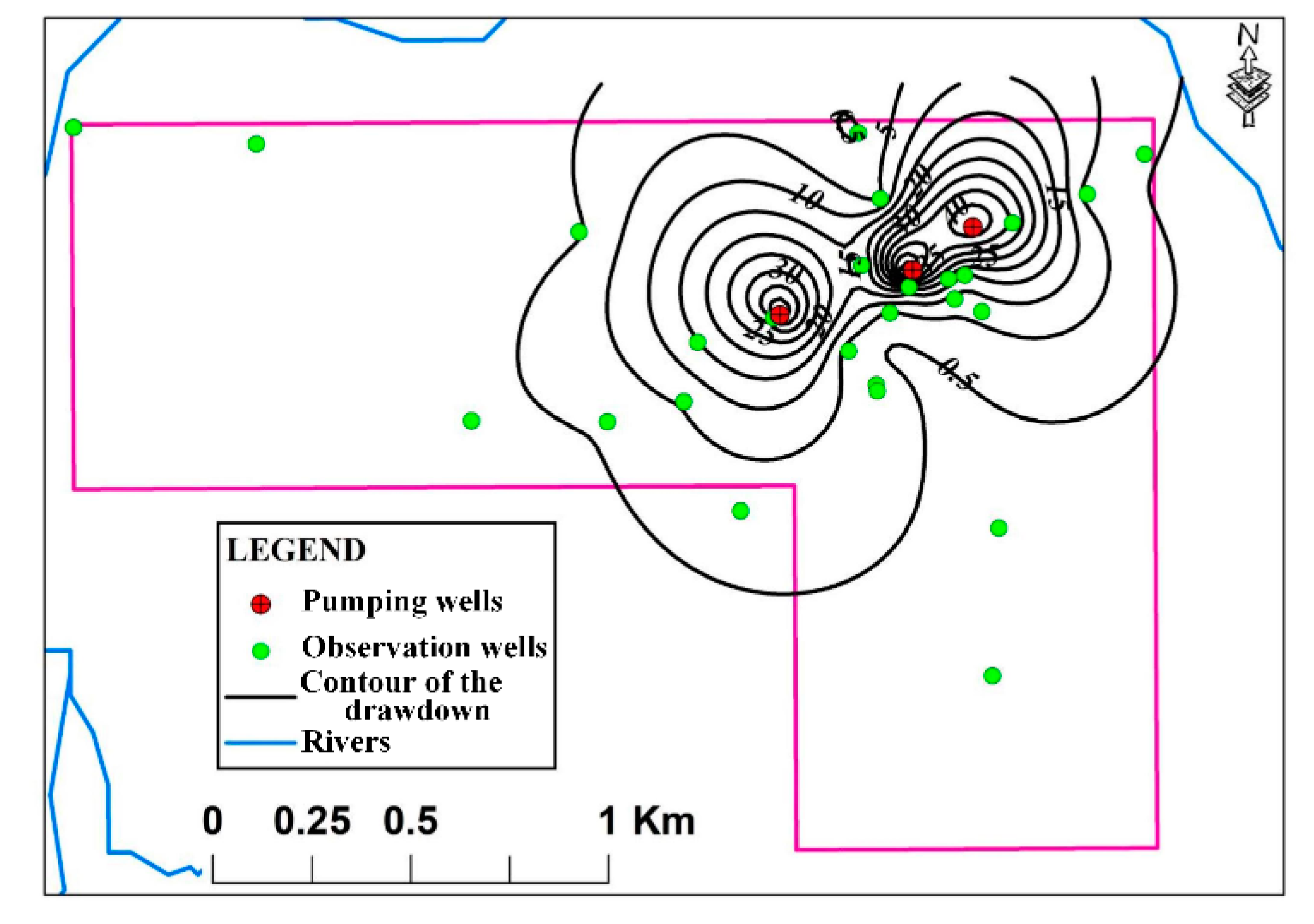
Although the multilayered observation wells are not at the same depths as the boreholes, the contour map of maximum drawdowns for all wells is firstly projected in the same plain. From Figure 3, the distribution of maximum drawdown is highly uniform. The long axis of the maximum drawdown is approximately 45° northeast, and the length of the influence is approximately 1.50 km. The short axis of maximum drawdown is approximately 45° northwest, and the length of the influence is approximately 1.0 km.

3.2. Relationship of Water Levels between Observation and Pumping Wells

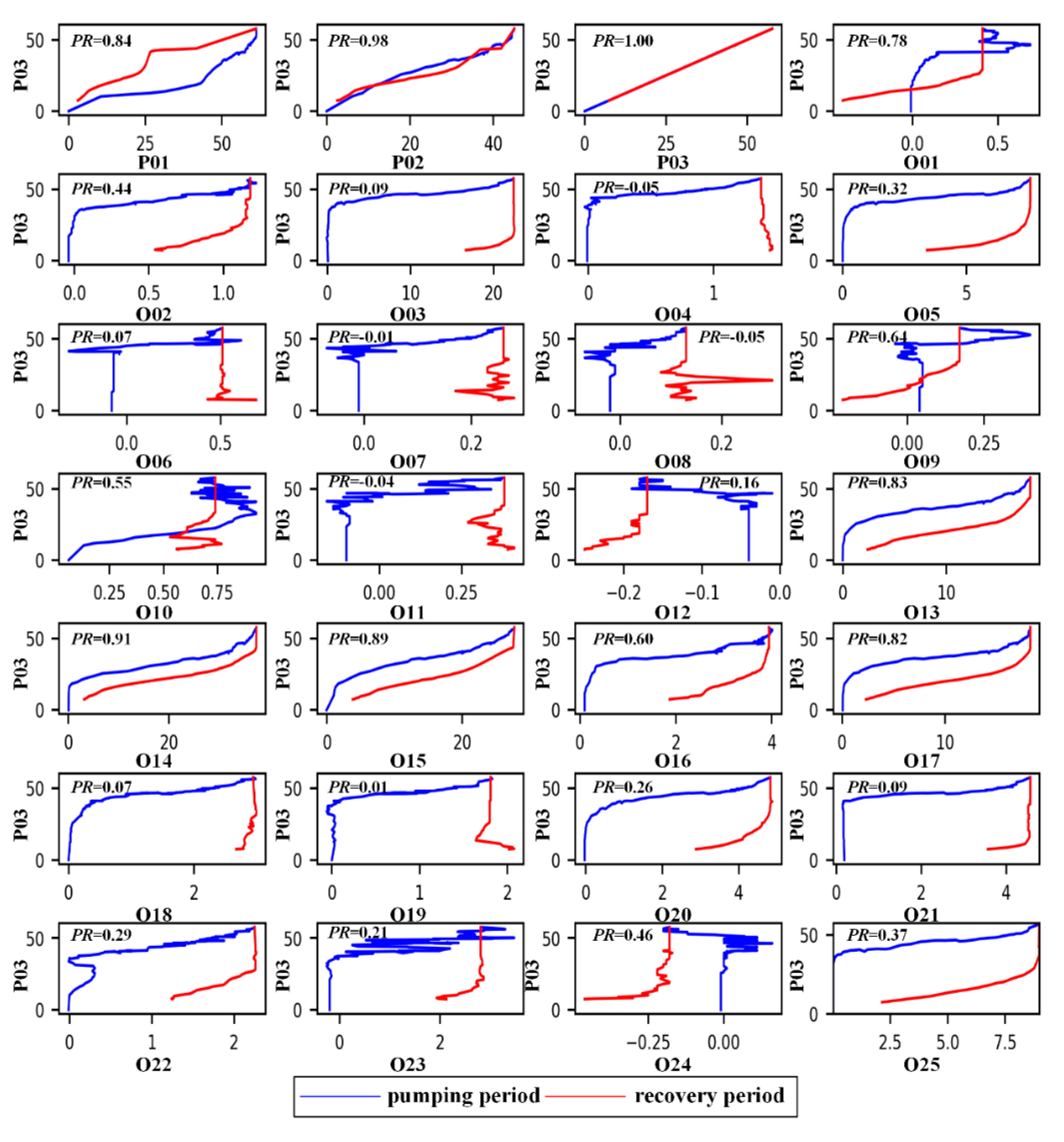
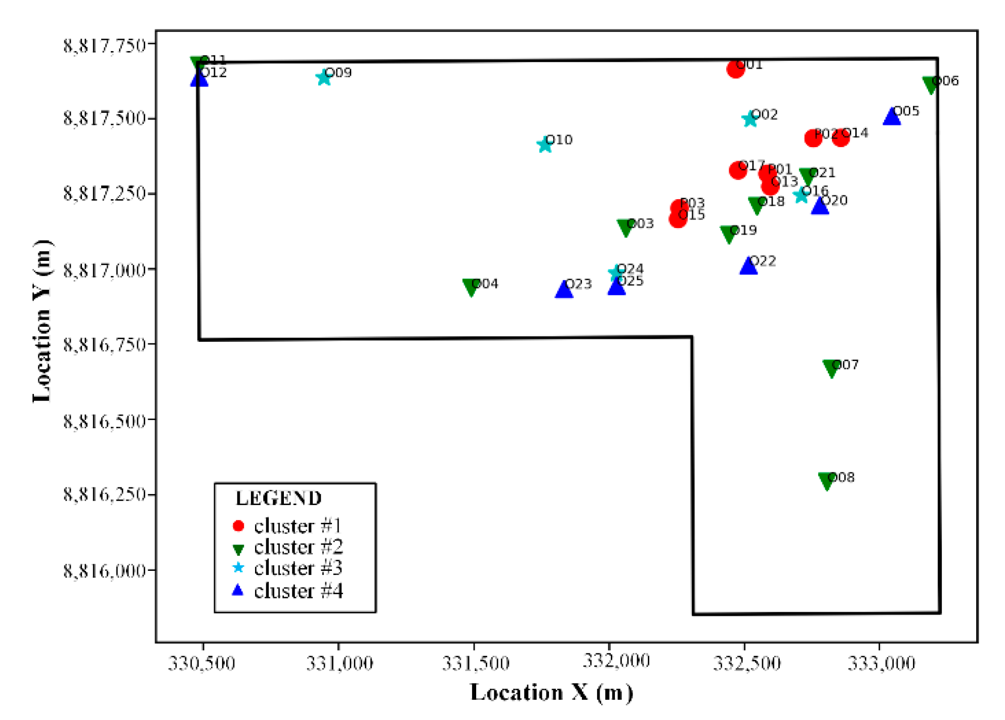
Pumping well P03 is located almost at the center of the study area, with considerable pumping rates, and was thus chosen as a representative pumping well to demonstrate relationships with other wells. The relationship over the pumping period (blue line) and the restoring period (red line) between well P03 and other wells are shown in Figure 4. K-means clustering of the Pearson correlation coefficient (PR) for 28 observation wells (Figure 5) is drawn to clarify the relationship. Four clusters (clusters #1, #2, #3, and #4) are divided based on the value of the Pearson correlation coefficient. The first cluster (cluster #1) includes observation wells P01, P02, P03, O13, O14, O15, O17, and O01, which have the higher PR (over 0.75) with pumping well P03. The second cluster (cluster #2) consists of wells O03, O18, O19, O21, O04, O06, O11, O07, and O08, with the correlation ranging from 0.44 to 0.64. The PR in the third cluster (cluster #3) for observation wells O02, O10, O16, O24, and O09 varied from 0.16 to 0.32. Observation wells O23, O25, O22, O20, O05, and O12 are attributed to the fourth cluster (cluster #4), with a PR less than 0.10. Observation wells with higher PR values basically surrounded the three pumping wells. It should be noticed that observation wells with relatively higher PR values (cluster #2) did not always surround three pumping wells. For example, wells O11 and O08 are a little farther away from the pumping wells; observation wells for cluster #3 and #4 are progressively farther away from the pumping wells. The high PR value suggests that the hydraulic connections for the wells in cluster #1 are perfect.

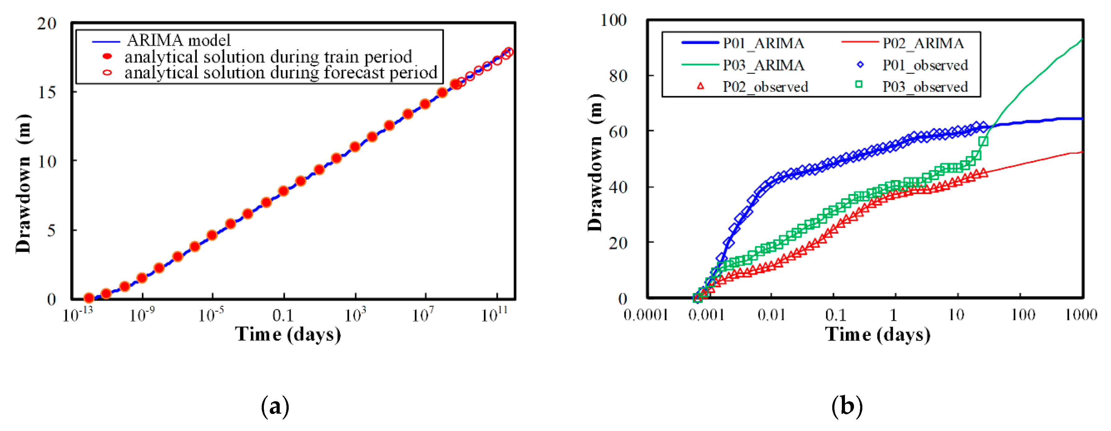
3.3. Predictions of Drawdowns within Pumping Wells

Drawdowns within pumping wells are direct responses of groundwater pumping. Under the condition of a constant pumping rate, drawdowns within wells will be progressively increased. The ARIMA method is used to predict the change of the drawdown. For validating the accuracy of the ARIMA model, a hypothetical confined aquifer satisfying the Theis model is first established. Any parameters in the Theis model can be assumed. Pumping rate, the thickness of the aquifer, hydraulic conductivities, storativities, and the radial distance away from the pumping well in the Theis model for an observation well is set as 100.00 m³/d, 20.00 m, 0.50 m/d, 10⁻⁶ m⁻¹, and 5.00 m, respectively. The relative error, defined as the ratio of the absolute error between the simulated and analytical drawdowns to the analytical solutions, was only 0.86% after about 1.37 × 10⁹ years of pumping for the hypothetical Theis model (Figure 6a), suggesting that the ARIMA method can be used to accurately predict changes of the drawdown with time. After making the time series stationary and training the ARIMA model with a p-value less than 10⁻³, changes of the drawdown in three pumping wells P01, P02, and P03 could be obtained (Figure 6b). After 1000 days, the predicted maximum drawdown in wells P01, P02, and P03 after 3 years was 64.53 m, 52.50 m, and 92.88 m, respectively. It should be noticed that the observed drawdowns in well P03 had an abrupt increase from 51.00 m to 56.00 m during the period from about 20 days to 25 days, which may be caused by the assumption of a linear aquifer system in the ARMA model [26,27]; thus, the predicted drawdown also shows an obvious increasing trend.

3.4. Predictions of Drawdowns in Observation Wells

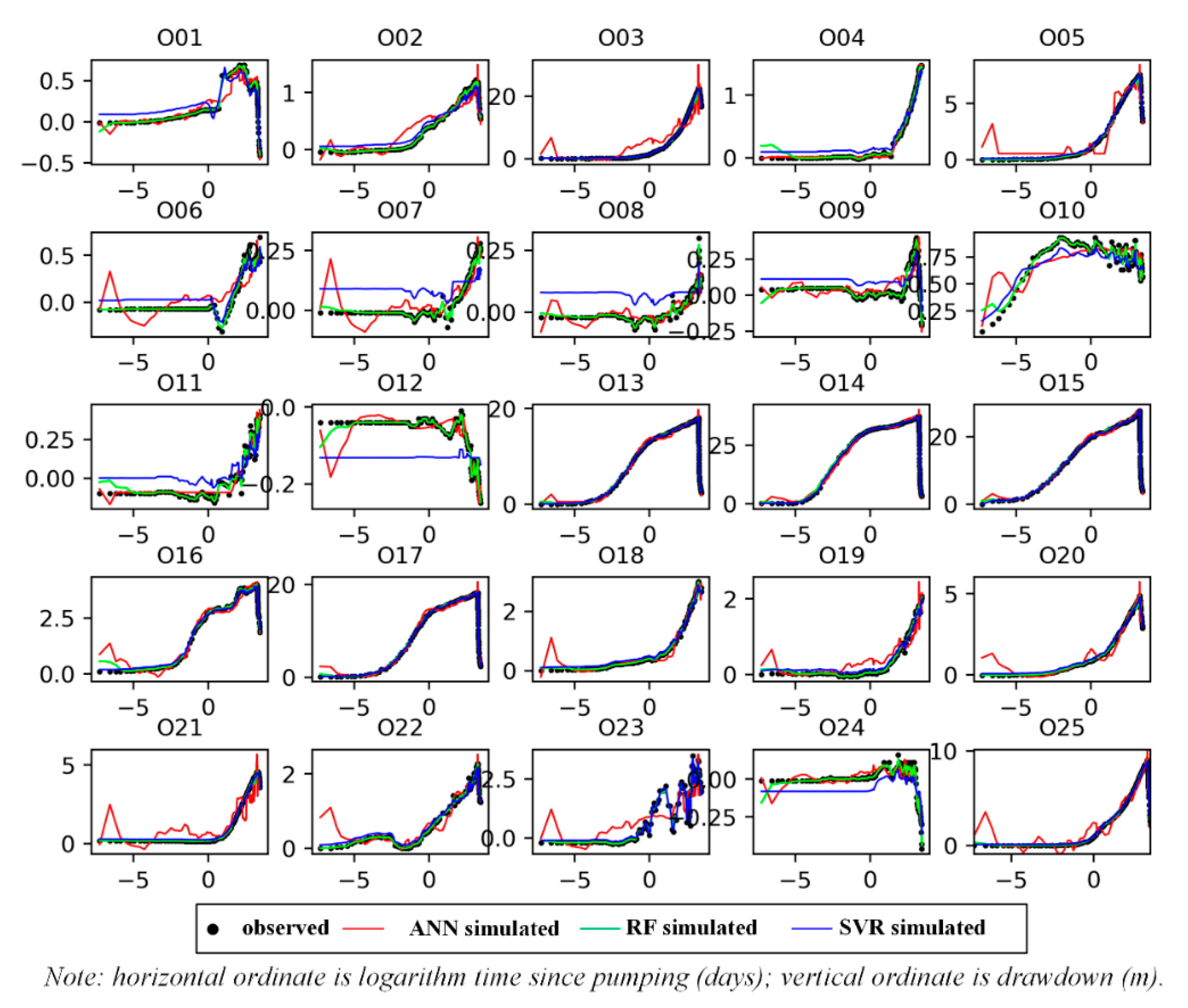
The pumping tests here were carried out in the period from the dry season to the wet season. As a result, changes of the drawdown in observation wells were mainly subject to the combined influences of precipitation conditions, the pumping rate of three wells, and aquifer properties. Independent variables include the precipitation and the drawdown in three pumping wells. The dependent variable is the drawdown for each observation well. The ANN, RF, and SVR methods were all applied to predict the drawdowns for 25 observation wells. Both the first and second hidden layer of the ANN model were set as 10, the number of trees in the RF method was set at 500, the radial basis function (rbf) was used as the kernel function of the SVR model, and the regularization parameter c was set as 10,000. Changes in simulated drawdowns over time from ANN, RF, and SVR methods are shown in Figure 7. All three methods can simulate the trend of groundwater level changes well. The average RMSE value for the 25 observation wells for the ANN, RF, and SVR methods is 0.51 m, 0.13 m, and 0.13 m, respectively, suggesting that the RF and SVR methods show relatively better results than the ANN method. Li et al. [28] applied RF, ANN, and SVM to forecast lake water level variations, and also found the RF model exhibits the best performance, which is consist with the findings in this study.

4. Discussion

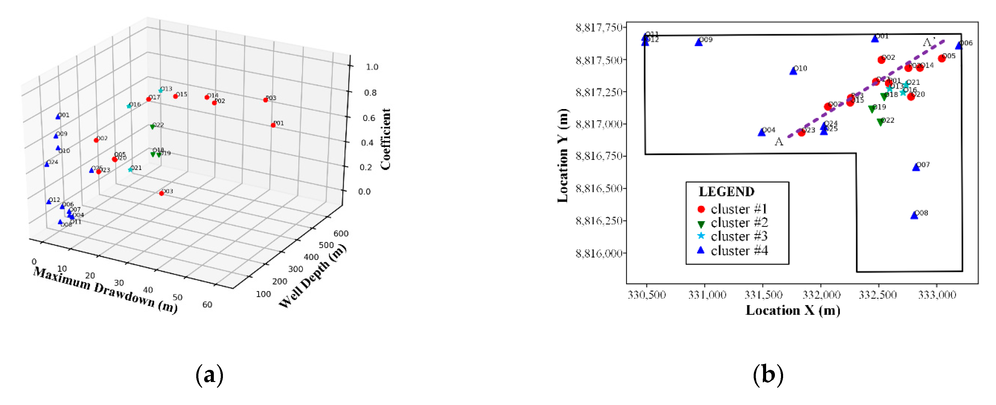
As discussed earlier, the PR coefficient only demonstrates the relationship of groundwater level changes for two wells. The k-means cluster using three variables (PR coefficient, drawdown, and well depth) is further divided to find the hydraulic connections between these wells. It can be clearly observed from Figure 8a that cluster #1 (wells P01, P02, P03, O02, O03, O05, O14, O15, O17, O20, and O23) is located at a depth ranging from 250 m to 350 m, suggesting the hydraulic connection are perfect at such a depth. The clustering was projected to a two-dimensional (2D) map (Figure 8b), and it was found that the axis of maximum drawdown was along the line AA’ from the southwest to the northeast. Furthermore, the drawdown south of line AA’ is better than that north of the line, which is importantly caused by the fact that the existing syncline, which makes an aquifer with perfect permeability, extends from the northwest to the southeast (Figure 1b), and thus the permeability at the southeastern part is better than that in the northwest.

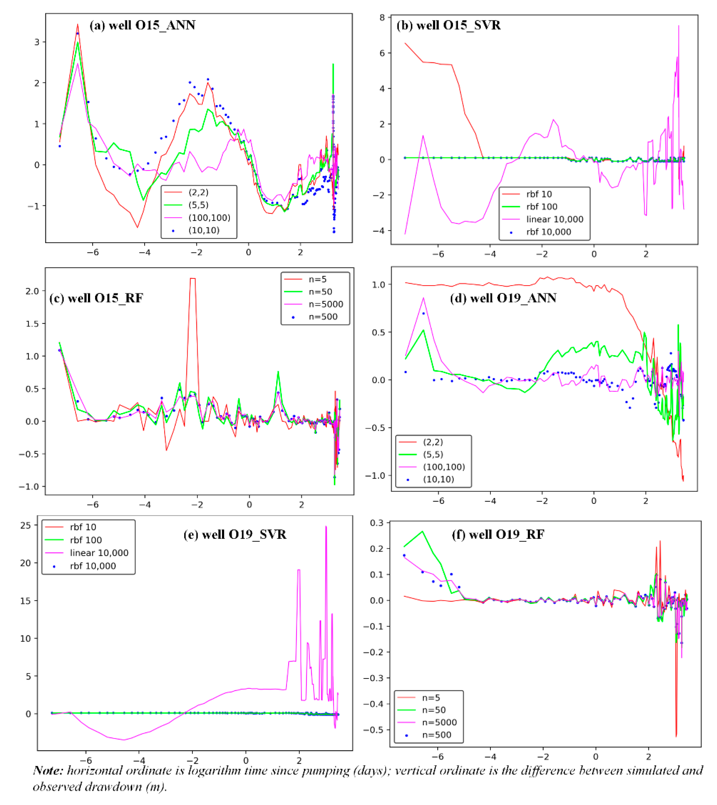
Established ANN, SVR, and RF models can accurately predict the change of the drawdown for 25 observation wells; however, the parameters in these models may have certain influences on the model results. Well O15 with big drawdowns (cluster #1) and well O19 with small drawdowns (cluster #2) were selected to evaluate the influences of parameters on model results.

Table 3. List of root mean square error (RMSE) values and average relative error in ANN, SVR, and RF methods for wells O15 and O19.

Models	Parameters		RMSE (m)		Average Relative Error (%)
			Well O15	Well O19	Well O15	Well O19
ANN Model	number of the first and the second hidden layers	(2, 2)	5.1972	0.3516	90.64	220.01
		(5, 5)	0.8717	0.1834	9.66	195.83
		(10, 10)	0.5844	0.1998	16.30	84.34
		(100, 100)	0.5085	0.1237	10.56	89.60
SVR Model	kernel function (the radial basis function (rbf) and linear) and parameter c	rbf, c = 10	1.1462	0.0941	76.40	96.87
		rbf, c = 100	0.0926	0.0941	1.90	96.87
		rbf, c = 1000	0.0926	0.0941	1.90	96.87
		linear, c = 1000	2.6271	5.4130	58.95	2443.24
RF Model	number of trees (n)	n = 5	0.2429	0.0551	14.13	22.01
		n = 50	0.2071	0.0468	11.57	13.38
		n = 500	0.1842	0.0416	11.17	14.84
		n = 5000	0.1853	0.0394	10.91	15.17

lists the value of parameters, RMSE, and average relative errors in the three models for wells O15 and O19. The relative error here is defined as the average ratio of absolute error between simulated and observed drawdown to the observed drawdown for all observed results.

Figure 9 reveals the influences of model parameters on model bias, which is the difference between the simulated and the observed drawdown. For the ANN model, with the increase of the hidden layers, the model bias will be gradually reduced, and when the number of the first and second hidden layers is over 5, RMSE is less than 0.88 m and 0.20 m for wells O15 and O19, respectively, but the average relative errors for well O15 and O19 are about 15% and 85%, respectively. For the SVR model, results using the rbf kernel function give better predictions than those using the linear kernel function, and the higher value of parameter c will improve the accuracy of the models. However, when the value of c is greater than 100, the models with the rbf kernel function results are not improved significantly for wells O15 and O19, with RMSEs over 0.53 m (average relative error about 1.90%) and 1.08 m (average relative error about 96.87%), respectively. Meanwhile, the change of the drawdown for well O19 was less sensitive to the parameter c than that for well O15. The sensitivities to parameters in the RF model for both well O15 and well O19 were less than those from the ANN and SVR models: RMSE values were about 0.18–0.25 m, with a relative error about 11.00–14.00% for well O15, and 0.039–0.055 m, with average relative error about 13.38–22.01% for well O19. Considering RMSE and average relative error, the RF model gives the most accurate results and has fewer sensitivities to parameters; thus, is the most appropriate model in this study.

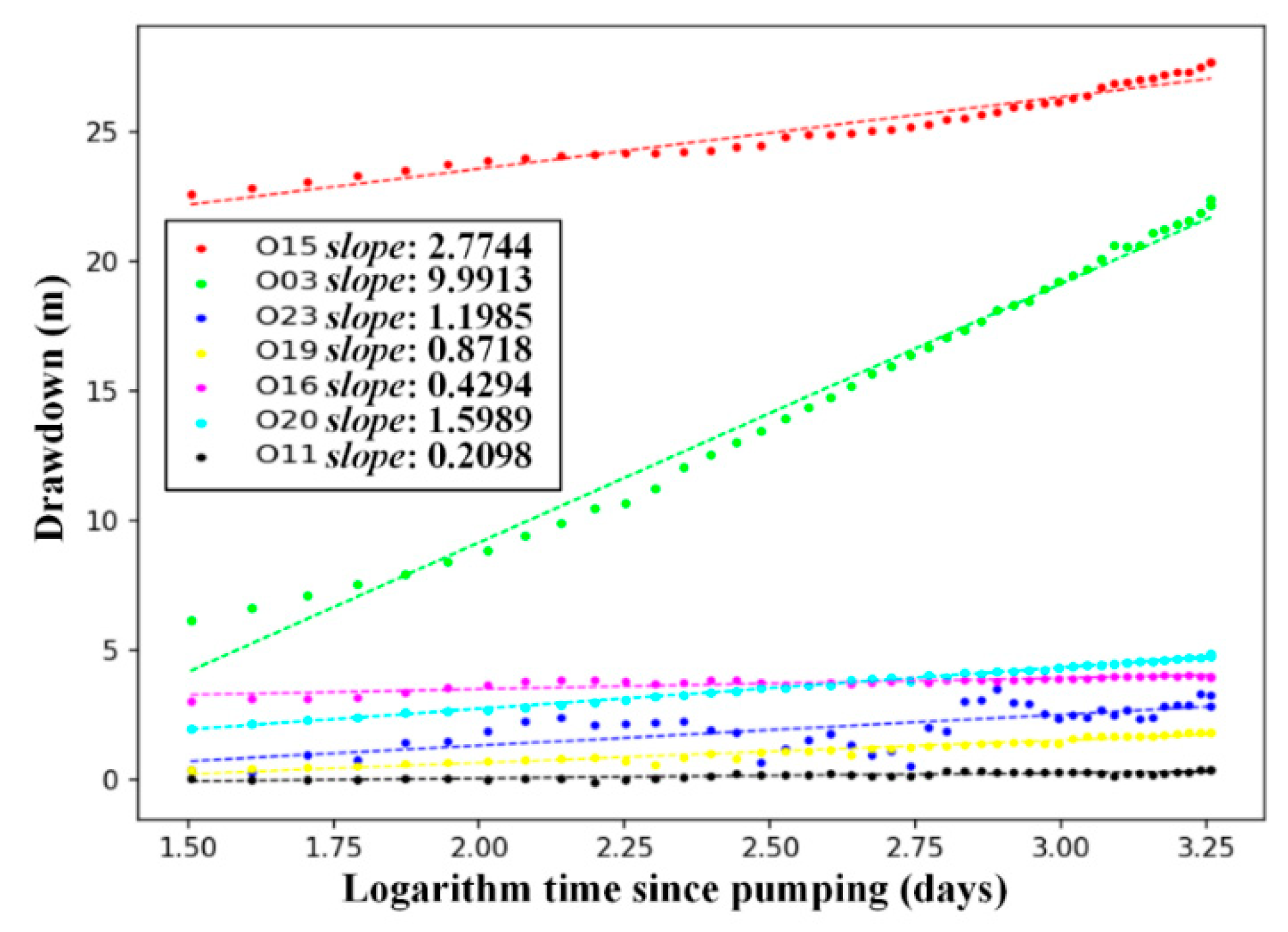
One of the important objectives of pumping tests is to estimate aquifer properties. ML methods lack the mechanics of groundwater flow, and cannot directly estimate hydraulic conductivity like analytical solutions. From the Theis model, the relationship between the drawdown and the logarithm time since the start of pumping become linear when time is long enough and the model satisfies the assumption of a Theis model. Therefore, wells O15, O03, O23, O19, O16, O20, and O11, which had relatively higher PR coefficients with the pumping rates, were chosen to establish the linear regressive model (Figure 10). The slope of the linear regressive model has a negative relationship with the value of the hydraulic conductivity, and thus can be used to estimate the hydraulic conductivity like the Theis model. Well O03 had the highest slope (almost 10), and estimated average hydraulic conductivity from well P03 to O03 was about 0.15 m/d, given that the pumping rate was about 2800 m³/d and the average aquifer thickness was about 330 m. It was noticed that well O11 had the lowest slope (about 0.21) and was the furthest distance away from the pumping wells among these wells; in addition, the estimated hydraulic conductivity may have reached about 7.00 m/d if the average aquifer thickness was set as 350 m. The estimated average hydraulic conductivity for wells O13, O23, O19, O16, and O20 was about 1.23 m/d, which is at the same magnitude as in previous studies (0.65 m/d) on this region.

5. Conclusions

Pumping tests are very important means for investigating aquifer properties; however, common analytical solutions become invalid for interpreting the data when aquifers are anisotropic and heterogeneous. The paper explored the potential of ML methods for analyzing pumping test information in a field site. The study area is located at a mine area that has a pumping test with three pumping wells and 28 observation wells, over the period of about 32 days. Results found that ML methods can be successfully applied to simulate groundwater level changes induced by pumping and retrieve the relationship of groundwater levels between wells. Improving our understanding of pumping tests using ML methods requires (1) providing the fast and visual pictures of drawdowns between pumping wells and observation wells; (2) forecasting the changes of drawdowns in the observation wells, as well as in the pumping wells; (3) inferring the possible pathways of hydraulic connections in complex geology formations; (4) estimating average hydraulic conductivities. The main conclusions include:

(1)

Rather than the mere contour map of the maximum drawdowns, the relationships of the drawdown over the period of pumping tests between wells provide a visual picture using ML methods, and the cluster of Pearson correlation coefficient shows the hydraulic connections between wells;

(2)

The ARIMA method can be used to effectively predict the time-series changes of drawdowns in three pumping wells. In the hypothetical Theis model, the relative error of drawdowns is only 0.86% after 1.37 × 109 years. The predicted maximum drawdown in well P01, P02, and P03 after 3 years is 64.53 m, 52.50 m, and 92.88 m, respectively;

(3)

Trained ANN, SVR, and RF models can reasonably capture the change of drawdowns in 25 observation wells induced by pumping; however, SVR and RF models provide better estimates, with average RMSE values for drawdowns of 0.13 m;

(4)

K-means clustering using the Pearson correlation coefficient, the maximum drawdown, and well depth visually shows a preferable pathway, with the good permeability under depths ranging from 250 m to 350 m;

(5)

Model parameters have certain influences on the simulated drawdowns for ANN, SVR, and RF models, but the RF model shows the least sensitivity to the value of the parameters, and has the best performance when compared with observed results;

(6)

With the assumption of the Theis model, the linear regressive method may be used to roughly estimate the value of hydraulic conductivity, and the results in this paper are consistent with the previous studies.

The radius of influence (ROI) [29] in pumping tests is not discussed in this paper, but will be in future work when considering the combined influences of groundwater level and groundwater quality.

References

- Nace, R.L. (Ed.) Scientific Framework of World Water Balance; UNESCO Technical Papers in Hydrology; UNESCO: Paris, France, 1971; pp. 7–27. [Google Scholar]
- Fetter, C.W. Applied Hydrogeology, 4th ed.; Prentice-Hall, Inc.: Upper Saddle River, NJ, USA, 2001. [Google Scholar]
- Rajaee, T.; Ebrahimi, H.; Nourani, V. A review of the artificial intelligence methods in groundwater level modeling. J. Hydrol. 2019, 572, 336–351. [Google Scholar] [CrossRef]
- Yoon, H.; Jun, S.C.; Hyun, Y.; Bae, G.O.; Lee, K.K. A comparative study of artificial neural networks and support vector machines for predicting groundwater levels in a coastal aquifer. J. Hydrol. 2011, 396, 128–138. [Google Scholar] [CrossRef]
- Emamgholizadeh, S.; Moslemi, K.; Karami, G. Prediction the groundwater level of bastam plain (Iran) by artificial neural network (ANN) and adaptive neuro-fuzzy inference system (ANFIS). Water Resour. Manag. 2014, 28, 5433–5446. [Google Scholar] [CrossRef]
- Ebrahimi, H.; Rajaee, T. Simulation of groundwater level variations using wavelet combined with neural network, linear regression and support vector machine. Glob. Planet. Chang. 2017, 148, 181–191. [Google Scholar] [CrossRef]
- Lee, S.H.; Lee, K.K.; Yoon, H. Using artificial neural network models for groundwater level forecasting and assessment of the relative impacts of influencing factors. Hydrogeol. J. 2019, 27, 567–579. [Google Scholar] [CrossRef]
- Xu, T.F.; Valocchi, A.J.; Choi, J.; Amir, E. Use of machine learning methods to reduce predictive error of groundwater models. Groundwater 2014, 52, 448–460. [Google Scholar] [CrossRef]
- Xu, T.F.; Valocchi, A.J. Data-driven methods to improve baseflow prediction of a regional groundwater model. Comput. Geosci. 2015, 85, 124–136. [Google Scholar] [CrossRef] [Green Version]
- Sameen, M.I.; Pradhan, B.; Lee, S. Self-learning random forests model for mapping groundwater yield in data-scarce areas. Nat. Resour. Res. 2019, 28. [Google Scholar] [CrossRef]
- Sun, A.Y.; Scanlon, B.R.; Zhang, Z.Z.; Walling, D.; Bhanja, S.N.; Mukherjee, A.; Zhong, Z. Combining physically based modeling and deep learning for fusing GRACE satellite data: Can we learn from mismatch? Water Resour. Res. 2019, 55, 1179–1195. [Google Scholar] [CrossRef] [Green Version]
- Safavi, H.R.; Esmikhani, M. Conjunctive use of surface water and groundwater: Application of support vector machines (SVMs) and genetic algorithms. Water Resour. Manag. 2013, 27, 2623–2644. [Google Scholar] [CrossRef]
- Gaur, S.; Dave, A.; Gupta, A.; Ohri, A.; Graillot, D.; Dwivedi, S.B. Application of artificial neural networks for identifying optimal groundwater pumping and piping network layout. Water Resour. Manag. 2018, 32, 5067–5079. [Google Scholar] [CrossRef]
- Seyoum, W.M.; Kwon, D.J.; Milewski, A.M. Downscaling GRACE TWSA data into high-resolution groundwater level anomaly using machine learning-based models in a glacial aquifer system. Remote Sens. 2019, 11, 824. [Google Scholar] [CrossRef] [Green Version]
- Lal, A.; Datta, B. Development and implementation of support vector machine regression surrogate models for predicting groundwater pumping-induced saltwater intrusion into coastal aquifers. Water Resour. Manag. 2018, 32, 2405–2419. [Google Scholar] [CrossRef]
- Sajehi-Hosseini, F.; Malekian, A.; Choubin, B.; Rahmati, O.; Cipullo, S.; Coulon, F.; Pradhan, B. A novel machine learning-based approach for the risk assessment of nitrate groundwater contamination. Sci. Total Environ. 2018, 644, 954–962. [Google Scholar] [CrossRef] [Green Version]
- Granda, J.M.; Donina, L.; Dragone, V.; Long, D.L.; Cronin, L. Controlling an organic synthesis robot with machine learning to search for new reactivity. Letter 2018, 559, 377–381. [Google Scholar] [CrossRef]
- Nwachukwu, A.; Jeong, H.; Pyrcz, M.; Lake, L.W. Fast evaluation of well placements in heterogeneous reservoir models using machine learning. J. Pet. Sci. Eng. 2018, 163, 463–475. [Google Scholar] [CrossRef]
- Mendelsohn, F. The Geology of the North Rhodesian Copperbelt; Macdonald: London, UK, 1961; pp. 351–405. [Google Scholar]
- François, A. L’extremité Occidentale Del’arc Cuprifère Shabien Etude Geologique; Bureau D’études Géologiques; Aulhenlie Investment Consulting (China) Lo. Ltd. Translation in 2006; Gécamines-Exploitation: Likasi, Zaïre, 1973. (In Chinese) [Google Scholar]
- Takafuji, E.H.M.; Rocha, M.M.; Manzione, R.L. Groundwater level prediction/forecasting and assessment of uncertainty using SGS and ARIMA models: A case study in the Bauru Aquifer System (Brazil). Nat. Resour. Res. 2019, 28. [Google Scholar] [CrossRef] [Green Version]
- Zhang, M.L.; Hu, L.T.; Yao, L.L.; Yin, W.J. Surrogate models for sub-region groundwater management in the Beijing plain, China. Water 2017, 9, 766. [Google Scholar] [CrossRef] [Green Version]
- Tyralis, H.; Papacharalampous, G.; Langousis, A. A brief review of Random Forests for water scientists and practitioners and their recent history in water resources. Water 2019, 11, 910. [Google Scholar] [CrossRef] [Green Version]
- Pedregosa, F.; Varoquaux, G.; Gramfort, A.; Michel, V.; Thirion, B.; Grisel, O.; Blondel, M.; Prettenhofer, P.; Weiss, R.; Dubourg, V.; et al. Scikit-learn: Machine learning in Python. J. Mach. Learn. Res. 2011, 12, 2825–2830. [Google Scholar] [CrossRef]
- Haroon, D. Python Machine Learning Case Studies: Five Case Studies for the Data Scientist; Apress: New York, NY, USA, 2017; Volume 1. [Google Scholar]
- Yihdego, Y.; Danis, C.; Paffard, A. Why is the groundwater level rising? A case study using HARTT to simulate groundwater level dynamics. J. Water Environ. Res. 2017, 89, 2142–2152. [Google Scholar] [CrossRef] [PubMed]
- Yihdego, Y.; Webb, J.A. Modeling of bore hydrograph to determine the impact of climate and land use change in a temperate subhumid region of south-eastern Australia. Hydrogeol. J. 2011, 19, 877–887. [Google Scholar] [CrossRef]
- Li, B.; Yang, G.S.; Wan, R.R.; Dai, X.; Zhang, Y.H. Comparison of random forests and other statistical methods for the prediction of lake water level: A case study of the Poyang Lake in China. Hydrol. Res. 2016, 47, 69–83. [Google Scholar] [CrossRef] [Green Version]
- Yihdego, Y. Engineering and enviro-management value of radius of influence estimate from mining excavation. J. Appl. Water Eng. Res. 2018, 6, 329–337. [Google Scholar] [CrossRef]
Figure 1.
Location of the study area: (a) the geology and location of wells in the plain; (b) the geology along the cross-section line LL.
Figure 2.
Change of precipitation over the entire pumping test.
Figure 3.
Contour map of maximum drawdown in the Musonoi mine area.
Figure 4.
Plot of drawdown relationship between well P03 and 28 observation wells over the entire period of pumping.
Figure 5.
Distribution and k-means clustering of the Pearson correlation coefficient for 28 wells.
Figure 6.
Train and forecast of drawdowns within pumping wells, (a) the Theis model; (b) the autoregressive integrated moving average (ARIMA) model.
Figure 7.
Changes of the simulated drawdowns with time from artificial neural network (ANN), random forest (RF), and support vector machine (SVR) methods for 25 observation wells.
Figure 8.
Schematic figures of the k-means clustering demonstrated in three-dimensional (3D) and two-dimensional (2D) space using the PR coefficient, drawdown, and well depth. (a) 3D space, (b) 2D space.
Figure 9.
Influence of parameters in ANN, SVR, and RF models on the simulated drawdowns for wells O15 and O19: (a–c) represent the results from ANN, SVR, and RF methods for well O15, respectively; (d–f) represent the results from ANN, SVR, and RF methods for well O19, respectively.
Figure 10.
Relationship of drawdowns and time for wells O15, O03, O23, O19, O16, O20, and O11.