Improved Landsat-Based Water and Snow Indices for Extracting Lake and Snow Cover/Glacier in the Tibetan Plateau


1
Key Laboratory of Tibetan Environmental Changes and Land Surface Processes, Institute of Tibetan Plateau Research, Chinese Academy of Sciences, Beijing 100101, China
2
Institute of Geographic Sciences and Natural Resources Research, Chinese Academy of Sciences, Beijing 100101, China
3
University of Chinese Academy of Sciences, Beijing 100101, China
4
Shaanxi Key Laboratory of Earth Surface System and Environmental Carrying Capacity, Northwest University, Xi’an 710727, China
*
Author to whom correspondence should be addressed.
Water 2020, 12(5), 1339; https://doi.org/10.3390/w12051339
Submission received: 22 February 2020
/
Revised: 20 April 2020
/
Accepted: 26 April 2020
/
Published: 8 May 2020
(This article belongs to the Special Issue Applications of Remote Sensing and GIS in Hydrology II)
Abstract
:Identifying water and snow cover/glaciers (SCG) accurately is of great importance for monitoring different water resources in the Tibetan Plateau. However, discriminating between water and SCG remains a difficult task because of their similar spectral characteristic according to the physical principles of remote sensing. To efficiently distinguish different kinds of water resources automatically, here we proposed two new indices including: (i) the normalized difference water index with no SCG information (NDWIns) to extract lake water and suppress SCG: and (ii) the normalized difference snow index with no water information (NDSInw) to extract SCG and suppress lake water. Both new water and snow indices were tested in the Tibetan Plateau using Landsat series, showing that the overall accuracies of NDWIns and NDSInw were in the range of 94.6–97.0% and 94.9–97.0% in mapping the lake water from SCG and mapping the SCG from lake water, respectively. Further comparisons suggest that these new two indices improved upon the previous normalized difference snow index/modified normalized difference water index (NDSI/MNDWI) in mapping the water body and SCG. While the present study only focuses on the validation over certain areas in Tibetan Plateau, the newly proposed NDWIns and NDSInw have the potential for better monitoring the lake water and snow/glacier areas over other cold regions around the globe.
1. Introduction
As key components of the water cycle, lakes and snow cover/glaciers (SCG) are vital indicators of climate change [1]. Lakes and SCG also play an important role in the prevention of water scarcity and world sustainable development [2]. Therefore, understanding the changes in quantity and areal extent of lakes and glaciers is necessary to assess regional and global water resources [3].
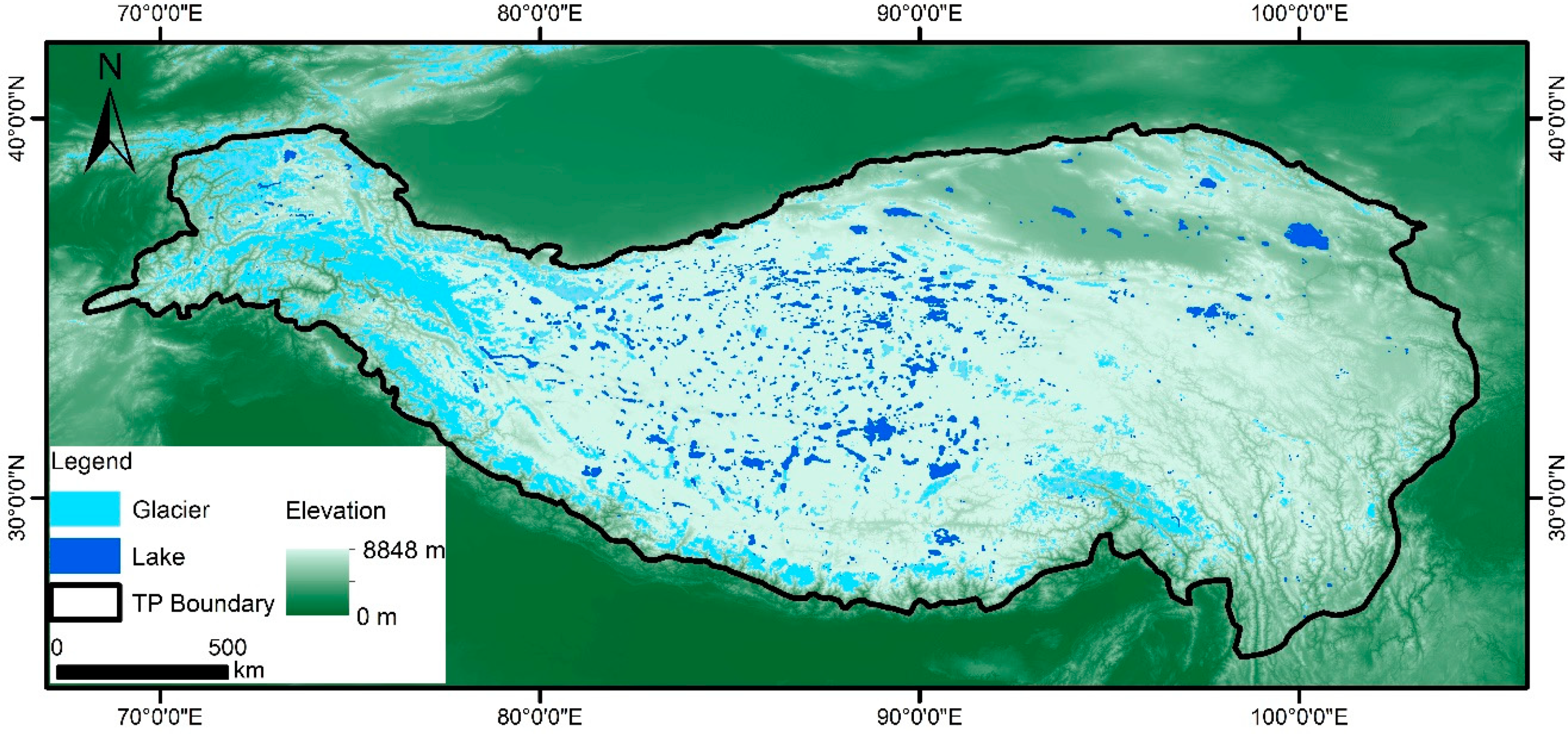
With an average altitude over 4000 m, the Tibetan Plateau (TP), also known as the “Asian Water Tower” [4] and the “Third Pole” [5,6], is the headwater of more than ten large rivers in Asia. Because of the cold climate, there are 36,800 glaciers on the TP (Figure 1), covering an area of 49,873 km2 (~2% of the total plateau’s area), distributed over the major mountain ranges [7]. Glaciers in the TP were found to be decreasing according to the reduction of glacier length and area since the 1970s [7] due mainly to the recent rapid temperature increase [6,8]. In addition, with more than one thousand lakes having a total free-water area of ca. 42,521 km2 (Figure 1), the TP has the most inland lakes in number and area in China and boasts the greatest concentration of high-altitude inland lakes in the world [9,10]. Satellite observations have found that about 81% of the lakes in the TP experienced a trend to increase in area between the 1970s and 2010, and the glacier-fed lakes expanded faster than lakes without glacier supplement [11].
The above mentioned changes in lakes and glaciers have been suggested to be partially caused by the significant warming in the past few decades [6,10]. The warming trend in the TP was found to be significantly higher than the other areas of the world in recent decades [8,12]. The changing climate also made the distribution of land surface water bodies more uneven [13,14,15], because the intensity and frequency of extreme disasters have increased. In this context, the TP is extremely vulnerable to geological disasters such as landslides, debris flows, glacial lake outbursts, and snow and ice disasters [16]. However, only a few observation stations have been established for lake monitoring in the entire TP [9,17]. With the rapid development of remote sensing technology, spatial and temporal distributions of water resources can be monitored from multiple satellites, which are particularly useful and important in remote and inaccessible cold regions with few gauging stations owing to their formidable natural conditions [18]. Therefore, accurately monitoring lakes and snow/glaciers using satellite data is important for not only understanding how the water resources in cold regions response to climate change but also for estimating water storage and changes related to disasters in the Asian Water Tower [6,19].
Numerous studies have been conducted to map water bodies [20] and SCG [21] using optical remote sensing data over the past three decades. Although manual methods and supervised classification usually achieve satisfactory results, both are too time consuming when they are used for long-time series at large scales. Index-based methods provide an alternative approach to achieve this goal more effectively. For example, the normalized difference water index (NDWI), which combines green and near-infrared (NIR) bands, and the snow grain size index (SGI), employing similar bands, are used for mapping water bodies and snow cover respectively [22,23]. Hall et al. (1995) developed the normalized difference snow index (NDSI) to map snow cover using Moderate Resolution Imaging Spectroradiometer (MODIS) data [24]. A decade later, the modified normalized difference water index (MNDWI) employing the same bands was introduced for urban water bodies mapping [25]. Before the normalized difference forest snow index (NDFSI) was proposed to map snow-covered forests as distinguished from snow-free forests [26], it had already been employed to estimate the NDWI for shoreline mapping [27]. Moreover, a combination of the green band and short-wave infrared 2 (SWIR2) band has been applied to map snow cover and water bodies, respectively [28,29]. Additionally, before Rogers and Kearney (2004) suggested mapping water bodies using the red band and short-wave infrared 1 (SWIR1) band [30], it had been developed by Xiao et al. (2001) to detect and monitor SCG in Turkey [31]. Note that previous studies used similar methods to extract inland water bodies and SCG due to the similar reflectance distribution of SCG and water bodies [32], leading to more difficulty in discriminating between surface water bodies and SCG [1].
Several factors. e.g., mountains, snow, clouds, cloud shadows and turbidity are also stumbling blocks in extracting land surface water maps with satellite data [33]. Previous researches have devoted much effort to decrease the noise from cloud surfaces [34,35], vegetation [36], and evergreen coniferous forests [26] in snow cover mapping, and noise from vegetation [37], built-up land [25] and shadow [38] in water mapping. However, little attention has been paid to develop and calibrate water and snow indices in distinguishing water bodies and SCG. Therefore, it is essential to develop an effective new water index to extract water body data from the background that includes SCG, and a new snow index to obtain SCG information from the background that includes water bodies.
To solve the above problem, we aim to develop two new indices according to the minor difference in reflectance between lake water bodies and SCG. To further evaluate the performance of the newly developed water index in mapping lake water bodies from SCG and the snow index in mapping SCG from lake water bodies, a comparison was also made between these two new indices and the previous NDSI/MNDWI. The results presented here will provide a basis for accurately monitoring different kinds of water resources in the Tibetan Plateau.
2. Materials and Methods
2.1. Regional Setting
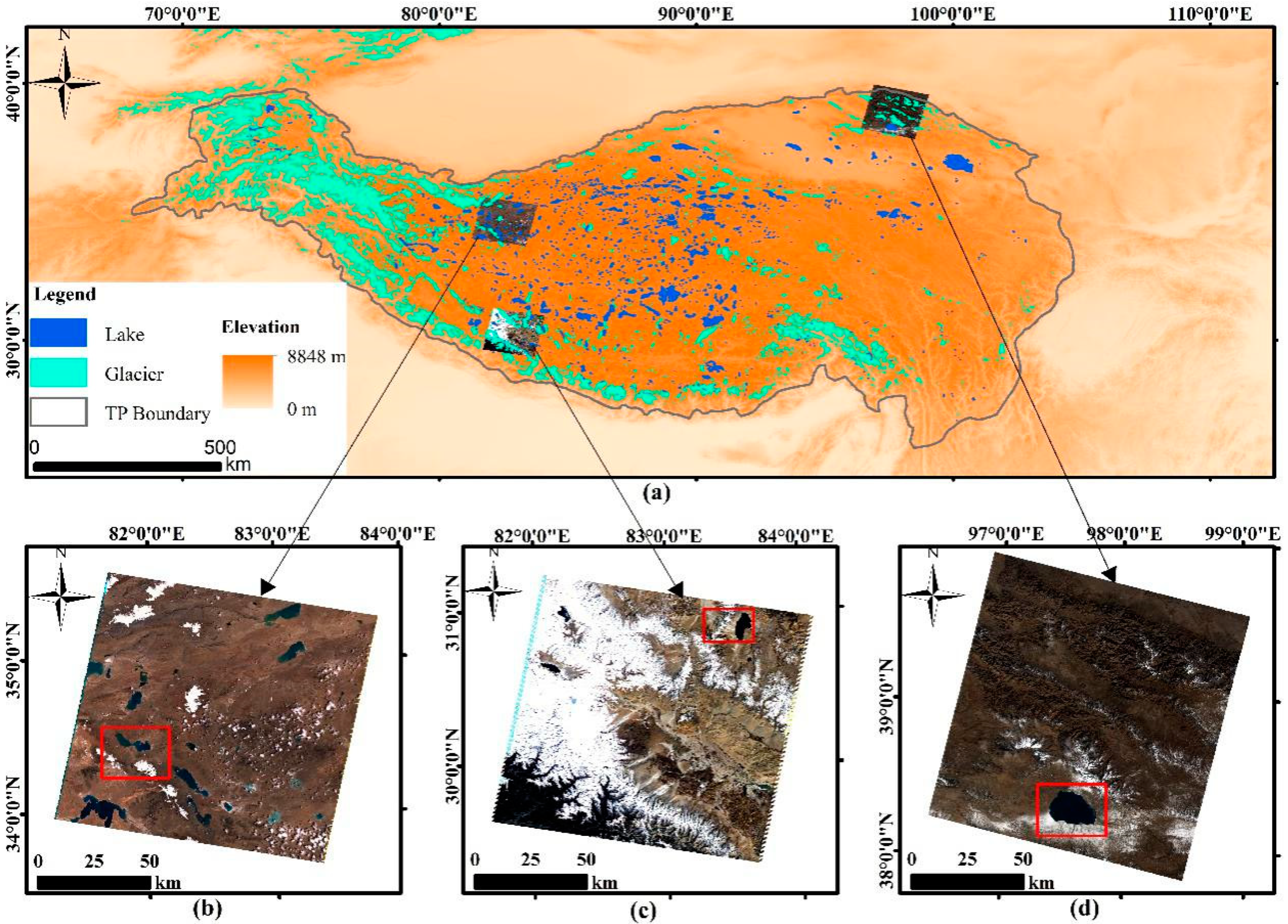
In this study, three regions with different land cover types were selected from the TP to test the performance and robustness of each method (Figure 2). Region I is located in the northeast of the TP and predominantly covered by snow cover and lake water bodies. The average altitude is 4134 m above sea level with flat topography and a total area of 1375 km2. Located in the west of the TP, Region II is characterized by hilly topography, and covered by a glacier, lake water and bare land, with a mean altitude of 4354 m and a total area of 802 km2. Region III is located in the south of the TP with altitudes ranging from 5100 m to 6320 m and a total area of 377 km2. The land cover type in Region III is similar to that in Region II.
2.2. Data
The Landsat imagery captured from Operational Land Imager (OLI), Enhanced Thematic Mapper Plus (ETM+) and Thematic Mapper (TM) has been extensively used in numerous studies in the field of remote sensing over the past three decades (Table 1). It has been widely employed in inland water body and SCG mapping because of its high spatial resolution (http://earthexplorer.usgs.gov). The digital number value in the three Landsat images is corrected to reflectance by the Fast Line-of-Sight Atmospheric Analysis of Spectral Hypercubes (FLAASH) module, which is commonly used in atmospheric correction [29,38,39]. The corresponding high resolution of reference data was acquired from Google Earth.
2.3. Methods
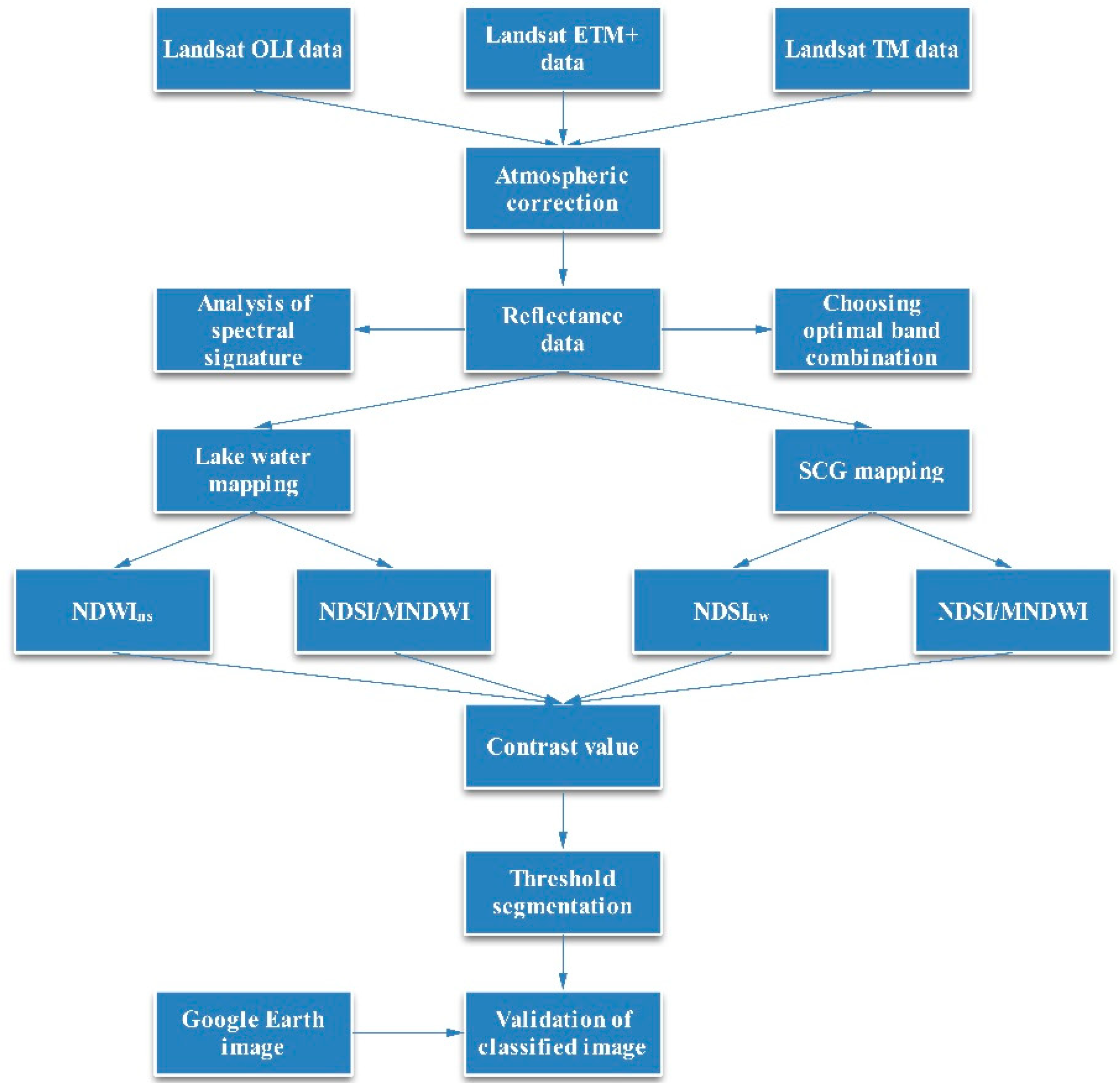
The methodology mainly consists of six procedures: atmospheric correction, analysis of spectral signature, formulation of new indices, calculation of contrast value, image threshold segmentation and validation of classified image. The flowchart of the methodology based on Landsat data in this study is shown in Figure 3.
2.3.1. Spectral Signature of Lake Water and SCG
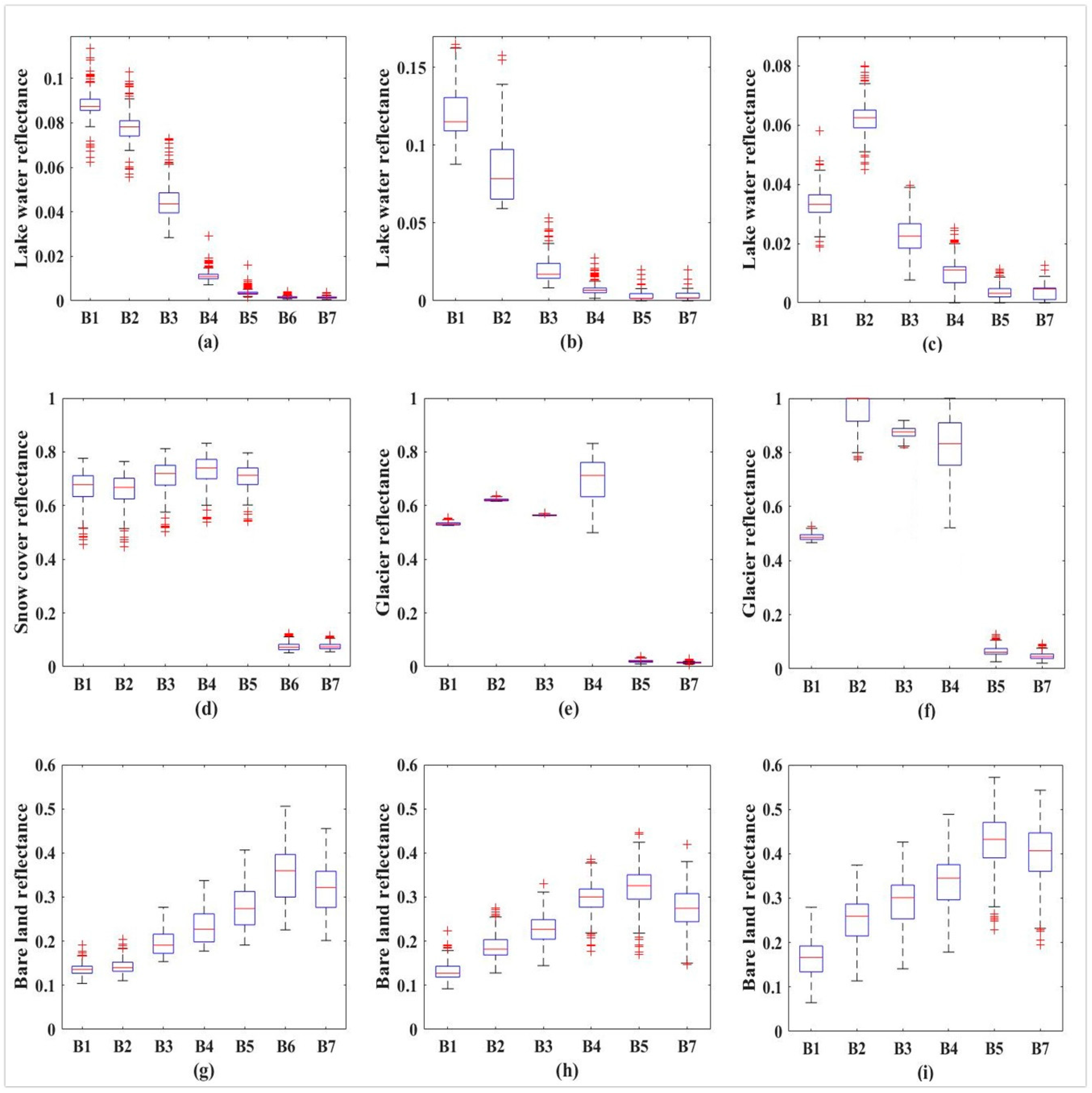
The spectral reflectance distribution of the three land cover types was sampled in each study region based on Landsat multispectral images corrected by the FLAASH model (Figure 4). It is apparent that the reflectance of lake water bodies and SCG shows a declining trend, while the reflectance of bare land exhibits an increasing trend from the visible to infrared bands in general. Previous studies have used this characteristic as an asset to enhance water bodies or SCG information and suppress background information. To distinguish between lake water bodies and SCG, the minor differences in spectral reflectance between lake water bodies and SCG were investigated. It was found that one difference is that the reflectance of lake water bodies decreases from the green band to NIR band steadily, while the reflectance of SCG remains stable or fluctuates slightly from the green band to NIR band. The second difference is that the reflectance of SCG falls sharply, while the reflectance of lake water bodies remains steady or decreases slightly from the NIR band to SWIR1 band.
2.3.2. The Contrast Values of Five Indices between Lake Water and SCG
To discover the optimal band combination in discrimination between lake water bodies and SCG, the contrast values of the extracted image of five common indices [22,23,24,25,28,29,30,31] between lake water bodies and SCG were compared (Table 2). The higher the contrast value, the better the discrimination between lake water bodies and SCG. The contrast value [29] is calculated from the difference between lake water bodies and SCG in each index image in the three study regions using Equation (1).
where CV is the contrast value between foreground and background, Mf is the mean value of foreground, and Mb is the mean value of background.
CV = Mf − Mb
2.3.3. Formulation of Water Index and Snow Index
The formulation of our proposed normalized difference water index with no SCG information (NDWIns) is as follows. The normalized difference between the green band and NIR band remains at a high level in lake water areas, but at a low level in SCG areas (Figure 4). Furthermore, the contrast values between lake water bodies and SCG is great by normalizing the green band and NIR band difference. Considering the reflectance of lake water bodies is negligible and the reflectance of SCG is higher than 0.5 in the NIR band, subtracting double reflectance of the NIR band from the reflectance of the green band maintains the index value of lake water bodies at a high level and decreases the index value of SCG further. Thus, NDWIns is designed to extract water information with noise from SCG:
where ρGreen is the reflectance of the green band, ρNIR is the reflectance of the NIR band. a is an empirical parameter that needs to be calibrated for different study sites. Here we used a value of 2.
NDWIns = (ρGreen − a × ρNIR)/(ρGreen + ρNIR)
The formulation of the normalized difference SCG index with no water information (NDSInw) is as follows. The difference between the NIR band and SWIR1 band remains high in SCG areas and low in lake water areas (Figure 4). Normalizing the NIR band and SWIR1 band difference maintains the index value at a high level in SCG areas and a low value in lake water areas. To further reduce lake water information, a positive value (0.05) is subtracted from the difference value between the NIR band and the SWIR1 band. Thus, the NDSInw is proposed to extract SCG and suppress noise from lake water bodies.
where ρNIR and ρSWIR1 are the reflectance of the NIR band and the SWIR1 band. b is an empirical parameter that needs to be calibrated for different study sites. Here we used a value of 0.05.
NDSInw = (ρNIR − ρSWIR1 − b)/(ρNIR + ρSWIR1)
2.3.4. NDSI and MNDWI
NDSI was proposed by Hall et al. (1995) by normalizing the green band and SWIR1 band difference based on the MODIS data [24]. After a decade, MNDWI [25] also used this band combination to extract different water bodies based on Landsat data. Although the NDSI and MNDWI have the same equation in terms of remote sensing technology, they are originally designed to map different land cover types. According to physical principles of remote sensing, the NDSI is based on the fact that snow reflects visible light more than it reflects middle-infrared light [24], while the MNDWI, designed to enhance open water bodies, takes advantage of the reflection characteristic that the reflectance of water bodies in the green band is greater than that in the middle infrared band. The physical principles of remote sensing of NDSI and MNDWI are similar, because of their similar spectral characteristic in the field of optical remote sensing. As the NDSI and MNDWI (NDSI/MNDWI) are the most popular methods in SCG and water bodies mapping, respectively, the performance of NDSI/MNDWI and new indices are tested and compared in this study.
in which ρGreen is the reflectance of the green band, and ρSWIR1 is the reflectance of the SWIR1 band.
NDSI/MNDWI = (ρGreen − ρSWIR1)/(ρGreen + ρSWIR1)
2.3.5. Image Threshold Segmentation
The threshold is an important factor affecting land cover extraction using the index-based method. Previous scholars have tended to use the default threshold to classify the MNDWI image and NDSI image [24,25]. However, the default threshold value can inhibit the index-based methods from achieving the best mapping result. Thus, the extracted images of the three indices in the three study regions were classified in binary images using the Otsu (1979) method [40], which is widely used in separating the foreground from the background [20,29,39]. The procedures of the Otsu threshold are shown as follows:
where A is the between-class variance of foreground and background, and M is the mean value of the index image. Mb is the mean value of background class, and Mf is the mean value of foreground class. Pb and Pf are the probability of background and foreground classes in each index image.
where T* is the optimal threshold and is between the maximum and minimum values in each index image.
A2 = Pb × (Mb − M)2 + Pf × (Mf − M)2
M = Pb × Mb + Pf × Mf
T* = arg max{Pb × (Mb − M)2 + Pf × (Mf − M)2}
2.3.6. Validation of Classified Image
Obtaining reference data in the field is usually inapplicable, as the water bodies change rapidly over time [27]. It is acceptable to take advantage of other higher resolution images acquired simultaneously with the Landsat images [39]. For example, Google Earth imagery was used to validate mapping results of different kinds of water bodies in Switzerland, Ethiopia, South Africa and New Zealand [38]. The water index images were evaluated with the help of the 2.4-m resolution QuickBird data and OLI panchromatic images (15 m) [39]. Leica Airborne Digital Sensor imagery and Google Earth imagery were collected for the reference data in eastern Australia [41]. An independent dataset, ViVaN, with high spatial resolution was used to assess the accuracy of the proposed method [42].
The Google Earth image with high resolution in the corresponding time-frame was used to validate the accuracy of the classification results in this study. The validation results are subjected to the number and quality of reference data [43]. Thus, more than three thousand sampling points were selected in each region in the Google Earth imagery, consistent with the Landsat image in time and space. The sample points were selected randomly at the edge and the middle of each land cover type. The total number of sample points were 4470, 3908 and 3776 in Region I, Region II and Region III, respectively. Based on the confusion matrix method which has been widely used in numerous studies [29,38,39,42,44] (Table 3), the Commission error, Omission error, Overall accuracy (OA), and Kappa coefficient (KC) were calculated to evaluate the performance of the NDSI/MNDWI and NDWIns in mapping lake water areas, and the NDSI/MNDWI and NDSInw in mapping SCG areas (7–10).
where N11, N12, N21, N22 are the sample counts between classified binary image and reference point based on the confusion matrix (Table 3).
where N is the total number of the sample points, and Nii is the number of points with correct classification, Nix and Nxi are the number of sample points from classified binary data and reference data, respectively.
Commission error = 1 − N11/(N11+N12)
Omission error = 1 − N11/(N11+N21)
Overall accuracy (OA) = (N11 +N22)/(N11+N12+N21+N22)
3. Results
3.1. The Optimal Band Combination in Identifying between Lake Water and SCG
The contrast values of five indices [22,23,24,25,28,29,30,31] between lake water and SCG in the three images were calculated (Table 4). The result suggests that the combination of Green band and NIR band is more suitable to identify lake water from SCG. Besides, normalizing the band difference between NIR and SWIR1 bands performs better in extracting SCG with noise derived from lake water, in comparison with other four indices. This is because the normalized difference of reflectance in lake water areas is far greater than that in SCG areas from the green band to NIR band, while the normalized difference of reflectance in SCG areas is far higher than that in lake water areas from the NIR band to SWIR1 band.
3.2. Lake Water Mapping with Noise from SCG Using NDSI/MNDWI and NDWIns
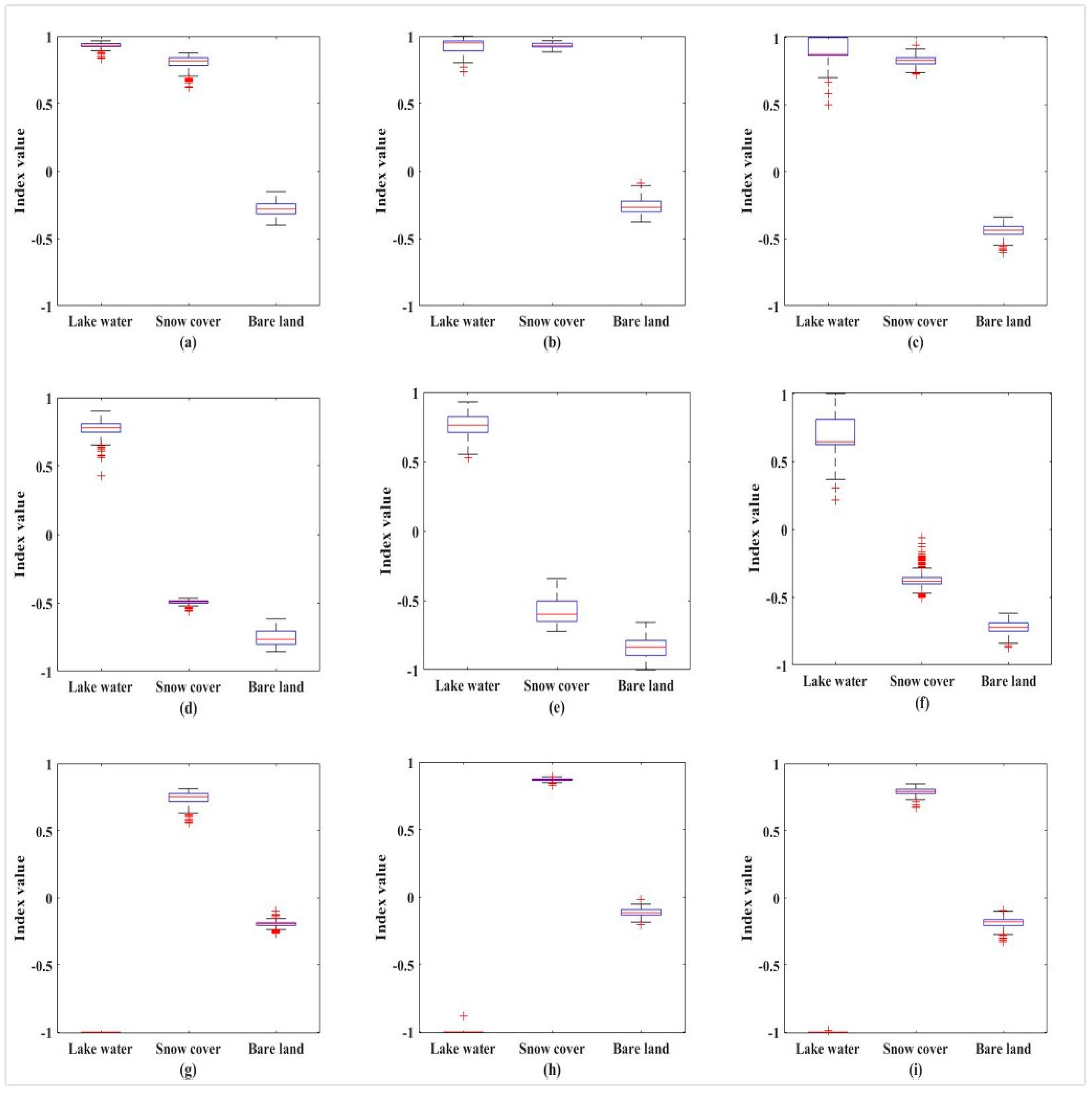
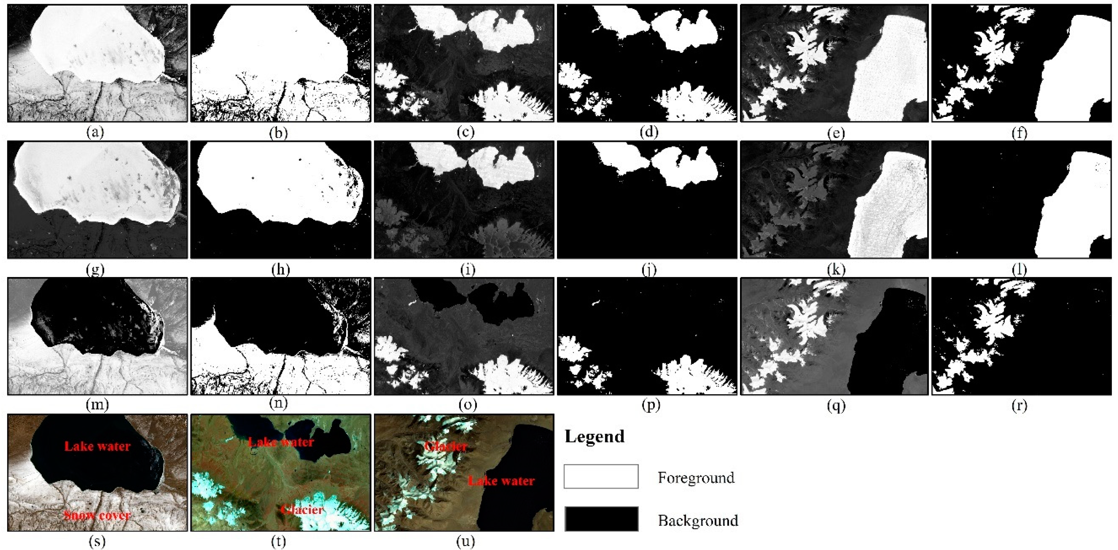
The performance of the NDSI/MNDWI and NDWIns in mapping lake water bodies with noise from SCG was tested and compared based on Landsat data in three study regions. It can be seen that both lake water bodies and SCG present high positive values in the NDSI/MNDWI image in Region I, II and III (Figure 5). This is because the reflectance of lake water bodies and SCG shows a downward trend from the green band to the SWIR1 band. As a result, the overall accuracy of the classified NDSI/MNDWI image is mainly influenced by the commission error from SCG in lake water bodies mapping (Table 5). Consequently, the NDSI/MNDWI has an overall accuracy of 78.8―83.8% in lake water bodies mapping and, thus, is not suitable to identify lake water bodies with noise from SCG (Table 5). Fortunately, it is apparent that the NDWIns enhances lake water with a positive value between 0.22―1.00 and suppresses the SCG information with negative values from −0.06 to −0.72 in Region I, II and III (Figure 5). This is because the reflectance of lake water bodies decreases steadily, while the reflectance of SCG remains stable in general or fluctuates slightly from the green band to NIR band (Figure 4). What is more, the NDWIns image exhibits negative values which are less than −0.5 in bare land areas (Figure 5). Consequently, with overall accuracies of 94.6―97.0% in lake water mapping (Table 5), the classified NDWIns image is capable of delineating lake water area bodies and suppressing SCG and bare land effectively (Figure 6). Therefore, the NDWIns is competent to identify lake water bodies from the background, including SCG.
3.3. SCG Mapping with Noise from Lake Water Using NDSI/MNDWI and NDSInw
The performance of the NDSI/MNDWI and NDSInw in mapping SCG with noise from lake water bodies was also tested and compared in Region I, II and III. In the NDSI/MNDWI image, both SCG and lake water have high positive values (Figure 5) and display a white tone (Figure 6) because of their similar variation tendency of spectral distributions from the green band to the SWIR1 band. The NDSI/MNDWI image overestimates SCG largely due to the commission error from lake water bodies and, thus, is not suitable to discriminate between lake water bodies and SCG. Consequently, the accuracy assessment reveals that NDSI/MNDWI is less capable of suppressing lake water areas in extracting SCG with overall accuracies of 71.5―86.5% (Table 6). However, the NDSInw image achieves a high positive value between 0.55–0.89 in SCG areas and a low negative value from −1.00 to −0.88 in lake water areas (Figure 5). This is because the reflectance of SCG falls dramatically from the NIR band to SWIR1 band, while the reflectance of lake water bodies which is lower than 0.05 remains unchanged in general or decreases slightly from the NIR band to SWIR1 band (Figure 4). In addition, the NDSInw image extracts negative values in bare land areas (Figure 5). As a result, the classified NDSInw image performs successfully in extracting SCG and suppressing lake water bodies and bare land with an overall accuracy of 94.9―97.0% (Figure 6; Table 6). Thus, the NDSInw can be suggested to extract SCG from the background, including lake water bodies.
It should be noted that the NDWI combining the green band and NIR band and the NDFSI normalizing the NIR band and SWIR2 band difference have the potential to identify lake water bodies from SCG and detect SCG from lake water bodies to some extent, respectively. This is because the difference of reflectance from the green band to NIR band in lake water areas is far greater than that in SCG areas, while the difference of reflectance between the NIR band and SWIR2 band in SCG areas is far higher than that in lake water areas (Figure 4).
Although the NDSInw image forfeits some SCG information by subtracting a positive value (0.05) from the difference between the NIR band and SWIR1 band, these losses can be considered negligible, owing to the high difference of reflectance between the NIR band and the SWIR1 band in SCG areas for NDSInw. Moreover, optimum thresholds which are supposed to be lower than the default threshold of NDSI can be found for NDSInw in distinguishing SCG from water bodies. This is because the mean index value of NDSInw is slightly lower than that of NDSI in SCG areas (Figure 5).
4. Discussion and Outlook
The accuracy of the index-based method in mapping the extents of lakes and SCG is primarily determined by the quality of the remote sensing data, e.g., clouds, terrain shadows and haze, which impact the spectral responses in the remote sensing imagery. To minimize the errors in water bodies detection, it is necessary to select satellite imagery with minimum contamination of cloud coverage and haze in the past [42], which limits the usage of most images to a great extent. Fortunately, several effective clouds and cloud-shadow mapping algorithms have been designed for the Landsat series [45,46,47]. It is promising to combine these methods with our new index-based methods to mitigate the negative effects inherited by satellite data.
In this study, only Landsat images were selected to demonstrate the performance of the new methods. Other similar optical sensors, such as the Sentinel-2, were not considered. However, as Sentinel-2 has similar spectral and spatial characteristics to Landsat OLI [48], their data have been combined to achieve a better temporal observation in the previous studies [47,49]. It is therefore worthwhile to test the sensitivity of other sensors for the reconstruction of time series of water resources product with high temporal resolution.
The combination of multispectral data and other kinds of remote sensing data provides new opportunities to detect temporal variations in land surface water bodies extent. For example, the Shuttle Radar Topography Missions Water Body Dataset and MODIS reflectance data were used to produce a new global land surface water map [50]. The Global Inland Water was produced using the Landsat reflectance data and elevation data [51]. Combining the land surface temperature and MODIS reflectance data, Pekel et al. (2014) mapped water bodies across Africa from 2004 to 2010 [52]. Lu et al. (2011) detected water bodies based on the Chinese HJ-1A/B satellites, slope information and the NIR band [53]. However, the main source of current products relies on the index-based methods from multispectral datasets to map the surface water bodies from the background [33]. In future, the combination of topography information, elevation data and land surface temperature with the newly developed water and snow indices in the present study is to be encouraged for better mapping of land surface water resources.
The threshold for land surface water bodies extraction is subjected to the user’s judgment according to different classification priorities [53]. Acceptable snow cover maps have been achieved with NDSI thresholds from 0.25 to 0.45 [24], while a default threshold of zero was suggested to separate water bodies from the background [25]. Thus, although the NDSI and MNDWI use the same equation, the suitable threshold of the NDSI/MNDWI is not a constant for snow cover mapping and land surface water bodies extraction. Besides, the determination of the threshold of the index-based method is largely dependent upon the study area. In regional water resources mapping, the Otsu’s threshold performs successfully to segment the foreground from the background. However, for large-scale regional land surface water bodies mapping, it is less capable of extracting all the water bodies from surrounding land features using one threshold [29]. Recently, Zhang et al. (2019) demonstrated that the NDSI threshold of 0.1 is more reasonable than the global NDSI threshold of 0.4 for monitoring snow cover using MODIS data in China [54]. Thus, a multi-threshold segmentation method is indispensable when the index-based methods are utilized in global water resource mapping.
Although the NDSInw method achieves high accuracy in open glaciers mapping in Regions II and III, it is difficult to extract information from glaciers covered by debris, which may influence the reflectance patterns of glaciers. In addition, the reflectance of water bodies is influenced by the concentration of sediment. The reflectance peak of water bodies moves to the longer wavelength with the increase of concentration of sediment. If the reflectance of water bodies in the NIR band was greater than that of the green band, the NDWIns will become invalid in this spectral reflection pattern. Thus, the NDWIns and NDSInw should be tested in other land covers and case study regions in future studies, and a and b in NDWIns and NDSInw should be adjusted in other special study sites to optimize their performance in extracting more accurate lake water bodies and SCG information.
By improving the existing water index and snow index, the NDWIns and NDSInw proposed in the present study open up new opportunities for evaluating the water quality and fractional snow cover, respectively. First, since the NDWI has been proven useful in evaluating water quality [22], it is therefore expected that NDWIns may also have a good application prospect in assessing water quality, such as suspended sediments and chlorophyll-a within a water body. Second, NDSInw opens up a new opportunity in calculating the percentage of snow cover in the pixel scale, as previous studies have already found a positive relationship between the old version snow index and fractional snow cover [28].
5. Conclusions
In this study, two new index-based methods were proposed based on the optimal band combination for improved discriminating between the lake water bodies and SCG in the Tibetan Plateau. Based on thorough evaluations using Landsat OLI, ETM+, and TM data, we show that NDWIns is highly effective in extracting lake water bodies and suppressing SCG information, while NDSInw demonstrates a proper capability of extracting SCG by ideally removing the contamination of water bodies. Overall, this study provides more appropriate methods for automatically distinguishing and extracting water bodies and SCG in an accurate manner over cold regions when compared with the traditional NDSI/MNDWI methods.
The main contribution of this study is to provide a new methodology for mapping different kinds of water resources, especially in discriminating between land surface water bodies and SCG. While the current validations focus only on certain areas in TP, it is believed that two new indices proposed in the present study will provide new chances for understanding the spatial and temporal patterns of different kinds of water resources. In particular, under the background of temperature rise and precipitation increase in the TP, the lakes and SCG in TP may be affected to a large extent. It is therefore expected to monitor changes in different kinds of water resources such as lake water bodies and SCG effectively over the entire TP with the help of the NDWIns and NDSInw, which improves understanding of the hydrological cycle and its responses to climate change in this region.
Author Contributions
D.Y., C.H., N.M., and Y.Z. jointly completed the study. The specific division of labor is as follows: conceptualization, D.Y.; methodology, D.Y.; software, D.Y. and C.H.; validation, D.Y.; formal analysis, C.H. and N.M.; investigation, D.Y. and N.M.; resources, D.Y.; writing—original draft preparation, D.Y. and N.M.; writing—review and editing, C.H. and Y.Z.; visualization, D.Y. and N.M.; supervision, Y.Z.; project administration, Y.Z.; funding acquisition, Y.Z. All authors have read and agreed to the published version of the manuscript.
Funding
This research was jointly funded by the National Key Research and Development Program of China (2017YFA0603101), the National Natural Science Foundation of China (41801051), Strategic Priority Research Program (A) of CAS (XDA20060201), the Research Funding of the China-Pakistan Joint Research Center for Earth Science, and the Open Research Fund Program of State Key Laboratory of Cryospheric Science, Northwest Institute of Eco-Environment and Resources, CAS (SKLCS-OP-2020-11). The authors thank the United States Geological Survey for free Landsat data.
Acknowledgments
The authors thank the three anonymous reviewers for their helpful comments.
Conflicts of Interest
No potential conflict of interest was reported by the authors.
References
- Huang, C.; Chen, Y.; Zhang, S.; Wu, J. Detecting, extracting, and monitoring surface water from space using optical sensors: A review. Rev. Geophys. 2018, 56, 333–360. [Google Scholar] [CrossRef]
- Biemans, H.; Siderius, C.; Lutz, A.F.; Nepal, S.; Ahmad, B.; Hassan, T.; von Bloh, W.; Wijngaard, R.R.; Wester, P.; Shrestha, A.B.; et al. Importance of snow and glacier meltwater for agriculture on the Indo-Gangetic Plain. Nature Sustain. 2019, 2, 594–601. [Google Scholar] [CrossRef]
- Busker, T.; Roo, A.D.; Gelati, E.; Schwatke, C.; Adamovic, M.; Bisselink, B.; Pekel, J.; Cottam, A. A global lake and reservoir volume analysis using a surface water dataset and satellite altimetry. Hydrol. Earth Syst. Sci. 2019, 23, 669–690. [Google Scholar] [CrossRef] [Green Version]
- Yao, T.; Thompson, L.G.; Mosbrugger, V.; Zhang, F.; Ma, Y.; Luo, T.; Xu, B.; Yang, X.; Joswiak, D.R.; Wang, W.; et al. Third pole environment (TPE). Environ. Dev. 2012, 3, 52–64. [Google Scholar] [CrossRef]
- Qiu, J. China: The third pole. Nature 2008, 454, 393–396. [Google Scholar] [CrossRef] [Green Version]
- Yao, T.; Xue, Y.; Chen, D.; Chen, F.; Thompson, L.; Cui, P.; Koike, T.; Lau, W.K.M.; Lettenmaier, D.; Mosbrugger, V.; et al. Recent Third Pole’s Rapid Warming Accompanies Cryospheric Melt and Water Cycle Intensification and Interactions between Monsoon and Environment: Multidisciplinary Approach with Observations, Modeling, and Analysis. Bull. Am. Meteorol. Soc. 2019, 100, 423–444. [Google Scholar] [CrossRef]
- Yao, T.; Thompson, L.G.; Yang, W.; Yu, W.; Gao, Y.; Guo, X.; Yang, X.; Duan, K.; Zhao, H.; Xu, B.; et al. Different glacier status with atmospheric circulations in Tibetan Plateau and surroundings. Nat. Clim. Chang. 2012, 2, 663–667. [Google Scholar] [CrossRef]
- Yang, K.; Wu, H.; Qin, J.; Lin, C.; Tang, W.; Chen, Y. Recent climate changes over the Tibetan Plateau and their impacts on energy and water cycle: A review. Glob. Planet. Chang. 2014, 112, 79–91. [Google Scholar] [CrossRef]
- Zhang, G. Increased mass over the Tibetan Plateau: From lakes or glaciers? Geophys. Res. Lett. 2013, 40, 1–6. [Google Scholar] [CrossRef]
- Zhang, G.; Yao, T.; Chen, W.; Zheng, G.; Shum, C.K.; Yang, K.; Piao, S.; Sheng, Y.; Yi, S.; Li, J.; et al. Regional differences of lake evolution across China during 1960-2015 and its natural and anthropogenic causes. Remote Sens. Environ. 2019, 221, 386–404. [Google Scholar] [CrossRef]
- Zhang, G.; Yao, T.; Piao, S.; Bolch, T.; Xie, H.; Chen, D.; Gao, Y.; O’Reilly, C.M.; Shum, C.K.; Yang, K.; et al. Extensive and drastically different alpine lake changes on Asia’s high plateaus during the past four decades. Geophys. Res. Lett. 2017, 44, 252–260. [Google Scholar] [CrossRef] [Green Version]
- Kang, S.; Xu, Y.; You, Q.; Flüge, W.; Pepin, N.; Yao, T. Review of climate and cryospheric change in the Tibetan Plateau. Environ. Res. Lett. 2010, 5, 015101. [Google Scholar] [CrossRef]
- Alexander, L.V.; Allen, S.K.; Bindoff, N.L.; Breon, F.-M.; Church, J.A.; Cubasch, U.; Emori, S.; Forster, P.; Friedlingstein, P.; Gillett, N. Summary for Policymakers; IMAS Research and Education Centre: Cambridge, UK, 2013. [Google Scholar]
- Wang, J.; Song, C.; Reager, J.T.; Yao, F.; Famiglietti, J.S.; Sheng, Y.; MacDonald, G.M.; Brun, F.; Schmied, H.M.; Marston, R.A.; et al. Recent global decline in endorheic basin water storages. Nat. Geosci. 2018, 11, 926–932. [Google Scholar] [CrossRef] [PubMed] [Green Version]
- Immerzeel, W.W.; Lutz, A.F.; Andrade, M.; Bahl, A.; Biemans, H.; Bolch, T.; Hyde, S.; Brumby, S.; Davies, B.J.; Elmore, A.C.; et al. Importance and vulnerability of the world’s water towers. Nature 2020, 577, 364–369. [Google Scholar] [CrossRef] [PubMed]
- Chen, D.L.; Xu, B.; Yao, T.; Guo, Z.; Cui, P.; Chen, F.; Zhang, R.; Zhang, X.; Zhang, Y.; Fan, J.; et al. Assessment of past, present and future environmental changes on the Tibetan Plateau. Chin. Sci. Bull. 2015, 60, 3025–3035. [Google Scholar]
- Ma, N.; Szilagyi, J.; Niu, G.Y.; Zhang, Y.; Zhang, T.; Wang, B.; Wu, Y. Evaporation variability of Nam Co lake in the Tibetan Plateau and its role in recent rapid lake expansion. J. Hydrol. 2016, 537, 27–35. [Google Scholar] [CrossRef]
- Zhang, Y.; Ma, N. Spatiotemporal variability of snow cover and snow water equivalent in the last three decades over Eurasia. J. Hydrol. 2018, 559, 238–251. [Google Scholar] [CrossRef]
- You, Q.; Wu, T.; Shen, L.; Pepin, N.; Zhang, L.; Jiang, Z.; Wu, Z.; Kang, S.; AghaKouchak, A. Review of snow cover variation over the Tibetan Plateau and its influence on the broad climate system. Earth-Sci. Rev. 2020, 201, 103043. [Google Scholar] [CrossRef]
- Zhang, G.; Li, J.; Zheng, G. Lake-area mapping in the Tibetan Plateau: An evaluation of data and methods. Int. J. Remote Sens. 2016, 38, 742–772. [Google Scholar] [CrossRef]
- Brown, R.D.; Robinson, D.A. Northern Hemisphere spring snow cover variability and change over 1922–2010 including an assessment of uncertainty. Cryosphere 2011, 5, 219–229. [Google Scholar] [CrossRef] [Green Version]
- McFeeters, S.K. The use of the Normalized Difference Water Index (NDWI) in the Delineation of Open Water Features. Int. J. Remote Sens. 1996, 17, 1425–1432. [Google Scholar] [CrossRef]
- Negi, H.S.; Singh, S.K.; Kulkarni, A.V.; Semwal, B.S. Field-based spectral reflectance measurements of seasonal snow cover in the Indian Himalaya. Int. J. Remote Sens. 2010, 31, 2393–2417. [Google Scholar] [CrossRef]
- Hall, D.K.; Riggs, G.A.; Salomonson, V.V. Development of methods for mapping global snow cover using moderate resolution imaging spectoradiometer data. Remote Sens. Environ. 1995, 54, 127–140. [Google Scholar] [CrossRef]
- Xu, H. Modification of Normalized Difference Water Index (NDWI) to Enhance Open Water Features in Remotely Sensed Imagery. Int. J. Remote Sens. 2006, 27, 3025–3033. [Google Scholar] [CrossRef]
- Wang, X.Y.; Wang, J.; Jiang, Z.Y.; Li, H.Y.; Hao, X.H. An effective method for snow-cover mapping of dense coniferous forests in the upper Heihe River Basin using Landsat Operational Land Imager Data. Remote Sens. (Basel) 2015, 7, 17246–17257. [Google Scholar] [CrossRef] [Green Version]
- Ouma, Y.O.; Tateishi, R. A water index for rapid mapping of shoreline changes of five East African Rift Valley lakes: An empirical analysis using Landsat TM and ETM+ data. Int. J. Remote Sens. 2006, 27, 3153–3181. [Google Scholar] [CrossRef]
- Salomonson, V.V.; Appel, I. Development of the Aqua MODIS NDSI fractional snow cover algorithm and validation results. IEEE. Trans. Geosci. Remote 2006, 44, 1747–1756. [Google Scholar] [CrossRef]
- Li, W.; Du, Z.; Ling, F.; Zhou, D.; Wang, H.; Gui, Y.; Sun, B.; Zhang, X. A Comparison of Land surface water mapping using the normalized difference water index from TM, ETM+ and ALI. Remote Sens. (Basel) 2013, 5, 5530–5549. [Google Scholar] [CrossRef] [Green Version]
- Rogers, A.S.; Kearney, M.S. Reducing Signature Variability in Unmixing Coastal Marsh Thematic Mapper Scenes Using Spectral Indices. Remote Sens. (Basel) 2004, 25, 2317–2335. [Google Scholar] [CrossRef]
- Xiao, X.; Shen, Z.; Qin, X. Assessing the potential of vegetation sensor data for mapping snow and ice cover: A normalized difference snow and ice index. Int. J. Remote Sens. 2001, 22, 2479–2487. [Google Scholar] [CrossRef]
- Yamazaki, D.; Trigg, M.A. Hydrology: The dynamics of Earth’s surface water. Nature 2016, 540, 348–349. [Google Scholar] [CrossRef] [PubMed] [Green Version]
- Khandelwal, A.; Karpatne, A.; Marlier, M.E.; Kim, J.; Lettenmaier, D.P.; Kumar, V. An approach for global monitoring of surface water extent variations in reservoirs using MODIS data. Remote Sens. Environ. 2017, 202, 113–128. [Google Scholar] [CrossRef]
- Crane, R.G.; Andersen, K.R. Satellite discrimination of snow/cloud surfaces. Int. J. Remote Sens. 1984, 5, 213–223. [Google Scholar] [CrossRef]
- Marchane, A.; Jarlan, L.; Hanich, L.; Boudhar, A.; Gascoin, S.; Tavernier, A.; Filali, N.; Le Page, M.; Hagolle, O.; Berjamy, B. Assessment of daily MODIS snow cover products to monitor snow cover dynamics over the Moroccan Atlas mountain range. Remote Sens. Environ. 2015, 160, 72–86. [Google Scholar] [CrossRef]
- Shimamura, Y.; Izumi, T.; Matsuyama, H. Evaluation of a useful method to identify snow-covered areas under vegetation–comparisons among a newly proposed snow index, normalized difference snow index, and visible reflectance. Int. J. Remote Sens. 2006, 27, 4867–4884. [Google Scholar] [CrossRef]
- Gao, B.C. A normalized difference water index for remote sensing of vegetation liquid water from space. Remote. Sens. Environ. 1996, 58, 257–266. [Google Scholar] [CrossRef]
- Feyisa, G.L.; Meilby, H.; Fensholt, R.; Pround, S.R. Automated Water Extraction Index: A new technique for surface water mapping using Landsat imagery. Remote Sens. Environ. 2014, 140, 23–35. [Google Scholar] [CrossRef]
- Du, Z.; Li, W.; Zhou, D.; Tian, L.; Ling, F.; Wang, H.; Gui, Y.; Sun, B. Analysis of Landsat-8 OLI imagery for Land Surface Water Mapping. Remote Sens. Lett. 2014, 5, 672–681. [Google Scholar] [CrossRef]
- Otsu, N. A Threshold Selection Method from Gray-Level Histograms. IEEE Trans. Syst. Man Cybern. B 1979, 9, 62–66. [Google Scholar] [CrossRef] [Green Version]
- Fisher, A.; Flood, N.; Danaher, T. Comparing Landsat water index methods for automated water classification in eastern Australia. Remote Sens. Environ. 2016, 175, 167–182. [Google Scholar] [CrossRef]
- Verpoorter, C.; Kutser, T.; Tranvik, L. Automated mapping of water bodies using Landsat multispectral data. Limnol. Oceanogr-Meth. 2012, 10, 1037–1050. [Google Scholar] [CrossRef]
- Tarpanelli, A.; Amarnath, G.; Brocca, L.; Massari, C.; Moramarco, T. Discharge estimation and forecasting by MODIS and altimetry data in Niger-Benue River. Remote Sens. Environ. 2017, 195, 96–106. [Google Scholar] [CrossRef]
- Zhang, H.; Zhang, F.; Che, T.; Wang, S. Comparative evaluation of VIIRS daily snow cover product with MODIS for snow detection in China based on ground observations. Sci. Total Environ. 2020, 724, 138156. [Google Scholar] [CrossRef]
- Goodwin, N.R.; Collett, L.J.; Denham, R.J.; Flood, N.; Tindall, D. Cloud and cloud shadow screening across Queensland, Australia: An automated method using Landsat TM/ETM+ time series. Remote Sens. Environ. 2013, 134, 50–65. [Google Scholar] [CrossRef]
- Zhu, Z.; Woodcock, C.E. Automated cloud, cloud shadow, and snow detection in multitemporal Landsat data: An algorithm designed specifically for monitoring land cover change. Remote Sens. Environ. 2014, 152, 217–234. [Google Scholar] [CrossRef]
- Zhu, Z.; Wang, S.; Woodcock, C.E. Improvement and expansion of the Fmask algorithm: Cloud, cloud shadow, and snow detection for Landsats 4–7, 8, and Sentinel 2 images. Remote Sens. Environ. 2015, 159, 269–277. [Google Scholar] [CrossRef]
- Storey, J.; Roy, D.P.; Masek, J.; Gascon, F.; Dwyer, J.; Choate, M. A note on the temporary misregistration of Landsat-8 Operational Land Imager (OLI) and Sentinel-2 Multi Spectral Instrument (MSI) imagery. Remote Sens. Environ. 2016, 186, 121–122. [Google Scholar] [CrossRef] [Green Version]
- Novelli, A.; Aguilar, M.A.; Nemmaoui, A.; Aguilar, F.J.; Tarantino, E. Performance evaluation of object based greenhouse detection from Sentinel-2 MSI and Landsat 8 OLI data: A case study from Almería (Spain). Int. J. Appl. Earth Obs. 2016, 52, 403–411. [Google Scholar] [CrossRef] [Green Version]
- Carroll, M.L.; Townshend, J.R.; DiMiceli, C.M.; Noojipady, P.; Sohlberg, R.A. A new global raster water mask at 250 m resolution. Int. J. Digit. Earth 2009, 2, 291–308. [Google Scholar] [CrossRef]
- Feng, M.; Sexton, J.O.; Channan, S.; Townshend, J.R. A global, high-resolution (30-m) inland water body dataset for 2000: First results of a topographic—Spectral classification algorithm. Int. J. Digit. Earth 2014, 9, 113–133. [Google Scholar] [CrossRef] [Green Version]
- Pekel, J.F.; Vancutsem, C.; Bastin, L.; Clerici, M.; Vanbogaert, E.; Bartholomé, E.; Defourny, P. A near real-time water surface detection method based on HSV transformation of MODIS multi-spectral time series data. Remote Sens. Environ. 2014, 140, 704–716. [Google Scholar] [CrossRef] [Green Version]
- Lu, S.; Wu, B.; Yan, N.; Wang, H. Water body mapping method with HJ-1A/B satellite imagery. Int. J. Appl. Earth Obs. 2011, 13, 428–433. [Google Scholar] [CrossRef]
- Zhang, H.; Zhang, F.; Zhang, G.; Che, T.; Yan, M.; Ma, N. Ground-based evaluation of MODIS snow cover product V6 across china: Implications for the selection of NDSI threshold. Sci. Total Environ. 2019, 651, 2712–2716. [Google Scholar] [CrossRef] [PubMed]
Figure 1.
Geographical distribution of lakes and glaciers in the Tibetan Plateau.

Figure 2.
(a) the Tibetan Plateau; (b) Landsat-7 ETM+ image (RGB:321; Region II); (c) Landsat-5 TM image (RGB:321; Region III); (d) Landsat-8 OLI image (RGB:432; Region I).
Figure 2.
(a) the Tibetan Plateau; (b) Landsat-7 ETM+ image (RGB:321; Region II); (c) Landsat-5 TM image (RGB:321; Region III); (d) Landsat-8 OLI image (RGB:432; Region I).

Figure 3.
Flowchart of methodology.

Figure 4.
Reflectance distribution of three land cover types in three study regions. (a–c) are the reflectance distribution of lake water in Region I, II and III; (d) is the reflectance distribution of snow cover in Region I; (e,f) are the reflectance distribution of glacier in Region II and III; (g–i) are the reflectance distribution of bare land in Region I, II and III.

Figure 5.
The index values in three study regions based on three hundred sample points. (a–c) are the NDSI/MNDWI value in Region I, II and III; (d–f) are the NDWIns value in Region I, II and III; (g–i) are the NDSInw value in Region I, II and III.
Figure 5.
The index values in three study regions based on three hundred sample points. (a–c) are the NDSI/MNDWI value in Region I, II and III; (d–f) are the NDWIns value in Region I, II and III; (g–i) are the NDSInw value in Region I, II and III.

Figure 6.
The index images and classified images. (a,c,e) are the NDSI/MNDWI image in region I, II and III; (b,d,f) are classified NDSI/MNDWI image in region I, II and III; (g,i,k) are the NDWIns image in region I, II and III; (h,j,l) are classified NDWIns image in region I, II and III; (m,o,q) are the NDSInw image in region I, II and III; (n,p,r) are classified NDSInw image in region I, II and III; (s) Landsat-8 OLI image in Region I (RGB:432); (t) Landsat-7 ETM+ image in Region II (RGB:321); (u) Landsat-5 TM image in Region III (RGB:321).


Table 1.
Basic characteristics of Landsat Operational Land Imager (OLI), Enhanced Thematic Mapper Plus (ETM+) and Thematic Mapper (TM) data.
Table 1.
Basic characteristics of Landsat Operational Land Imager (OLI), Enhanced Thematic Mapper Plus (ETM+) and Thematic Mapper (TM) data.
| Landsat OLI | Landsat ETM+ | Landsat TM | |||
|---|---|---|---|---|---|
| Band Name | Wavelength Range (μm) | Band Name | Wavelength Range (μm) | Band Name | Wavelength Range (μm) |
| B1-Deep Blue | 0.433–0.453 | ||||
| B2-Blue | 0.450–0.515 | B1-Blue | 0.450–0.515 | B1-Blue | 0.45–0.52 |
| B3-Green | 0.525–0.600 | B2-Green | 0.525–0.605 | B2-Green | 0.52–0.60 |
| B4-Red | 0.630–0.680 | B3-Red | 0.630–0.690 | B3-Red | 0.63–0.69 |
| B5-NIR | 0.845–0.885 | B4-NIR | 0.775–0.900 | B4-NIR | 0.76–0.90 |
| B6-SWIR1 | 1.560–1.660 | B5-SWIR1 | 1.550–1.750 | B5-SWIR1 | 1.55–1.75 |
| B7-SWIR2 | 2.100–2.300 | B7-SWIR2 | 2.090–2.350 | B7-SWIR2 | 2.08–2.35 |
Table 2.
Definition of each index (NDI is normalized difference index; ρbandx is the reflectance of the xth band).
Table 2.
Definition of each index (NDI is normalized difference index; ρbandx is the reflectance of the xth band).
| Sensor | Basic Formula of Each Index |
|---|---|
| OLI | NDI53 = (ρband3 − ρband5)/(ρband3 + ρband5); NDI63 = (ρband3 − ρband6)/(ρband3 + ρband6) |
| NDI73 = (ρband3 − ρband7)/(ρband3 + ρband7); NDI64 = (ρband4 − ρband6)/(ρband4 + ρband6) | |
| NDI65 = (ρband5 − ρband6)/(ρband5 + ρband6) | |
| TM/ETM+ | NDI42 = (ρband2 − ρband4)/(ρband2 + ρband4); NDI52 = (ρband2 − ρband5)/(ρband2 + ρband5) |
| NDI72 = (ρband2 − ρband7)/(ρband2 + ρband7); NDI53 = (ρband3 − ρband5)/(ρband3 + ρband5) | |
| NDI54 = (ρband4 − ρband5)/(ρband4 + ρband5) |
Table 3.
Confusion matrix of sample points Nij. Classified binary images are in rows and the corresponding reference points are in columns. N11, N12, N21, N22 are the sample counts between classified binary image and reference point.
Table 3.
Confusion matrix of sample points Nij. Classified binary images are in rows and the corresponding reference points are in columns. N11, N12, N21, N22 are the sample counts between classified binary image and reference point.
| Class | SCG | Non-SCG | Non-SCG |
| SCG | N11 | N12 | N1j |
| Non-SCG | N21 | N22 | N2j |
| Total | Ni1 | Ni2 | N |
| Class | Lake Water | Non-Lake Water | Total |
| Lake water | N11 | N12 | N1j |
| Non-Lake water | N21 | N22 | N2j |
| Total | Ni1 | Ni2 | N |
Table 4.
The contrast values (CV) of five indices between lake water and snow cover/glaciers (SCG).
| Sensor | Mean Values or CV | NDI53 | NDI63 | NDI73 | NDI64 | NDI65 |
| OLI | Mean value of Lake Water | 0.844 | 0.922 | 0.928 | 0.737 | 0.354 |
| Mean value of Snow Cover | 0.006 | 0.832 | 0.826 | 0.837 | 0.831 | |
| CV (Lake Water − Snow cover) | 0.838 | 0.090 | 0.102 | −0.100 | −0.477 | |
| CV (Snow cover − Lake Water) | −0.838 | −0.090 | −0.102 | 0.100 | 0.477 | |
| Sensor | Mean Values or CV | NDI42 | NDI52 | NDI72 | NDI53 | NDI54 |
| ETM+ | Mean value of Lake Water | 0.817 | 0.933 | 0.931 | 0.744 | 0.541 |
| Mean value of Glacier | −0.054 | 0.928 | 0.945 | 0.921 | 0.935 | |
| CV (Lake Water − Glacier) | 0.871 | 0.005 | −0.014 | −0.177 | −0.394 | |
| CV (Glacier − Lake water) | −0.871 | −0.005 | 0.014 | 0.177 | 0.394 | |
| Sensor | Mean Values or CV | NDI42 | NDI52 | NDI72 | NDI53 | NDI54 |
| TM | Mean value of Lake Water | 0.692 | 0.877 | 0.871 | 0.710 | 0.471 |
| Mean value of Glacier | 0.073 | 0.871 | 0.904 | 0.864 | 0.852 | |
| CV (Lake Water − Glacier) | 0.619 | 0.006 | −0.033 | −0.154 | −0.381 | |
| CV (Glacier − Lake water) | −0.619 | −0.006 | 0.033 | 0.154 | 0.381 |
Table 5.
The extraction accuracy of lake water from SCG.
| Method | Region | Thres- Hold | Commission Error (%) | Omission Error (%) | Overall Accuracy (%) | Kappa Coefficient |
|---|---|---|---|---|---|---|
| NDSI/MNDWI | I | 0.38 | 27.36 | 0.27 | 82.7 | 0.6607 |
| II | 0.33 | 28.80 | 7.68 | 83.8 | 0.6698 | |
| III | 0.31 | 30.40 | 13.75 | 78.8 | 0.5782 | |
| NDWIns | I | 0.09 | 0.25 | 10.34 | 95.2 | 0.9018 |
| II | −0.01 | 1.06 | 7.40 | 97.0 | 0.9335 | |
| III | −0.02 | 0.74 | 12.36 | 94.6 | 0.8874 |
Table 6.
The extraction accuracy of SCG from lake water bodies.
| Method | Region | Thres- Hold | Commission Error (%) | Omission Error (%) | Overall Accuracy (%) | Kappa Coefficient |
|---|---|---|---|---|---|---|
| NDSI/MNDWI | I | 0.38 | 43.56 | 6.17 | 71.5 | 0.4605 |
| II | 0.33 | 38.43 | 11.40 | 86.5 | 0.6405 | |
| III | 0.31 | 26.78 | 2.87 | 81.7 | 0.6360 | |
| NDSInw | I | 0.32 | 2.20 | 6.72 | 96.8 | 0.9301 |
| II | 0.27 | 6.70 | 11.66 | 94.9 | 0.8724 | |
| III | 0.11 | 4.16 | 2.04 | 97.0 | 0.9396 |
© 2020 by the authors. Licensee MDPI, Basel, Switzerland. This article is an open access article distributed under the terms and conditions of the Creative Commons Attribution (CC BY) license (http://creativecommons.org/licenses/by/4.0/).
Share and Cite
MDPI and ACS Style
Yan, D.; Huang, C.; Ma, N.; Zhang, Y. Improved Landsat-Based Water and Snow Indices for Extracting Lake and Snow Cover/Glacier in the Tibetan Plateau. Water 2020, 12, 1339. https://doi.org/10.3390/w12051339
AMA Style
Yan D, Huang C, Ma N, Zhang Y. Improved Landsat-Based Water and Snow Indices for Extracting Lake and Snow Cover/Glacier in the Tibetan Plateau. Water. 2020; 12(5):1339. https://doi.org/10.3390/w12051339
Chicago/Turabian StyleYan, Dajiang, Chang Huang, Ning Ma, and Yinsheng Zhang. 2020. "Improved Landsat-Based Water and Snow Indices for Extracting Lake and Snow Cover/Glacier in the Tibetan Plateau" Water 12, no. 5: 1339. https://doi.org/10.3390/w12051339
Note that from the first issue of 2016, this journal uses article numbers instead of page numbers. See further details here.