Modeling Improved Performance of Reduced-Height Biosand Water Filter Designs


1
Department of Chemical Engineering, University of Florida, Gainesville, FL 32611, USA
2
Soil and Water Sciences Department, University of Florida, Gainesville, FL 32611, USA
*
Author to whom correspondence should be addressed.
Water 2020, 12(5), 1337; https://doi.org/10.3390/w12051337
Submission received: 27 March 2020
/
Revised: 1 May 2020
/
Accepted: 4 May 2020
/
Published: 8 May 2020
(This article belongs to the Special Issue Point-of-Use Water Treatment)
Abstract
:Point-of-use biosand water filters are widely distributed in undeveloped or developing regions due to their water treatment success and low-cost design, but two gaps remain in the basic technology: (1) the filter body is oversized relative to its contaminant removal performance, and (2) the heavy design largely excludes difficult to reach locations in need of clean water solutions. Here, we model design modifications to the v.10 Centre for Affordable Water and Sanitation Technology biosand filter using a reduced filter height, increased biolayer area, and conserved reservoir volume. We compare the hydraulic characteristics (dynamic velocity and head pressure) and percent contaminant removal of bacteria Escherichia coli and virus MS2 of the modified designs to the traditional control design using a finite element approximation of Darcy’s law with discrete time steps and a slow-sand filtration model. We demonstrate that a reduced-height design has a greater impact on contaminant removal compared to the traditional design (largely due to the increased residence time from the decreased flow rate inside the filter). For example, our 70% reduced-height filter design removed 99.5% and 73.93% of E. coli and MS2, respectively, where the traditional filter design removed 62.81% and 27.6%, respectively. Reduced-height designs should be pursued as a viable solution to improve filter performance while allowing for alternative construction techniques with greater end-user accessibility compared to the traditional design.
1. Introduction
Nearly 10% of the world’s population (785 million people) still used an unprotected or untreated water source in 2017, with the largest concentration of inadequate water supplies in undeveloped areas [1]. A contributing factor to this global inadequacy is that many developing countries lack practical water treatment solutions, with large populations having little or no access to proper water treatment facilities. One popular household-scale water treatment (HWT) solution common in these impacted areas is the biosand water filter (BSF); over 650,000 have been distributed since its introduction in the early 1990s [2,3]. As one of the most effective and simplest water treatment options, biosand filtration offers many advantages compared to other conventional HWT systems such as a high flow rate [4], user-friendly operation [5], low material and production cost [2], successful performance (e.g., nearly 99% removal of harmful bacteria and 70% of viruses from the contaminated water; [6,7,8]), an active biolayer that strengthens over time [9], and proven health benefits (e.g., reduced cases of diarrhea) [10]. However, there are two inherent gaps in the current BSF design: (1) the filter body is oversized relative to its contaminant removal performance (i.e., the filter can be reduced in size with the same removal results) and (2) the heavy design (350 lbs per filter) largely excludes difficult to reach locations which are often the most in need of a HWT solution.
Several other options for HWT systems have been explored to help overcome the BSF gaps [5,9] such as solar disinfection [11], chlorination [12], ceramic filtration [13], and activated charcoal filtration [14], but these methods also have their own inherent design and knowledge gaps. For example, solar disinfection relies heavily on specific uncontrollable environmental factors and is at a greater disadvantage than other HWT techniques [11], chlorination requires access to outside resources and may pose certain long-term health effects [4,12], ceramic filtration has a very low flow rate, is ineffective after three years, has uncharacterized viral removal capabilities, and has a high up-front cost [2,13,15], and activated charcoal filtration has a short service life and is ineffective against certain types of viruses [14]. As a result, the BSF remains a widely adopted solution for basic water treatment, despite its inherent gaps.
As for the size of the BSF, past studies have shown that nearly 99% of bacteria removal occurs in just the top 5 cm of the filter media [16,17], yet the filter media in the traditional BSF design is packed to a depth of 55 cm (i.e., 89% of the filter media may only contribute an additional 1% removal of bacteria) [6]. This oversized filter contributes to its bulky weight [4] and, even when constructed on site, heavy materials not available in remote areas (e.g., concrete mix) must be transported from populated areas [9]. Because of the educational, accessibility, and operational issues, many communities have refused to fully adopt these filters and instead revert to drinking contaminated water [18,19]. A modified, reduced height and weight model of the BSF could help mitigate these issues, providing clean water for populations still suffering from poor water quality.
However, knowledge gaps have prevented filter modifications from becoming a practical consideration, despite the expected benefits of a modified design and its impact on a global society. For example, (1) there is still limited understanding of the exact relationship between the removal efficiency of microorganisms of the BSF and parameters such as fluid velocity, grain size, sand bed depth, temperature, and the age of the biolayer (also referred to as the Schmutzdecke; [20]), and (2) there are few mathematical models relevant to the BSF to develop an accurate relationship between the removal of harmful contaminants and its operating conditions. Previous studies have observed a lower removal efficiency as grain size and velocity have increased [7,21,22], and others have shown a positive correlation between removal efficiency and the temperature of the water [20], age of the biolayer [8], and sand bed depth [23,24]. Yet, these trends are still uncharacterized for alternative BSF designs. Here, we apply colloid filtration theory [25,26], with an incorporated biolayer (Schmutzdecke) term first introduced by Schijven et al. (2013) and later developed by Vissink (2016), to model alternative BSF parameters (e.g., filter size, grain size, velocity, sand bed depth, and biolayer age) to evaluate the impacts of BSF design modifications [20,27].
In this study, we model the hydraulic and contaminant removal dynamics within (1) the traditional BSF design, (2) a 40% reduced-height design, and (3) a 70% reduced-height design to identify the performance of design modifications focused on maximizing the biolayer area (where nearly all contaminant removal is documented to occur; [9,17]) and reducing inefficient (i.e., limited contaminant removal) regions within the traditional BSF. We first used a finite element approximation of Darcy’s law with discrete time steps to establish the flow rates throughout each filter. We then used a slow-sand filtration model to characterize and estimate the contaminant removal within each BSF design. Contaminant removal results are specifically modeled for the Escherichia coli (E. coli) bacteria and MS2 virus. Specifically, results from this study can be used to improve the BSF design for future applications, while laying a groundwork for advances in construction and distribution, which ultimately can improve unsuitable water supplies for many communities in remote regions of the world.
2. Materials and Methods
2.1. Biosand Filter Overview
The traditional BSF design can be divided into four main components: (1) the filter body, (2) sand and gravel inside the filter (referred to here as the effective area), (3) the active biolayer that occupies the standing water surface above the effective area and may penetrate slightly into the uppermost portion of the effective area, and (4) the reservoir area above the biolayer which serves as storage for contaminated water and establishes head pressure when occupied with water. In sequence, contaminated water is first poured into the top of the filter and fills the reservoir area. This water then passes through a diffuser plate and mixes with the biolayer where microbial activity removes contaminants from the soiled water. Water then infiltrates due to gravity into the effective area and moves downward through the filter. As water continues through the effective area (i.e., sand), particles are further removed by screening, adsorption, and natural death among other processes [28]. Ultimately, clean water is discharged through an outlet pipe and collected by the user. Flow through the traditional BSF can be characterized as anisotropic, with a heterogeneous media bed (medium to fine sand top layer, coarse sand middle layer, and gravel bottom layer) [6].
Most notable to the filter is the biolayer which accumulates along the surface of the top sand layer and matures over time as contaminated influent provides new sources of microbes and nutrients. As the microbial ecosystem develops, influent bacteria and viruses undergo a series of chemical and biological degradations while passing through the biolayer including physical straining [28,29,30,31]; this process is the driving contaminant removal mechanism for the BSF. The biolayer exists because the filter outlet height is slightly above the surface of the effective area to prevent the microbial community from drying out. This is particularly important given that the BSF is inherently an intermittent system as users typically charge the filter one time to a few times per day. Lastly, the BSF is recognized for its easy cleaning, as the surface of the effective layer can be scraped, stirred, or raked as pore spaces become too clogged and the flow rates too slow; the filter can also be emptied and repacked, which further prevents against channeling or preferential flow path issues that may otherwise develop over time.
2.2. Design Simplification
There are three media layers in the traditional filter design (from top to bottom): fine to medium sand, coarse sand, and gravel. Since the BSF is gravity driven, the flow rate is then controlled by the media layer with the lowest hydraulic conductivity (i.e., the top layer of fine to medium sand). This renders the other two layers (coarse sand and gravel) negligible in their flow rate impact [32]. These layers are also negligible in their impact on contaminant removal [28]. Currently, the traditional design is capable of removing nearly 100% of all bacterial contaminants [6,22], but this efficiency varies for different filter properties such as media grain size, fluid velocity, and depth of the sand bed [16,21,23,24]. Table 1 summarizes the documented percent bacteria removal through the traditional BSF with depth, further confirming that nearly all removal occurs through the biolayer. Given these results, we hypothesized the BSF could achieve the same removal rates with a drastic reduction in overall sand depth. For the alternate BSF designs modeled in this study, we have removed the bottom two coarse layers found in the traditional design to conserve available effective area and reduce the required materials for construction while presumably having no effect on the overall contaminant removal inside the filter.
2.3. Experimental Design and Conditions
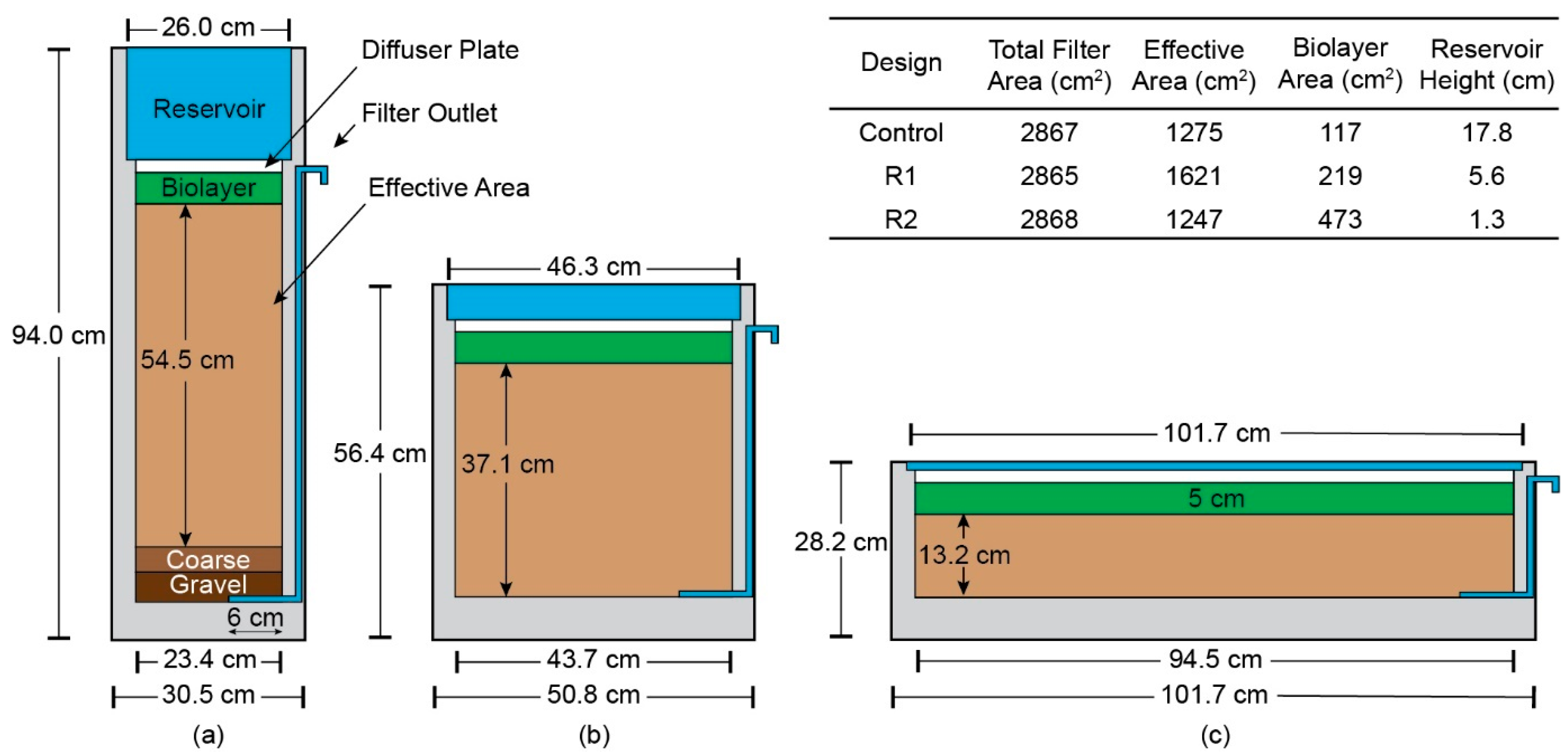
We analyzed three different filter designs: (1) the traditional BSF (control), (2) a 40% reduced-height design (R1), and (3) a 70% reduced-height design (R2). We restricted the maximum reduction to 70% to match the 10 to 15 cm sand bed depth recorded by Napotnik et al. (2017), not including the biolayer [16]. A 40% height reduction was selected as an in-between measure (i.e., between the control and R2) while capturing a sand bed depth of less than 40 cm (common depth in earlier versions of the BSF). The total filter area (~2867 cm2), reservoir volume (12 L), and biolayer depth (5 cm) were conserved in R1 and R2 to match the control BSF, and all three filters (Control, R1, R2) were simplified to have square bases and an outlet located at the bottom and 6 cm from the right edge of the filter. The measurements of the control, R1, and R2 are displayed in Figure 1.
Two modeling experiments were conducted using the properties of each filter. The first modeling experiment was to estimate the average flow rate and pressure distribution throughout the traditional and alternate BSF designs. The second modeling experiment was to estimate the percent removal of E. coli and MS2 as a function of depth and grain size for each filter. Four different types of media (coarse, medium–coarse, medium, and fine sand) with varying hydraulic conductivities (K) and grain sizes were chosen for the experiments, as outlined in Table 2. These media were chosen to represent the common types of sand used for filtration systems. Each media type was used for each model, resulting in a total of twelve experimental trials (three designs with four media types) each for fluid modeling and contaminant modeling (twenty-four total).
2.4. Finite Element Approximation of Darcy’s Law
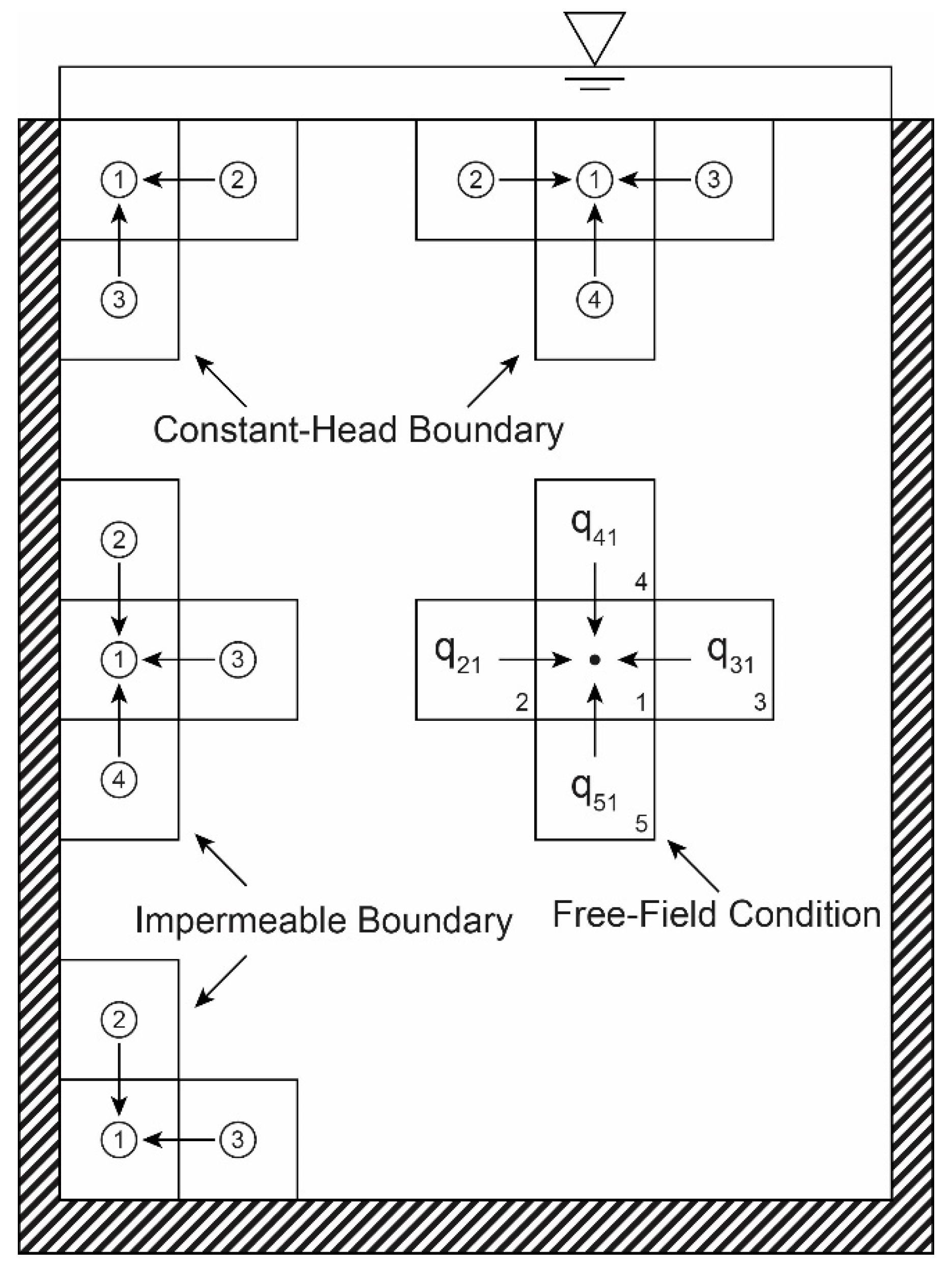
A finite element approximation of Darcy’s law was used to calculate the pressure distribution, velocity gradient, and the average flow rate for the BSF designs at each media condition. Each filter was divided into 1 cm by 1 cm cells, and the finite element approximation was calculated using a combination of constant head, free-field, and impermeable boundary conditions for each respective cell position throughout the filter. These boundary conditions are displayed in Figure 2 and are defined mathematically by Fox (1996) and Akhter (2006) using the finite difference method [35,36]. By splitting the effective area into M by N cells, each cell was assigned a unique value (e.g., pressure, velocity, the flow rate), where the entire effective area had independent equations following the present boundary conditions. The number of cells in the effective area thus depended on the length and width of each cell described in Equations (1) and (2):
where was the height of the effective area [l], was the width of the effective area [l], was the length of each cell [l], was the width of each cell [l], and and were the height and width count of the cell matrix [unitless]; the total number of cells is then .
Since the equations representing each cell were independent, we then set them into three matrices—the first with M × N columns and M × N rows, the second with one column and M × N rows, and the third with one column and M × N rows. Multiplying the first and second matrix yields the third matrix, defined in Equation (3):
where was the first (coefficient) matrix representing the fractional terms in front of the equations outlined by Fox (1996) and Akhter (2006), represented the second (e.g., pressure or head) matrix of each node throughout the filter, and represented the third (e.g., constant head) matrix at each point in the filter [35,36]. Given the known coefficient matrix, C, and the known constant matrix, P, solving for the unknown variable matrix, h, through a matrix solver yielded a matrix of unique values (e.g., head) at each cell. This relationship is outlined in Equation (4):
where was the fractional term for the first cell in the first equation, was the unique value (unknown) for the first cell, and was the constant value for the first cell (this term was only non-zero for cells with a constant boundary condition—it was zero for every other cell in the matrix). Solving this equation for the unknown matrix yielded values at each selected cell throughout the filter. A visual representation of the head matrix and its respective velocity gradient is shown in Figure A1. The velocity gradient was then obtained using Darcy’s law at each cell, as described in Equations (5) and (6):
where was the velocity in the x or y direction [l/t], was the hydraulic conductivity [l/t], and represented the head in the x and y directions, respectively [l]. The total velocity, , throughout the BSF was then the sum of each horizontal and vertical velocity at every cell throughout the filter (Equation (7)):
With gravity-driven flow, the driving pressure or head decreases as a function of time as water level in the reservoir declines. This in turn causes the flow rate to decrease exponentially. Using small, discrete time steps with linearization, the flow rate and volume discharged throughout the filter were obtained as a function of time [37], as outlined in Equations (8) and (9):
where [l3], [l/t], and [l] represent the volume discharged, filter velocity, and height of the water in the reservoir at the current time step, respectively, [l3], [l/t], and [l] represent the volume discharged, filter velocity, and height of the water in the reservoir at the next time step, represents the filter reservoir area [l2], and represents the time interval [t]. Using the finite element approximation of Darcy’s law at the current time step yielded velocity, which was then used to calculate the new driving pressure, and the new volume discharged, . For this study, we used 25 s time steps, ending at 5 h. Due to practical considerations for a 12 L reservoir volume, the model was capped at 5 h. To quantify the average velocity throughout the filter over the entire time interval, we assumed each configuration exhibited a behavior similar to exponential decay. The mean lifetime of an exponential decay function was calculated where the value of the function is reduced to 1/ of the function’s initial value. The average velocity was then approximated using Equation (10):
where was the average velocity for the entire time interval [l/t] and was the initial velocity throughout the filter [l/t] determined from the initial finite element approximation of Darcy’s Law. The average volumetric flow rate throughout the entire time interval follows Equation (11):
where is the average volumetric flow rate [l3/t]. The results for the average velocity for each filter design and media type were then used to analyze the percent removal of E. coli in the contaminant modeling experiments described in Section 2.5.
2.5. Contaminant Removal Modeling
In the BSF, sand particles act as a collector which attracts contaminants (e.g., bacteria and viruses) that act as colloidal particles experiencing interception, diffusion, and sedimentation forces [25,38]. As water filters through the sand bed, these particles are further removed by screening, adsorption, and natural death, resulting in an effluent supply of water with reduced bacterial and viral concentrations [20,25,27]. The log removal of microorganisms by attachment can be described using the colloid filtration equation of Yao et al. (1971; Equation (12)):
where was the concentration of microorganisms at the outlet [CFU/100 mL], was the concentration of microorganisms in the influent water [CFU/100 mL], was the porosity of the filtering media [unitless], was the grain size of the collector [l], was the media bed depth [l], was the sticking efficiency [unitless], and was the single collector efficiency [unitless] [25]. We then included the effect of the biolayer on contaminant removal using Equation (13) developed by Schijven et al. (2013):
where was the scale factor for the particle (microorganism) [m°C], was the temperature of the water [°C], was the rate coefficient [t−1], and was the age of the biolayer [t] [20]. The single collector efficiency (η) was calculated using the colloid filtration theory equations developed by Tufenkji and Elimelech (2004) [38]. The fluid viscosity () of water [kg/m°C] was assumed to be temperature dependent and was calculated using Equation (14) [39].
The sticking efficiency (), introduced by Vissink (2016), was first quantified using Equation (15):
where was a sticking factor [], was the power of the grain size [unitless], and was the power of the velocity [unitless] [27]. While this correlation is statistically accurate for filtration systems with velocities greater than 0.3 m/h, this model breaks down for systems at very small velocities. At filter velocities lower than 0.3 m/h, this correlation reports values for the sticking efficiency that are greater than one, violating the restriction that the sticking efficiency must be less than or equal to unity and resulting in an overestimated contaminant removal value. The current model also relates a larger sticking efficiency and percent removal with increase in grain size, which goes against much of the background research on slow-sand and biosand filtration systems [7,21,22].
The contaminant removal model introduced in this paper mirrors that introduced by Vissink but accounts for systems which exhibit very low Darcy velocities, such as the BSF. The model was based on an exponential decay function and agrees with the previous model at a Darcy velocity of 0.4 m/h for the grain size of 0.5 mm using the constants outlined in Vissink (2016) [27]. The velocity of 0.4 m/h and grain size of 0.5 mm represent average filtration velocities for biosand and slow-sand filtration (0.1–0.4 m/h; [28]) as well as a common grain size for both filtration techniques (medium–coarse sand). We then quantified the sticking efficiency using Equation (16):
where was an exponent [unitless] and was a new sticking factor []. Both factors were determined from correlation with the current model developed by Vissink (2016) and from previously reported values from Schijven et al. (2013) [20,27]. Data for the sticking and the single collector efficiency in the control filter at varying grain sizes are found in Figure A2 and Figure A3. Selected values used to calculate the sticking efficiency, the single collector efficiency, and the log removal of E. coli and MS2 for each experimental trial are summarized in Table A1. Values for the particle density, particle diameter, Hamaker constant, porosity, scale factor, and rate coefficients were synthesized from an extensive literature search. For each experimental trial, the fluid temperature was kept constant at 25 °C, porosity at 42%, and the age of the biolayer at 14 days. E. coli was selected for its pathogenic properties and widespread use as a reference for contaminant removal in slow-sand filters. Although several other strains of pathogenic bacteria cause severe illnesses and waterborne diseases such as cholera, typhoid fever, and gastroenteritis, these bacteria are harder to isolate and culture and therefore the use of indicator bacteria is required [40]; E. coli is frequently used as a broad bacteria proxy due to its large presence in human and animal intestines [40]. MS2 was chosen because of its reputation as a conservative model virus [41].
3. Results
3.1. Fluid Velocity and Discharge
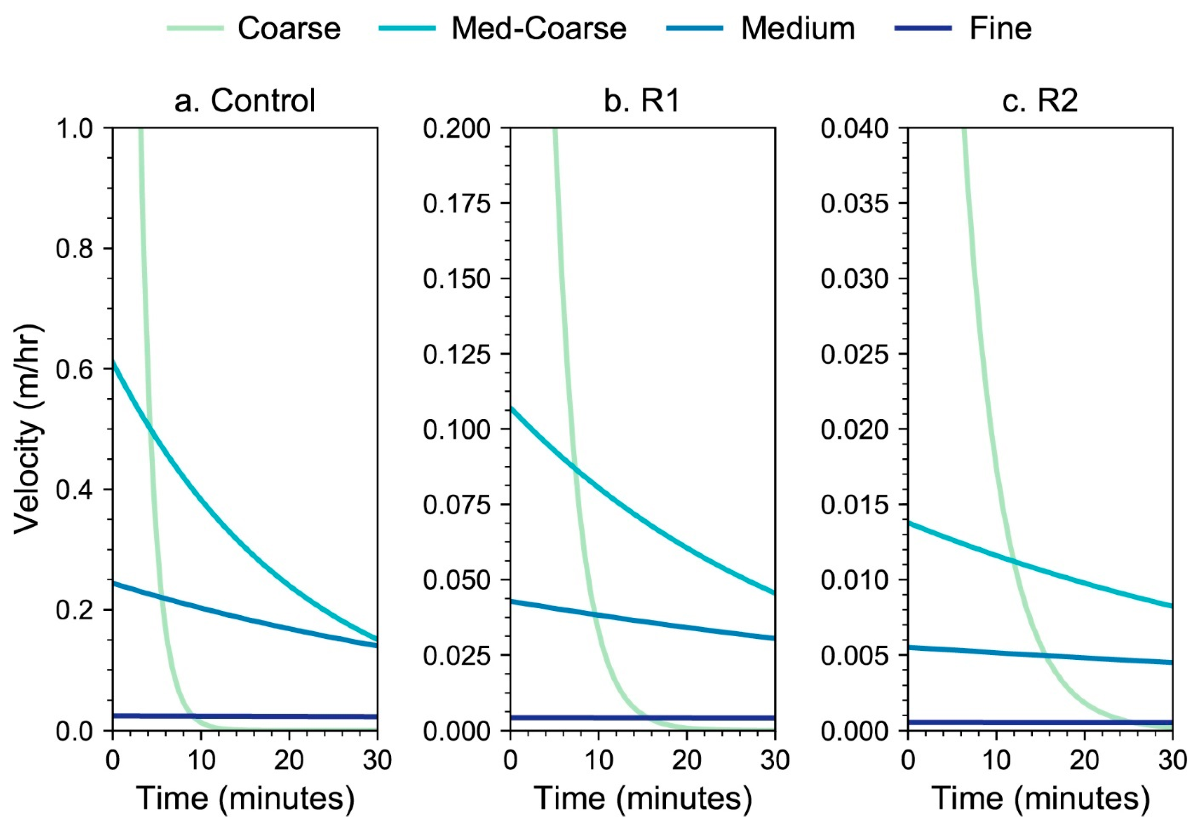
Results of the finite element approximation of Darcy’s Law modeling (Section 2.4) for fluid velocity through each BSF design and media condition are displayed in Figure 3.
Each filter velocity displayed trends similar to exponential decay. R2 (Figure 3b) and fine sand displayed the lowest velocities of each filter and filter media, respectively, while the control filter (Figure 3a) and coarse sand displayed the highest velocities of the three filters and four media types. Filter designs using coarse sand experienced much larger slopes with high initial filter velocities, while designs using fine sand displayed very gradual slopes with low initial filter velocities. For coarse sand, the initial velocity was 7.32 m/h for the control, 1.28 m/h for R1, and 0.17 m/h for R2. For fine sand, the initial velocity was 0.0244 m/h for the control, 0.0043 m/h for R1, and 0.0005 m/h for R2. The initial velocity directly impacts the average filter velocity from Equation (10), resulting in average velocities for R2 being lower than R1 and the control. The average velocities for each design with varying media are displayed in Table 3.
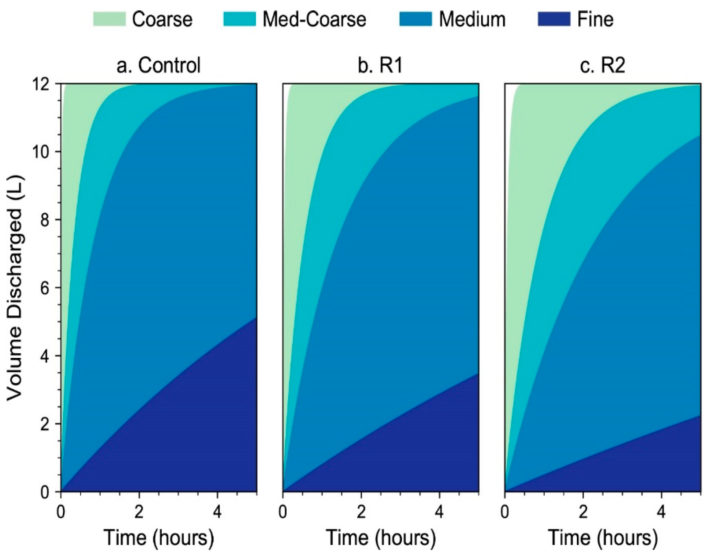
Following the same pattern as the initial velocity, the average velocity for each filter design and media used decreases from the control to R2 and from coarse to fine sand, respectively. As the media decreases in hydraulic conductivity, the average filter velocity decreases with the lowest value evident in R2 with fine sand as the filtering media. Average filter velocities varied from 2.6933 to 0.0002 m/h with the lowest flow rates corresponding to finer media and decreased filter height. For the control, the average velocity is consistently approximately forty-four times as large as R2 and approximately six times as large as R1. The average velocity using coarse sand is approximately three hundred times as large as the velocity using fine sand. While there is a large discrepancy in average velocity values between filter designs and media, the differences between the volumetric flow rate and volume discharged for each design and media are closer together on average. Results for modeled discharge are displayed in Figure 4 and exhibit similar values and trends between filter designs and media.
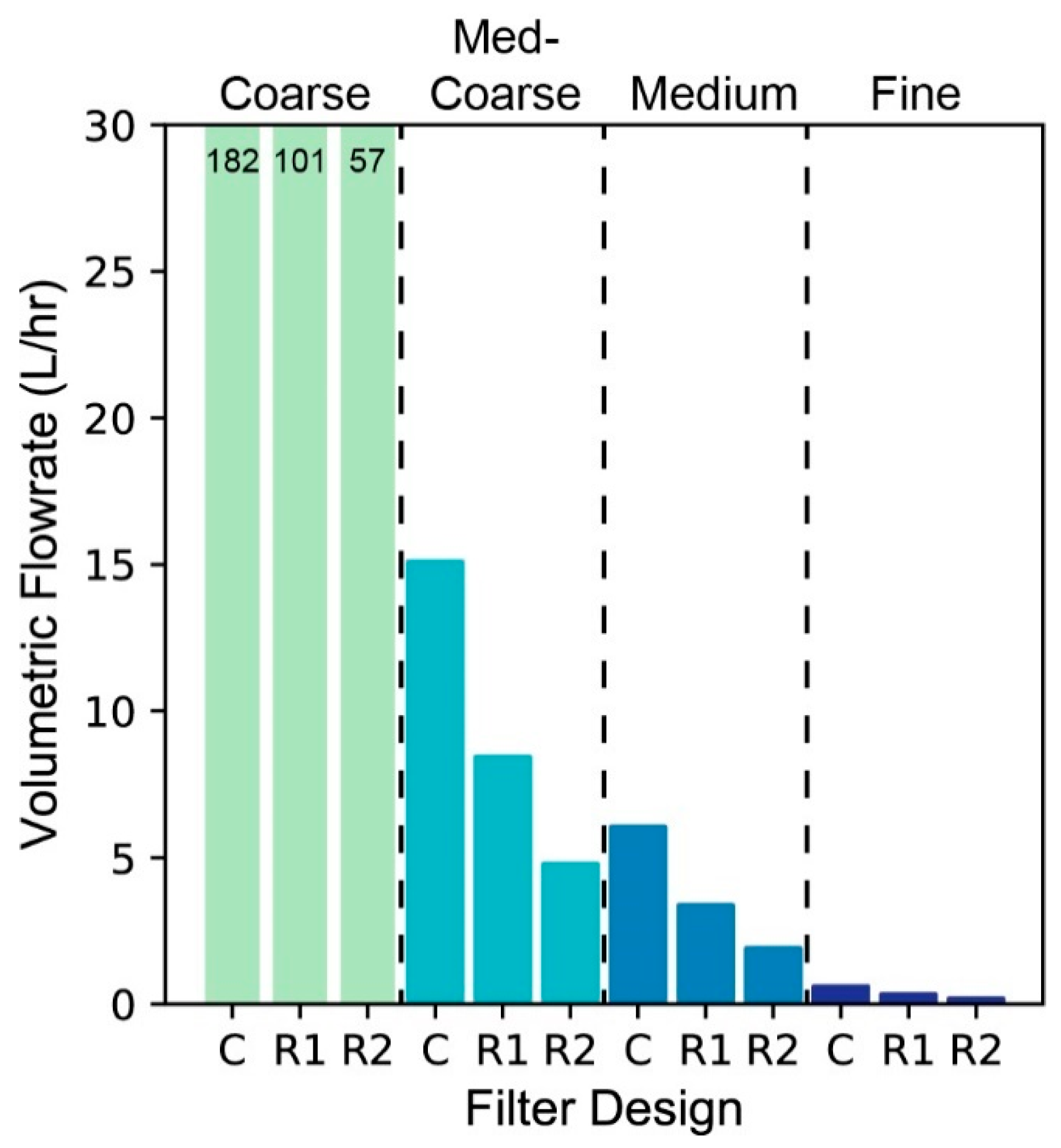
Figure 4a–c all show the same trend, with a color fill between media to allow for a ranged estimate of the percent removal per sand type: as time increases, the volume discharged increases, but with different rates between media types. For the control filter, coarse sand exhibited full discharge (12 L) in just 15 min, medium–coarse sand in 2 h, medium sand in 4.5 h, while fine sand was incapable of full volume discharge within the 5 h interval. For R1, coarse sand exhibited full discharge in approximately 20 min, medium–coarse sand in approximately 3 h, and medium and fine sand were incapable of full reservoir discharge. For R2, coarse sand exhibited full discharge in approximately 30 min, medium–coarse sand in approximately 5 h, and medium and fine sand were still incapable of full volume discharge. Because of a high initial velocity, filter designs using coarse sand experience much higher flow rates and are therefore more capable of filtering the full reservoir in less time. Much like in Figure 3, filter designs using coarse sand have much larger slopes than designs using fine sand. This results in a higher average volumetric flow rate for the control and coarser media. These average volumetric flow rates varied from 181.5 to 0.19 L/h, as shown in Figure 5.
Figure 5 also shows that as the filter design moves toward a reduced height, the volumetric flow rate decreases. In addition, the overall trend is that the average volumetric flow rate decreases between filters as the hydraulic conductivity decreases. For fine sand, the volumetric flow rates are 0.61, 0.34, and 0.19 L/h for the control, R1, and R2, respectively. For coarse sand, these values are approximately 300× greater, at 182, 101, and 57 L/h for the control, R1, and R2, respectively.
3.2. Contaminant Removal
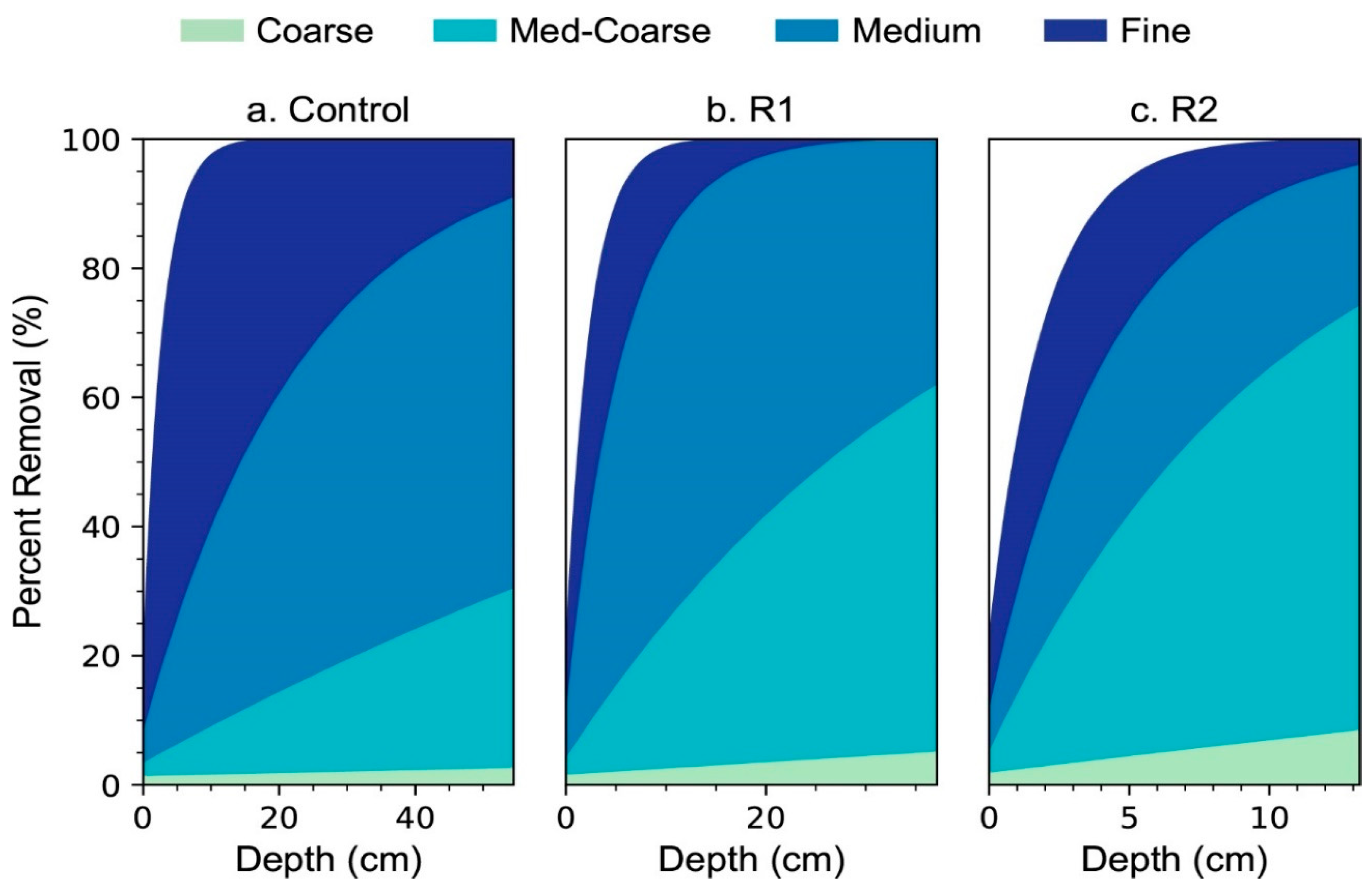
Results of the contaminant removal modeling (Section 2.5) for E. coli for each BSF design and media condition are displayed in Figure 6.
Using the average filter velocities calculated from the fluid modeling trials, the average contaminant removal of E. coli was determined at various depths throughout each filter design with varying media. Figure 6a–c represent the percent removal of E. coli versus depth, with a color fill between media to allow for ranged estimates of percent removal for each sand type. R2 exhibits the highest percent removal, with medium sand displaying near complete contaminant removal by just the first centimeter of the sand bed. Each filter using fine sand has near 100% (1.89 log control, 2.51 log R1, and 3.40 log R2) removal by contact with the effective area (0 cm), due to the chemical and biological removal interactions within the biolayer. Using coarse sand, each filter design was incapable of producing a satisfactory removal of E. coli at full depth with only 16.1% removal from the control, 23.5% removal from R1, and 35.7% removal from R2. As grain size decreases, the percent removal for each filter increases, with the largest variations in contaminant removal evident between the coarse and medium–coarse sand grains.
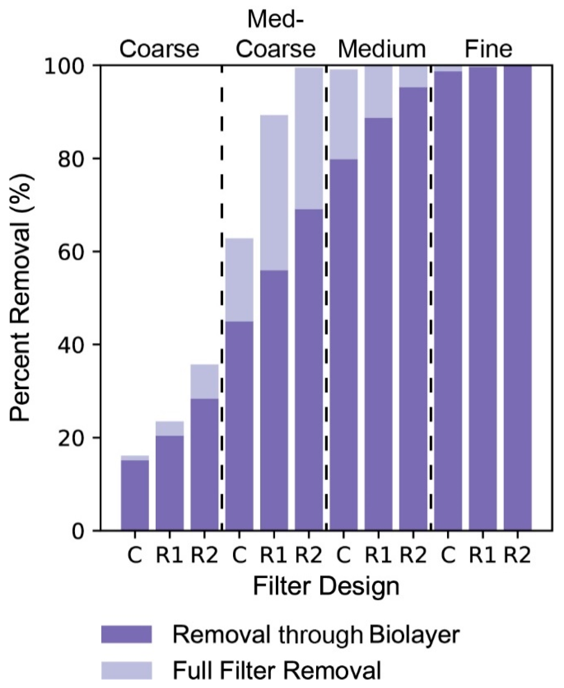
Figure 7 shows the percent removal for each filter design and media at the surface of the effective area (z = 0, after contact with the biolayer) and at the full filter length (z = L). Removal through the biolayer increases steadily as the filter design moves toward a reduced height and the media decreases in grain size. Removal of E. coli is greatest with R2 at all sand sizes and has the greatest removal with the smallest grain sizes. With fine sand, the effect of filter design and sand bed depth is more negligible, with nearly 100% removal from just the biolayer for all designs. At full filter depth, R2 had near 100% (>6 log) removal with medium–coarse, medium, and fine sand. R1 had near 100% (>6 log) removal with both medium and fine sand. The control only had near 100% (>6 log) removal with fine sand, with 99.58% (2.38 log) removal with medium sand.
Results of the contaminant removal modeling (Section 2.5) for MS2 for each BSF design and media condition are displayed in Figure 8.
The percent removal of MS2 versus depth (Figure 8) displays the same trends as Figure 6 for E. coli; as the depth increases, the percent removal of contaminants increases. While both Figure 8 and Figure 6 display the same trends, it is apparent that the removal of MS2 is less, comparatively, and shows a greater variation as the sand bed depth increases. Between filters, R2 generally had a greater percent removal of MS2 than the control and R1, with fine sand having the greatest removal of the medias used. Coarse sand did not have adequate removal rates at any design with a 2.30%, 4.54%, and 7.56% removal at the control, R1, and R2, respectively. Fine sand had the greatest effect with near 100% (>6 log) removal of MS2 for each filter design used.
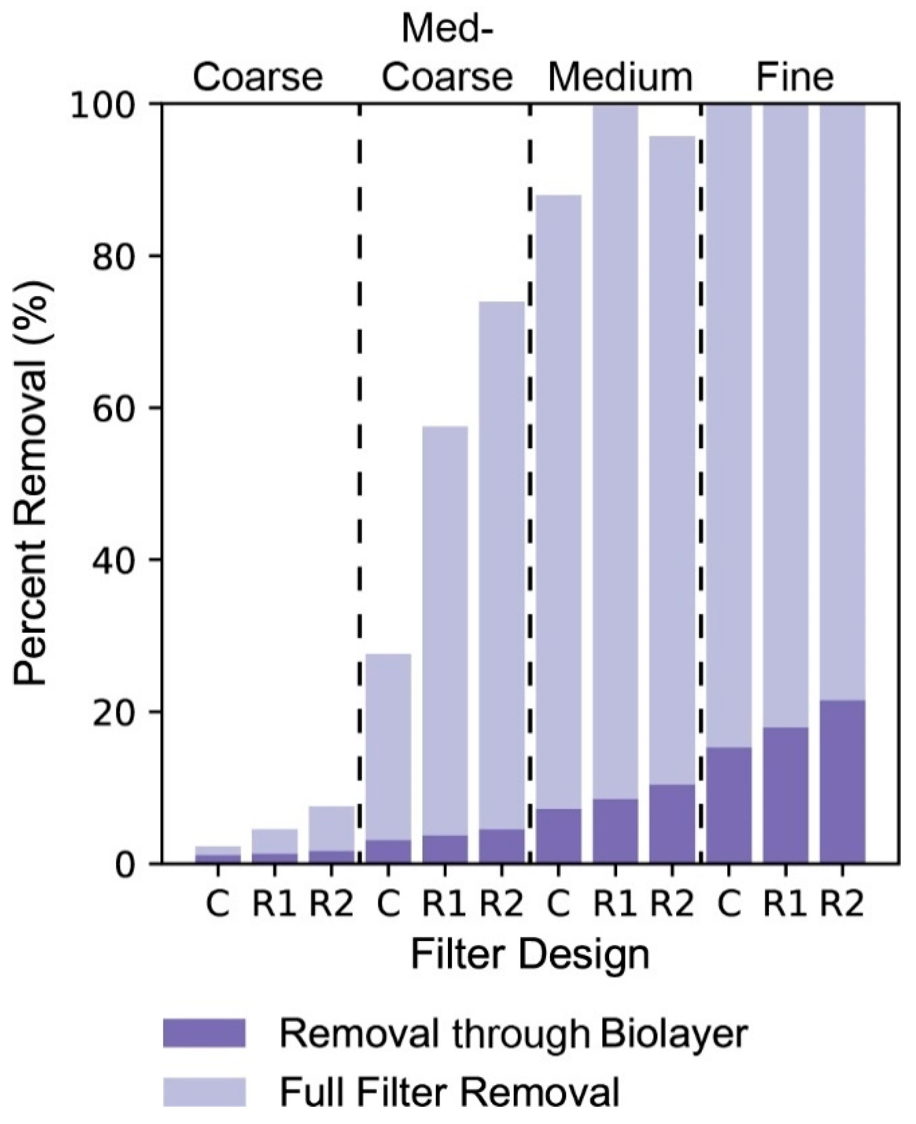
Figure 9 shows the percent removal for each filter design and media at the biolayer (z = 0) and at the full filter length (z = L). From Figure 10, the percent removal of MS2 displayed the same overall trends as that of E. coli with respect to the sand bed depth, filter design, and media used, but the values for the removal efficiency were comparatively less. For the control at the full filter length, only fine sand was able to achieve effectively 100% (>6 log) removal of the MS2 virus while medium sand displayed an 88.0% removal, medium–coarse sand a 27.6% removal, and coarse sand a 2.3% removal. Although at fine sand, each filter design was able to achieve 99.9% (3 log) removal of MS2, only R1 was able to achieve a 99.7% (2.52 log) removal at medium sand.
Figure 8 and Figure 9 demonstrate that the biolayer had very little impact on the removal of MS2, while the sand bed had a very large contribution. For R2 using medium–coarse sand, removal from the biolayer was 4.6%, while the removal at the full filter length was 99.7%. This large difference between the removal at the biolayer and the full filter length is very evident for R1 and R2 at medium–coarse, medium, and fine sands, but less evident for coarse sand and the control. Although for coarse and medium–coarse sand, R2 had a greater percent removal of MS2 than the other two filters, R1 outperformed the control and R2 at medium and fine sand. At medium sand, the removal efficiency of R1 is 99.7%, while it is 95.8% (1.38 log) for R2. At fine sand, the difference is smaller, but still noticeable, with a 99.99% (4 log) efficiency for R1 and a 99.91% (3.05 log) efficiency for R2.
4. Discussion
4.1. Comparison Between Designs
Contaminant modeling indicated that the R1 and R2 designs reduced a greater quantity of bacteria and viruses from a contaminated supply compared to the control design at all media sizes. This improved removal in R1 and R2 is due to (1) a reduced reservoir height, (2) slower fluid velocity, and (3) increased biolayer area.
The reservoir height is an important metric to the gravity-driven design, as filter pressure head (i.e., the height difference between the water level in the reservoir area and the outlet) directly affects the velocity of the filter and ultimately the residence time (or contact time) of contaminated water with the biolayer and effective area at each media size. In this study, R2 had the lowest pressure head and subsequently the lowest flow velocities. This allowed for the greatest contact time with the biolayer and effective area, ultimately allowing for improved contaminant removal. Here, flow velocities in the control were more than three-fold greater than those in R2 for each media type. Mathematically, slower velocities allow for increased sticking efficiency and single collector efficiency (Equation (16); [38]), and velocity and contaminant removal are inversely related (Equation (13)). However, slow velocities can also lead to impractical volumetric discharge (i.e., not enough clean water is discharged from the filter for reasonable use).
Total filter discharge for each media type is a function of velocity (i.e., pressure head) and the volume of dirty water supplied to the filter per use. If the pressure head were to be reduced in the control to match R2, the total volume of dirty water supplied to the control would be minimal, drastically reducing the total discharge of the filter. However, the R2 design has a much greater surface area than the control, so a reduced head does not equally hinder total filter discharge (i.e., minimal water over a large area can still result in high discharge compared to much water over a small area). Here, R1 and R2 both have less total discharge than the control, so these designs would need to be made wider, the total reservoir volume increased, or uses more frequent to match the control.
A wider filter design such as R1 or R2 also allows for a greater biolayer area, and subsequently greater contaminant removal, particularly for bacteria (Figure 7), when compared to the control. As for viruses, removal is mostly a function of contact time with the effective area and less the biolayer, as evidenced by R1 outperforming R2 at medium and fine sands (Figure 9). In the control design, the filter must be made tall to accommodate higher velocities (i.e., greater pressure head) and shorter contact times. In R1 and R2, velocity is reduced and contact time increased due to smaller pressure heads, so the total filter height can also be reduced without compromising virus degradation. However, R2 is near its minimum height to achieve 100% (>6 log) removal for both E. coli and MS2 at finer sands (Figure 6, Figure 7, Figure 8 and Figure 9).
In addition to the reservoir height, velocity, discharge, contaminant removal, and contact time are also a function of the media size (coarse, medium–coarse, medium, fine). Here, the finer the grain size, the lower the velocity and discharge and the higher the contaminant removal and contact time. For example, coarse sand in R2 removed only 35.74% of E. coli, where medium–coarse sand removed 99.50% (2.30 log). Yet, medium–coarse sand only removed 73.96% of MS2, where fine sand removed near 100% (>6 log) of E. coli and 99.91% of MS2. Fine sands may prove effective but impractical due to limited discharge; successful application of BSF technology requires a balance of practicality and performance (most are constructed using medium sand with an effective diameter of 0.15–0.35 mm; [28]). Under medium sand conditions, both R1 and R2 outperformed the control when focused on a balance of practical discharge and successful contaminant removal.
4.2. Biolayer Age and Media Depth
Physical testing has shown that contaminant removal can increase with a mature biolayer (i.e., removal becomes greater over time) [8,20]. While we kept a constant biolayer age (14 days), Equation (13) calculates greater contaminant removal with older biolayer age values. This is most relevant for bacterial contaminants (e.g., E. coli), as they are largely removed across the biolayer compared to viruses (Figure 8 and Figure 9). However, viruses are instead deactivated by longer residence times in the effective area and are less impacted by the biolayer [42]. While it may be possible to achieve effectively 100% bacterial removal with just the biolayer, viruses likely require additional media depth at the BSF scale. Thus, there are limiting factors to contaminant removal, as bacteria may be constrained by biolayer maturation and viruses by media depth relative to the fluid velocity and subsequent residence time in the filter. The methods applied here can quantify the minimum values for future design purposes.
4.3. Literature Agreement
Table 4 displays our modeled results for E. coli removal relative to previous physical testing from other experiments found in literature searches. Literature values from previous lab or field studies are shown in column 2, model results obtained from this study are shown under the respective sand grains in columns 3 and 4, and the percent difference between previous studies and our model results are displayed in column 5.
For both fine and medium sand, our model results were supported by physical testing from literature. The greatest difference between our modeled results and physical results was at 0 cm depth (i.e., surface of the effective area). This is likely due to variance in modeled versus actual grain sizes. The literature value reported is also for continuous operation, which may impact the development and full removal capacity of the biolayer with intermittent operations (note all other literature values are with intermittent use). All other values for fine sand were within 1% of the observed removal, and coarse sand was within 2%. Even for MS2, modeled removal agreed with results found from Elliott et al. (2008), Schijven et al. (2013) and Vissink (2016) [8,20,27]. Variance between the modeled and reported values from previous studies may be further due to one or more of four reasons: (1) the constants outlined in Table A1 could vary between physical experiments and different filters, (2) experimental conditions (temperature, fluid velocity, grain size, and biolayer age) could differ based on climate and experiments, (3) results between intermittent and continuous filter operation could differ, and (4) inherent errors within the slow-sand filtration model (±0.6 log) could overestimate the percent removal of contaminants. Despite these discrepancies, the slow-sand filtration model, as used in this study, provided near complete agreement and is a robust method for estimating contaminant removal for the BSF. Although not previously discussed and not modeled in this paper, a summary of heavy metal contaminant removal throughout the BSF can be found in Appendix E: Heavy Metals.
4.4. Comparison to Ceramic Filtration
Overall, the R1 and R2 designs are more effective at removing E. coli and MS2 than the traditional BSF for each media type, but their discharge rates are slower and more in line with ceramic filters at finer media sizes (another common HWT solution). Using medium sand, R2 is able to remove effectively 100% (>6 log) of E. coli and 95.75% of MS2 from the influent water supply and produces an average of 1.912 L/hr which falls within the existing flow rates for ceramic filtration. R1 removes near 100% (>6 log) of E. coli and 99.71% of MS2, while producing an average of 3.380 L/hr. Using medium–coarse sand, the R2 design removed 99.50% of E. coli and 73.96% of MS2, while producing an average of 4.781 L/h, lower than the traditional CAWST v.10 BSF but higher than most ceramic filters (R1 was 89.32% for E. coli, 57.51% for MS2, and 8.440 L/hr). Whereas ceramic filters are capable of the same removal efficiency of E. coli as the R1 and R2 designs, they do not have the same efficacy when it comes to the removal of MS2 [15]. As a result, the R1 and R2 design effectively outperform ceramic filters in their overall removal efficiency while offering a higher flow rate.
4.5. Model Limitations and Experimental Error
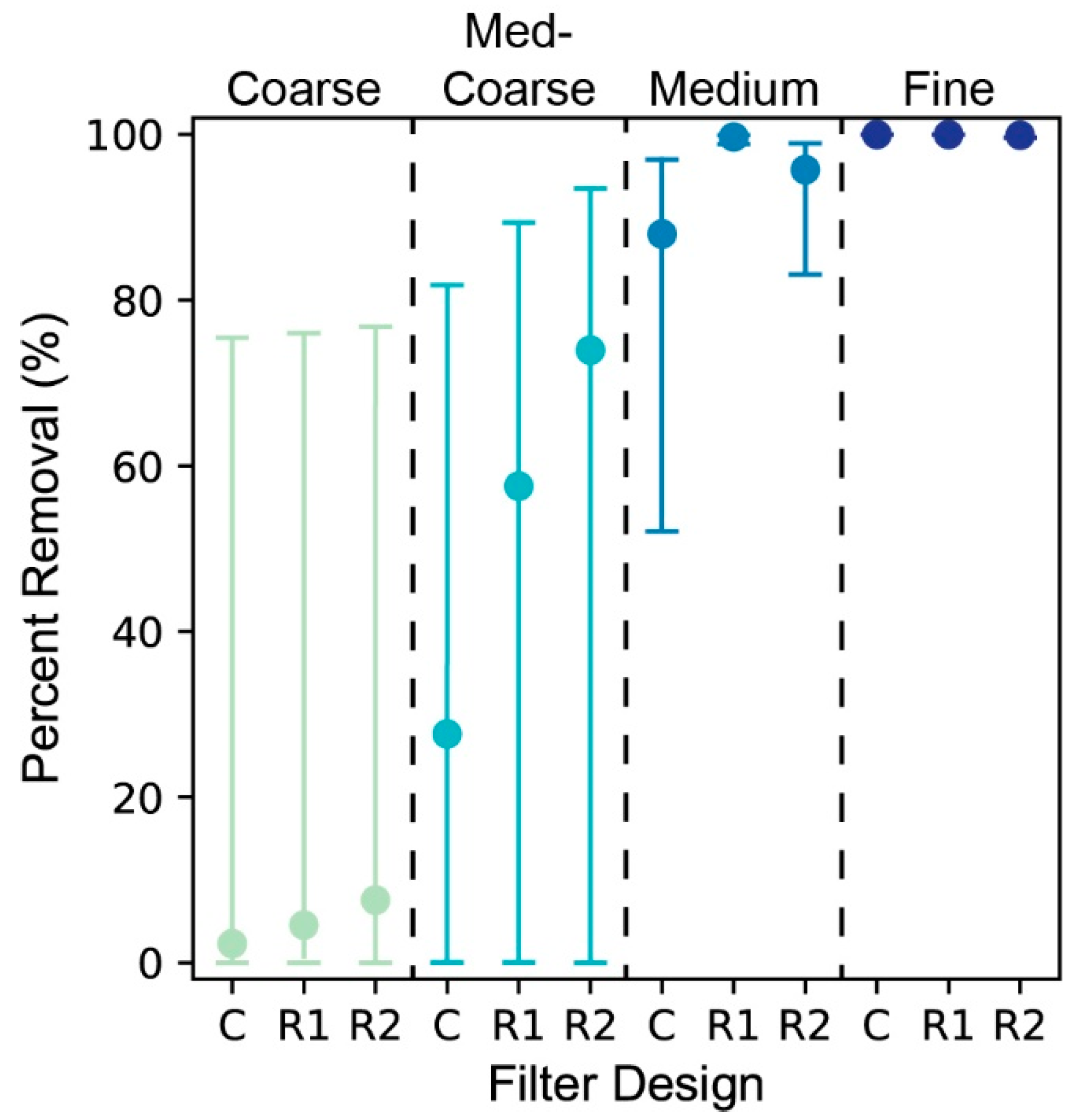
Given Equation (13), this study estimates removal of E. coli and MS2 within ±0.6 log, as derived from Schijven et al. (2013) [20]. Error bar plots of the percent removal versus filter design and filtering media for E. coli and MS2 are shown in Figure 10 and Figure A4, respectively.
Estimates at finer media and reduced filter height (R1 and R2) have the smallest error ranges. This is from the high log and percent removal experienced from these conditions. Because of the relationship between log and percent removal, at high enough log removal values (usually greater than 3 log), a ±0.6 log error will not significantly alter the percent removal. Due to the difference in models for the sticking efficiency, this experimental error is likely to vary between physical studies but should overall be close to the value reported by Schijven et al. (2013) [20]. Furthermore, this study uses more conservative values as inputs into the slow-sand filtration model, resulting in more conservative estimates for the percent removal of contaminants within the slow-sand filtration model. Despite any further discrepancies or potential errors, the conservative values used as inputs for the model should indicate values for the percent removal close to more conservative estimates.
4.6. Practical Design Applications
Maximizing the bioactivity area (i.e., active contaminant removal), increasing the residence time inside the filter (i.e., passive contaminant removal), and reducing the overall height of the design has several practical design applications that open pathways for new construction technologies and multifamily designs. For example, a reduced-height design lowers the lateral load (i.e., pressure) imposed on the walls of the filter due to less sand bed depth and the directly proportional relationship between lateral load and depth of sand or water. Both these benefits can allow for the introduction of concrete alternatives that may not meet industrial (i.e., strength bearing) standards but are still suitable for BSF applications, such as cement made out of wood ash, instead of or mixed with industrial concrete mix, which could further allow for construction with on-site materials (e.g., biomass) [43]. Furthermore, the horizontal designs outlined here mimic the benefits observed in natural wetland environments (e.g., long residence times, biofiltration; [44]), which indicates potential for upscaling the size of a BSF to a communal scale [45]. A large, broad BSF could feasibly provide clean water to several families while also overcoming the reduced flow rates observed in the single-family design modeled here when compared to the traditional BSF design (i.e., filter discharge volumes with slow flow-rates across large areas can be greater than fast flow-rates across small volumes). In terms of single household or personal use, the flow rates of a reduced-height design will prove slower compared to the traditional design of the same media. This does not render the reduced height impractical, as its flow rates are still on par with other popular filtration solutions (i.e., ceramic filters), but it may require an instructional shift (i.e., users may need to prepare earlier in advance for when water may be needed). The reduced-height design also requires an increase in width to maintain removal rates, meaning the surface area required within a home (i.e., interior footprint) will increase. The practicality of increased interior space dedicated to a filter is site dependent; an outdoor, communal, or multifamily filter design may be suggested in scenarios with limited space.
5. Conclusions
The BSF is a robust and successful HWT solution for undeveloped or developing regions with contaminated water supplies, but its function can be improved and its application more widespread through design modifications that prioritize efficient use of filter space, scalable sizes that can serve larger households, and materials that allow for distribution in remote areas of the world. The purpose of this study was to model both the hydraulic patterns and contaminant removal inside three BSF designs to evaluate how these dynamics change with varying filter shapes. Specifically, we sought to prioritize the valuable function of the biolayer while eliminating inefficient space found in the traditional BSF design. We used a combination of finite element approximation of Darcy’s law with discrete time steps and slow-sand filter contaminant modeling to analyze both the fluid flow and filter performance at removing the E. coli bacteria and MS2 virus. From the results of this study, we can conclude:
- Slower fluid velocities through the filter require less effective area depth, as residence times inside the filter increase. Increased residence times allow for longer contact time with the both the biolayer and effective media which leads to greater bacteria removal and virus deactivation. For the BSF, slow velocities are directly related to the hydraulic conductivity of the effective media, where fine sands have the greatest reduction in fluid velocity. Thus, BSF designs with finer-grained media can be designed with shorter filter bodies relative to the traditional BSF design size. Reduced velocities can also be achieved through decreased head pressure, which can be obtained by a shorter standing height on top of the filter media with each use. To maintain the total volume of discharged water, reduced standing heights require a wider filter body than the traditional design.
- Increased biolayer area leads to greater contaminant removal. Particularly for bacteria, contact with the biolayer is the most notable filtering mechanism in the BSF. Designs which increase the biolayer area relative to the traditional BSF design will have greater contaminant removal rates, assuming other conditions are consistent between filters. This can be accomplished through a wider design, which also enables a reduced standing water height above the filter media and slower fluid velocity as outlined in Conclusion #1. Under the proper conditions, BSF technology can remove nearly all bacteria contaminants through just the biolayer.
- Viruses, unlike bacteria, are less impacted by the biolayer and are more effectively removed with longer residence times inside the BSF. Longer residence times can be achieved by decreased media grain size (i.e., hydraulic conductivity), taller effective areas (i.e., taller filter bodies), or slower fluid velocity (i.e., slower water flow). With a modified design, BSF technology can remove 100% of virus contaminants.
- The R1 and R2 designs outperformed the traditional BSF in contaminant removal at all media grain sizes, but their total discharge was notably less. While not outside of other common HWT solutions at fine grain sizes, the discharge rates of R1 and R2 can be improved by a larger filter surface area or larger media grain sizes. With sand characteristics commonly used in the traditional BSF, both the R1 and R2 designs outperformed the traditional design while also maintaining practical discharge rates.
Collectively, the results of this study highlight how a modified design can improve the overall performance of BSF technology. This is particularly relevant for alternative construction methods which may be capable of building short and wide filters rather than tall and narrow bodies such as the traditional BSF (e.g., single cast designs without a mold or concrete mix). As a result, the modified design can (1) reduce the weight of required BSF materials while (2) extending distribution to remote areas of the world not easily accessible by common transportation methods. Thus, modified BSF designs that focus on efficient removal and simple construction methods can improve the overall impact of providing clean water to the 10% of the world’s population that still lacks access to clean and reliable water supplies [1].
Author Contributions
J.A.P. developed the model and completed the analysis with supervision from S.J.S. Writing and figures were collaborative efforts. All authors have read and agreed to the published version of the manuscript.
Funding
This work was partially funded by the University of Florida, Institute of Food and Agricultural Sciences. P.I. Smidt’s lab funded the project.
Acknowledgments
A special thanks to the members of the Land and Water Lab and the Soil and Water Sciences Department, University of Florida/IFAS, Gainesville, Florida.
Conflicts of Interest
The authors declare no conflict of interest.
Appendix A. Pressure Distribution
The average pressure distribution and velocity gradient for the control filter from the fluid modeling results are shown in Figure A1. The head pressure at each cell moving downward through the filter is less than at the beginning of the filter, due to the high pressure of the reservoir and low pressure of the outlet. Because of greater differences in head pressure between cells at the bottom of the sand bed, the velocity gradient at the bottom of the filter is larger than at the top. While for the actual fluid modeling experiments, the length and width of each cell was equal to 1 cm, for this figure, the dimensions of each cell were 3 cm by 3 cm. This was to easily portray the velocity gradient throughout the filter.
Figure A1.
Pressure distribution and velocity gradient through sand bed of the filter control.

Appendix B. Collector and Sticking Efficiency
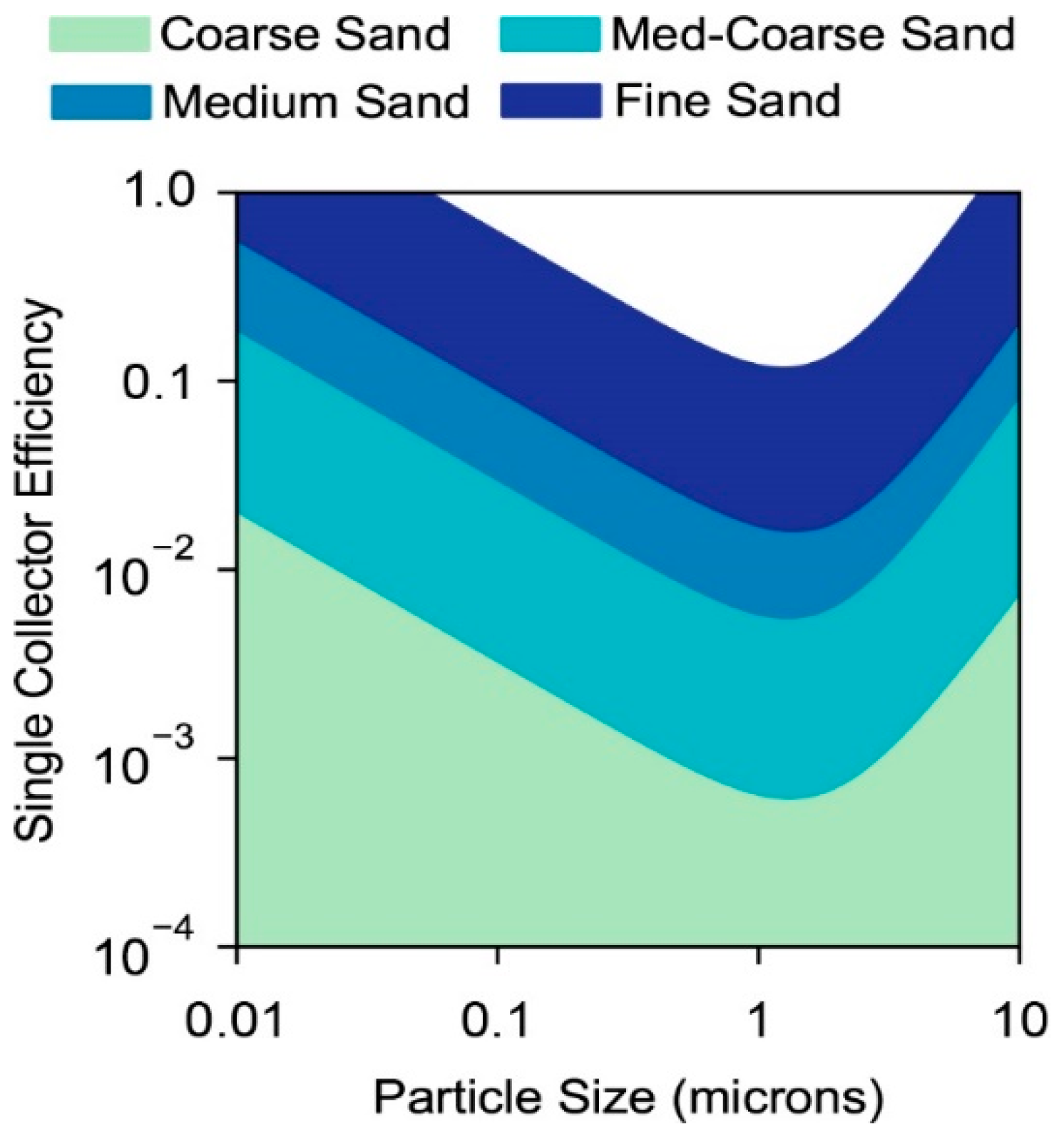
For the contaminant modeling experiments, the single collector efficiency was calculated by Tufenkji and Elimelech (2004) and verified by Yao et al. (1971) [25,38]. The results for this parameter for the control filter are shown in Figure A2. This figure shows a decrease in the efficiency due to diffusion forces as the particle size increases, then experiences a minimum efficiency approximately 1 micron, and then increases due to interception and sedimentation forces. As the particle size increases from 0.001 microns to 1 micron, the diffusion forces decrease from an increased aspect ratio between the particle (bacteria) and collector (sand). Above 1 micron, increases in gravitational contributions from larger particle sizes result in an increase in the collector efficiency. Using coarse sand, the single collector efficiency is much lower than that for fine sand, with medium and medium–coarse sand in between these two.
Figure A2.
Single collector efficiency versus particle size for the control design with varying media.
Figure A2.
Single collector efficiency versus particle size for the control design with varying media.

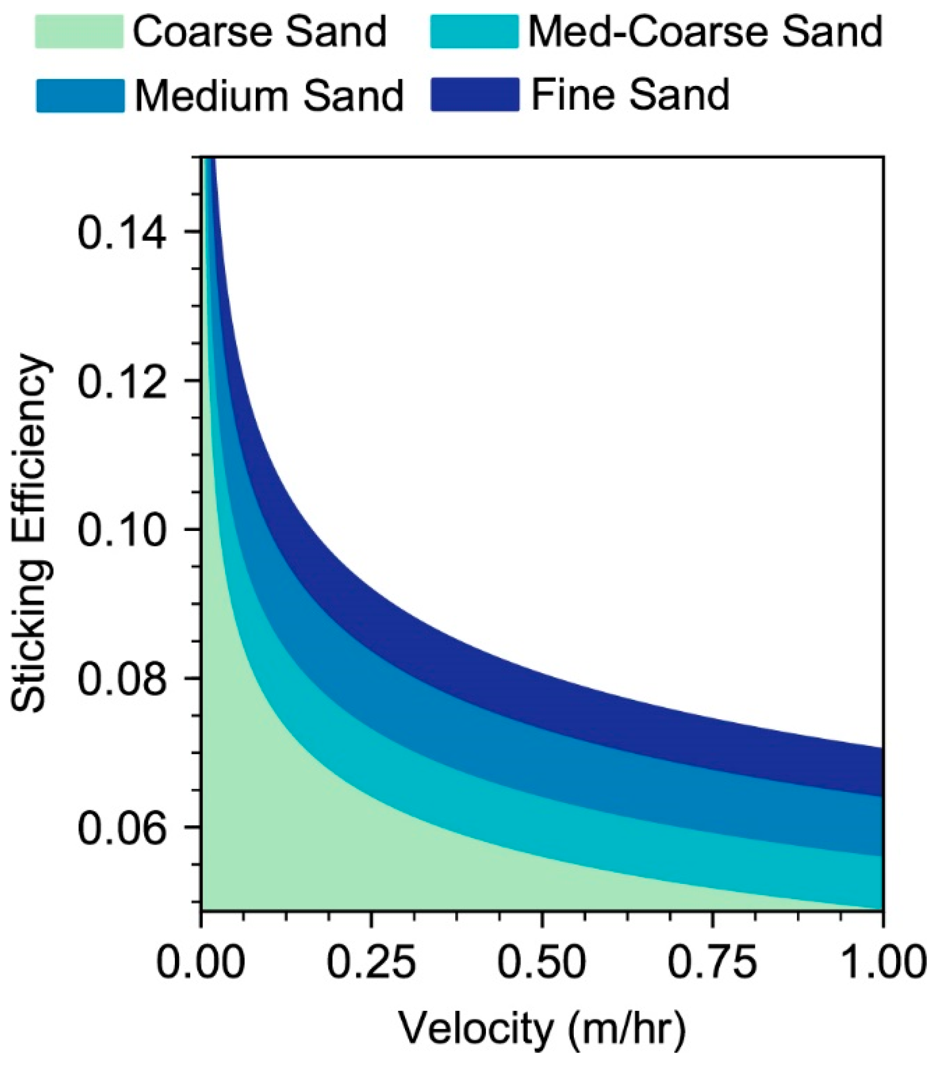
The sticking efficiency for the control filter in the contaminant modeling experiments is shown in Figure A3. As the velocity increases, from Equation (16), the sticking efficiency decreases, with the smallest values evident at very low filtration velocities. As the velocity decreases, this allows for a greater residence time throughout the biolayer and effective area, leading to more bacteria and viruses being removed from the influent water supply. The greater the time spent throughout the filter, the more bacteria and viruses will collect to the surface of the sand grains and other bacteria in the biolayer. At fine grain sizes, the sticking efficiency displays the greatest values while at coarse sand, this efficiency is greatly reduced.
Figure A3.
Sticking efficiency versus velocity for control at varying media.

Appendix C. Model Constants
The constants and variables used to calculate the single collector and sticking efficiencies for the contaminant modeling experiments are shown in Table A1.

Table A1.
Description and values of variables and constants.
| Constant | Constant Description | Value | Units |
|---|---|---|---|
| Particle Density (E. coli) 1 | 1160 | kg/m3 | |
| Particle Density (MS2) * | 1000 | kg/m3 | |
| Particle Diameter (E. coli) | 1 | μm | |
| Particle Diameter (MS2) | 27.5 | nm | |
| Gravitational Constant | 9.80 | m/s2 | |
| Boltzmann Constant | 1.38 × 10⁻²³ | J/K | |
| Hamaker Constant 2 | 2.15 × 10⁻²⁰ | J | |
| Porosity 3 | 0.42 | - | |
| Fluid Density | 1000 | kg/m3 | |
| Power (E. coli) | 0.2 | - | |
| Power (MS2) | 0.1 | - | |
| a | Biolayer Age | 14 | days |
| Scale Factor 4,5 | 1.9 × 10⁻⁴ | m°C | |
| Rate Coefficient 4,5 | 0.072 | day−1 | |
| Sticking Factor (E. coli) | 0.0029 | - | |
| Sticking Factor (MS2) | 0.00075 | - |
These values were found from extensive literature searches and used to calculate the single collector and the sticking efficiency to be input into the slow-sand filtration model (Equation (13)). Table A2 displays these values for E. coli and MS2. The single collector and sticking efficiencies were calculated using the average filter velocities displayed in Table 3 and the grain size of the media displayed in Table 2.
Table A2.
Results for the sticking and the single collector efficiency for a traditional BSF design (C), a 40% reduced-height design (R1), and a 70% reduced-height design (R2).
Table A2.
Results for the sticking and the single collector efficiency for a traditional BSF design (C), a 40% reduced-height design (R1), and a 70% reduced-height design (R2).
| Type of Sand | Filter Design | Sticking Efficiency (α) | Single Collector Efficiency (η) | ||
|---|---|---|---|---|---|
| E. coli | MS2 | E. coli | MS2 | ||
| Coarse | Control | 0.0401 | 0.0028 | 0.0006 | 0.0087 |
| R1 | 0.0563 | 0.0033 | 0.0022 | 0.0301 | |
| R2 | 0.0837 | 0.0041 | 0.0112 | 0.1302 | |
| Medium–Coarse | Control | 0.0744 | 0.0039 | 0.0056 | 0.0794 |
| R1 | 0.1037 | 0.0046 | 0.0211 | 0.2753 | |
| R2 | 0.1521 | 0.0056 | 0.1176 | 1.0 | |
| Medium | Control | 0.1012 | 0.0045 | 0.0163 | 0.2373 |
| R1 | 0.1402 | 0.0054 | 0.0601 | 0.8239 | |
| R2 | 0.2036 | 0.0066 | 0.3200 | 1.0 | |
| Fine | Control | 0.1708 | 0.0060 | 0.1199 | 1.0 |
| R1 | 0.2330 | 0.0071 | 0.4759 | 1.0 | |
| R2 | 0.3295 | 0.0088 | 1.0 | 1.0 | |
Appendix D. Model Error
Error bars for the percent removal of MS2 based on the ±0.6 log error value reported by Schijven et al. (2013) are shown in Figure A4 [20]. The error bar plots for MS2 are similar to those for E. coli shown in Figure 10, but with larger error ranges for medium sand. At fine sand, the error ranges are the smallest.
Figure A4.
Error bars for MS2 based on the 0.6 log error as reported by Schijven et al. (2013) [20] for a traditional BSF design (C), a 40% reduced-height design (R1), and a 70% reduced-height design (R2).
Figure A4.
Error bars for MS2 based on the 0.6 log error as reported by Schijven et al. (2013) [20] for a traditional BSF design (C), a 40% reduced-height design (R1), and a 70% reduced-height design (R2).

Appendix E. Heavy Metals
In addition to bacteria and viruses, past studies suggest that the BSF can generate similar removal rates (i.e., near 100%) of various heavy metals such as Fe, Pb, Cr, Mn, and Cd [47,48]. However, the slow-sand filtration and contaminant removal models cannot accurately capture the removal of these heavy metals. Bacteria and viruses have common particle sizes, which allows for constant values in a numerical model. Heavy metals often vary in particle size or can even be dissolved in water, making them more difficult to summarize in the model. Furthermore, no values for the sticking efficiency of metals have been reported in the literature, leaving this parameter in Equation (13) relatively unknown and uncharacterized. Although it is difficult to model the removal of heavy metals using these methods, it is still expected based on other modeled trends and past studies that the redesigned and control filters will remove a significant portion of these contaminants from the influent water supply. Currently, traditional BSF designs are conservatively capable of removing 74.75% Fe, 76.55% Mn, 74.07% trace Pb, and 68.82% trace Cr [47], with this percent removal generally decreasing as the filter matures [48]. We expect only slight variance between the control, R1, and R2 during physical tests for metal removal.
References
- WHO. Progress on Household Drinking Water, Sanitation and Hygiene 2000–2017. Special Focus on Inequalities. World Health Organization. 2019. Available online: https://www.who.int/water_sanitation_health/publications/jmp-report-2019/en/ (accessed on 29 April 2020).
- Clasen, T.F. Scaling up Household Water Treatment among Low-Income Populations. World Health Organization. 2009. Available online: https://apps.who.int/iris/handle/10665/70049 (accessed on 8 August 2019).
- Center for Affordable Water and Sanitation Technology. Available online: https://www.cawst.org/services/expertise/biosand-filter (accessed on 8 August 2019).
- Center for Disease Control. Available online: https://www.cdc.gov/safewater/sand-filtration.html (accessed on 8 August 2019).
- Zinn, C.; Bailey, R.; Barkley, N.; Rose Walsh, M.; Hynes, A.; Coleman, T.; Savic, G.; Soltis, K.; Primm, S.; Haque, U. How are water treatment technologies used in developing countries and which are the most effective? An implication to improve global health. J. Public Health Emerg. 2018, 2. [Google Scholar] [CrossRef]
- Center for Affordable Water and Sanitation Technology. Available online: https://sswm.info/sites/default/files/reference_attachments/CAWST%202009%20Biosand%20Filter%20Manual.pdf (accessed on 8 August 2019).
- Jenkins, M.W.; Tiwari, S.K.; Darby, J. Bacterial, viral and turbidity removal by intermittent slow sand filtration for household use in developing countries: Experimental investigation and modeling. Water Res. 2011, 45, 6227–6239. [Google Scholar] [CrossRef] [PubMed]
- Elliott, M.A.; Stauber, C.E.; Koksal, F.; DiGiano, F.A.; Sobsey, M.D. Reductions of E. Coli, echovirus type 12 and bacteriophages in an intermittently operated household-scale slow sand filter. Water Res. 2008, 42, 2662–2670. [Google Scholar] [CrossRef] [PubMed]
- Pandit, A.B.; Kumar, J.K. Clean water for developing countries. Annu. Rev. Chem. Biomol. Eng. 2015, 6, 217–246. [Google Scholar] [CrossRef] [Green Version]
- Tiwari, S.K.; Schmidt, W.; Darby, J.; Kariuki, Z.G.; Jenkins, M.W. Intermittent slow sand filtration for preventing diarrhoea among children in kenyan households using unimproved water sources: Randomized controlled trial. Trop. Med. Int. Health 2009, 14, 1374–1382. [Google Scholar] [CrossRef] [Green Version]
- McGuigan, K.G.; Conroy, R.M.; Mosler, H.; du Preez, M.; Ubomba-Jaswa, E.; Fernandez-Ibañez, P. Solar water disinfection (SODIS): A review from bench-top to roof-top. J. Hazard. Mater. 2012, 235–236, 29–46. [Google Scholar] [CrossRef]
- Sobsey, M.D.; Handzel, T.R.; Venczel, L. Chlorination and safe storage of household drinking water in developing countries to reduce waterborne disease. Water Sci. Technol. J. Int. Assoc. Water Pollut. Res. 2003, 47, 221–228. [Google Scholar] [CrossRef] [Green Version]
- Annan, E.; Mustapha, K.; Odusanya, O.S.; Malatesta, K.; Soboyejo, W. Statistics of flow and the scaling of ceramic water filters. J. Environ. Eng. 2014, 140. [Google Scholar] [CrossRef]
- Lemley, A.; Wagenet, L.; Kneen, B. Activated Carbon Treatment of Drinking Water, Water Treatment Notes, Fact Sheet 3. Cornell Cooperative Extension, New York State College of Human Ecology. 1995. Available online: http://waterquality.cce.cornell.edu/publications/CCEWQ-03-ActivatedCarbonWtrTrt.pdf (accessed on 8 August 2019).
- Mellor, J.; Abebe, L.; Ehdaie, B.; Dillingham, R.; Smith, J. Modeling the sustainability of a ceramic water filter intervention. Water Res. 2014, 49, 286–299. [Google Scholar] [CrossRef] [Green Version]
- Napotnik, J.A.; Baker, D.; Jellison, K.L. Effect of sand bed depth and medium age on Escherichia coli and turbidity removal in Biosand filters. Environ. Sci. Technol. 2017, 51, 3402–3409. [Google Scholar] [CrossRef]
- Rojanschi, C.Y.; Madramootoo, C. Intermittent versus continuous operation of biosand filters. Water Res. 2014, 49, 1–10. [Google Scholar] [CrossRef] [PubMed]
- Earwaker, P. Evaluation of Household BioSand Filters in Ethiopia. Master’s Thesis, Cranfield University, Cranfield, England, 2006. [Google Scholar]
- Spowart, M.E. Educational Concerns of Implementing Biosand Water Filters in Rural Uganda. Master’s Thesis, Dominican University of California, San Rafael, CA, USA, 2012. [Google Scholar] [CrossRef] [Green Version]
- Schijven, J.F.; van den Berg, H.H.; Colin, M.; Dullemont, Y.; Hijnen, W.A.M.; Magic-Knezev, A.; Oorthuizen, W.A.; Wubbels, G. A mathematical model for removal of human pathogenic viruses and bacteria by slow sand filtration under variable operational conditions. Water Res. 2013, 47, 2592–2602. [Google Scholar] [CrossRef] [PubMed]
- Chan, C.C.V.; Neufeld, K.; Cusworth, D.; Gavrilovic, S.; Ngai, T. Investigation of the effect of grain size, flow rate and diffuser design on the CAWST biosand filter performance. Int. J. Serv. Learn. Eng. Humanit. Eng. Soc. Entrep. 2015, 10, 1–23. [Google Scholar] [CrossRef]
- Elliott, M.; Stauber, C.E.; DiGiano, F.A.; Fabiszewski De Aceituno, A.; Sobsey, M.D. Investigation of E. Coli and virus reductions using replicate, bench-scale biosand filter columns and two filter media. Int. J. Environ. Res. Public Health 2015, 12, 10276–10299. [Google Scholar] [CrossRef] [PubMed]
- Ellis, K.V.; Aydin, M.E. Penetration of solids and biological activity into slow sand filters. Water Res. 1995, 29, 1333–1341. [Google Scholar] [CrossRef]
- Muhammad, N.H.; Ellis, K.V.; Parr, J.R.; Smith, M. Optimization of Slow Sand Filtration. New Delhi: 22nd WEDC Conference. 1996. Available online: https://wedc-knowledge.lboro.ac.uk/resources/conference/22/Muhamme.pdf (accessed on 8 August 2019).
- Yao, K.; Habibian, M.T.; O’Melia, C.R. Water and waste water filtration. Concepts and applications. Environ. Sci. Technol. 1971, 5, 1105–1112. [Google Scholar] [CrossRef]
- Harvey, R.W.; Garabedian, S.P. Use of colloid filtration theory in modeling movement of bacteria through a contaminated sandy aquifer. Environ. Sci. Technol. 1991, 25, 178–185. [Google Scholar] [CrossRef]
- Vissink, E.M. Modelling the Removal of Microorganisms by Slow sand Filtration. Master’s Thesis, Utrecht University, Utrecht, The Netherlands, 2016. [Google Scholar]
- Huisman, L.; Wood, W.E. Slow Sand Filtration. World Health Organization. 1974. Available online: https://apps.who.int/iris/handle/10665/38974 (accessed on 8 August 2019).
- Unger, M.C. The Role of the Schmutzdecke in Escherichia Coli Removal in Slow Sand and Riverbank Filtration. Master’s Thesis, University of New Hampshire, Durham, New Hampshire, 2006. [Google Scholar]
- Chan, S.; Pullerits, K.; Riechelmann, J.; Persson, K.M.; Rådström, P.; Paul, C.J. Monitoring biofilm function in new and matured full-scale slow sand filters using flow cytometric histogram image comparison (CHIC). Water Res. 2018, 138, 27–36. [Google Scholar] [CrossRef]
- Ranjan, P.; Prem, M. Schmutzdecke—A filtration layer of slow sand filter. Int. J. Curr. Microbiol. Appl. Sci. 2018, 7, 637–645. [Google Scholar] [CrossRef]
- Domenico, P.A.; Schwartz, F.W. Physical and Chemical Hydrogeology; John Wiley & Sons: New York, NY, USA, 1990. [Google Scholar]
- Stauber, C.E.; Elliott, M.A.; Koksal, F.; Ortiz, G.M.; DiGiano, F.A.; Sobsey, M.D. Characterisation of the Biosand Filter for E. Coli Reductions from Household Drinking Water under Controlled Laboratory and Field Use Conditions. Water Sci. Technol. 2006, 54, 1–7. [Google Scholar] [CrossRef] [Green Version]
- Wentworth, C.K. A scale of grade and class terms for clastic sediments. J. Geol. 1922, 30, 377–392. [Google Scholar] [CrossRef]
- Fox, P.J. Spreadsheet solution method for groundwater flow problems. In Subsurface Fluid-Flow (Ground-Water and Vadose Zone) Modeling; ASTM International: West Conshohocken, PA, USA, 1996; pp. 137–153. [Google Scholar] [CrossRef]
- Akhter, M.G.; Ahmad, Z.; Khalid, A.K. Excel based finite difference modeling of ground water flow. J. Himal. Earth Sci. 2006, 39, 49–53. [Google Scholar]
- Kelly, A.C. Finite Element Modeling of Flow through Ceramic Pot Filters. Master’s Thesis, Massachusetts Institute of Technology, Cambridge, MA, USA, 2013. [Google Scholar]
- Tufenkji, N.; Elimelech, M. Correlation equation for predicting single-collector efficiency in physicochemical filtration in saturated porous media. Environ. Sci. Technol. 2004, 38, 529–536. [Google Scholar] [CrossRef] [PubMed]
- Huber, M.L.; Perkins, R.A.; Laesecke, A.; Friend, D.G.; Sengers, J.V.; Assael, M.J.; Metaxa, I.N.; Vogel, E.; Mareš, R.; Miyagawa, K. New international formulation for the viscosity of H2O. J. Phys. Chem. Ref. Data 2009, 38, 101–125. [Google Scholar] [CrossRef] [Green Version]
- Cabral, J.P.S. Water microbiology. Bacterial pathogens and water. Int. J. Environ. Res. Public Health 2010, 7, 3657–3703. [Google Scholar] [CrossRef] [PubMed]
- Schijven, J.F.; de Bruin, H.A.M.; Hassanizadeh, S.M.; de Roda Husman, A.M. Bacteriophages and clostridium spores as indicator organisms for removal of pathogens by passage through saturated dune sand. Water Res. 2003, 37, 2186–2194. [Google Scholar] [CrossRef]
- Hijnen, W.A.M.; Schijven, J.F.; Bonne, P.; Visser, A.; Medema, G.J. Elimination of viruses, bacteria and protozoan oocysts by slow sand filtration. Water Sci. Technol. 2004, 50, 147–154. [Google Scholar] [CrossRef] [Green Version]
- Chowdhury, S.; Mishra, M.; Suganya, O. The incorporation of wood waste ash as a partial cement replacement material for making structural grade concrete: An overview. Ain Shams Eng. J. 2015, 6, 429–437. [Google Scholar] [CrossRef] [Green Version]
- Choudhary, A.K.; Kumar, S.; Sharma, C. Constructed wetlands: An approach for wastewater treatment. Elixir Pollut. 2011, 37, 3666–3672. [Google Scholar]
- Wu, S.; Carvalho, P.N.; Müller, J.A.; Manoj, V.R.; Dong, R. Sanitation in constructed wetlands: A review on the removal of human pathogens and fecal indicators. Sci. Total Environ. 2016, 541, 8–22. [Google Scholar] [CrossRef]
- Godin, M.; Bryan, A.K.; Burg, T.P.; Babcock, K.; Manalis, S.R. Measuring the mass, density, and size of particles and cells using a suspended microchannel resonator. Appl. Phys. Lett. 2007, 91, 123121. [Google Scholar] [CrossRef] [Green Version]
- Tang, F.; Shi, Z.; Li, S.; Su, C. Effects of bio-sand filter on improving the bio-stability and health security of drinking water. In Proceedings of the International Conference on Mechanic Automation and Control Engineering, Wuhan, China, 26–28 June 2010; pp. 1878–1881. [Google Scholar] [CrossRef]
- Zhang, B.; Fazal, S.; Gao, L.; Mahmood, Q.; Laghari, M.; Sayal, A. Biosand filter containing melia biomass treating heavy metals and pathogens. Pol. J. Environ. Stud. 2016, 25, 859–864. [Google Scholar] [CrossRef]
Figure 1.
Visualizations and volumetric properties of (a) a traditional biosand water filter (BSF) design (control); (b) a 40% reduced-height design (R1); and (c) a 70% reduced-height design (R2).
Figure 1.
Visualizations and volumetric properties of (a) a traditional biosand water filter (BSF) design (control); (b) a 40% reduced-height design (R1); and (c) a 70% reduced-height design (R2).

Figure 2.
Visualization of all boundary conditions used in the fluid modeling experiments, where q denotes flow between adjacent cells.
Figure 2.
Visualization of all boundary conditions used in the fluid modeling experiments, where q denotes flow between adjacent cells.

Figure 3.
Modeled filter velocity vs. time at varying sand media for (a) a traditional BSF design (control); (b) a 40% reduced-height filter design (R1); and (c) a 70% reduced-height filter design (R2).
Figure 3.
Modeled filter velocity vs. time at varying sand media for (a) a traditional BSF design (control); (b) a 40% reduced-height filter design (R1); and (c) a 70% reduced-height filter design (R2).

Figure 4.
Modeled volume discharged vs. time at varying sand media for (a) a traditional BSF design (control); (b) a 40% reduced-height design (R1); and (c) a 70% reduced-height design (R2). Color fills are used to represent a range between given media such as that between coarse and medium–coarse sand.

Figure 5.
Modeled average volumetric flow rate by filter design (a traditional BSF design (C), a 40% reduced-height design (R1), and a 70% reduced-height design (R2)) for varying sand media.
Figure 5.
Modeled average volumetric flow rate by filter design (a traditional BSF design (C), a 40% reduced-height design (R1), and a 70% reduced-height design (R2)) for varying sand media.

Figure 6.
Modeled percent removal of E. coli by depth at varying sand media for (a) a traditional BSF design (control); (b) a 40% reduced-height design (R1); and (c) a 70% reduced-height design (R2). Color fills are used to represent a range between given media such as that between fine and medium sand. Note the x-axis scales are different.

Figure 7.
Modeled percent removal of E. coli at the biolayer and at the full filter length for a traditional BSF design (C), a 40% reduced-height design (R1), and a 70% reduced-height design (R2).
Figure 7.
Modeled percent removal of E. coli at the biolayer and at the full filter length for a traditional BSF design (C), a 40% reduced-height design (R1), and a 70% reduced-height design (R2).

Figure 8.
Modeled percent removal of MS2 by depth at varying sand media for (a) a traditional BSF design (control); (b) a 40% reduced-height design (R1); and (c) a 70% reduced-height design (R2). Color fills are used to represent a range between given media such as that between fine and medium sand. Note the x-axis scales are different.

Figure 9.
Modeled percent removal of MS2 at the biolayer and at the full filter length for a traditional BSF design (C), a 40% reduced-height design (R1), and a 70% reduced-height design (R2).
Figure 9.
Modeled percent removal of MS2 at the biolayer and at the full filter length for a traditional BSF design (C), a 40% reduced-height design (R1), and a 70% reduced-height design (R2).

Figure 10.
Error bars for the E. coli results based on the 0.6 log error as reported by Schijven et al. (2013) [20] for a traditional BSF design (C), a 40% reduced-height design (R1), and a 70% reduced-height design (R2).
Figure 10.
Error bars for the E. coli results based on the 0.6 log error as reported by Schijven et al. (2013) [20] for a traditional BSF design (C), a 40% reduced-height design (R1), and a 70% reduced-height design (R2).

Table 1.
Literature values for percent removal of Escherichia coli (E. coli) vs. depth in slow-sand/biosand filters derived from physical experiments.
Table 1.
Literature values for percent removal of Escherichia coli (E. coli) vs. depth in slow-sand/biosand filters derived from physical experiments.
| Sand Bed Depth (cm) | Percent Removal (%) |
|---|---|
| <1 | 94.380 1 |
| 5 | 99.370 1 |
| 10 | 99.980 2 |
| 15 | 99.984 2 |
| 40 | 99.700 3 |
| 54 | 98.500 4 |
| 55 | 99.987 2 |
Table 2.
Selected hydraulic conductivity (K) and grain size values per media type chosen from physical experiments.
Table 2.
Selected hydraulic conductivity (K) and grain size values per media type chosen from physical experiments.
| Media | K 1 (cm/s) | Grain Size 2 (mm) |
|---|---|---|
| Coarse | 0.6 | 1.0 |
| Medium–Coarse | 0.05 | 0.5 |
| Medium | 0.02 | 0.25 |
| Fine | 0.002 | 0.15 |
Table 3.
Modeled average filter velocity for each filter configuration (a traditional BSF design (control), a 40% reduced-height design (R1), and a 70% reduced-height design (R2)) and media type.
Table 3.
Modeled average filter velocity for each filter configuration (a traditional BSF design (control), a 40% reduced-height design (R1), and a 70% reduced-height design (R2)) and media type.
| Media | Design | Average Velocity (m/h) |
|---|---|---|
| Coarse | Control | 2.6933 |
| R1 | 0.4723 | |
| R2 | 0.0608 | |
| Medium–Coarse | Control | 0.2244 |
| R1 | 0.0394 | |
| R2 | 0.0051 | |
| Medium | Control | 0.0898 |
| R1 | 0.0157 | |
| R2 | 0.0020 | |
| Fine | Control | 0.0090 |
| R1 | 0.0016 | |
| R2 | 0.0002 |
Table 4.
Comparison of literature values with model estimations for the control design.
| Sand Bed Depth (cm) | Percent Removal of E. coli (%) | |||
|---|---|---|---|---|
| Literature Values | Fine Sand † | Medium Sand † | Percent Difference | |
| 0 | 94.38 1,5 | 98.72 | N/A ‡ | 4.60% |
| 5 | 99.37 1,5 | 99.99 | N/A ‡ | 0.62% |
| 10 | 99.98 2,5 | ~100.00 | N/A ‡ | 0.02% |
| 15 | 99.984 2,5 | ~100.00 | N/A ‡ | 0.02% |
| 40 | 99.70 3,6 | N/A ‡ | 97.97 | 1.73% |
| 54 | 98.50 4,6 | N/A ‡ | 99.09 | 0.60% |
| 55 | 99.987 2,5 | ~100.00 | N/A ‡ | 0.01% |
1 [17] 2 [16] 3 [33] 4 [6]. 5 Fine sand. 6 Medium sand. † Modeled in this study. ‡ N/A represents a missing literature value at the corresponding media size to compare with our modeled results (i.e., we have a modeled value, but no matching value can be found in the literature at the specific media conditions).
© 2020 by the authors. Licensee MDPI, Basel, Switzerland. This article is an open access article distributed under the terms and conditions of the Creative Commons Attribution (CC BY) license (http://creativecommons.org/licenses/by/4.0/).
Share and Cite
MDPI and ACS Style
Phillips, J.A.; Smidt, S.J. Modeling Improved Performance of Reduced-Height Biosand Water Filter Designs. Water 2020, 12, 1337. https://doi.org/10.3390/w12051337
AMA Style
Phillips JA, Smidt SJ. Modeling Improved Performance of Reduced-Height Biosand Water Filter Designs. Water. 2020; 12(5):1337. https://doi.org/10.3390/w12051337
Chicago/Turabian StylePhillips, James A., and Samuel J. Smidt. 2020. "Modeling Improved Performance of Reduced-Height Biosand Water Filter Designs" Water 12, no. 5: 1337. https://doi.org/10.3390/w12051337
Note that from the first issue of 2016, this journal uses article numbers instead of page numbers. See further details here.