Comparison of Local and Global Optimization Methods for Calibration of a 3D Morphodynamic Model of a Curved Channel


Institute for Modelling Hydraulic and Environmental Systems, University of Stuttgart, Pfaffenwaldring 61, 70569 Stuttgart, Germany
*
Author to whom correspondence should be addressed.
Water 2020, 12(5), 1333; https://doi.org/10.3390/w12051333
Submission received: 3 April 2020
/
Revised: 2 May 2020
/
Accepted: 4 May 2020
/
Published: 8 May 2020
(This article belongs to the Special Issue Advanced Modelling Strategies for Hydraulic Engineering and River Research)
Abstract
:In curved channels, the flow characteristics, sediment transport mechanisms, and bed evolution are more complex than in straight channels, owing to the interaction between the centrifugal force and the pressure gradient, which results in the formation of secondary currents. Therefore, using an appropriate numerical model that considers this fully three-dimensional effect, and subsequently, the model calibration are substantial tasks for achieving reliable simulation results. The calibration of numerical models as a subjective approach can become challenging and highly time-consuming, especially for inexperienced modelers, due to dealing with a large number of input parameters with respect to hydraulics and sediment transport. Using optimization methods can notably facilitate and expedite the calibration procedure by reducing the user intervention, which results in a more objective selection of parameters. This study focuses on the application of four different optimization algorithms for calibration of a 3D morphodynamic numerical model of a curved channel. The performance of a local gradient-based method is compared with three global optimization algorithms in terms of accuracy and computational time (model runs). The outputs of the optimization methods demonstrate similar sets of calibrated parameters and almost the same degree of accuracy according to the achieved minimum of the objective function. Accordingly, the most efficient method concerning the number of model runs (i.e., local optimization method) is selected for further investigation by setting up additional numerical models using different sediment transport formulae and various discharge rates. The comparisons of bed topography changes in several longitudinal and cross-sections between the measured data and the results of the calibrated numerical models are presented. The outcomes show an acceptable degree of accuracy for the automatically calibrated models.
1. Introduction
Numerical models have become useful behavioral representatives of complex environmental systems. In water-related domains, the growth of knowledge about the underlying processes and recent developments regarding numerical solvers and computational techniques have increased the performance and speed of simulations. However, a significant challenge remains for modelers to minimize the misfit between simulation outputs and corresponding physical observations, which is necessary to obtain a reliable predictive model [1,2]. Hydro-morphodynamic models are characterized by a large number of input parameters dealing with a considerable amount of uncertainty. This uncertainty arises from the sophisticated behavior of environmental fluid systems, the simplified structure of models, implemented empirical equations, unknown boundary conditions, and imprecise input data. Some of the physical input parameters, which are subject to calibration, can only be quantified at specific locations over a limited period, and for some it is not physically feasible to measure them.
Modeling practice can be defined as a four-step task, involving model setup, calibration, validation, and application [3]. Consequently, the model accuracy depends not only on the model structure and the quality of input data but also on the model calibration and validation. Calibration of numerical models is the foremost step for quantifying and accrediting computational simulations, involving two major stages: parameter specification (i.e., selection of sensitive parameters that are subject to adjustment) and parameter estimation (i.e., determination of optimal or quasi-optimal values of specified parameters). Calibration is an inverse, multistep problem, with the aim of uncertainty diminution by updating the model through subsequent comparisons between observations and computational results, in order to achieve a good agreement with a reasonable tolerance [4]. In other words, calibration is the process of model adaption by adjusting independent variables to gain accordance between computed and measured distributions of dependent variables, so that the model output deviates marginally from the real data specified in the performance criteria [5,6]. Nevertheless, even calibrated models potentially involve a certain amount of uncertainty and seldom address the underlying deficiencies because of both model errors (modeling assumptions, simplifications, and approximations) and data errors (the lack of error-free measurements) [7,8]. Hence, a calibrated model needs to be validated before applying it to practical problems to ensure reliable predictions [9,10,11]. On the other hand, according to Refsgaard and Henriksen [12], a validated model operates in a precise manner with regards to site-specific applications and predefined accuracy criteria, and thus the validity of a model is always limited in terms of time, space, boundary conditions, and the type of application.
Model calibration can be accomplished manually, automatically, or by using a multistep method combining the two approaches [13,14,15]. The most widely used trial-and-error method is not only highly dependent on users’ knowledge of the model structure and their level of expertise, but also on their understanding of the environmental system characteristics and the properties of measured data [16]. The trial-and-error method follows the simple approach of manual adjustment of uncertain or unknown parameters and the comparison of predictions with measured values, involving human judgment to attain the best fit for model parameters [17]. As the model structure becomes complicated, the manual calibration procedure becomes laborious, time- and cost-consuming, and for models with a large number of uncertain or unknown variables (e.g., morphological models), sometimes impractical. The demanding practice related to the manual method has been persuading modelers to improve the complex inverse calibration technique based on optimization algorithms (e.g., deterministic, metaheuristic, stochastic, or uncertainty-based). This can be done by coupling the model with an optimization engine, with the aim of speeding up the calibration process and establishing an objective scheme to address the “user-subjectivity” issue [18,19,20]. As an example of the user influence on model calibration results, Botterweg [21] compared the outcomes of a hydrological model that was calibrated independently by two users with an identical set of measured data and reported how different sets of calibrated parameter values could yield reasonable results.
Principally, automated calibration consists of three elements: an objective function to assess the differences between model outputs and observations, an optimization algorithm for sequential adjustment of preselected model parameters with regard to the reduction of the objective function’s value, and a convergence criterion [22,23,24]. Optimization algorithms can be categorized into two classes: global methods based on sampling the proposed values of parameters over the entire space, and local methods based on point estimation by finding the optimum point where no further progress can be achieved in the adjacent space of the parameter. Regarding the local methods, which are computationally efficient and need far fewer model runs, the initial values should be chosen carefully, as model calibration proceeds from this point towards the gradient descent of the objective function. If nonlinearity affects the model, there is no assurance that the inverse problem is unimodal, which means local methods can be simply trapped in local minima points instead of finding the global minimum. Therefore, since the calibration process is strongly dependent on the initial starting point, it is required that the user continuously assesses results, adjusts starting values, and restarts the model [25,26,27]. “Equifinality”, as described by Beven [28,29], should also be considered regarding the automated calibration, which may propose the same model prediction by using different parameter sets (also see Straten and Keesman [30] for the term “equally possible” parameter sets). In other words, uncertainty-based calibration methods such as Generalized Likelihood Uncertainty Estimation (GLUE) [31,32,33] or the Metropolis–Hastings algorithm of Markov Chain Monte Carlo (MCMC) method [34], which sample different parameter combinations to produce a calibrated probability distribution, detect several feasible parameter sets, unlike the other methods, which focus on pinpointing a single optimal solution [35].
The performance of autocalibration techniques has been extensively studied for environmental models in the fields of hydrology and groundwater over several decades. However, in the field of fluvial hydraulics, there are relatively few studies available in the literature regarding the application of automated inverse methods for calibrating hydro-morphodynamic models [36,37,38,39,40,41,42]. In the present study, a 3D hydro-morphodynamic model of a 180° curved channel is developed according to a physical model and calibrated against the measured bed elevations of 54 points along different longitudinal and cross-sections. The model calibration is carried out with a local optimization method (Gauss–Marquardt–Levenberg method), using the Parameter ESTimation (PEST) package [43] and three population-based global optimization algorithms: Particle Swarm Optimization (PSO) [44], Shuffled Complex Evolution (SCE-UA) [45], and Covariance Matrix Adaptation Evolution Strategy (CMA-ES) [46]. The used methodology is further explained in Section 2. This work aims to evaluate the efficiency of the automatic calibration procedure based on the local optimization method as compared to the global methods, with the main objective of predicting a single set of optimal parameter values for the model, which is presented in Section 3.1. Further, in order to test the performance of the most efficient method, different experimental runs with various discharge rates are used to set up and calibrate additional models, presented in Section 3.2. Finally, the results are summarized and conclusions are presented in Section 4.
2. Methodology
2.1. Experimental Data
Yen and Lee [47] conducted a series of experiments to investigate the bed topography evolution and transverse sediment sorting in a 180° curved channel under unsteady flow conditions. The rectangular U-shaped channel measured 1 m in width and had a 4 m central radius. Two straight up- and downstream reaches measuring 11.5 m in length were attached to the bend to ensure uniform and fully turbulent flow. A 20 cm flat layer of nonuniform sand with a median diameter of d50 = 1 mm and a geometric standard deviation of ơg = 2.5 was placed on the bed, having a final slope of 2‰. Further details regarding the sediment characteristics can be seen in Table 1, which also includes the fall velocity of particles calculated according to the empirical equation of Ferguson and Church [48], by assuming ρs = 2650 kg/m3 as the density of sediments. The base flow rate for all experiments was set to Q0 = 0.02 m3/s, according to the incipient motion of sediment particles, with a flow depth of h0 = 5.44 cm. During the experiments, the discharge was linearly increased up to a maximum value and then progressively lowered to the base flow discharge (triangular-shaped hydrograph). In total, five different experiments were conducted with different durations and peak discharge values.
2.2. Numerical Model
Due to the three-dimensional nature of the flow field in bends caused by the interaction of centrifugal force and the lateral pressure gradient, which results in a helical flow structure, the use of a 3D numerical model is imperative. In the present study, the fully three-dimensional numerical model SSIIM 2 (Sediment Simulation In Intakes with Multiblock option) [49] is employed to simulate hydraulics and morphological bed changes. This Computational Fluid Dynamics (CFD) code has been successfully used to model several cases with different scales in the fields of hydraulic and sedimentation engineering by many researchers [50,51,52,53,54,55,56,57,58,59,60,61]. The numerical model SSIIM 2 solves the Reynolds-averaged Navier–Stokes (RANS) equations together with the continuity equation (Equations (1) and (2)) on an adaptive three-dimensional non-orthogonal and unstructured grid, by using a finite volume approach for the spatial discretization and an implicit scheme for the temporal discretization to compute the water motion for turbulent flow.
where is the averaged velocity over the time is the space direction; is the water density; is the dynamic pressure; is the Kronecker delta, which can be either 1 if or 0 if [62]; and is the turbulent Reynolds stress term. Regarding the RANS equations, the convective term is modeled by using the second-order upwind (SOU) scheme [49]. The semi-implicit method for pressure-linked equations (SIMPLE) is used to evaluate the pressure term [63] by computing pressure-correction from the water continuity defect in a cell. The Reynolds stress term is computed by the concept of eddy viscosity with the standard k–ε turbulence model [64], using the Boussinesq approximation. The free water surface is calculated according to the computed pressure gradient using the Bernoulli equation [65]. A Dirichlet boundary condition is applied for the inflow and a zero gradient boundary condition is defined for variables at the outflow boundary. Wall laws for rough boundaries are used for the bed and the side walls [66].
The grid size is chosen according to a similar study by Fischer-Antze et al. [67], containing 254 × 20 × 5 cells in streamwise, lateral, and vertical directions, respectively. The number of cells in the adaptive grid is adjusted during the computations according to the implemented wetting–drying algorithm [68]. Three different bedload transport formulae by Engelund-Hansen [69], van Rijn [70], and Wu [71] are used for the sediment transport computation. Using Wu’s correction factor, the hiding and exposure effect of nonuniform sediments is applied for the formulae by Engelund-Hansen and van Rijn, which by default do not consider the interaction between different size fractions in calculating the fractional transport rate of nonuniform sediments (i.e., they take the transport of each size individually into account).
2.3. Calibration Procedure
2.3.1. Local Optimization Method
The model-independent Parameter ESTimation tool (PEST) has been successfully used for calibration, sensitivity, and uncertainty analysis of environmental models in the fields of hydrology [72], groundwater [73], ecology and water quality [74,75,76], and flood modeling [77], providing promising results. PEST uses the gradient-based Gauss–Marquardt–Levenberg (GML) [78,79] algorithm for nonlinear parameter estimation through iterative progress refinement and by employing the weighted sum of the squared residuals as the objective function (Equation (3)).
where is the residual, defined as the difference between model-generated bed levels and corresponding measured topographic elevation; and is the weighting factor, which is considered to be 1 for all observations in this study.
The GML algorithm combines the gradient descent method (when the function is far from the minimum) with the Gauss–Newton algorithm (when the function is around the minimum), resulting in a fast and efficient convergence to the minimum of the objective function. PEST invokes the model by using the initial parameter values prespecified by the user. Through Taylor’s expansion of the actual parameter set, PEST linearizes the relationship between input parameters and model outputs. At the first iteration, according to the number of adjustable parameters, PEST runs the model several times and fills the Jacobian matrix containing the partial derivatives of each model output (i.e., filling the Jacobian matrix requires as many runs as the number of adjustable parameters). Subsequently, the upgrade vector is calculated (Equation (4)) with the aim of defining a damping factor, and parameters are changed within the user-defined bounds. This procedure is repeated for each iteration by using the updated values from the previous one until the minimum of the objective function is found.
where is the (n × m) Jacobian matrix, which has n columns according to the number of adjustable parameters and m rows following the number of model outputs; the superscript T stands for the transpose operator; Q is an (m × m) diagonal weight matrix; λ is a damping parameter (i.e., Marquardt lambda), which is adjusted during each iteration; I is an (n × n) identity matrix; and r is the vector of residuals for the current parameter set.
A reliable estimation of calibrated parameters in PEST highly depends on the predefined starting values. The reason is that in the case of getting trapped in a local minimum point on the objective function surface, the GML algorithm may not be able to leave this region. Therefore, in this study, the model calibration is done with four different initial parameter values for PEST to ensure its stability in finding the global minimum.
2.3.2. Global Optimization Methods
• The Shuffled Complex Evolution-University of Arizona (SCE-UA)
The SCE-UA method was initially developed for calibration of conceptual rainfall-runoff models [45], which uses a global optimization algorithm. The algorithm is based on the competitive evolution [80], the local direct search of downhill simplex method [81], a controlled random search [82], and the concept of complex shuffling. The optimization starts by sampling a population of randomly distributed points over the feasible parameter space and partitioning the points into several groups (complexes). Each complex contains 2n + 1 points (n is the number of parameters to be optimized) and evolves independently to explore the domain in different directions, using the downhill simplex algorithm. Periodically, the population is shuffled and candidate solutions are reassigned to new complexes to share the information obtained from previous complexes during their evolution phase. The evolution and shuffling are progressively repeated until the convergence criterion is reached (i.e., the entire population moves gradually to converge towards the global minimum point). For more details about the algorithm see [83,84].
• Covariance Matrix Adaptation Evolution Strategy (CMA-ES)
CMA-ES is a derivative-free stochastic method for real-parameter optimization of nonlinear and nonconvex functions, using the general operators of evolution strategies, i.e., recombination, mutation, and selection. Each iteration (generation) is initiated by sampling a new population of individuals or candidate solutions from a multivariate normal search distribution. This is followed by the evaluation of individuals according to their performance measures and by updating the parameters of the multivariate normal distribution to guide the search towards the area with lower objective function values. The sequence of iterations is continued until a user-defined termination criterion is met. CMA-ES adapts the covariance matrix representing the pairwise dependencies between the variables in the distribution. The algorithm follows two principles for the parameter adaptation: (a) the maximum likelihood principle for updating the mean of the normal distribution in a way that the likelihood of previously successful candidate solutions is maximized; (b) using two evolution paths, one for the covariance matrix adaptation and the other one for adjusting the mutation strength (or the step size, which is defined as the standard deviation of the normal distribution). For a detailed description of the algorithm see [85].
• Particle Swarm Optimization (PSO)
The PSO algorithm, inspired by the social behavior of swarming animals (e.g., bird flocks or fish schools), is a metaheuristic stochastic global optimization approach. In this method, the search space is initialized with randomly positioned particles as potential solutions forming a swarm. Particles are composed of two vectors (position and velocity vectors) and move in random directions, keeping track of the best position (solution) found by themselves (having intelligence) and the one achieved by the whole swarm (with social interaction). The fitness of particles is measured by an objective function. In each generation, the velocity vector (reflecting the travel direction of particles across the search trajectory) is updated according to the previous best position of each particle (personal best or cognitive component) and that of the entire swarm population (global best or social component). Finally, the new position is computed with regard to the updated velocity. The process is iterated until a termination condition is satisfied [44,86].
2.3.3. Investigated Parameters
Among several uncertain input parameters in SSIIM 2 numerical model, the three most sensitive parameters are selected for calibration through a manual sensitivity analysis as follows:
- Roughness height at the bed (ks): For fixed beds, this parameter is typically assumed to be proportional to the representative grain size dn (the diameter where n% of sediment grains are finer) (i.e., Nikoradse’s equivalent grain roughness). For movable beds, however, the roughness caused by bedforms has to be added to the grain roughness, which may increase it with a higher factor than the grain roughness itself. A collection of different equations regarding the roughness height can be found in the literature (e.g., [87]). In this study, despite the dynamic nature of the roughness coefficient due to the formation of bedforms, the roughness height is considered to be uniform along the whole domain, because of the focus on the automatic calibration procedure. The range of this parameter is selected to be between d50 and 10d90.
- Active layer thickness (ALT): This parameter is described as a function of the representative grain diameter and the bedform height as a dynamic value that depends on the sediment properties and the flow conditions. ALT determines the maximum depth of erosion during one time-step in the numerical model. For this study, a constant value of ALT is also chosen, with a range between d50 and 5dmax [88,89].
- The volume fraction of compacted sediments (VFS): This parameter describes the proportion of deposited sediments in the bed compared to the water content, which depends on the bulk density as a function of grain size distribution and packing of sediment depositions. This parameter’s range is adjusted between 40% and 60% in the calibration process.
2.4. Work Structure
Among the five experiments conducted by Yen and Lee [47], three different discharge rates—Run#1 (the highest discharge), Run#3 (the middle discharge), and Run#5 (the lowest discharge)—are used in this study for model calibration in order to cover different discharge characteristics. First, Run#5 is selected to test all of the optimization algorithms. Afterwards, the most efficient method is also applied for Run#1 and Run#3 to test the performance of the selected method. It should be mentioned that Run#1 and Run#3 show the formation of bedforms at the outer bend in the experimental setup. However, the employed numerical model in this study cannot precisely simulate the bedforms. Table 2 presents the features of the three applied hydrographs.
3. Results and Discussion
3.1. Testing the Performance of Different Optimization Methods
In order to evaluate the performance of the four selected calibration methods, in the first step, the numerical model of Run#5 is calibrated as a test case, using Wu’s bedload transport formula, which considers the fractional transport of nonuniform sediments. The initial values of the investigated parameters are defined for all methods to be: ks = d90, ALT = dmax, and VFS = 50%. However, for ensuring the survival of the gradient-based method by using PEST from being trapped in a local minimum point, three additional starting values are also proposed as:
- PEST#2 (ks = d90, ALT = 2dmax, and VFS = 55%)
- PEST#3 (ks = 2d90, ALT = 4dmax, and VFS = 45%)
- PEST#4 (ks = 5d90, ALT = 2dmax, and VFS = 50%)
Table 3 summarizes the values for the calibrated parameters obtained from the four PEST runs (four different starting conditions) and those obtained by the three global optimization methods. In addition, the minimum of the achieved objective function (sum of the squared residuals, SSR) and the number of models runs are presented in the table.
According to the results presented in Table 3, PEST returns very similar outputs by using different initial values. This reveals that the software explored the whole parameter space and did not stick to a local minimum point. By comparing the results of PEST with the three global optimization algorithms, a good agreement can be found between them regarding the calibrated parameter values, which proves the ability of PEST to calibrate the model globally by applying a local optimization algorithm. Nevertheless, by taking the number of model runs into account, considerably fewer runs are used by PEST, representing an advantage for the calibration of morphological models, for which long simulation time occurs.
3.2. Application of the Selected Calibration Method for Additional Numerical Setups
Based on its efficient performance in model calibration, PEST is selected to calibrate additional numerical models (i.e., Run#1, Run#3, and Run#5, with the sediment transport formulae of Wu, van Rijn, and Engelund-Hansen; nine model calibrations in total). From Table 4, which presents the calibration results for nine models, it can be seen that the active layer thickness (ALT), as well as the roughness height (ks), gain higher values with increase of the flow discharge. It can be argued that the formation and evolution of bedforms along the channel bottom account for this effect.
The volume fraction of sediments (VFS) compared to the water volume is quite constant for the simulations using the formulae of Wu and Engelund-Hansen (around 50%). However, a value of 60% is found by employing the sediment transport formula of van Rijn, which corresponds to the upper predefined boundary for the search algorithm, indicating that the best solution for the optimization problem may lie outside the physically realistic bounds. As already mentioned, the selection of threshold values, between which the optimization algorithm adjusts parameters, should be taken according to a reasonable range for each parameter.
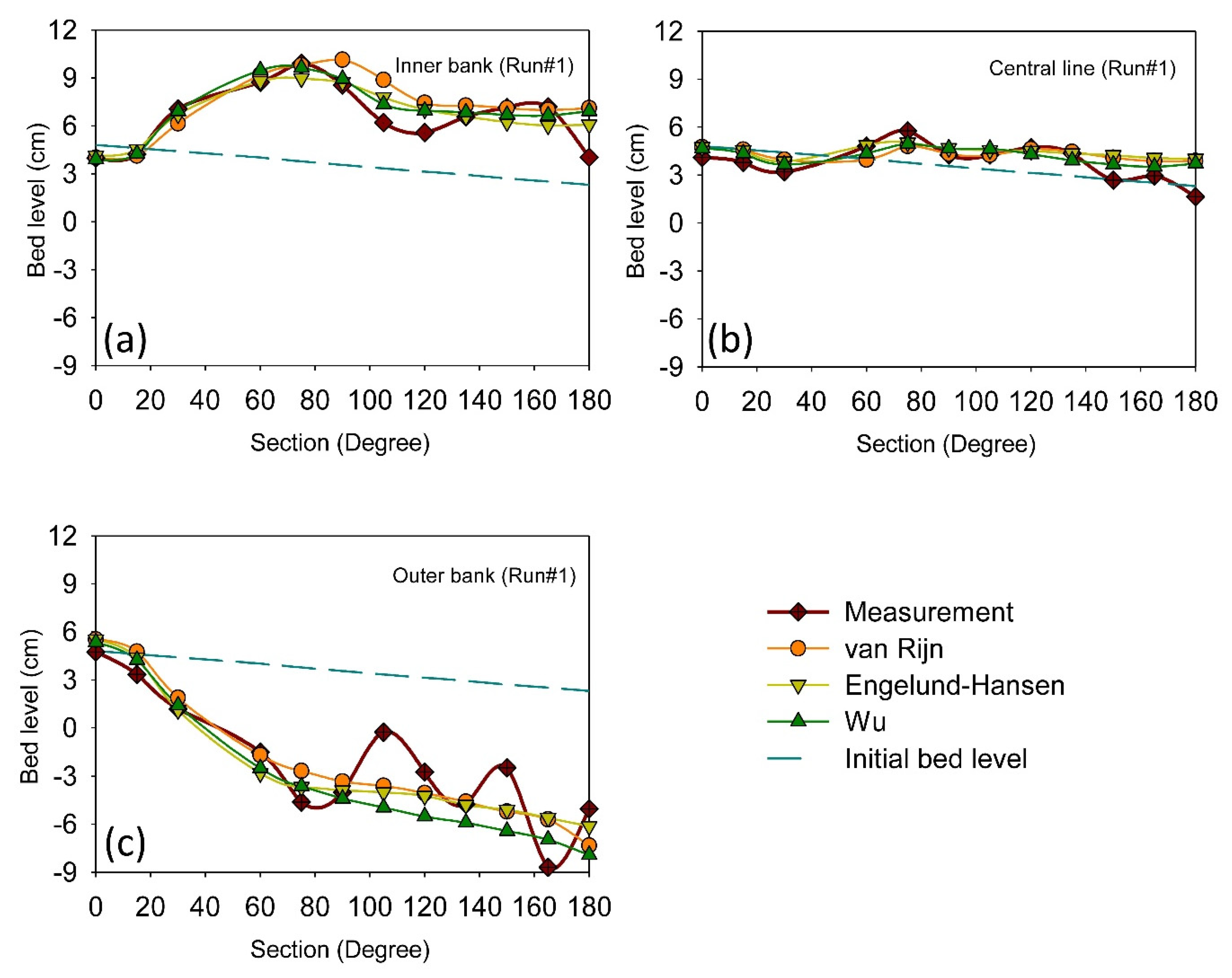
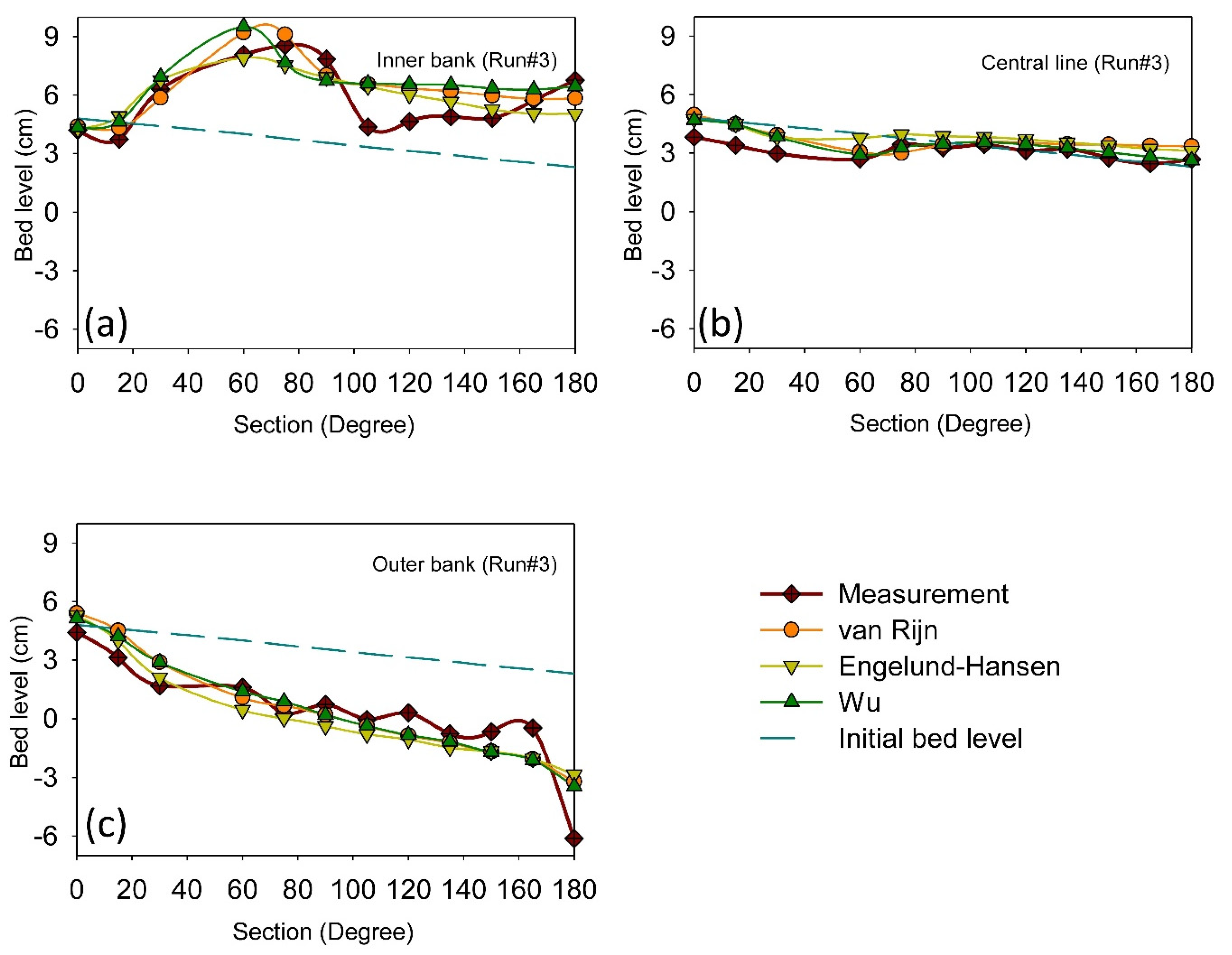
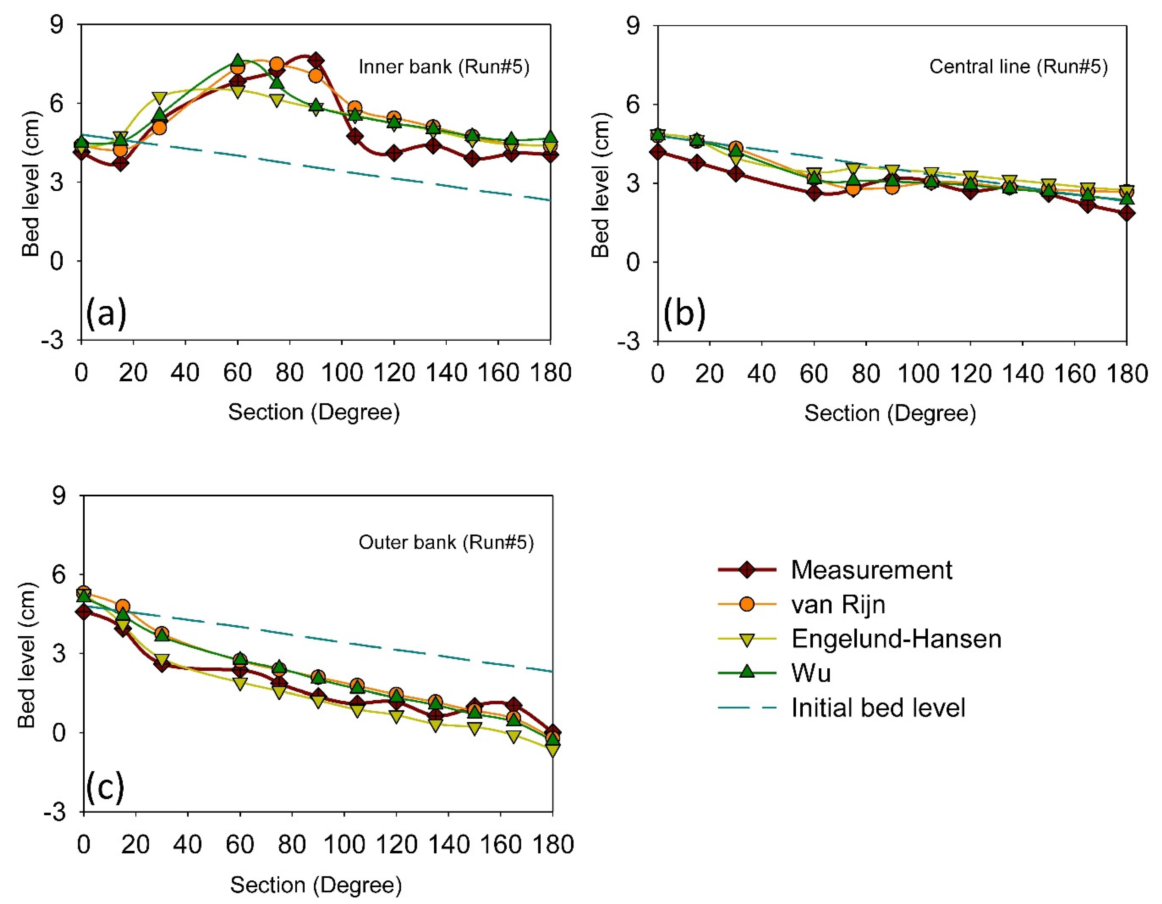
Figure 1, Figure 2 and Figure 3 show longitudinal sections of the initial and final bed levels after Run#1 (the highest discharge), Run#3 (the mid discharge), and Run#5 (the lowest discharge), respectively. The results are presented along the sections: (a) 10 cm from the inner convex bank, (b) the central line, and (c) 10 cm from the outer concave bank.
In Run#1, according to the measurements, the maximum deposition occurs near the inner wall at the 75° cross-section, which is well predicted in terms of position and magnitude by the numerical model using the formula of Wu. The model using Engelund-Hansen’s formula also predicts the location of this point at the same cross-section (75°), with just a minor discrepancy. Nevertheless, the model of van Rijn shows higher bed levels compared to the measurements. In this case, the position of the point bar is at the central cross-section (90°), having a slightly higher magnitude (Figure 1a). Along the central longitudinal-section (Figure 1b), the predicted patterns of bed elevations by all of the numerical models have a similar trend compared to the measurements, with a modest overestimation of the deposition for the last 40° range of the bend (140°–180°). Near the outer bend, the maximum scour depth in the experiment can be seen at the 165° cross-section, whereas the numerical models give this point at the 180° cross-section. In the second half of the bend (90°–180°), measurements show larger fluctuations caused by the development of bedforms compared to the smoother patterns obtained from the simulations (Figure 1c).
Regarding Run#3, near the inner bank, the maximum calculated deposition point is slightly shifted to the upstream compared to the experiment. The location of this point is at around 60°–70° according to the numerical models, although measurements show it at about 75° (Figure 2a). Additionally, in the range of 90°–160°, higher bed levels can be seen in the numerical models compared to the experiment. Along the central line (Figure 2b), numerical models marginally underpredict the erosion part up to the 60° cross-section. However, the overall patterns of the bed levels are similar to the experiment. Although having almost identical patterns near the outer bend (Figure 2c), a contrast can be found in the range of the last 30° of the bend between the simulations and measurements, especially the underestimation of the maximum erosion depth at the 180° cross-section.
In Run#5, similar to Run#3, the position of the maximum bed level near the inner wall (Figure 3a) is shifted further to the upstream in the numerical models. Here, the results of the model using Engelund-Hansen’s formula diverge largely from the measured data. Although showing some degree of underprediction regarding the erosion part up to the 60° cross-section, the simulated bed levels along the central line and near the concave bank are in good agreement with the experimental data (Figure 3b,c).
In Figure 4a–f, the cross-sectional bed profiles for all three runs are plotted at the locations of the maximum deposition height (Run#1: 75°; Run#3: 75°; Run#5: 90°) and the maximum scour depth (Run#1: 165°; Run#3: 180°; Run#5: 180°), according to the experiments. It can be seen that the results of the numerical models are in good agreement with the experimental data regarding the pattern and magnitude of the bed levels. However, the models using the formula of Engelund-Hansen are not successful in accurately predicting the steepness of the scour flank and its depth in the downstream part while increasing the discharge rate (compare Figure 4b,d,f).
According to Table 5, which presents the overall performance of the models based on the coefficient of determination (R2) and the root mean squared error (RMSE) statistics, all three calibrated models using Wu’s formula have the best agreement with the observations, with R2 values ranging between 0.89 and 0.95 and RMSE values ranging between 0.67 cm and 1.49 cm. The simulation results with van Rijn’s formula show similar statistical performance as those obtained with Wu’s formula. Nevertheless, the results for the models using Engelund-Hansen’s formula have the lowest correlation and the highest error compared to the measured data.
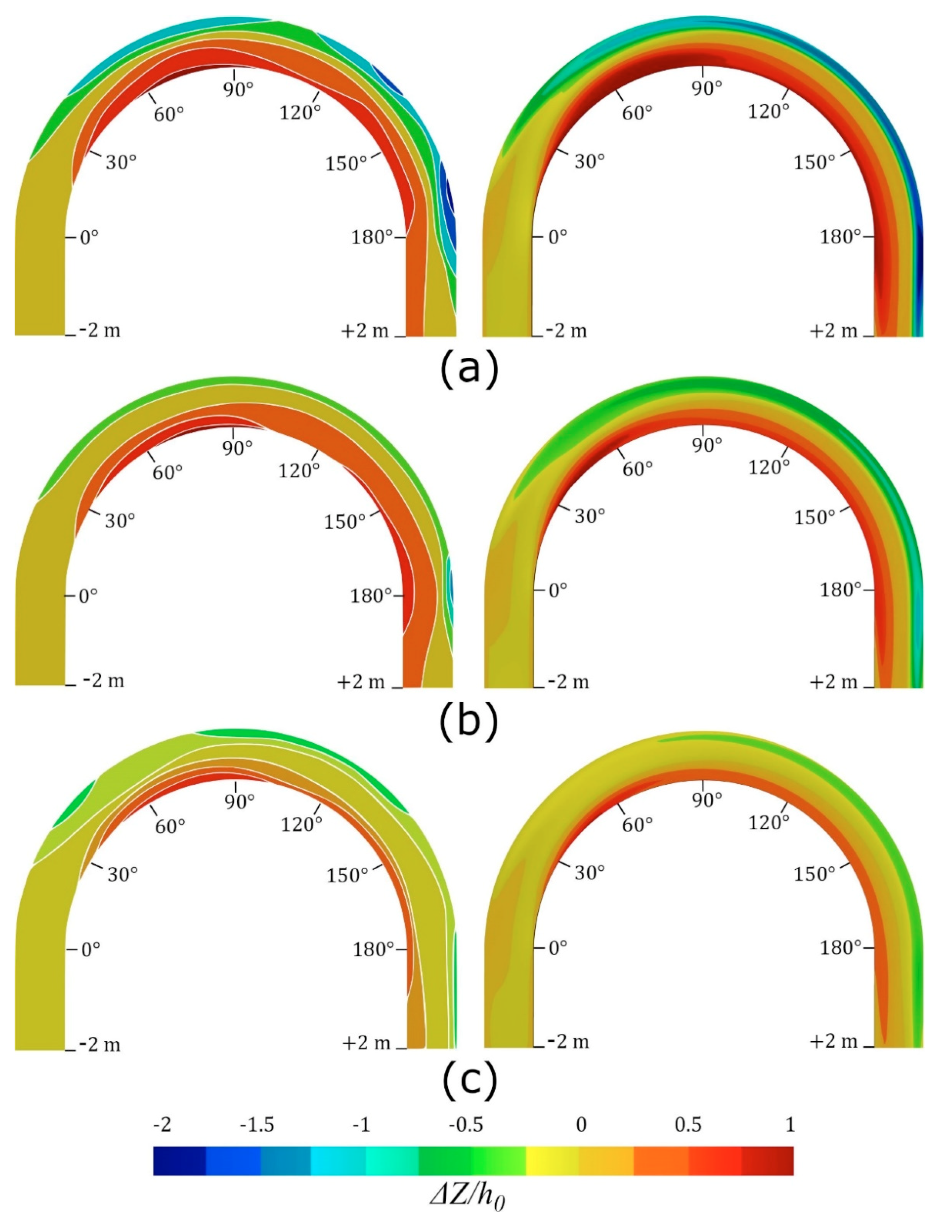
In Figure 5, the bed level changes normalized by the base water depth (ΔZ/h0, where h0 = 5.44 cm) are presented for all runs using Wu’s formula (right side), and are compared with the experimental data (left side).
4. Summary and Conclusions
In the present study, four different optimization methods (GML, SCE-UA, CMA-ES, and PSO) are employed for automatic calibration of a 3D morphodynamic numerical model of a 180° bend. Three input parameters, namely roughness height, active layer thickness, and the sediment volume compared to water at the bed, are selected for calibration, using their initial values and a reasonable range based on the literature. The results of the model calibration using all optimization methods (a local method and three global methods) show very similar calibrated values. All of the methods facilitate the calibration process by reducing the user intervention. However, considering the convergence speed, using the GML algorithm of PEST software is considerably more efficient compared to the other methods, as it needs far fewer model runs. Accordingly, PEST is selected for further investigation (In total, nine models are calibrated by using three different discharge rates and the sediment transport formulae of van Rijn, Wu, and Engelund-Hansen). Nonetheless, as PEST uses a gradient-based algorithm, it potentially involves a high risk of being trapped in a local minimum point over the search space rather than finding the global minimum. Therefore, the initial parameter values should be taken with care. It is also worthwhile reassessing the calibration procedure with different starting values to ensure that PEST finds the global minimum of the objective function. Moreover, characters and discontinuous values, which are defined in models (such as the selection of the sediment transport formula), cannot be processed by PEST and have to be adjusted manually.
The final bed levels predicted by the calibrated numerical models are compared with the measurements at various longitudinal and cross-sections. The overall capabilities of the numerical models are evaluated using the coefficient of determination and the root mean squared error statistics. It is concluded that the calibrated models using Wu’s formula can predict the general characteristics of bed deformations (regions of deposition, erosion, and their magnitudes) better than the other two formulae by having the highest correlation and the lowest error between simulations and experimental data. The formula of van Rijn also gives reasonably acceptable results. However, the models which use the formula of Engelund-Hansen have the highest disagreement with the observations. It can also be mentioned that the bedforms, developed at the outer bend by increasing the discharge rate, cannot be accurately simulated by the numerical model. This effect is independent of the selection of the sediment transport formula and the calibration routine.
Author Contributions
Conceptualization, V.S., S.W., and S.H.; methodology, V.S. and S.H.; software, V.S.; validation, V.S., S.W., and S.H.; formal analysis, V.S. and S.H.; investigation, V.S., S.W., and S.H.; resources, V.S. and S.H.; data curation, V.S. and S.H.; writing—original draft preparation, V.S.; writing—review and editing, V.S., S.W., and S.H.; visualization, V.S.; supervision, S.W.; project administration, S.H. All authors have read and agreed to the published version of the manuscript.
Funding
This research received no external funding.
Acknowledgments
The first author received a Ph.D. scholarship from the German Federal Ministry of Education and Research (BMBF) through the German Academic Exchange Service (DAAD scholarship program NaWaM.
Conflicts of Interest
The authors declare no conflict of interest.
References
- McIntyre, N.; Wheater, H.; Lees, M. Estimation and propagation of parametric uncertainty in environmental models. J. Hydroinf. 2002, 4, 177–198. [Google Scholar] [CrossRef]
- Thomann, R.V. The future “golden age” of predictive models for surface water quality and ecosystem management. J. Environ. Eng. 1998, 124, 94–103. [Google Scholar] [CrossRef]
- Cunge, J.A. Of data and models. J. Hydroinf. 2003, 5, 75–98. [Google Scholar] [CrossRef] [Green Version]
- Oberkampf, W.L.; Trucano, T.G.; Hirsch, C. Verification, validation, and predictive capability in computational engineering and physics. Appl. Mech. Rev. 2004, 57, 345–384. [Google Scholar] [CrossRef] [Green Version]
- Kleijnen, J.P.C. Verification and validation of simulation models. Eur. J. Oper. Res. 1995, 82, 145–162. [Google Scholar] [CrossRef] [Green Version]
- Oreskes, N.; Shrader-Frechette, K.; Belitz, K. Verification, validation, and confirmation of numerical models in the earth sciences. Science 1994, 263, 641–646. [Google Scholar] [CrossRef] [Green Version]
- Bahremand, A.; De Smedt, F. Distributed hydrological modeling and sensitivity analysis in Torysa Watershed, Slovakia. Water Resour. Manag. 2008, 22, 393–408. [Google Scholar] [CrossRef]
- Muleta, M.K.; Nicklow, J.W. Sensitivity and uncertainty analysis coupled with automatic calibration for a distributed watershed model. J. Hydrol. 2005, 306, 127–145. [Google Scholar] [CrossRef] [Green Version]
- Sargent, R.G. Verification and validation of simulation models. J. Simul. 2013, 7, 12–24. [Google Scholar] [CrossRef] [Green Version]
- Oberkampf, W.L.; Trucano, T.G. Verification and validation benchmarks. Nucl. Eng. Des. 2008, 238, 716–743. [Google Scholar] [CrossRef] [Green Version]
- Rebba, R.; Mahadevan, S.; Huang, S. Validation and error estimation of computational models. Reliab. Eng. Syst. Saf. 2006, 91, 1390–1397. [Google Scholar] [CrossRef]
- Refsgaard, J.C.; Henriksen, H.J. Modelling guidelines—Terminology and guiding principles. Adv. Water Resour. 2004, 27, 71–82. [Google Scholar] [CrossRef]
- Acuña, G.J.; Ávila, H.; Canales, F.A. River model calibration based on design of experiments theory. A case study: Meta River, Colombia. Water 2019, 11, 1382. [Google Scholar]
- Troy, T.J.; Wood, E.F.; Sheffield, J. An efficient calibration method for continental-scale land surface modeling: Efficient calibration for large-scale land surface modeling. Water Resour. Res. 2008. [Google Scholar] [CrossRef]
- Hogue, T.S.; Sorooshian, S.; Gupta, H.; Holz, A.; Braatz, D. A multistep automatic calibration scheme for river forecasting models. J. Hydrometeorol. 2000, 1, 524–542. [Google Scholar] [CrossRef]
- Madsen, H. Automatic calibration of a conceptual rainfall–runoff model using multiple objectives. J. Hydrol. 2000, 235, 276–288. [Google Scholar] [CrossRef]
- Moradkhani, H.; Sorooshian, S. General review of rainfall-runoff modeling: Model calibration, data assimilation, and uncertainty analysis. In Hydrological Modelling and the Water Cycle; Sorooshian, S., Hsu, K.-L., Coppola, E., Tomassetti, B., Verdecchia, M., Visconti, G., Eds.; Springer: Berlin/Heidelberg, Germany, 2008; Volume 63, pp. 1–24. [Google Scholar]
- Madsen, H.; Wilson, G.; Ammentorp, H.C. Comparison of different automated strategies for calibration of rainfall-runoff models. J. Hydrol. 2002, 261, 48–59. [Google Scholar] [CrossRef]
- Boyle, D.P.; Gupta, H.V.; Sorooshian, S. Toward improved calibration of hydrologic models: Combining the strengths of manual and automatic methods. Water Resour. Res. 2000, 36, 3663–3674. [Google Scholar] [CrossRef]
- Gupta, H.V.; Sorooshian, S.; Yapo, P.O. Status of automatic calibration for hydrologic models: Comparison with multilevel expert calibration. J. Hydrol. Eng. 1999, 4, 135–143. [Google Scholar] [CrossRef]
- Botterweg, P. The user’s influence on model calibration results: An example of the model SOIL, independently calibrated by two users. Ecol. Model. 1995, 81, 71–81. [Google Scholar] [CrossRef]
- Vidal, J.-P.; Moisan, S.; Faure, J.-B.; Dartus, D. River model calibration, from guidelines to operational support tools. Environ. Model. Softw. 2007, 22, 1628–1640. [Google Scholar] [CrossRef] [Green Version]
- Vidal, J.-P.; Moisan, S.; Faure, J.-B.; Dartus, D. Towards a reasoned 1D river model calibration. J. Hydroinf. 2005, 7, 91–104. [Google Scholar] [CrossRef] [Green Version]
- Madsen, H. Parameter estimation in distributed hydrological catchment modelling using automatic calibration with multiple objectives. Adv. Water Resour. 2003, 26, 205–216. [Google Scholar] [CrossRef]
- Mugunthan, P.; Shoemaker, C.A.; Regis, R.G. Comparison of function approximation, heuristic, and derivative-based methods for automatic calibration of computationally expensive groundwater bioremediation models. Water Resour. Res. 2005. [Google Scholar] [CrossRef] [Green Version]
- Abbaspour, K.C.; Schulin, R.; van Genuchten, M.T. Estimating unsaturated soil hydraulic parameters using ant colony optimization. Adv. Water Resour. 2001, 24, 827–841. [Google Scholar] [CrossRef]
- Finley, J.R.; Pintér, J.D.; Satish, M.G. Automatic model calibration applying global optimization techniques. Environ. Model. Assess. 1998, 3, 117–126. [Google Scholar] [CrossRef]
- Beven, K. A manifesto for the equifinality thesis. J. Hydrol. 2006, 320, 18–36. [Google Scholar] [CrossRef] [Green Version]
- Beven, K. Prophecy, reality and uncertainty in distributed hydrological modelling. Adv. Water Resour. 1993, 16, 41–51. [Google Scholar] [CrossRef]
- Straten, G.T.V.; Keesman, K.J. Uncertainty propagation and speculation in projective forecasts of environmental change: A lake-eutrophication example. J. Forecast. 1991, 10, 163–190. [Google Scholar] [CrossRef]
- Beven, K.; Binley, A. GLUE: 20 years on. Hydrol. Process. 2014, 28, 5897–5918. [Google Scholar] [CrossRef] [Green Version]
- Beven, K.; Freer, J. Equifinality, data assimilation, and uncertainty estimation in mechanistic modelling of complex environmental systems using the GLUE methodology. J. Hydrol. 2001. [Google Scholar] [CrossRef]
- Beven, K.; Binley, A. The future of distributed models: Model calibration and uncertainty prediction. Hydrol. Process. 1992, 6, 279–298. [Google Scholar] [CrossRef]
- Bates, B.C.; Campbell, E.P. A markov Chain Monte Carlo scheme for parameter estimation and inference in conceptual rainfall-runoff modeling. Water Resour. Res. 2001, 37, 937–947. [Google Scholar] [CrossRef]
- Razavi, S.; Tolson, B.A.; Matott, L.S.; Thomson, N.R.; MacLean, A.; Seglenieks, F.R. Reducing the computational cost of automatic calibration through model preemption: Model preemption approach in automatic calibration. Water Resour. Res. 2010. [Google Scholar] [CrossRef]
- Meert, P.; Pereira, F.; Willems, P. Surrogate modeling-based calibration of hydrodynamic river model parameters. J. Hydro. Environ. Res. 2018, 19, 56–67. [Google Scholar] [CrossRef]
- Deslauriers, S.; Mahdi, T.-F. Flood modelling improvement using automatic calibration of two dimensional river software SRH-2D. Nat. Hazards 2018, 91, 697–715. [Google Scholar] [CrossRef]
- Evangelista, S.; Giovinco, G.; Kocaman, S. A multi-parameter calibration method for the numerical simulation of morphodynamic problems. J. Hydrol. Hydromech. 2017, 65, 175–182. [Google Scholar] [CrossRef] [Green Version]
- Lavoie, B.; Mahdi, T.-F. Comparison of two-dimensional flood propagation models: SRH-2D and Hydro_AS-2D. Nat. Hazards 2017, 86, 1207–1222. [Google Scholar] [CrossRef] [Green Version]
- McKibbon, J.; Mahdi, T.-F. Automatic calibration tool for river models based on the MHYSER software. Nat. Hazards 2010, 54, 879–899. [Google Scholar] [CrossRef]
- Fabio, P.; Aronica, G.T.; Apel, H. Towards automatic calibration of 2-D flood propagation models. Hydrol. Earth Syst. Sci. 2010, 14, 911–924. [Google Scholar] [CrossRef] [Green Version]
- Wasantha Lal, A.M. Calibration of riverbed roughness. J. Hydraul. Eng. 1995, 121, 664–671. [Google Scholar] [CrossRef]
- Doherty, J. PEST Model-Independent Parameter Estimation User Manual Part I, 6th ed.; Watermark Numerical Computing: Brisbane, Australia, 2016. [Google Scholar]
- Kennedy, J.; Eberhart, R. Particle swarm optimization. In Proceedings of the ICNN’95—International Conference on Neural Networks, Perth, WA, Australia, 27 November–1 December 1995; Volume 4, pp. 1942–1948. [Google Scholar]
- Duan, Q.; Sorooshian, S.; Gupta, V. Effective and efficient global optimization for conceptual rainfall-runoff models. Water Resour. Res. 1992, 28, 1015–1031. [Google Scholar] [CrossRef]
- Hansen, N.; Ostermeier, A. Adapting arbitrary normal mutation distributions in evolution strategies: The covariance matrix adaptation. In Proceedings of the IEEE International Conference on Evolutionary Computation, Nagoya, Japan, 20–22 May 1996. [Google Scholar]
- Yen, C.; Lee, K.T. Bed topography and sediment sorting in channel bend with unsteady flow. J. Hydraul. Eng. 1995, 121, 591–599. [Google Scholar] [CrossRef]
- Ferguson, R.I.; Church, M. A Simple universal equation for grain settling velocity. J. Sediment. Res. 2004, 74, 933–937. [Google Scholar] [CrossRef]
- Olsen, N.R.B. A Three Dimensional Numerical Model for Simulation of Sediment Movement in Water Intakes with Multiblock Option; Department of Hydraulic and Environmental Engineering, The Norwegian University of Science and Technology: Trondheim, Norway, 2014. [Google Scholar]
- Saam, L.; Mouris, K.; Wieprecht, S.; Haun, S. Three-dimensional numerical modelling of reservoir flushing to obtain long-term sediment equilibrium. In Proceedings of the 38th IAHR World Congress, Panama City, Panama, 1–6 September 2019. [Google Scholar]
- Mouris, K.; Beckers, F.; Haun, S. Three-dimensional numerical modeling of hydraulics and morphodynamics of the Schwarzenbach reservoir. E3s Web Conf. 2018, 40, 03005. [Google Scholar] [CrossRef]
- Esmaeili, T.; Sumi, T.; Kantoush, S.; Kubota, Y.; Haun, S.; Rüther, N. Three-dimensional numerical study of free-flow sediment flushing to increase the flushing efficiency: A case-study reservoir in Japan. Water 2017, 9, 900. [Google Scholar] [CrossRef] [Green Version]
- Harb, G.; Haun, S.; Schneider, J.; Olsen, N.R.B. Numerical analysis of synthetic granulate deposition in a physical model study. Int. J. Sediment Res. 2014, 29, 110–117. [Google Scholar] [CrossRef]
- Haun, S.; Kjærås, H.; Løvfall, S.; Olsen, N.R.B. Three-dimensional measurements and numerical modelling of suspended sediments in a hydropower reservoir. J. Hydrol. 2013, 479, 180–188. [Google Scholar] [CrossRef]
- Haun, S.; Olsen, N.R.B. Three-dimensional numerical modelling of the flushing process of the Kali Gandaki hydropower reservoir. Lakes Reserv. Sci. Policy Manag. Sustain. Use 2012, 17, 25–33. [Google Scholar] [CrossRef]
- Haun, S.; Olsen, N.R.B.; Feurich, R. Numerical modeling of flow over trapezoidal broad-crested weir. Eng. Appl. Comput. Fluid Mech. 2011, 5, 397–405. [Google Scholar] [CrossRef] [Green Version]
- Wilson, C.A.M.E.; Yagci, O.; Rauch, H.-P.; Olsen, N.R.B. 3D numerical modelling of a willow vegetated river/floodplain system. J. Hydrol. 2006, 327, 13–21. [Google Scholar] [CrossRef]
- Rüther, N.; Olsen, N.R. Three-dimensional modeling of sediment transport in a narrow 90° channel bend. J. Hydraul. Eng. 2005, 131, 917–920. [Google Scholar] [CrossRef]
- Olsen, N.R.B. Three-dimensional CFD modeling of self-forming meandering channel. J. Hydraul. Eng. 2003, 129, 366–372. [Google Scholar] [CrossRef]
- Booker, D.J. Hydraulic modelling of fish habitat in urban rivers during high flows. Hydrol. Process. 2003, 17, 577–599. [Google Scholar] [CrossRef]
- Wilson, C.A.M.E.; Boxall, J.B.; Guymer, I.; Olsen, N.R.B. Validation of a three-dimensional numerical code in the simulation of pseudo-natural meandering flows. J. Hydraul. Eng. 2003, 129, 758–768. [Google Scholar] [CrossRef]
- Versteeg, H.K.; Malalasekera, W. An Introduction to Computational Fluid Dynamics: The Finite Volume Method, 2nd ed.; Pearson Education Ltd.: Harlow, UK, 2007. [Google Scholar]
- Patankar, S.V. Numerical Heat Transfer and Fluid Flow; McGraw-Hill: New York, NY, USA, 1980. [Google Scholar]
- Rodi, W. Turbulence Models and Their Application in Hydraulics, 1st ed.; Routledge: Rotterdam, The Netherlands, 1993. [Google Scholar]
- Olsen, N.R.B.; Haun, S. Free surface algorithms for 3D numerical modelling of reservoir flushing. In Proceedings of the River flow 2010, Federal Waterways Engineering and Research Institute (BAW), Braunschweig, Germany, 8–10 September 2010; Volume 2010, pp. 1105–1110. [Google Scholar]
- Schlichting, H. Boundary Layer Theory; McGraw-Hill: New York, NY, USA, 1979. [Google Scholar]
- Fischer-Antze, T.; Rüther, N.; Olsen, N.R.B.; Gutknecht, D. Three-dimensional (3D) modeling of non-uniform sediment transport in a channel bend with unsteady flow. J. Hydraul. Res. 2009, 47, 670–675. [Google Scholar] [CrossRef]
- Haun, S.; Olsen, N.R.B. Three-dimensional numerical modelling of reservoir flushing in a prototype scale. Int. J. River Basin Manag. 2012, 10, 341–349. [Google Scholar] [CrossRef]
- Engelund, F.; Hansen, E. A Monograph on Sediment Transport in Alluvial Streams; Teknisk Vorlag: Copenhagen, Denmark, 1967. [Google Scholar]
- Van Rijn, L.C. Sediment transport, part I: Bed load transport. J. Hydraul. Eng. 1984, 110, 1431–1456. [Google Scholar] [CrossRef] [Green Version]
- Wu, W.; Wang, S.S.Y.; Jia, Y. Nonuniform sediment transport in alluvial rivers. J. Hydraul. Res. 2000, 38, 427–434. [Google Scholar] [CrossRef]
- Soltani, M.; Laux, P.; Mauder, M.; Kunstmann, H. Inverse distributed modelling of streamflow and turbulent fluxes: A sensitivity and uncertainty analysis coupled with automatic optimization. J. Hydrol. 2019, 571, 856–872. [Google Scholar] [CrossRef]
- Usman, M.; Reimann, T.; Liedl, R.; Abbas, A.; Conrad, C.; Saleem, S. Inverse parametrization of a regional groundwater flow model with the aid of modelling and GIS: Test and application of different approaches. ISPRS Int. J. Geo. Inf. 2018, 7, 22. [Google Scholar] [CrossRef] [Green Version]
- Necpálová, M.; Anex, R.P.; Fienen, M.N.; Del Grosso, S.J.; Castellano, M.J.; Sawyer, J.E.; Iqbal, J.; Pantoja, J.L.; Barker, D.W. Understanding the DayCent model: Calibration, sensitivity, and identifiability through inverse modeling. Environ. Model. Softw. 2015, 66, 110–130. [Google Scholar] [CrossRef] [Green Version]
- Rode, M.; Suhr, U.; Wriedt, G. Multi-objective calibration of a river water quality model—Information content of calibration data. Ecol. Model. 2007, 204, 129–142. [Google Scholar] [CrossRef]
- Baginska, B.; Milne-Home, W.; Cornish, P.S. Modelling nutrient transport in Currency Creek, NSW with AnnAGNPS and PEST. Environ. Model. Softw. 2003, 18, 801–808. [Google Scholar] [CrossRef]
- Liu, C.; Batelaan, O.; Smedt, F.D.; Poórová, J.; Velcická, L. Automated calibration applied to a GIS-based flood simulation model using PEST. In Floods, from Defence to Management; van Alphen, J., van Beek, E., Taal, M., Eds.; Taylor-Francis Group: London, UK, 2005; pp. 317–326. [Google Scholar]
- Marquardt, D.W. An algorithm for least-squares estimation of nonlinear parameters. J. Soc. Ind. Appl. Math. 1963, 11, 431–441. [Google Scholar] [CrossRef]
- Levenberg, K. A method for the solution of certain nonlinear problems in least squares. Q. Appl. Math. 1944, 2, 164–168. [Google Scholar] [CrossRef] [Green Version]
- Holland, J.H. Adaptation in Natural and Artificial Systems: An Introductory Analysis with Applications to Biology, Control and Artificial Intelligence; MIT Press: Cambridge, MA, USA, 1992. [Google Scholar]
- Nelder, J.A.; Mead, R. A simplex method for function minimization. Comput. J. 1965, 7, 308–313. [Google Scholar] [CrossRef]
- Price, W.L. Global optimization algorithms for a CAD workstation. J. Optim. Theory Appl. 1987, 55, 133–146. [Google Scholar] [CrossRef]
- Duan, Q.; Sorooshian, S.; Gupta, V.K. Optimal use of the SCE-UA global optimization method for calibrating watershed models. J. Hydrol. 1994, 158, 265–284. [Google Scholar] [CrossRef]
- Duan, Q.Y.; Gupta, V.K.; Sorooshian, S. Shuffled complex evolution approach for effective and efficient global minimization. J. Optim. Theory Appl. 1993, 76, 501–521. [Google Scholar] [CrossRef]
- Hansen, N. The CMA evolution strategy: A tutorial. arXiv 2016, arXiv:1604.00772. [Google Scholar]
- Shi, Y.; Eberhart, R.C. Parameter selection in particle swarm optimization. In Evolutionary Programming VII; Porto, V.W., Saravanan, N., Waagen, D., Eiben, A.E., Eds.; Springer: Berlin/Heidelberg, Germany, 1998; pp. 591–600. [Google Scholar]
- García, M.H. Sedimentation Engineering: Processes, Measurements, Modeling, and Practice; Environmental and Water Resources Institute (EWRI), ASCE Manuals and Reports on Engineering Practice, American Society of Civil Engineers: Reston, VA, USA, 2008. [Google Scholar]
- Hunziker, R.P. Fraktionsweiser Geschiebetransport. Ph.D. Thesis, ETH, Zurich, Switzerland, 1995. [Google Scholar]
- Malcherek, A. Sedimenttransport und Morphodynamik; Scriptum Institut für Wasserwesen, Bundeswehr University Munich: Munich, Germany, 2007. [Google Scholar]
Figure 1.
Initial and final bed levels of Run#1 along three longitudinal sections, (a) 10 cm from the inner bank, (b) the central line, and (c) 10 cm from the outer bank.
Figure 1.
Initial and final bed levels of Run#1 along three longitudinal sections, (a) 10 cm from the inner bank, (b) the central line, and (c) 10 cm from the outer bank.

Figure 2.
Initial and final bed levels of Run#3 along three longitudinal sections, (a) 10 cm from the inner bank, (b) the central line, and (c) 10 cm from the outer bank.
Figure 2.
Initial and final bed levels of Run#3 along three longitudinal sections, (a) 10 cm from the inner bank, (b) the central line, and (c) 10 cm from the outer bank.

Figure 3.
Initial and final bed levels of Run#5 along three longitudinal sections, (a) 10 cm from the inner bank, (b) the central line, and (c) 10 cm from the outer bank.
Figure 3.
Initial and final bed levels of Run#5 along three longitudinal sections, (a) 10 cm from the inner bank, (b) the central line, and (c) 10 cm from the outer bank.

Figure 4.
Cross-sectional bed levels for all runs in the maximum deposition (a,c,e) and erosion (b,d,f) sections according to the experiments.
Figure 4.
Cross-sectional bed levels for all runs in the maximum deposition (a,c,e) and erosion (b,d,f) sections according to the experiments.

Figure 5.
Plan view of the normalized bed deformations for (a) Run#1, (b) Run#3, and (c) Run#5, comparing the simulations (right) to the measurements (left).
Figure 5.
Plan view of the normalized bed deformations for (a) Run#1, (b) Run#3, and (c) Run#5, comparing the simulations (right) to the measurements (left).


Table 1.
Sediment characteristics of the experiments that were applied in the numerical model.
| Sediment Size Classes | ||||||||
|---|---|---|---|---|---|---|---|---|
| Size (mm) | 0.25 | 0.42 | 0.84 | 1.19 | 2.00 | 3.36 | 4.76 | 8.52 |
| Proportion (%) | 6.55 | 10.56 | 25.36 | 15.06 | 20.11 | 13.02 | 4.88 | 4.46 |
| Cumulative proportion (%) | 6.55 | 17.11 | 42.47 | 57.53 | 77.64 | 90.66 | 95.54 | 100 |
| Fall velocity (m/s) | 0.03 | 0.06 | 0.11 | 0.14 | 0.20 | 0.26 | 0.32 | 0.43 |
Table 2.
Characteristics of the three hydrographs used in this study.
| Run# | Peak Flow Discharge (m3/s) | Peak Flow Depth (cm) | Duration (min) |
|---|---|---|---|
| 1 | 0.0750 | 12.9 | 180 |
| 3 | 0.0613 | 11.3 | 240 |
| 5 | 0.0436 | 9.10 | 420 |
Table 3.
Calibration results for the numerical model Run#5 by local and global optimization methods, using Wu’s sediment transport formula.
Table 3.
Calibration results for the numerical model Run#5 by local and global optimization methods, using Wu’s sediment transport formula.
| Calibration Results | Calibration Method | ||||||
|---|---|---|---|---|---|---|---|
| PEST#1 | PEST#2 | PEST#3 | PEST#4 | SCE-UA | CMA-ES | PSO | |
| ks (cm) | 0.904 | 0.894 | 0.899 | 0.903 | 0.898 | 0.892 | 0.904 |
| ALT (cm) | 1.639 | 1.644 | 1.629 | 1.638 | 1.635 | 1.631 | 1.647 |
| VFS (%) | 48.1 | 47.9 | 48.4 | 48 | 48.1 | 48.1 | 47.9 |
| Minimum of SSR (cm) | 0.28249 | 0.28251 | 0.28240 | 0.28249 | 0.28247 | 0.28247 | 0.28241 |
| Number of model runs | 26 | 30 | 28 | 27 | 176 | 440 | 448 |
Note: ks, roughness height at the bed; ALT, active layer thickness; VFS, the volume fraction of compacted sediments; SSR, sum of the squared residuals.
Table 4.
Calibrated values of the three selected parameters for nine simulations.
| Calibration Parameters | Sediment Transport Formula | ||||||||
|---|---|---|---|---|---|---|---|---|---|
| Wu | Van Rijn | Engelund-Hansen | |||||||
| Run#1 | Run#3 | Run#5 | Run#1 | Run#3 | Run#5 | Run#1 | Run#3 | Run#5 | |
| ks (cm) | 1.52 | 1.34 | 0.90 | 0.63 | 0.61 | 0.37 | 0.48 | 0.31 | 0.25 |
| ALT (cm) | 2.04 | 1.85 | 1.64 | 2.20 | 1.94 | 1.24 | 1.31 | 1.12 | 0.74 |
| VFS (%) | 49 | 51 | 48 | 60 | 60 | 60 | 52 | 51 | 53 |
Table 5.
Goodness of fit for the calibrated models with different sediment transport formulae.
| Goodness of Fit | Sediment Transport Formula | ||||||||
|---|---|---|---|---|---|---|---|---|---|
| Wu | Van Rijn | Engelund-Hansen | |||||||
| Run#1 | Run#3 | Run#5 | Run#1 | Run#3 | Run#5 | Run#1 | Run#3 | Run#5 | |
| R2 (-) | 0.90 | 0.89 | 0.95 | 0.90 | 0.89 | 0.94 | 0.88 | 0.83 | 0.90 |
| RMSE (cm) | 1.49 | 1.04 | 0.67 | 1.57 | 1.08 | 0.69 | 1.63 | 1.33 | 0.81 |
Note: R2, the coefficient of determination; RMSE, the root mean squared error.
© 2020 by the authors. Licensee MDPI, Basel, Switzerland. This article is an open access article distributed under the terms and conditions of the Creative Commons Attribution (CC BY) license (http://creativecommons.org/licenses/by/4.0/).
Share and Cite
MDPI and ACS Style
Shoarinezhad, V.; Wieprecht, S.; Haun, S. Comparison of Local and Global Optimization Methods for Calibration of a 3D Morphodynamic Model of a Curved Channel. Water 2020, 12, 1333. https://doi.org/10.3390/w12051333
AMA Style
Shoarinezhad V, Wieprecht S, Haun S. Comparison of Local and Global Optimization Methods for Calibration of a 3D Morphodynamic Model of a Curved Channel. Water. 2020; 12(5):1333. https://doi.org/10.3390/w12051333
Chicago/Turabian StyleShoarinezhad, Vahid, Silke Wieprecht, and Stefan Haun. 2020. "Comparison of Local and Global Optimization Methods for Calibration of a 3D Morphodynamic Model of a Curved Channel" Water 12, no. 5: 1333. https://doi.org/10.3390/w12051333
Note that from the first issue of 2016, this journal uses article numbers instead of page numbers. See further details here.