Zonation of Positively Buoyant Jets Interacting with the Water-Free Surface Quantified by Physical and Numerical Modelling


IHCantabria—Instituto de Hidráulica Ambiental de la Universidad de Cantabria, Isabel Torres, 15, Parque Científico y Tecnológico de Cantabria, 39011 Santander, Spain
*
Author to whom correspondence should be addressed.
Water 2020, 12(5), 1324; https://doi.org/10.3390/w12051324
Submission received: 3 March 2020
/
Revised: 1 May 2020
/
Accepted: 4 May 2020
/
Published: 7 May 2020
(This article belongs to the Special Issue Physical Modelling in Hydraulics Engineering)
Abstract
:The evolution of positively buoyant jets was studied with non-intrusive techniques—Particle Image Velocimetry (PIV) and Laser Induce Fluorescence (LIF)—by analyzing four physical tests in their four characteristic zones: momentum dominant zone (jet-like), momentum to buoyancy transition zone (jet to plume), buoyancy dominant zone (plume-like), and lateral dispersion dominant zone. Four configurations were tested modifying the momentum and the buoyancy of the effluent through variations of flow discharge and the thermal gradient with the receiving water body, respectively. The physical model results were used to evaluate the performance of numerical models to describe such flows. Furthermore, a new method to delimitate the four characteristic zones of positively buoyant jets interacting with the water-free surface was proposed using the angle (α) shaped by the tangent of the centerline trajectory and the longitudinal axis. Physical model results showed that the dispersion of mass (concentrations) was always greater than the dispersion of energy (velocity) during the evolution of positively buoyant jets. The semiempirical models (CORJET and VISJET) underestimated the trajectory and overestimated the dilution of positively buoyant jets close to the impact zone with the water-free surface. The computational fluid dynamics (CFD) model (Open Field Operation And Manipulation model (OpenFOAM)) is able to reproduce the behavior of positively buoyant jets for all the proposed zones according to the physical results.
1. Introduction
The economic growth throughout the 20th century fostered the establishment of industries near estuarine and coastal zones. Their activities demanded suitable areas for the disposal of their discharges, being buoyant jets. The presence of these discharges together with the high environmental requirements of these water bodies supposes a management challenge [1,2]. These wastewaters can contain physical, chemical and/or biological pollutants and cannot be adequately quantified without actual measuring and testing. Buoyant jets evolution is dominated by momentum and buoyancy. Buoyancy is a density-dependent property. Accordingly, a jet with a lower density than the receiving medium will have a positive buoyancy and will tend to rise to the surface due to gravity forces, known as positively buoyant jets or forced plumes. In the case of negative buoyancy, the discharge will have a higher density than the receiving environment so the jet will tend to descend to the bottom, known as negatively buoyant jets.
Industrial and urban wastewaters are typically freshwaters. They are characterized by a positive buoyancy and an initial momentum when discharging into brackish or salt waters such as estuarine or coastal areas [3]. Among the wastewater disposal techniques, submarine outfalls are widespread around the globe and recommended by several international organizations [4]. These outfalls are typically a single-port discharge located at the bottom of the receiving water body. Their discharge is usually parallel to the main direction of ambient currents [5]. Thus, a fluid with some momentum and/or buoyancy exits from a relatively narrow orifice and intrudes into a larger body of fluid with different characteristics. These flows can be characterized as partly turbulent because they create situations where the turbulence level is much higher near the intrusion than in the surrounding fluid [6].
Physical models with intrusive techniques studied the evolution of positively buoyant jets [7,8,9,10]. According to the buoyancy forces and momentum, these studies achieved the parametrization of a few points of the jet-rising until the impact with the water-free surface. All these works generated semiempirical models which are currently used for the study of positively buoyant jets in the civil engineering field such as CORMIX [11] or VISJET [12]. However, since the effluent is calculated by empirical equations instead of the fluid mechanics equations with specific boundary conditions, only rectangular-like zones with a flat bottom and without interaction with physical boundaries are suitable for the calculations. Consequently, results lose significance when the positively buoyant jet hits the water-free surface. Few labs and field studies examined these interactions in more detail [13]. Although these works generally confirmed negligible effects for positively buoyant jets into reasonable strong turbulent current fields, they clearly showed their importance in either stagnant or shallow waters such as it could be the case of confined areas like reservoirs, dead-zones in estuarine waters or docks areas in harbors [14,15].
To overcome this lack of information, the evolution of positively buoyant jets was analyzed by: (1) non-intrusive techniques such as Particle Image Velocimetry (PIV) [16,17,18,19,20], (2) Laser Induce Fluorescence (LIF) [21,22,23,24,25], and/or (3) simultaneously PIV and LIF [26,27,28,29]. These two techniques provided high-quality results of velocity vector fields and concentration scalar fields at one or several planes of the fluid medium for any discharged substance, respectively.
The uncertainty of semiempirical model results when positively buoyant jets interact with the physical boundaries formed the starting point for computational fluid mechanics (CFD) approaches. CFD models might be helpful for the analysis of special cases, where either experiments are too difficult or too expensive and semiempirical models do not apply [30,31,32], such as the Open Field Operation And Manipulation model (OpenFOAM).
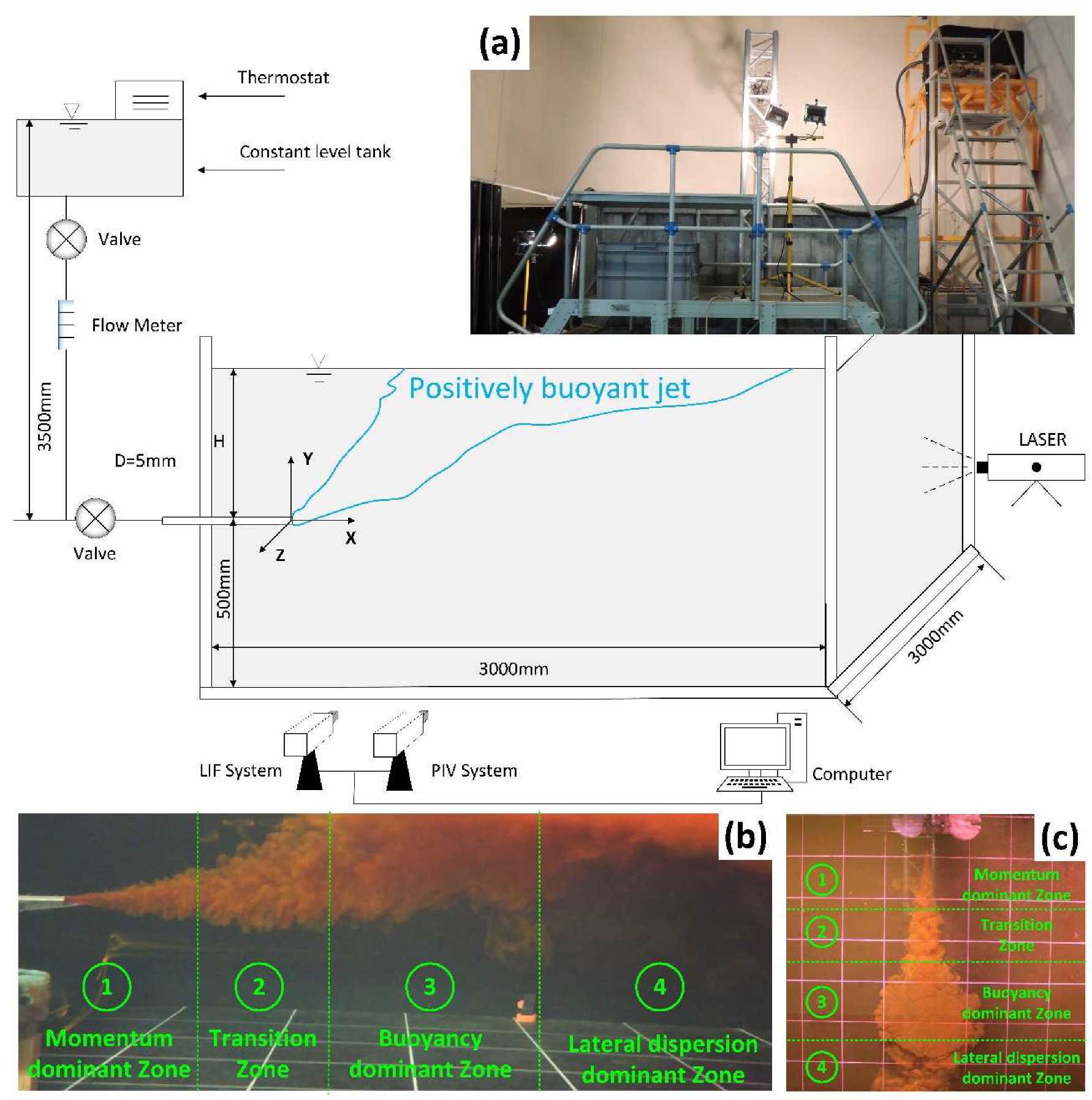
The evolution of positively buoyant jets is generally separated into four zones (see Figure 1b,c), called (Zone 1) momentum dominant zone (jet-like), (Zone 2) momentum to buoyancy transition zone (jet to plume), (Zone 3) buoyancy dominant zone (plume-like), and (Zone 4) lateral dispersion zone, in which different physical and chemical mechanisms govern their trajectory and dilution [11].
In the Zones 1 to 3, the initial jet characteristics of momentum flux, buoyancy flux, and outfall configuration (orientations and geometries) influence the effluent trajectory and dilution. Source induced turbulence entrains ambient fluid and dilutes the effluent [33]. Although ambient characteristics affect the discharge once the effluent left the outfall, they are still only of minor importance [9].
The beginning of the Zone 4 is characterized by the transition from the vertically rising movement to a horizontal motion generated by the gravitational collapse of the effluent cloud [10]. Outfall characteristics become less important. Vertical and horizontal boundary conditions will control trajectory and dilution through buoyant spreading motions and passive diffusion due to interfacial mixing [34]. Finally, ambient conditions control the evolution of positively buoyant jets in the Zone 4 through passive diffusion due to ambient turbulence and passive advection by the often time-varying and non-uniform ambient velocity field [9].
Usually, the buoyant jets have been delimited by length scales based on physical modelling [11,35,36,37]. However, this zonation presents uncertainties because their obtainment is based on semiempirical adjustments with laboratory data that may have associated errors in both measurement and adjustment. The adjustment of these semiempirical formulations used linear fitting on a point cloud, with notable differences between different tests to calculate the length scales for a given buoyant jet. Furthermore, precise information of vertical discretization is needed to analyze the evolution of a jet when its behavior is like a plume evolution and these data are not always available. For instance, this discretization introduces important errors of up to 30% in the jet centerline trajectory and up of 50% in jet centerline dilution [38].
Therefore, this study aims to assess the zonation of positively buoyant jets from its discharge into the receiving water body until its advance in the far-field by proposing a new methodology based on the angle (α) shaped by the tangent of the centerline trajectory and the longitudinal axis. α is a value from which it is possible to define which type of force is dominant over the jet during its advance in a fluid environment. To accomplish this work, the specific objectives are: (1) collecting physical data on the evolution (trajectory and dilution) of positively buoyant jets in a stagnant medium by physical modelling using a coupled PIV-LIF technique, (2) calibrating two semiempirical models (CORJET and VISJET) and one CFD model (OpenFOAM) with the collected data, and (3) applying the proposed method to assess the accuracy of numerical modelling to calculate the zone limits of positively buoyant jets.
2. Materials and Methods
2.1. Physycal Modelling
2.1.1. Description of the PIV and LIF Techniques
PIV is a laser optical technique used for the measurement of instantaneous velocity flow fields. The flow is seeded with suitable tracer particles which are assumed to follow the flow faithfully. These particles scatter light when illuminated by means of a laser. A Charge Coupled Device (CCD) camera, synchronized to the laser, captures several images of the light scattered by each particle within a short time interval. The unit displacement of the particles can then be computed from successive images by means of cross-correlation. Finally, the local velocity is obtained by dividing the displacement over the time interval between the laser pulses [29].
LIF is a technique used in visualization experiments. However, if the experiments are performed carefully, it is possible to attain quantitative concentration measurements. This technique is based on the physical property of certain organic molecules, that allows an electron in the outer orbit to be exited. It moves from one of the vibrational levels of the ground state into the so-called singlet state. A laser is used to excite a fluorescent species within the flow. Typically, the tracer is an organic fluorescent dye such as fluorescein or rhodamine. The dye absorbs a portion of the excitation energy and spontaneously reemits a portion of the absorbed energy as fluorescence. The fluorescence is measured optically and used to infer the local concentration of the dye [39]. Accordingly, LIF system requires an appropriately paired CCD camera, laser and fluorescent dye combination, with the laser frequency within the absorption band of the dye.
The use of PIV and LIF techniques have an advantage over the classical methods when carrying out measurements of velocities and concentrations in a fluid environment because this measurement techniques have an optical nature and they are not intrusive on the flow. Thus, the magnitudes are not disturbed. On the contrary, classic measurements introduce an instrument that obviously influences the flow patterns, such as hot wire anemometry.
2.1.2. Setup of the Physical Modelling
The physical tests were performed at IHCantabria by means of simultaneous PIV and LIF techniques [40,41]. The physical setup comprised (see in Figure 1a): (1) a steel test tank with 3 m length, 3 m width, and 1 m depth, acting as the receiving water body, (2) a 100 L steel constant level tank containing the effluent, (3) a 1000 L plastic effluent storage tank, and (4) a piping system connecting the three tanks.
The test tank was made with two side glass windows. One window was used for illuminating the flow with a laser sheet and, the other window, for imaging the flow. Moreover, walls, bottom and the aluminum discharge tube were painted in black to avoid reflections of the laser during the tests. The nozzle of the discharge tube had a 5 mm inner diameter (D) and was located 50 cm above and parallel to the bottom of the test tank. The discharged flow was measured by an ultrasonic flow meter. The constant level tank contained a computer-controlled thermostat as a heating device (DIGITERM 2000, Selecta) and was located on top of a 5 m structure to obtain a gravity-driven flow as shown in Figure 1a. Furthermore, a recirculating pump was placed inside of the constant level tank to ease the fluid homogenization and to avoid the formation of thermoclines. Finally, the piping system and the walls of the constant level tank were insulated with neoprene to reduce heat losses.
Regarding the PIV and LIF techniques, a Q-switched double pulse Nd-Yag laser was used to illuminate the flow, using a Quantel model Twins BSL140 dual-cavity laser to create a bidimensional sheet, with a thickness between 0.5 and 2.5 mm. The energy level was 130 mJ per pulse and the pulse duration about 8 ns. Light emitted was green with a 532 nm wavelength and with a 30 Hz pulse repetition rate of each cavity. The laser was equipped with a telescopic arm for vertically placing the laser sheet and passing through the center of the discharge tube.
To characterize the trajectory and dilution of the buoyant jet, three cameras were available to record images: two cameras from a stereoscopic PIV system and another camera from a LIF system (LaVision Imager 90 ProX 4M). The stereoscopic PIV system was used as a conventional PIV system, since the system was only focused on the central axis of the jet and the variation in the perpendicular axis to the jet’s advance was not swept away. The cameras were synchronized to take simultaneous measures of velocity and concentration.
The CCD array is a 2048 × 2048 pixel sensor consisting of square detectors 7.4 × 7.4 µm2 with physical dimensions of 15.15 × 15.15 mm2. Each CCD camera was mounted with a Nikon AF Nikkor 50 mm 1:1.8D objective with an aperture varying between 1.8 and 22. The CCD cameras were placed parallel to each other and approximately perpendicular to the laser sheet and the jet centerline. Both cameras had the same horizontal and vertical field-of-view (FOV) of 71 cm with a total overlap of both FOV. One camera took the image at time t and the other camera at t + ∆t. The velocity composition was carried out by an inter-correlation algorithm [42], which divides the two successive images of the recorded particles at time t and t + ∆t into small interrogation areas. The position of the correlation peak between the two images corresponds to the most probable displacement of the particles for each of these interrogation areas [42]. The effects of geometric distortion, resulting from small angles in camera alignment, were automatically corrected during image processing and post-processing using LaVision DaVis software. The cameras were moved forward or backward depending on the test configurations in order to zoom in or zoom out on the flow area. Firstly, the cameras were relocated to define their results in the plane that marks the central axis of the jet advance. Secondly, the cameras were placed in such a way that the plane was wide enough to contain from the start of the jet until it was in the so-called lateral dispersion dominant zone, taking into account the number of pixels available for the camera to define accurately the jet evolution.
The LIF camera has a band-pass filter, which allows only the fluorescent light emitted from the tracer dye excited by the laser to pass through. The filter ensures an excellent blocking efficiency of the excitation wavelength with a steep edge at 540 nm providing maximum transmission in its working range (545–800 nm). The measured images were realized with a total window size of 71 × 71 cm2 and an acquisition rate of 5 Hz. For the PIV measurements, an interrogation window size of 32 × 32 pixel was used. The separation time (∆t) was 20 µs for the jet centerline path around the nozzle and 7 ms for the spreading layer where the jet presents a marked upward trajectory, according to [43].
Polyamide particles with a 50 µm diameter and density of 1030 kg/m3 were used as seeding to follow the flow velocity variations. The standard cyclic Fourier Transform (FT) correlation function was applied to eliminate the PIV-generated noise and detect the peak that shows the velocity for each time step. For the LIF measurements, the exposure time was 20 ms. The absence of surfactants in the water-free surface was checked by liquid chromatography, since small amounts of them may alter the turbulence phenomena [44]. As passive tracer, Rhodamine WT (C29H29ClN2Na2O5) with a concentration of 100 µg/L was used. This concentration was selected to assure the right measurement in the highest dilution zones and to avoid any significant laser attenuation caused by self-absorption of the Rhodamine [39,45]. The data acquisition system presents uncertainties of around 10−4 m/s for velocities and 1 µg/L for concentrations.
The relation between laser counts and concentration (see Equation (1)) and the relation between thermostat temperature and nozzle temperature (see Equation (2)) were calibrated using a thermometer (Pt-100 Testo 176 T2). In addition, the conductivity was measured by a Crison CM 35+ conductivity probe and translated into salinity by using the Reference Salinity transformation according to the UNESCO thermodynamic equation of seawater [46].
Rhodamine concentration (μg/L) = 0.0176 × Light intensity (counts)
Nozzle temperature (°C) = 0.9635 × Thermostat temperature (°C)
The characteristics of the four physical tests (V1 to V4) are summarized in Table 1. Sa, Ta, and ρa are the ambient salinity, temperature and density, respectively. So, To, ρo, and Qo are the effluent salinity, temperature, density and flow, respectively. Re, Fr, and H are the Reynolds number (see in Equation (3)), the Froude number (see in Equation (4)), and the distance from the jet nozzle axis to the surface of every test, respectively.
where Uo is the jet velocity, D the nozzle diameter, g the gravity acceleration, and ∆ρ = ρa − ρo the difference between the ambient and effluent density.
For every physical test, 1000 images were approximately taken. The images corresponding to the time necessary to achieve the steady state for the mixing regions were eliminated. According to [35,36,37], physical tests reached the steady state when the behavior of the buoyant jet showed variations less than the 5%, being 400 images in our physical tests. PIV measurements were processed calculating the time-averaged velocity (U) and the time-averaged turbulent kinetic energy (TKE), nondimensionalized with the inlet velocity at the nozzle (UMAX) and the TKE at the nozzle (TKEMAX), respectively. LIF measurements were processed calculating the time-averaged concentration (C) and the time-averaged fluctuation of the concentration (C’), nondimensionalized with the maximum concentration, i.e., the initial concentration (CMAX) discharged through the nozzle.
2.2. Numerical Modelling
2.2.1. Description of Numerical Models
The numerical simulations were carried out by two semiempirical models (CORJET and VISJET) and one CFD model (OpenFOAM). All numerical simulations were performed by the Neptuno supercomputer located at the IHCantabria facilities, featuring 80 nodes (64 GB RAM per node) of 16 cores (2x Intel Xeon E5-2670).
Both semiempirical models consider three types of forces acting on the jet: (1) an intrusive force in the direction of the longitudinal advance of the jet, (2) a buoyant force in the vertical direction, and (3) a drag force perpendicular to the jet due to the normal component to the path. It is important to note that both semiempirical models cannot simulate the interaction of jets with solid contours or the water-free surface, ending their calculation when the trajectory reaches any of them.
CORJET is an eulerian model that allows the characterization of the detailed geometry of the jets, both with positive and negative buoyancy. For this purpose, it solves the three-dimensional equations integrated in the jet, obtaining the trajectory and the dilution along the axis, considering a Gaussian distribution of the different magnitudes of the flow (speed, concentration, etc.). Within this hypothesis, CORJET considers that three types of forces act on the jet: intrusion force in the X direction due to the current, buoyancy force in the Z direction and dragging force perpendicular to the jet due to the normal component to the jet trajectory in each of the planes that cut it. The CORJET model is not able to represent the jet evolution once it reaches the contours of the system (at the bottom or on top). Due to this restriction, the model does not consider the jet evolution in the lateral dispersion dominant zone. More details of the theory and computation can be found in [47,48,49].
The VISJET program is a flow visualization tool that allows the description of the evolution and interaction of single-point discharges with different angles in a fluid environment. The Lagrangian calculation model of VISJET is called JETLAG. This model, which has been contrasted with experimental and field data, is capable of predicting the initial mixing of discharges in a fluid environment. The model estimates the evolution of the average properties of the discharge in each time step, by integrating the vertical and horizontal momentum equations, the conservation of mass equation and the conservation of heat equation. The vortices at the mass input to the jet are accurately determined, while the drag pressure is ignored. VISJET calculation requires the definition of the receiving environment (environmental parameters), the single-point characteristics and the nature of the discharge. The model takes into account the domain as a regular parallelepiped and once the jet reaches any part of the domain (e.g., the water-free surface) the simulation concludes. More details of the theory and computation can be found in [12].
OpenFOAM is a free and open source CFD model, based on finite volume discretization, to solve complex fluid mechanics problems. OpenFOAM is released and developed mainly by OpenFOAM Ltd. since 2004, being later distributed by the OpenFOAM Foundation. It has a wide user base in most areas of engineering and science, both in commercial and academic organizations. OpenFOAM is organized in a set of C++ modules that make it possible to solve problems from complex fluid flows, involving chemical reactions, turbulence, heat transfer, acoustics, solid mechanics and electromagnetics. It includes tools for meshing in and around complex geometries (e.g., a vehicle), and for processing and visualizing data. A detailed description of the OpenFOAM with the Reynolds equation, as used in this study, can be found in [50].
2.2.2. Setup of the Computational Fluid Dynamics Model
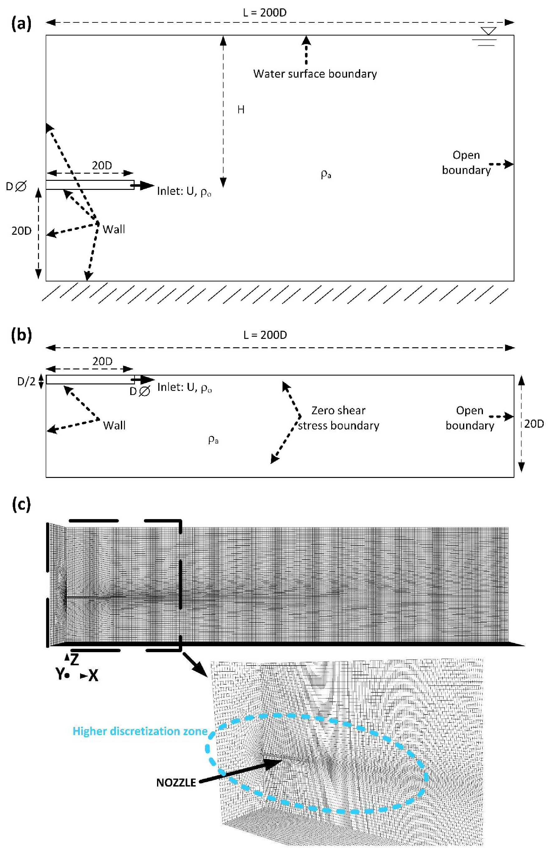
The 3D mesh grid was nondimensionalized by the nozzle diameter with a minimum element size of D/5 near the nozzle and increasing the element size a 10% with a cross-flow size-function until a maximum element size up to D (Figure 2a,b). For the longitudinal advance of the buoyant jet, a constant discretization of D/2 was taken (Figure 2b). This discretization was chosen based on the biunivocal relationship between the mesh discretization and the jet centerline position and dilution to simulate a discharge by means of CFD [32]. The relationship reported that the required grid size close to the single-port has to be at least 1/5 the nozzle diameter to simulate properly the jet entrance. Moreover, the size of the grid elements can be increased using a size function to achieve a maximum element size of 1 diameter close to the contours of the domain. The numerical discretization was conducted by the SIMPLE algorithm (Figure 2c).
In order to assess the model sensitivity to the mesh grid size, three mesh grids were used: (1) coarse grid with 3 × 10⁵ elements, (2) intermediate grid with 6 × 10⁵ elements, and (3) fine grid with 2 × 10⁶ elements. Independently of the simulation case and/or the mesh grid, the numerical discretization was a Crank–Nicholson second order scheme in time and a Van Leer second order scheme for the advection terms. In order to ensure the numerical model stability, a variable time step depending on the turbulent flow was used. The time step started with 10−5 s at the beginning of any simulation and finished with 5 × 10⁻⁴ s at the end of any simulation. The simulation time was 200 s, recording model results every 10−2 s for every numerical test.
The water-free surface (upper boundary) was modelled as a surface with zero shear stress because the variation of water level in the tank was negligible during the duration of the tests. The bottom, wall and nozzle were defined as non-slip closed boundaries. The boundaries in front and parallel to the nozzle were considered as open boundaries under hydrostatic pressure in order to comply with the continuity equation and take out the exceedance mass of the domain. Finally, the initial condition for every simulation case was obtained by applying a first order numerical scheme until achieve a steady state solution (model warm-up).
2.2.3. Setup of the Semiempirical Models
The semiempirical modelling (CORJET and VISJET) was carried out with the same geometry of the CFD modelling (see Figure 2) and taking into account the same physical conditions for both the discharge and the receiving water body. In addition, it should be noted that these models do not interact with the boundaries, so the simulations conclude when the buoyant jet hits the water-free surface.
2.2.4. Performance Metrics of Numerical Modelling
To evaluate the models’ performance, firstly, the coefficient of determination (R2) was calculated as the difference between modelled results and observed values, as expressed in Equation (5). Secondly, the error between both series was assessed using the root-mean square error (RMSE) and the normalized RMSE (NRMSE), displayed in Equations (6) and (7), respectively. Finally, the error between both series was also calculated using the model efficiency (CE), developed by [51] and showed in Equation (8).
where Ri is the i-data of the physical tests, Si is the i-data of the numerical tests, is the average data of the physical tests, and i is the ith value from 1 to N data of the physical tests.
CE ranges between −∞ and 1.0 (1.0 inclusive), with CE = 1 being the optimal value. Values between 0.0 and 1.0 are generally viewed as acceptable levels of performance, whereas values <0.0 indicate that the mean observed value is a better predictor than the simulated value, which indicates unacceptable performance. Depending on the CE value, the comparison is considered acceptable (poor) if CE < 0.4, acceptable (-) if 0.4 ≤ CE < 0.6, acceptable (convenient or good) if 0.6 ≤ CE < 0.8, and acceptable (excellent) if CE ≥ 0.8.
2.3. Zonation of Positively Buoyant Jets
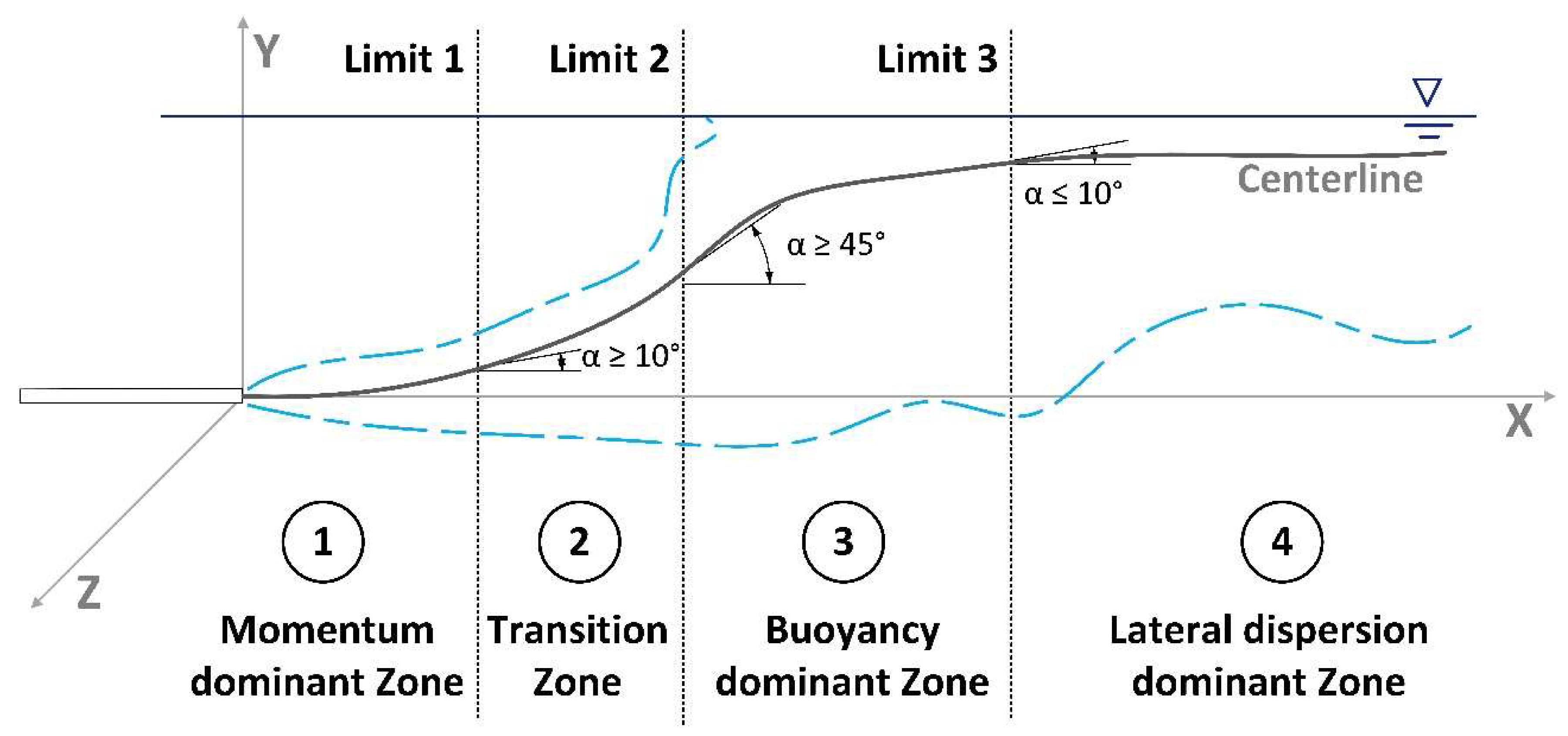
As it was mentioned, the evolution of positively buoyant jets is generally separated into four zones (see Figure 1b,c) according to the competitive relation between momentum and buoyancy [11]. In this work, we proposed a new method to delimitate these zones using the angle (α) shaped by the tangent of the centerline trajectory and the longitudinal axis or X-axis (see Figure 3). α can be seen as an indicator of the relation between momentum and buoyancy.
When introducing a positively buoyant jet in a fluid environment, its behavior is governed by its momentum forces so the jet centerline is parallel to the single-port projection. Thus, the momentum dominant zone can practically be assumed to be up to α equals to 10 degrees because density-driven mechanisms are weak. When the positively buoyant jet goes beyond this angle, it reaches a transition area, where the momentum forces act with a similar magnitude as buoyancy forces. Next, if the angle reaches a value greater than 45 degrees, the force decomposition indicates that the buoyancy forces are greater than momentum forces and, therefore, the jet is in the buoyancy dominant zone. Lastly, when the jet angle is again less than 10 degrees, the positively buoyant jet is considered to advance only by lateral dispersion, entering in the so-called lateral dispersion dominant zone.
The Limit 1 is defined when α is equal or greater than 10 degrees, i.e., buoyancy begins to be significant. It should be noted that lateral mixing of the jet with the receiving water starts to decrease (shear layer mixing). This effect is an indicator of the transition between the dominance of momentum forces with respect to buoyancy. Next, the Limit 2 is established when α is equal or greater than 45 degrees because it is the turning point where buoyancy is stronger than momentum. It should be noted that 45 degrees marks the point where the forces in the horizontal direction (momentum forces) are smaller than the forces in the vertical direction (buoyancy forces) according to the force decomposition.
3. Results
3.1. Physycal Modelling
3.1.1. PIV Measurements
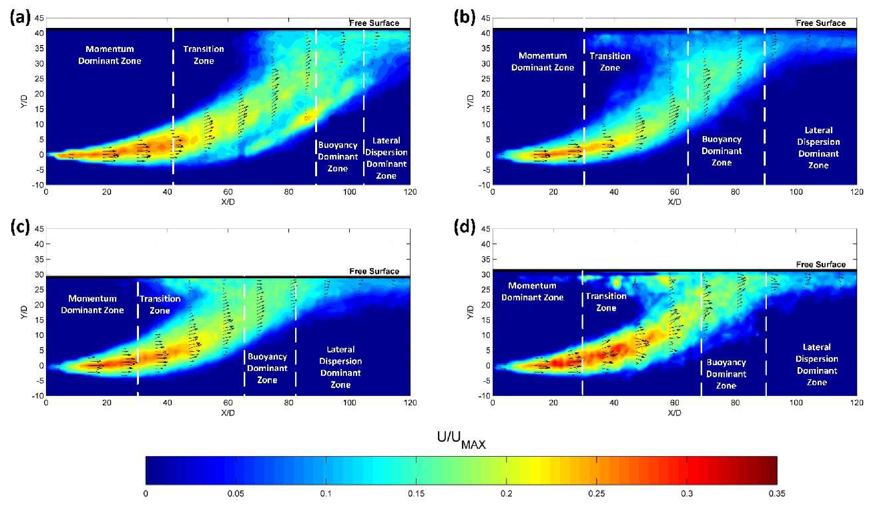
Figure 4 shows the dimensionless velocity (U/UMAX) in a longitudinal view of the positively buoyant jet advance at the nozzle XY plane for the tests V1 (a), V2 (b), V3 (c) and V4 (d).
All physical tests presented an evolution dominated by momentum for x/D ranging between 29 (V2) and 41.5 (V1). The transition zone was located between 29 ≤ x/D < 65 for V2 and 41.5 ≤ x/D < 90 for V1. Moreover, the buoyant jet evolution was dominated by buoyancy in the region 65 ≤ x/D < 91 for V2 and 90 ≤ x/D < 104 for V1. Independently of the physical test, the buoyant jet evolution shows, for x/D ≥ 104, a movement parallel to the free surface, i.e., entering in the lateral dispersion dominant zone. From these results, we can highlight (1) the higher the flow discharge, the greater the extension of Zones 1 and 2; (2) the higher the density gradient between the discharge and the receiving water body, the greater the extension of Zone 3; and (3) the higher the water depth of the receiving water body, the greater the extension on all zones.
3.1.2. LIF Measurements
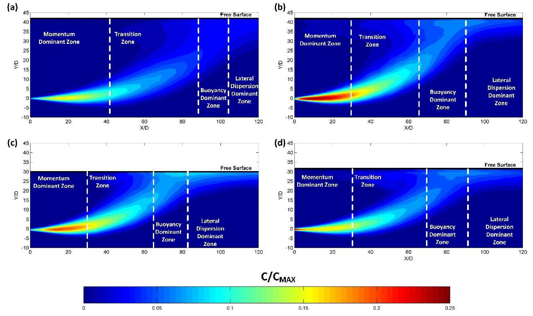
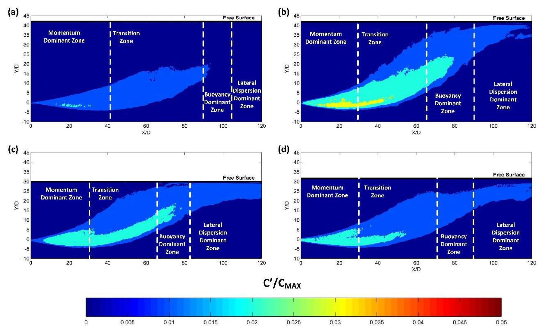
Figure 5 and Figure 6 show the dimensionless concentrations (C/CMAX) and the dimensionless fluctuations of the concentration (C’/CMAX) in a longitudinal view of the positively buoyant jet advance at the nozzle XY plane for the tests V1 (a), V2 (b), V3 (c) and V4 (d), respectively.
Figure 5 shows, in all cases, the concentration was reduced to 15%–10% of the initial concentration (Co) at Limit 1. Between X/D = 0 and X/D = 20, the test results presented outliers since the rhodamine concentrations used showed a saturation in their emission values and could not provide reliable results in this area. Next, the concentration was reduced to values of the order or less than 5% of Co at the Limit 2. However, in the physical test V2, the development of the buoyant jet generates a higher concentration due to the relationship between the jet momentum and the water depth until it hits the water-free surface. As can be seen in Figure 6, the fluctuation values are less than 1% of CMAX in all the zones of the buoyant jet. Nonetheless, these fluctuations can present values corresponding to 2% of CMAX in the central area of the buoyant jet before reaching the Zone 3, independently of the physical test.
3.2. Numerical Modelling
3.2.1. Setup of the Computational Fluid Dynamics Model
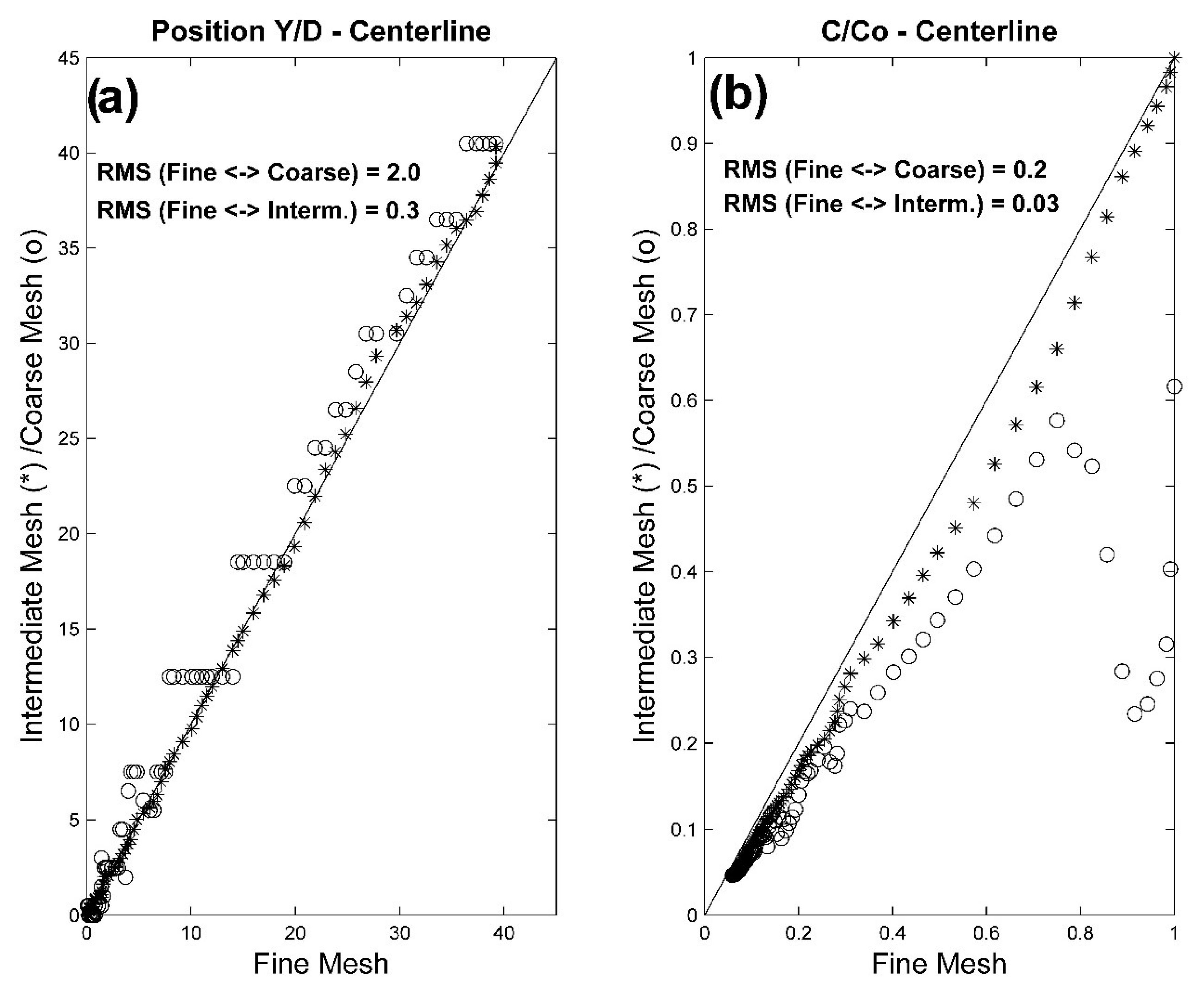
In order to compare the results with the three grid resolutions for OpenFOAM, Figure 7 shows a scatter plot of the centerline trajectory (Figure 7a) in dimensionless positions (X/D and Y/D), and a scatter plot of the C/CMAX along the centerline (Figure 7b) for the fine grid versus the intermediate grid (circle markers), and the fine grid versus the coarse grid (star markers), respectively.
When the centerline trajectory of the fine grid was compared with the coarse and intermediate grids, the RMS was 2.0 and 0.3, respectively. For the comparison of the C/CMAX along the centerline, the coarse and intermediate grids displayed a RMS of 0.2 and 0.03, respectively. Furthermore, the simulation time was 72 h, 9.5 h and 3 h for the fine, intermediate and coarse grids, respectively. These results support the use of the intermediate grid due to the trade-off between computational time and model accuracy.
3.2.2. Performance of Numerical Models
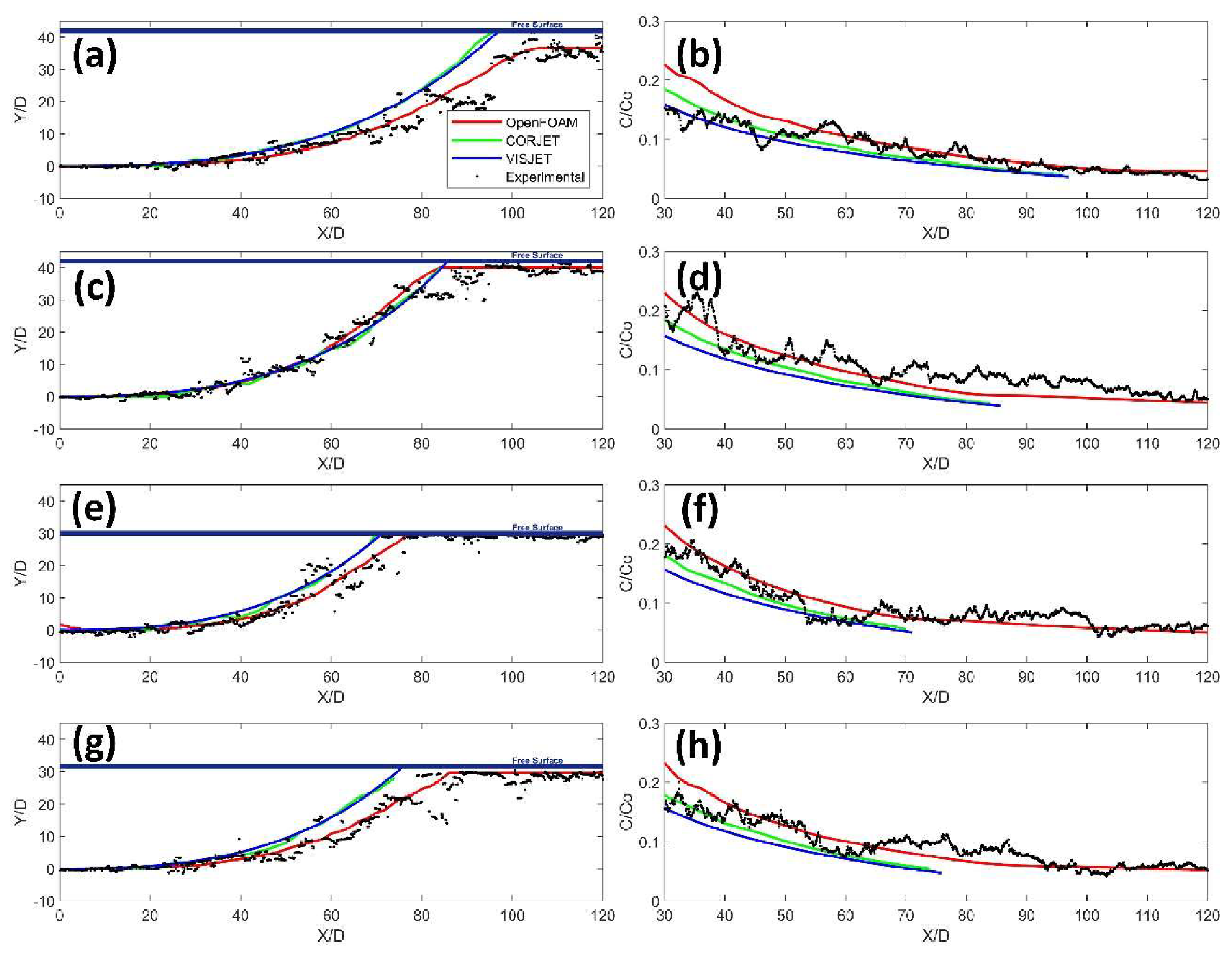
Figure 8 displays the comparison between the physical results (black dots) and the numerical results obtained with CORJET (green line), VISJET (blue line) and OpenFOAM (red line) of the centerline trajectory (left panels) in dimensionless positions (X/D and Y/D) and the C/CMAX along the centerline (right panels) for the tests V1 (a, b), V2 (c, d), V3 (e, f) and V4 (g, h).
As can be seen in Figure 8, the two semiempirical models shown a similar result. It is noteworthy to point out that these models did not need any boundary conditions but an initial condition for the ambient density (calculated with the UNESCO equation from temperature and salinity). From X/D = 20, semiempirical models represented a tendency to decrease in concentration, as seen in the physical tests, but overestimated the dilution by 50% when the models reached the water-free surface and finished their calculation. Regarding OpenFOAM results, it can be seen that CFD simulation provided better results than semiempirical models.
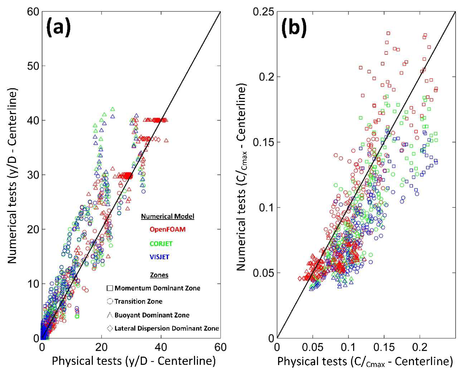
In order to assess the performance of the numerical models to reproduce the physical tests, R2, RMSE, NRMSE, and CE were calculated (Table 2). Figure 9 displays a scatter plot of the centerline trajectory (Figure 9a) in dimensionless positions (X/D and Y/D), and a scatter plot of the C/CMAX along the centerline (Figure 9b) for the physical results versus the numerical results obtained with CORJET (green markers), VISJET (blue markers) and OpenFOAM (red markers) for the momentum dominant zone (square markers), the momentum to buoyancy transition zone (circle markers), the buoyancy dominant zone (triangle markers), and the lateral dispersion dominant zone (diamond markers), respectively.
For both the trajectory and C/CMAX, R2 values were above 0.8 for OpenFOAM. Moreover, CE values for OpenFOAM were considered as excellent (CE > 0.8) and good (CE > 0.6) for centerline position and dilution along the centerline, respectively. On the other hand, this metric shows semiempirical models provided good results (CE > 0.6) for the centerline position but their results were poor (CE < 0.4) in defining the dilution of a positively buoyant jet.
The three considered models provided good agreement with physical tests for the centerline position. Semiempirical models CORJET and VISJET obtained a CE value of 0.78 and 0.79 (classified as good), respectively, (Table 2) and the CE value for OpenFOAM was classed as excellent, being CE = 0.98. The lower NRMSE was obtained by OpenFOAM with a value of 4.62%, better than the approximately 12% obtained by semiempirical models. In terms of R2, the three models obtained a very high value (>0.87), being especially high for OpenFOAM (0.98).
The analysis of the dilution shown the best results were obtained by OpenFOAM, with a CE of 0.64, a NRMSE of 12% and a R2 greater than 0.8. However, in the case of semiempirical models, the CORJET obtained a CE of 0.45 (acceptable result) and the VISJET of 0.37 (poor result), a NRMSE of 16% and 20%, respectively, and a R2 less than 0.8 for both semiempirical models.
3.3. Zonation of Positively Buoyant Jets
The zone limits of the positively buoyant jet for the four physical tests (V1 to V4) were determined from the experimental, OpenFOAM, CORJET, and VISJET data and summarized in Table 3. In order to assess the performance of the numerical models to define the limits of positively buoyant jet zones, the RMSE, and NRMSE were calculated in Table 4. It should be noted Limits 1, 2 and 3 are defined by α value of 10 degrees (limit of separation between the momentum and transition zone), 45 degrees (limit between the transition zone and the buoyancy dominant zone) and again 10 degrees (limit of the zone where the flow pattern is dominated by lateral dispersion), respectively.
According to the experimental data, Limit 2 was reached at a distance 2.14 times the Limit 1. In the case of numerical models, this distance was 2.15, 2.43 and 2.51 times the Limit 1 for OpenFOAM, CORJET and VISJET models, respectively. Next, Limit 3 was reached at 1.2 times the Limit 2 for both experimental data and the OpenFOAM numerical model. In addition, both the physical tests and the results obtained with OpenFOAM found that the relationship between the Limit 3 and Limit 1 was 2.7. All these values were the average data of the four tests.
As shown in Table 4, the OpenFOAM numerical model best represented the evolution of the positively buoyant jet in all the proposed zones until it reached the lateral dispersion dominant zone (Zone 4). In the Limits 1 and 2, the OpenFOAM model had an RMSE approximately five times lower than the semiempirical models CORJET and VISJET. In the case of Limit 3, the OpenFOAM values cannot be compared with the semiempirical models since they cannot give results when the buoyant jet advances to the lateral dispersion dominant zone.
When comparing the zonation Limits calculated by the experimental data, the NRMSE shows that the OpenFOAM error was less than 7% in both Limits 1 and 2. For the case of CORJET, the differences were 39% and 22.6% in Limits 1 and 2, respectively, and 45.6% and 18.2% for the case of VISJET in those limits. As can be seen, the models are capable of giving results with less standardized error with the jet advance up to the moment of impact with the water-free surface.
4. Discussion
4.1. Physycal Modelling
Physical tests have provided similar results to previous studies along the Zones 1 and 2 of positively buoyant jets [7,8,11,58].
A fundamental aspect of buoyant jets is the relationship between the dispersion of mass and energy (velocity) related to its centerline. This relationship (λ) is defined throughout the ratio between the maximum dimensionless concentrations CMaxi and velocities UMaxi in a selected profile (see Equation (9)). According to [59], the value of λ follows a non-linear pattern in the centerline advance along the longitudinal axis.
For instance, λ was obtained for the profiles X/D = 20, X/D = 60, X/D = 80 and X/D = 110, which are representative of the four different zones in the evolution of positively buoyant jets, showing an average value for the four physical tests of 0.73, 0.57, 0.51 and 0.60, respectively. The highest values of λ were located inside the momentum dominant zone (Zone 1) because this zone includes the most energetic vortices. λ values started to decrease in the transition zone (Zone 2) due to the reduction of the turbulent energy. In the Zone 3, λ continued decreasing because the turbulent energy is weaker. In the Zone 4, λ values increased due to the vortices destruction and the advance by dispersion. Finally, λ reached a constant value when the turbulent wake was fully developed in the lateral dispersion dominant zone (Zone 4).
From the Zone 3 until Zone 4, the positively buoyant jet was not axisymmetric because the water-free surface behaved like a wall. Therefore, the buoyant jet only presents dispersion in the half bottom of its volume. This fact reduces the differences between energy and mass dispersion (half dispersion of mass and energy) so the net values of both were more similar, considering that λ is less than one in all profiles that cut the advance of the buoyant jet. These results agree with [59] as the higher stretching vortex processes were in the first part of the buoyant jet evolution (increasing mixing processes), then they diminished in the impact zone with the water-free surface (dominated by advection) and then lightly increased with the turbulent wake.
4.2. Numerical Modelling
As shown in Figure 8, semiempirical models do not allow calculating the jet trajectory and dilution in the Zone 4. Due to their non-interaction with the water-free surface, semiempirical models do not change their trajectory when approaching it. As a consequence, semiempirical models presented a shorter distance of the impact point with the water-free surface than the experimental data or the CFD model. On the contrary, CFD models provide results in a continuous mode from the Zone 1 until the Zone 4.
Numerical models enable accurate results with less standardized error for the evolution of positively buoyant jets until the Limit 2. In the case of the OpenFOAM model, the only one capable of obtaining Limit 3, it can be seen that Limit 3 has a standard error that doubles the value obtained in the previous limits. The increase of the error in this area is due to the buoyant jet mechanics is governed by diffusion and, therefore, it is more sensitive to numerical diffusion phenomena, which were less appreciable in the areas where the buoyant jet moved either by momentum or by buoyancy gradients.
Overall, the obtained results suggest that semiempirical models can provide results in a range error of ±50% and CFD models obtain much better results for both centerline position and dilution in the four zones of a positively buoyant jet. Taking into account the accuracy of numerical models in every zone, model results suggest the use of semiempirical models for only calculations in Zones 1 and 2 while CFD models are applicable for anyone. However, depending on the case study, the high computational costs of CFD models should be always considered for the model selection due to the trade-off between computational time and model accuracy. Accordingly, CFD models could be used in further work to analyze the zonation of other buoyant jet configurations without laboratory testing, meanwhile, semiempirical models could not be used as additional information generators due to the displayed errors.
4.3. Zonation of Positively Buoyant Jets
The buoyant jets have been delimited by length scales based on physical modelling [11,35,36,37]. However, in many cases, these length scales cannot be calculated with numerical modelling. This work tries to overcome these constraints by proposing a simple indicator, α, able to delimitate the evolution of positively buoyant jets from physical and numerical model results. Thus, classical methods based on the dimensional analysis of variables may prescribe uncertainty about the location of the different zones because the classification use length scales build through linear fits with an error higher than 30% [38].
The Limit 1 could correspond to the momentum length scale (LM) proposed by [11] because both mark the limit of momentum dominant zone-based characteristics (single-port diameter, momentum and buoyancy). The obtained values were very similar to those obtained with the proposed methodology. Regarding the Limit 2, the classical length scales do not include a specific methodology to obtain it. For instance, the calculation of the buoyancy length scale (LB), proposed by [11], is diffused and constrained to the existence of stratification in the receiving medium. Finally, according to the Roberts experiments [35,36,37], the Limit 3 is obtained when the vertical concentration profile in the layer where the buoyant jet is progressing presents longitudinal variations lower than 5%. This calculation was in line with the lengths obtained by the proposed method for the Limit 3. Table 5 shows the values of these scales for the laboratory tests.
As can be seen in Table 5, the values of Limit 1 obtained by LM are closer to the semiempirical models results than the laboratory test data, displaying an error of 44% compared with physical test data and displaying more error than modelling errors obtained by means of OpenFOAM (error value of 6.4% compared with test data). In the case of Limit 2, LB could not be calculated because the environment did not present stratification. Finally, the point marked by [35,36,37], as Limit 3, shows a variation of 25% compared with the physical tests; this variation is greater than the variation for OpenFOAM (a variation for the Limit 3 location of 11.9%).
5. Conclusions
A new method to delimitate the four characteristic zones of positively buoyant jets interacting with the water-free surface was proposed using the angle (α) shaped by the tangent of the centerline trajectory and the longitudinal axis. These zones are (1) momentum dominant zone (jet-like), (2) momentum to buoyancy transition zone (jet to plume), (3) buoyancy dominant zone (plume-like), and (4) lateral dispersion dominant zone. The validation of the proposed method was tested by the results obtained with physical and numerical modelling. The proposed method could be imposed as a more general strategy when analyzing the different zones in which the evolution of positively buoyant jets can be separated because it can be always calculated by physical and numerical model results.
The proposed parameter α can be seen as an indicator of the relation between momentum and buoyancy. The Limit 1 (Zone 1 to 2) is defined when α is equal or greater than 10 degrees, i.e., buoyancy begins to be significant. Next, the Limit 2 (Zone 2 to 3) is established when α is equal or greater than 45 degrees because this is the turning point where buoyancy becomes stronger than momentum. Finally, the Limit 3 (Zone 3 to 4) is specified when α is again equal or lower than 10 degrees, i.e., the buoyant jet evolution is again parallel to the longitudinal axis (X-axis) and the water-free surface.
Furthermore, the evolution of positively buoyant jets was studied with non-intrusive techniques (PIV and LIF) by analyzing four physical tests in the four characteristic zones. The coupled analysis of PIV and LIF shows that the dispersion of mass (concentrations) is always greater than the dispersion of energy (velocity) during the evolution of positively buoyant jets.
Regarding numerical modelling, on the one hand, the semiempirical models (CORJET and VISJET) for the study of positively buoyant jets underestimate the advance of the jets up to their impact with the water-free surface, where they end the calculation. In turn, these numerical models overestimate the actual dilution reached by positively buoyant jets, especially close to the impact zone. On the other hand, the CFD model (OpenFOAM) for the study of positively buoyant jets was able to faithfully reproduce the behavior of the buoyant jet for all the proposed zones according to the physical results. CFD can also avoid the simplifications made by semiempirical models for the study of jet dynamics (trajectory and dilution). In addition, CFD models are able to consider all such complexity in relation to the geometry of the diffusers and the receiving water body. The use of this technique allows, in a single calculation, results to be obtained in all the zones.
The application of the proposed method by using numerical modelling has shown that the semiempirical models underestimate the distance of the limits for the different zones proposed in the methodology. The comparison of the laboratory test data with the OpenFOAM results showed an error of 6.4% and 5.4% in the definition of Limits 1 and 2, respectively. Moreover, a comparison with semiempirical models showed higher errors, with error values of 39% and 22.6% in the case of CORJET and 45.6% and 18.2% in the case of VISJET for the location of the Limits 1 and 2, respectively. It should be noted that the semiempirical models cannot offer information on Limit 3. In contrast, the OpenFOAM model displayed an error value of 11.9% for Limit 3 with respect to the laboratory tests.
Therefore, CFD models increases the understanding about the evolution of positively buoyant jets in the aquatic medium and will facilitate the improvement of the discharge designing process. This fact could be a starting point for their use as information/data providers, i.e., a virtual laboratory, in order to generate better semiempirical models or advanced statistical models based on artificial intelligence techniques, enabling the analysis of new discharge system configurations without large computational costs or large physical modelling costs. Finally, CFD model results might be used to develop an abacus to gauge the influence of key parameters on the initial dilution, location, width and thickness of positively buoyant jets in order to predict the behavior of any discharge in the near-field and couple this with far-field models.
Author Contributions
Conceptualization, J.G.-A.; methodology, J G.-A., J.F.B. and A.G.; investigation, J.G.-A. and J.F.B.; data curation, J.G.-A.; writing—original draft preparation, J.G.-A. and J.F.B.; writing—review and editing, J.G.-A., and J.F.B.; visualization, J.G.-A. and J.F.B.; funding acquisition, A.G. All authors have read and agreed to the published version of the manuscript.
Funding
The work described in this paper is part of a research project financed by the VI National Plan (2008–2012) for Research in Science and Technological Innovation of the Spanish Government (VERTIZE CTM2012-32538).
Acknowledgments
The authors would like to thank the editor and reviewers for their suggestions that have improved this article.
Conflicts of Interest
The authors declare no conflict of interest.
References
- Roose, P.; Brinkman, U.A.T. Monitoring Organic Microcontaminants in the Marine Environment: Principles, Programmes and Progress. TrAC Trends Anal. Chem. 2005, 24, 897–926. [Google Scholar] [CrossRef]
- Bárcena, J.F.; Claramunt, I.; García-Alba, J.; Pérez, M.L.; García, A. A Method to Assess the Evolution and Recovery of Heavy Metal Pollution in Estuarine Sediments: Past History, Present Situation and Future Perspectives. Mar. Pollut. Bull. 2017, 124, 421–434. [Google Scholar] [CrossRef] [PubMed]
- Demchenko, N.; He, C.; Rao, Y.R.; Valipour, R. Surface River Plume in a Large Lake under Wind Forcing: Observations and Laboratory Experiments. J. Hydrol. 2017, 553, 1–12. [Google Scholar] [CrossRef]
- Bárcena, J.F.; Gómez, A.G.; García, A.; Álvarez, C.; Juanes, J.A. Quantifying and Mapping the Vulnerability of Estuaries to Point-Source Pollution Using a Multi-Metric Assessment: The Estuarine Vulnerability Index (EVI). Ecol. Indic. 2017, 76, 159–169. [Google Scholar] [CrossRef]
- García, J.; Álvarez, C.; García, A.; Revilla, J.; Juanes, J. Study of a Thermal Brine Discharge Using a 3D Model. In Environmental Hydraulics, Two Volume Set; CRC Press: London, UK, 2010; Volume 1, pp. 553–558. [Google Scholar] [CrossRef]
- Cushman-Roisin, B.; Gačić, M.; Poulain, P.-M.; Artegiani, A. Physical Oceanography of the Adriatic Sea; Springer: Dordrecht, The Netherlands, 2001. [Google Scholar] [CrossRef]
- Koh, R.C.Y.; Brooks, N.H. Fluid Mechanics of Waste-Water Disposal in the Ocean. Annu. Rev. Fluid Mech. 1975, 7, 187–211. [Google Scholar] [CrossRef] [Green Version]
- Ungate, C.D.; Harleman, D.R.F.; Jirka, G.H. Stability and Mixing of Submerged Turbulent Jets at Low Reynolds Numbers; MIT Energy Lab: Cambridge, UK, 1975; Available online: https://dspace.mit.edu/handle/1721.1/27517 (accessed on 23 January 2020).
- Fischer, H.B. Mixing in Inland and Coastal Waters; Academic Press: San Diego, CA, USA, 1979. [Google Scholar] [CrossRef]
- Wallace, R.B.; Wright, S.J. Spreading Layer of Two-Dimensional Buoyant Jet. J. Hydraul. Eng. 1984, 110, 813–828. [Google Scholar] [CrossRef]
- Jirka, G.H.; Domeker, R.L. Hydrodynamic Classification of Submerged Single-Port Discharges. J. Hydraul. Eng. 1991, 117, 1095–1112. [Google Scholar] [CrossRef]
- Lee, J.H.W.; Cheung, V. Generalized Lagrangian Model for Buoyant Jets in Current. J. Environ. Eng. 1990, 116, 1085–1106. [Google Scholar] [CrossRef]
- Akar, P.J.; Jirka, G.H. Buoyant Spreading Processes in Pollutant Transport and Mixing Part 1: Lateral Spreading with Ambient Current Advection. J. Hydraul. Res. 1994, 32, 815–831. [Google Scholar] [CrossRef]
- Alba, J.G.; Gómez, A.G.; del Barrio Fernández, P.; Gómez, A.G.; Álvarez Díaz, C. Hydrodynamic Modelling of a Regulated Mediterranean Coastal Lagoon, the Albufera of Valencia (Spain). J. Hydroinform. 2014, 16, 1062–1076. [Google Scholar] [CrossRef] [Green Version]
- Bárcena, J.F.; García-Alba, J.; García, A.; Álvarez, C. Analysis of Stratification Patterns in River-Influenced Mesotidal and Macrotidal Estuaries Using 3D Hydrodynamic Modelling and K-Means Clustering. Estuar. Coast. Shelf Sci. 2016, 181, 1–13. [Google Scholar] [CrossRef]
- Gogineni, S.; Goss, L.; Roquemore, M. Manipulation of a Jet in a Cross Flow. Exp. Therm. Fluid Sci. 1998, 16, 209–219. [Google Scholar] [CrossRef]
- Pantzlaff, L.; Lueptow, R.M. Transient Positively and Negatively Buoyant Turbulent Round Jets. Exp. Fluids 1999, 27, 117–125. [Google Scholar] [CrossRef]
- Li, C.-T.; Chang, K.-C.; Wang, M.-R. PIV Measurements of Turbulent Flow in Planar Mixing Layer. Exp. Therm. Fluid Sci. 2009, 33, 527–537. [Google Scholar] [CrossRef]
- Wen, Q.; Kim, H.D.; Liu, Y.Z.; Kim, K.C. Dynamic Structures of a Submerged Jet Interacting with a Free Surface. Exp. Therm. Fluid Sci. 2014, 57, 396–406. [Google Scholar] [CrossRef]
- González-Espinosa, A.; Buchmann, N.; Lozano, A.; Soria, J. Time-Resolved Stereo PIV Measurements in the Far-Field of a Turbulent Zero-Net-Mass-Flux Jet. Exp. Therm. Fluid Sci. 2014, 57, 111–120. [Google Scholar] [CrossRef]
- Tian, X.; Roberts, P.J.W.; Daviero, G.J. Marine Wastewater Discharges from Multiport Diffusers. I: Unstratified Stationary Water. J. Hydraul. Eng. 2004, 130, 1137–1146. [Google Scholar] [CrossRef]
- Tian, X.; Roberts, P.J.W.; Daviero, G.J. Marine Wastewater Discharges from Multiport Diffusers. II: Unstratified Flowing Water. J. Hydraul. Eng. 2004, 130, 1147–1155. [Google Scholar] [CrossRef]
- Daviero, G.J.; Roberts, P.J. Marine Wastewater Discharges from Multiport Diffusers. III: Stratified Stationary Water. J. Hydraul. Eng. 2006, 132, 404–410. [Google Scholar] [CrossRef]
- Tian, X.; Roberts, P.J.; Daviero, G.J. Marine Wastewater Discharges from Multiport Diffusers. IV: Stratified Flowing Water. J. Hydraul. Eng. 2006, 132, 411–419. [Google Scholar] [CrossRef]
- Kikkert, G.A.; Davidson, M.J.; Nokes, R.I. Buoyant Jets with Three-Dimensional Trajectories. J. Hydraul. Res. 2010, 48, 292–301. [Google Scholar] [CrossRef]
- Kawanabe, H.; Kondo, C.; Kohori, S.; Shioji, M. Simultaneous Measurements of Velocity and Scalar Fields in a Turbulent Jet Using PIV and LIF. J. Environ. Eng. 2010, 5, 231–239. [Google Scholar] [CrossRef] [Green Version]
- Xu, D.; Chen, J. Experimental Study of Stratified Jet by Simultaneous Measurements of Velocity and Density Fields. Exp. Fluids 2012, 53, 145–162. [Google Scholar] [CrossRef]
- Grafsrønningen, S.; Jensen, A. Simultaneous PIV/LIF Measurements of a Transitional Buoyant Plume above a Horizontal Cylinder. Int. J. Heat Mass Transf. 2012, 55, 4195–4206. [Google Scholar] [CrossRef]
- Siddiqui, M.I.; Munir, S.; Heikal, M.R.; de Sercey, G.; Aziz, A.R.A.; Dass, S.C. Simultaneous Velocity Measurements and the Coupling Effect of the Liquid and Gas Phases in Slug Flow Using PIV–LIF Technique. J. Vis. 2016, 19, 103–114. [Google Scholar] [CrossRef] [Green Version]
- Wang, H.; Wing-Keung Law, A. Second-Order Integral Model for a Round Turbulent Buoyant Jet. J. Fluid Mech. 2002, 459, 397–428. [Google Scholar] [CrossRef]
- Tang, H.S.; Paik, J.; Sotiropoulos, F.; Khangaonkar, T. Three-Dimensional Numerical Modeling of Initial Mixing of Thermal Discharges at Real-Life Configurations. J. Hydraul. Eng. 2008, 134, 1210–1224. [Google Scholar] [CrossRef] [Green Version]
- García Alba, J. Estudio de Chorros Turbulentos Con Modelos Cfd: Aplicación En El Diseño de Emisarios Submarinos; Universidad de Cantabria: Santander, Spain, 2011. [Google Scholar]
- Doneker, R.L.; Jirka, G.H. Expert Systems for Mixing-Zone Analysis and Design of Pollutant Discharges. J. Water Resour. Plan. Manag. 1991, 117, 679–697. [Google Scholar] [CrossRef]
- Lee, J.H.W.; Cheung, V.W.L. Inclined Plane Buoyant Jet in Stratified Fluid. J. Hydraul. Eng. 1986, 112, 580–589. [Google Scholar] [CrossRef]
- Roberts, P.J.W.; Snyder, W.H.; Baumgartner, D.J. Ocean Outfalls. I: Submerged Wastefield Formation. J. Hydraul. Eng. 1989, 115, 1–25. [Google Scholar] [CrossRef]
- Roberts, P.J.W.; Snyder, W.H.; Baumgartner, D.J. Ocean Outfalls. II: Spatial Evolution of Submerged Wastefield. J. Hydraul. Eng. 1989, 115, 26–48. [Google Scholar] [CrossRef]
- Roberts, P.J.W.; Snyder, W.H.; Baumgartner, D.J. Ocean Outfalls. III: Effect of Diffuser Design on Submerged Wastefield. J. Hydraul. Eng. 1989, 115, 49–70. [Google Scholar] [CrossRef]
- Palomar, P.; Lara, J.L.; Losada, I.J.; Rodrigo, M.; Alvárez, A. Near Field Brine Discharge Modelling Part 1: Analysis of Commercial Tools. Desalination 2012, 290, 14–27. [Google Scholar] [CrossRef]
- Crimaldi, J.P. Planar Laser Induced Fluorescence in Aqueous Flows. Exp. Fluids 2008, 44, 851–863. [Google Scholar] [CrossRef]
- Martin, J.E.; García, M.H. Combined PIV/PLIF Measurements of a Steady Density Current Front. Exp. Fluids 2009, 46, 265–276. [Google Scholar] [CrossRef]
- Liao, Q.; Cowen, E.A. Relative Dispersion of a Scalar Plume in a Turbulent Boundary Layer. J. Fluid Mech. 2010, 661, 412–445. [Google Scholar] [CrossRef]
- Pérez-Díaz, B.; Palomar, P.; Castanedo, S.; Álvarez, A. PIV-PLIF Characterization of Nonconfined Saline Density Currents under Different Flow Conditions. J. Hydraul. Eng. 2018, 144, 04018063. [Google Scholar] [CrossRef]
- Willert, C. The Fully Digital Evaluation of Photographic PIV Recordings. Appl. Sci. Res. 1996, 56, 79–102. [Google Scholar] [CrossRef]
- Sarpkaya, T. Vorticity, Free Surface, and Surfactants. Annu. Rev. Fluid Mech. 1996, 28, 83–128. [Google Scholar] [CrossRef]
- Ferrier, A.J.; Funk, D.R.; Roberts, P.J.W. Application of Optical Techniques to the Study of Plumes in Stratified Fluids. Dyn. Atmos. Ocean. 1993, 20, 155–183. [Google Scholar] [CrossRef]
- UNESCO. The International Thermodynamic Equation of Seawater-2010: Calculation and Use of Thermodynamic Properties Intergovernmental Oceanographic Commission; UNESCO: Paris, France, 2015; Available online: https://unesdoc.unesco.org/ark:/48223/pf0000193020 (accessed on 4 February 2020).
- Jirka, G.H. Integral Model for Turbulent Buoyant Jets in Unbounded Stratified Flows. Part I: Single Round Jet. Environ. Fluid Mech. 2004, 4, 1–56. [Google Scholar] [CrossRef]
- Jirka, G.H. Integral Model for Turbulent Buoyant Jets in Unbounded Stratified Flows Part 2: Plane Jet Dynamics Resulting from Multiport Diffuser Jets. Environ. Fluid Mech. 2006, 6, 43–100. [Google Scholar] [CrossRef]
- Jirka, G.H. Buoyant Surface Discharges into Water Bodies. II: Jet Integral Model. J. Hydraul. Eng. 2007, 133, 1021–1036. [Google Scholar] [CrossRef]
- Higuera, P.; Lara, J.L.; Losada, I.J. Realistic Wave Generation and Active Wave Absorption for Navier–Stokes Models. Coast. Eng. 2013, 71, 102–118. [Google Scholar] [CrossRef]
- Nash, J.E.; Sutcliffe, J.V. River Flow Forecasting through Conceptual Models Part I—A Discussion of Principles. J. Hydrol. 1970, 10, 282–290. [Google Scholar] [CrossRef]
- Moriasi, D.N.; Arnold, J.G.; Van Liew, M.W.; Bingner, R.L.; Harmel, R.D.; Veith, T.L. Model Evaluation Guidelines for Systematic Quantification of Accuracy in Watershed Simulations. Trans. ASABE 2007, 50, 885–900. [Google Scholar] [CrossRef]
- García Alba, J.; Gómez, A.G.; Tinoco López, R.O.; Sámano Celorio, M.L.; García Gómez, A.; Juanes, J.A. A 3-D Model to Analyze Environmental Effects of Dredging Operations—Application to the Port of Marin, Spain. Adv. Geosci. 2014, 39, 95–99. [Google Scholar] [CrossRef] [Green Version]
- Gómez, A.G.; García Alba, J.; Puente, A.; Juanes, J.A. Environmental Risk Assessment of Dredging Processes—Application to Marin Harbour (NW Spain). Adv. Geosci. 2014, 39, 101–106. [Google Scholar] [CrossRef] [Green Version]
- García-Alba, J.; Bárcena, J.F.; Ugarteburu, C.; García, A. Artificial Neural Networks as Emulators of Process-Based Models to Analyse Bathing Water Quality in Estuaries. Water Res. 2019, 150, 283–295. [Google Scholar] [CrossRef]
- Zapata, C.; Puente, A.; García, A.; García-Alba, J.; Espinoza, J. The Use of Hydrodynamic Models in the Determination of the Chart Datum Shape in a Tropical Estuary. Water 2019, 11, 902. [Google Scholar] [CrossRef] [Green Version]
- Servat, E.; Dezetter, A. Selection of Calibration Objective Fonctions in the Context of Rainfall-Ronoff Modelling in a Sudanese Savannah Area. Hydrol. Sci. J. 1991, 36, 307–330. [Google Scholar] [CrossRef]
- Sobey, R.J.; Johnston, A.J.; Keane, R.D. Horizontal Round Buoyant Jet in Shallow Water. J. Hydraul. Eng. 1988, 114, 910–929. [Google Scholar] [CrossRef]
- Kida, S.; Takaoka, M.; Hussain, F. Collision of Two Vortex Rings. J. Fluid Mech. 1991, 230, 583–646. [Google Scholar] [CrossRef]
Figure 1.
Schematic diagram and photography of the physical model (a), profile view of a preliminary test (b), and plane view of a preliminary test (c).
Figure 1.
Schematic diagram and photography of the physical model (a), profile view of a preliminary test (b), and plane view of a preliminary test (c).

Figure 2.
Mesh grid scheme for the simulation of a jet in a stagnant medium interacting with the water-free surface by means of the computational fluid dynamics (CFD) model: (a) profile view, (b) plan view, and (c) example of CFD mesh grid.
Figure 2.
Mesh grid scheme for the simulation of a jet in a stagnant medium interacting with the water-free surface by means of the computational fluid dynamics (CFD) model: (a) profile view, (b) plan view, and (c) example of CFD mesh grid.

Figure 3.
Proposed zonation of positively buoyant jets using the angle (α) shaped by the tangent of the centerline trajectory and the longitudinal axis (X-axis).
Figure 3.
Proposed zonation of positively buoyant jets using the angle (α) shaped by the tangent of the centerline trajectory and the longitudinal axis (X-axis).

Figure 4.
Dimensionless time-averaged velocities (U/UMAX) in a longitudinal view of the positively buoyant jet advance at the nozzle XY plane for the physical tests V1 (a), V2 (b), V3 (c), and V4 (d).
Figure 4.
Dimensionless time-averaged velocities (U/UMAX) in a longitudinal view of the positively buoyant jet advance at the nozzle XY plane for the physical tests V1 (a), V2 (b), V3 (c), and V4 (d).

Figure 5.
Dimensionless time-averaged concentrations (C/CMAX) in a longitudinal view of the positively buoyant jet advance at the nozzle XY plane for the physical tests V1 (a), V2 (b), V3 (c), and V4 (d).
Figure 5.
Dimensionless time-averaged concentrations (C/CMAX) in a longitudinal view of the positively buoyant jet advance at the nozzle XY plane for the physical tests V1 (a), V2 (b), V3 (c), and V4 (d).

Figure 6.
Dimensionless time-averaged fluctuations of the concentration (C’/CMAX) in a longitudinal view of the positively buoyant jet advance at the nozzle XY plane for the physical tests V1 (a), V2 (b), V3 (c), and V4 (d).
Figure 6.
Dimensionless time-averaged fluctuations of the concentration (C’/CMAX) in a longitudinal view of the positively buoyant jet advance at the nozzle XY plane for the physical tests V1 (a), V2 (b), V3 (c), and V4 (d).

Figure 7.
(a) Scatter plot of the centerline trajectory in dimensionless positions (X/D and Y/D), and (b) scatter plot of the C/CMAX along the centerline for the fine grid versus the medium grid (circle markers), and the fine grid versus the coarse grid (star markers). <-> indicates the used grids for the RMS calculation.

Figure 8.
Comparison of the physical results (black dots) versus the numerical results obtained with CORJET (green line), VISJET (blue line) and Open Field Operation And Manipulation model (OpenFOAM) (red line) of the centerline trajectory (left panels) in dimensionless positions (X/D and Y/D) and the C/CMAX along the centerline (right panels) for the physical tests V1 (a,b), V2 (c,d), V3 (e,f) and V4 (g,h), respectively.

Figure 9.
(a) Scatter plot of the centerline trajectory in dimensionless positions (X/D and Y/D). (b) Scatter plot of the C/CMAX along the centerline for the physical results versus the numerical results obtained with CORJET (green markers), VISJET (blue markers) and OpenFOAM (red markers) in the momentum dominant zone (square markers), the momentum to buoyancy transition zone (circle markers), the buoyancy dominant zone (triangle markers), and the lateral dispersion dominant zone (diamond markers), respectively.


Table 1.
Summary of the characteristics of the physical tests (V1 to V4).
| Test | Sa (psu) | Ta (°C) | ρa (kg/m3) | So (psu) | To (°C) | ρo (kg/m3) | Qo (m3/s) | H (m) | Re (-) | Fr (-) |
|---|---|---|---|---|---|---|---|---|---|---|
| V1 | 0.28 | 21.5 | 998.10 | 0.25 | 50 | 988.25 | 0.81 | 0.210 | 3390 | 31.27 |
| V2 | 0.28 | 21.9 | 998.00 | 0.25 | 55 | 985.96 | 0.75 | 0.210 | 3132 | 26.18 |
| V3 | 0.28 | 22.1 | 997.96 | 0.20 | 55 | 985.96 | 0.68 | 0.150 | 2840 | 23.78 |
| V4 | 0.28 | 22.7 | 997.82 | 0.20 | 50 | 985.96 | 0.66 | 0.158 | 2756 | 23.21 |
Subscript “a” refers to the receiving tank and subscript “o” to the discharge effluent.
Table 2.
Performance of the numerical models to reproduce the physical tests by the metric errors R2, RMSE, NRMSE, and CE.
Table 2.
Performance of the numerical models to reproduce the physical tests by the metric errors R2, RMSE, NRMSE, and CE.
| Parameter | Numerical Model | Metrics | |||
|---|---|---|---|---|---|
| R2 | RMSE (y/D or C/Cmax) | NRMSE (%) | CE | ||
| y/D - Centerline | CORJET | 0.88 | 3.94 | 11.93 | 0.78 |
| VISJET | 0.88 | 3.87 | 11.54 | 0.79 | |
| OpenFOAM | 0.98 | 1.84 | 4.62 | 0.98 | |
| C/Cmax - Centerline | CORJET | 0.71 | 0.03 | 16.00 | 0.45 |
| VISJET | 0.61 | 0.04 | 20.65 | 0.37 | |
| OpenFOAM | 0.81 | 0.02 | 12.03 | 0.64 | |
CORJET and VISJET models do not offer results after the impact point with free surface.
Table 3.
Summary of the limits of positively buoyant jet zones defined by the physical (Experimental) and the numerical (OpenFOAM, CORJET, VISJET) modelling.
Table 3.
Summary of the limits of positively buoyant jet zones defined by the physical (Experimental) and the numerical (OpenFOAM, CORJET, VISJET) modelling.
| Physical Test | Data Type | x/D | ||
|---|---|---|---|---|
| Limit 1 | Limit 2 | Limit 3 | ||
| V1 | Experimental | 41.5 | 90.0 | 103.9 |
| OpenFOAM | 43.0 | 92.0 | 107.9 | |
| CORJET | 34.0 | 83.3 | * | |
| VISJET | 34.3 | 85.3 | * | |
| V2 | Experimental | 29.0 | 65.0 | 91.0 |
| OpenFOAM | 28.8 | 66.5 | 88.2 | |
| CORJET | 27.0 | 72.9 | * | |
| VISJET | 27.8 | 71.6 | * | |
| V3 | Experimental | 31.8 | 65.0 | 82.5 |
| OpenFOAM | 32.0 | 65.0 | 82.3 | |
| CORJET | 28.0 | 63.0 | * | |
| VISJET | 25.0 | 64.0 | * | |
| V4 | Experimental | 32.5 | 69.0 | 90.3 |
| OpenFOAM | 33.0 | 70.0 | 91.8 | |
| CORJET | 28.0 | 65.0 | * | |
| VISJET | 27.0 | 65.0 | * | |
* No limit due to model limitations.
Table 4.
Performance of the numerical models to define the limits of positively buoyant jet zones by the metric errors: root-mean square error (RMSE) and normalized RMSE (NRMSE).
Table 4.
Performance of the numerical models to define the limits of positively buoyant jet zones by the metric errors: root-mean square error (RMSE) and normalized RMSE (NRMSE).
| Numerical Model | RMSE (x/D) | NRMSE (%) | ||||
|---|---|---|---|---|---|---|
| Limit 1 | Limit 2 | Limit 3 | Limit 1 | Limit 2 | Limit 3 | |
| OpenFOAM | 0.8 | 1.3 | 2.6 | 6.4 | 5.4 | 11.9 |
| CORJET | 4.9 | 5.7 | * | 39.0 | 22.6 | * |
| VISJET | 5.7 | 4.5 | * | 45.6 | 18.2 | * |
* No limit due to model limitations.
© 2020 by the authors. Licensee MDPI, Basel, Switzerland. This article is an open access article distributed under the terms and conditions of the Creative Commons Attribution (CC BY) license (http://creativecommons.org/licenses/by/4.0/).
Share and Cite
MDPI and ACS Style
García-Alba, J.; Bárcena, J.F.; García, A. Zonation of Positively Buoyant Jets Interacting with the Water-Free Surface Quantified by Physical and Numerical Modelling. Water 2020, 12, 1324. https://doi.org/10.3390/w12051324
AMA Style
García-Alba J, Bárcena JF, García A. Zonation of Positively Buoyant Jets Interacting with the Water-Free Surface Quantified by Physical and Numerical Modelling. Water. 2020; 12(5):1324. https://doi.org/10.3390/w12051324
Chicago/Turabian StyleGarcía-Alba, Javier, Javier F. Bárcena, and Andrés García. 2020. "Zonation of Positively Buoyant Jets Interacting with the Water-Free Surface Quantified by Physical and Numerical Modelling" Water 12, no. 5: 1324. https://doi.org/10.3390/w12051324
Note that from the first issue of 2016, this journal uses article numbers instead of page numbers. See further details here.