Importance of the Influence of Drained Clay Soil Retention Properties on Flood Risk Reduction


Department of Environmental Improvement, Institute of Environmental Engineering, Warsaw University of Life Sciences (SGGW), Nowoursynowska Str. 159, 02-776 Warsaw, Poland
Water 2020, 12(5), 1315; https://doi.org/10.3390/w12051315
Submission received: 11 March 2020
/
Revised: 5 May 2020
/
Accepted: 5 May 2020
/
Published: 7 May 2020
(This article belongs to the Section Hydrology)
Abstract
:Subsurface drainage is a common water management practice in rural areas whose soil has poor permeability and where the groundwater table is periodically high. In addition, drainage systems are used to prevent waterlogging and flooding. The aim of this study was to investigate the influence of drained clay water retention properties on flood risk reduction. Field research was conducted at the Lidzbark Warmiński experimental site (Poland). Three case studies were considered: early spring, spring, and late autumn/early winter. In the first case, soil moisture was found to be close to the saturated water content. Snow melting and even light rainfall had caused an immediate reaction from the drainage system. In the second case, soil moisture decreased steadily, so the soil water retention capacity increased. The response time between precipitation and outflow was four days. In the third case, melting snow and further precipitation during the days that followed caused a rapid increase in drainage outflow (after 24 h). Two values were introduced: the precipitation retention rate (prr) and drainage outflow factor (df). In all cases, the prr value was in the range 32–34%; the df oscillated around 29% in the first and second cases, and reached a value of 68% in the third case.
1. Introduction
Over the last 50 years, heavy precipitation events have been increasing in frequency in most extra-tropical regions, on a continental and global scale. This is due to increased annual rainfall in many regions, where daily rainfall can exceed the 95th percentile. This corresponds to the significant increase that has been observed in the amount of water vapor present in warm atmospheres. Model studies have indicated an increase in the levels of intense rainfall along with global warming, and thus an increase in flood risk [1,2,3].
Flooding is a spatiotemporal phenomenon that can occur locally or over larger areas of a country, and can last from several hours to several months. Flooding is most often seen as a river spate, during which water rises above the riverbank, flooding valleys and causing material, social, and economic damage [4,5]. Floods can be divided into four groups according to the source: rainfall, snowmelt, storm, and ice jams (during winter). Floods caused by rainfall are characterized by vehemence. Their range and course depend on the nature and duration of rain, soil moisture during precipitation, landform, and land cover. Snowmelt floods are caused by the rapid melting of snow cover, which is often accompanied by warming, rainfall, and soil impermeability, which in turn increases the outflow rate. Snowmelt floods are characterized by a large territorial range. Storm floods arise as a result of strong winds blowing inland. These winds impede the outflow of rivers into the sea, causing damming and flooding of adjacent areas. Another reason for the formation of storm floods may be water overflow due to flood protection (e.g., flood embankments). An ice-jam flood occurs during the ice-runoff period, when the flow is held in narrowing sandbanks, islands, or places where there is a sudden change in flow direction, as well as in bridge cross-sections and in the upper sections of dam walls. Riverbeds then get stuck where the outflow is stopped, causing water to accumulate and flow into valleys [6]. The largest losses are caused by the most frequent rainfall floods, resulting in severe damage to water management infrastructure and the agriculture sector. The largest floods of the 20th century in Poland were reported in 1934, 1960, 1970, 1980, and 1997. The 1980 flood covered very wide areas, including agricultural areas in drainage valleys in lowland areas of Poland—1.745 milliom ha of arable land was flooded during that event [7]. During the catastrophic flood that occurred in Poland in 1997, 2800 hydrotechnical facilities were damaged, and over 500 thousand ha of arable land and grassland were flooded. The year 2010 brought a huge flood and losses comparable to those of 1997 (although by this time the flood control infrastructure had been significantly modernized) [5]. The flooding spread across 550 thousand ha, including 470 thousand ha of arable land. Floods affected 2200 towns and villages, and 67,000 farms [8]. In addition to material losses, floods cause soil degradation by destroying its structure, excessive compaction, deterioration of retention properties, and a reduction in water conductivity.
Flood protection methods can be divided into technical and semi-technical. Technical methods of direct flood protection are mainly aimed at draining large bodies of water and reducing flood waves. Direct methods include the construction of embankments, retention reservoirs, dry reservoirs, relief canals, and flood polders. On the other hand, semi-technical methods of flood protection use the natural retention of catchments. Actions taken are aimed at increasing river-basin retention, delaying surface runoff, and limiting outflows from watercourses (especially in the upper and watershed parts of catchments). These activities relate to agriculture and forestry, combined with land reclamation [9,10]. Obsolete and improperly used drainage facilities cannot effectively reduce the impact of floods and flooding in rural areas; they are also sometimes unattended, and faulty devices themselves can cause local flooding [11,12].
The primary purpose of drainage is to create air-water conditions in soil which are suitable for crop growth [13]. Subsurface drainage (also called “tile drainage”) is a common water management practice in rural areas where the soil has poor permeable and the groundwater table becomes high periodically [14,15,16]. In addition, drainage systems are used to prevent waterlogging and flooding [17]. An example of this kind of soil is clay, whose low permeability rapidly leads to waterlogging in crops’ root zones when there is intensive rainfall or snow melting [18]. Although clay soils have a very high capacity for storing water, only a very small proportion is drainable, and this is water held within macropores [19]. Research carried out by Irwin and Whiteley [20] showed that tile drainage provides storage capacity in the soil profile. It can be argued that issues associated with land drainage and flood protection are closely related. Properly designed and well-maintained drainage systems are conducive to increasing the retention of the drainage basin, thus providing flood protection [21,22]. This article attempts to determine the impact that the moisture of heavy soil has on outflow delay, thereby reducing the risk of flooding agricultural land. The research covered periods of spring thaws, heavy rainfall, and prolonged autumn rainfall. Two values for calculating the efficiency of precipitation use and the ratio of drainage outflow to precipitation were introduced: the rainfall retention coefficient (prr) and the drainage outflow factor (df). A relationship was found between the groundwater level and air porosity.
The purpose of this work was to investigate the extent to which a drainage system can improve the retention properties of clay soil and reduce flood risk.
2. Materials and Methods
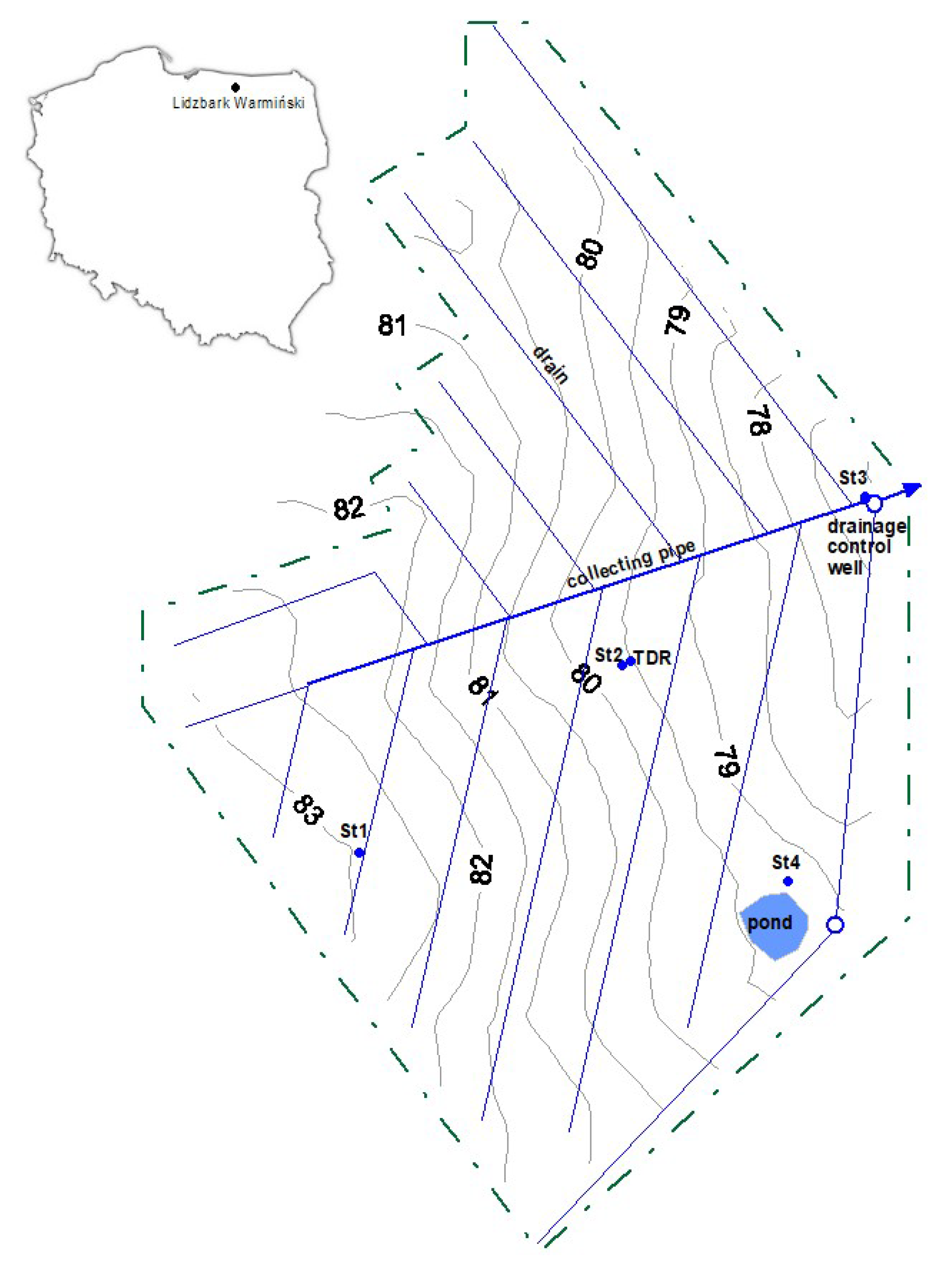
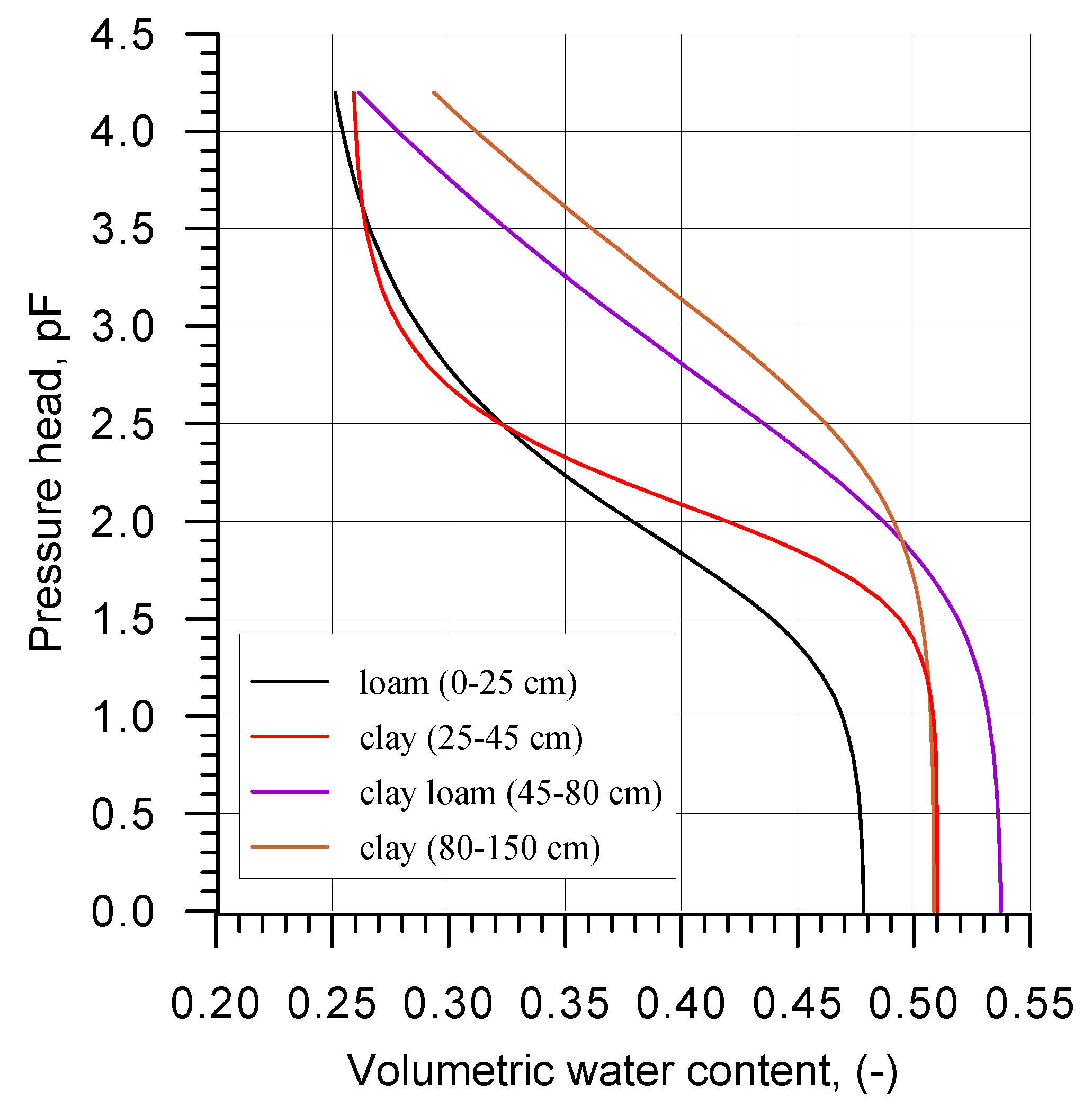
Field research was conducted at the Lidzbark Warmiński experimental site (54°08′ N, 20°35′ E), located in Warmińsko-Mazurskie province in Poland. Mollic Gleysols developed from loam and clay dominate in this area. According to USDA soil taxonomy [23], the representative soil profile is divided into four soil layers: loam (0–25 cm), clay (25–45 cm), clay loam (45–80 cm), and clay (80–150 cm). This soil is situated in hilly areas with slopes ranging between 2% and 4%. The winter wheat (Triticum L.) was cultivated in the 2011/12 seasons; the rape (Brassica napus) crop was cultivated in the 2012/13 season; and the winter barley (Hordeum L.) crop was cultivated in the 2013/14 season. The average yearly sum of precipitation for this region is 624 mm. The highest rainfall is usually observed in July and August. The vegetation period lasts about 200 days. A tile drainage system, with 21 m drain spacing and an average 0.9 m drain depth, occupies the experimental field. This drainage system is assembled with one collecting pipe (177 m long, with a 7.5 cm diameter) and thirteen drains (5 cm in diameter, with a total length of 1218 m) (Figure 1). The collecting pipe slopes up to 4%, and its catchment area equals 2.35 ha [24]. The drainage outflow was measured using an ultrasonic flow meter installed in a drainage control well. An ISCO 2150 ultrasonic flow meter (TELEDYNE ISCO, Lincoln, NE, USA) was used for testing, which had previously been adapted to measure the volume of drainage flows [25,26,27].
The flow meter was placed in a drainage control well, where an area velocity sensor (AV) was installed in a specially adapted outlet of the collecting pipe. To measure groundwater levels, Mini-Diver microprocessor recorders were installed in four measuring wells (St1–St4) to measure water level and temperature changes (Figure 1). Each recorder was programmed to record the groundwater level every 60 min. The groundwater level measured in St2 was taken for this research. Dielectric constant measurement for soil moisture calculation was carried out using the FOM/mts Easy Test device, whose operation is based on the TDR (time domain reflectometry) method. TDR probes were installed in four characteristic layers of a representative soil profile at the following depths: 15, 30, 50, and 80 cm. The location of the measuring point (TDR and St2; Figure 1) was chosen as representative for the entire drainage section. This point is located centrally in the studied area, in the middle of the slope and approximately in the middle of the drain spacing. A measurement of TDR was taken every two to three days during the growing season and about once a week outside the growing season. Meteorological measurements included precipitation, atmospheric pressure, temperature, and relative humidity. Rainfall measurements were taken using a Davis rain gauge with a logger and Odyssey software. This device enables the continuous measurement and recording of precipitation. Reference evapotranspiration (ET0) was calculated according to the Penman–Monteith formula recommended by the Food and Agriculture Organization [28,29]:
where:
- ET0—reference precipitation (mm);
- Δ—the slope of the vapor pressure curve (kPa °C−1);
- γ′—modified psychrometric constant (kPa °C−1);
- Rn′—the radiation factor (mm d−1);
- Ea—the aerodynamic factor (mm d−1).
To calculate the Penman–Monteith reference evapotranspiration, the following meteorological data are required: daily average air temperature, daily average relative humidity, average wind speed at the 2 m level, and solar radiation. Potential evapotranspiration was calculated by multiplying ET0 by the crop coefficient (kc), a coefficient expressing the difference in evapotranspiration between the cropped and reference grass surface. The crop coefficient expresses crop actual mass and development stage influence on the evapotranspiration value, in sufficient soil moisture content. It is dependent on crop type, development stage, and yield [29,30].
Soil water retention characteristics were elaborated based on previous research [31,32] and are presented in Figure 2.
Soil water retention curves were used to draw graphs of moisture distribution in the soil profile corresponding to the field capacity. The graphs presented in the next section are intended to present the dynamics of changes in soil moisture content relative to the level of the groundwater. These graphs were correlated with characteristic time intervals, determined on the basis of the rainfall–drainage outflow relationship.
Three characteristic case studies were considered in this paper:
- Case 1: Early spring (4–30 April 2012)—drain outflow caused by melting snow combined with heavy rainfall;
- Case 2: Spring (1–27 May 2013)—drain outflow caused by intensive rainfall over a few days;
- Case 3: Late autumn/early winter (1–27 December 2013)—drain outflow caused by precipitation over a long period.
Two values were introduced: the precipitation retention rate (prr) and the drainage outflow factor (df). The precipitation retention rate shows how much precipitation has been retained in soil during a given period (including retention used in the potential evapotranspiration process), and is calculated as in Equation (2).
where,
- P—precipitation (m3 ha−1);
- ETP—potential evapotranspiration (m3 ha−1);
- ΔSWR—soil water retention gradient (m3 ha−1);
The precipitation retention rate can be used to calculate the efficiency of precipitation use. A high value indicates more effective precipitation retention and use of water in the evapotranspiration process. The ideal value is 100%.
The drainage outflow factor is the ratio of drainage outflow to precipitation and other water inflows outside the area concerned (Equations (3) and (4)). Other factors (O) represent water balance components that could not be measured, such as surface runoff, interception, seepage, or surface and subsurface inflow. These values result from the soil-water balance.
where:
- Q—drainage outflow (m3 ha−1);
- O—other factors (m3 ha−1);
When O ≤ 0, the drainage outflow factor indicates a soil retention ability, while a high value indicates poor ability or soil moisture close to saturation. Interpretation is more difficult when O > 0, because it depends on whether it is in the context of an inflow from the outside or an outflow in the form of surface runoff. If there is an inflow from the outside, a high value of the df indicates that this water is being intercepted by the drainage system. If there is surface runoff, a high df value indicates a drainage system insufficiency.
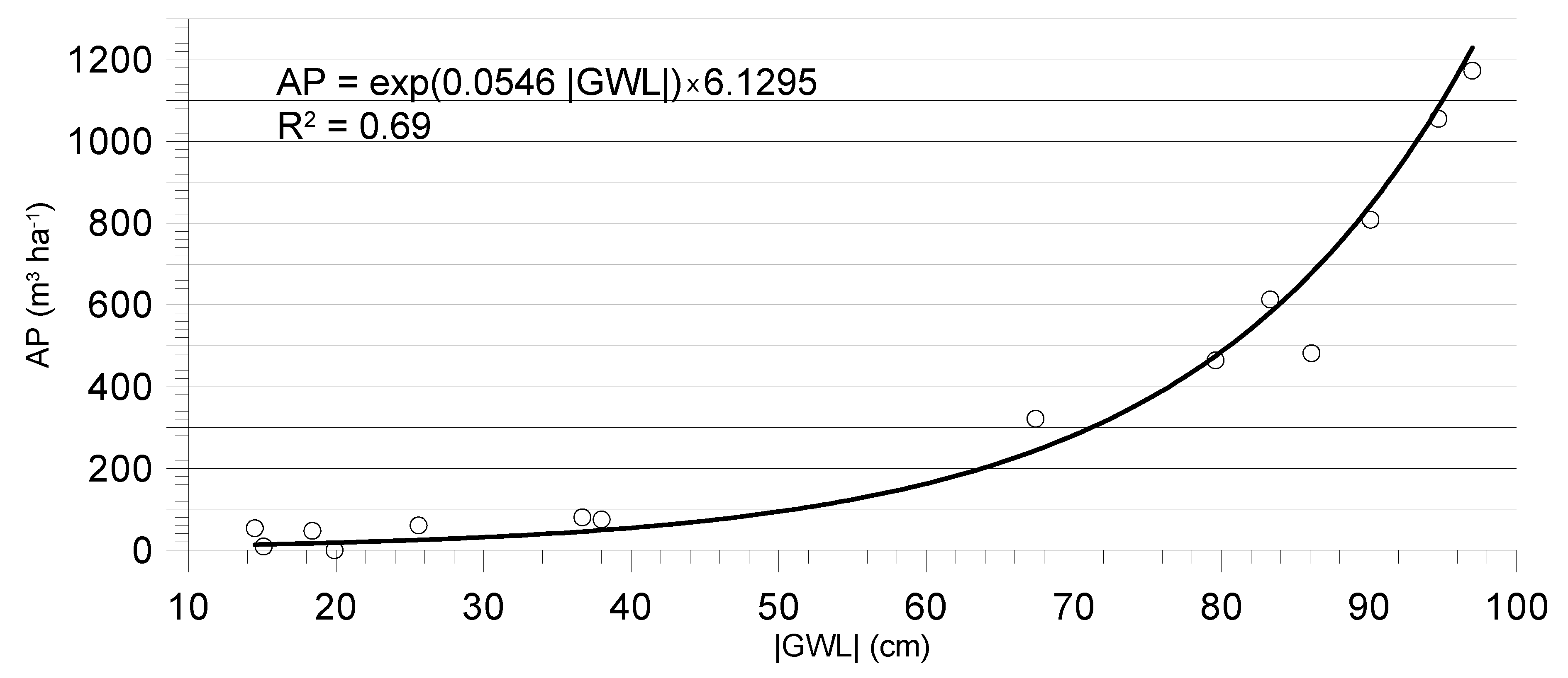
A relationship was also found between air porosity (AP) and the groundwater level (GWL), which is described by means of an exponential function:
where a and b are shape parameters.
This function applies to the range of the groundwater table (from 15 to 96 cm below ground level). With the help of the presented relationship (the known level of the groundwater table), it is possible to predict how much water from precipitation can potentially be retained in the soil.
3. Results and Discussion
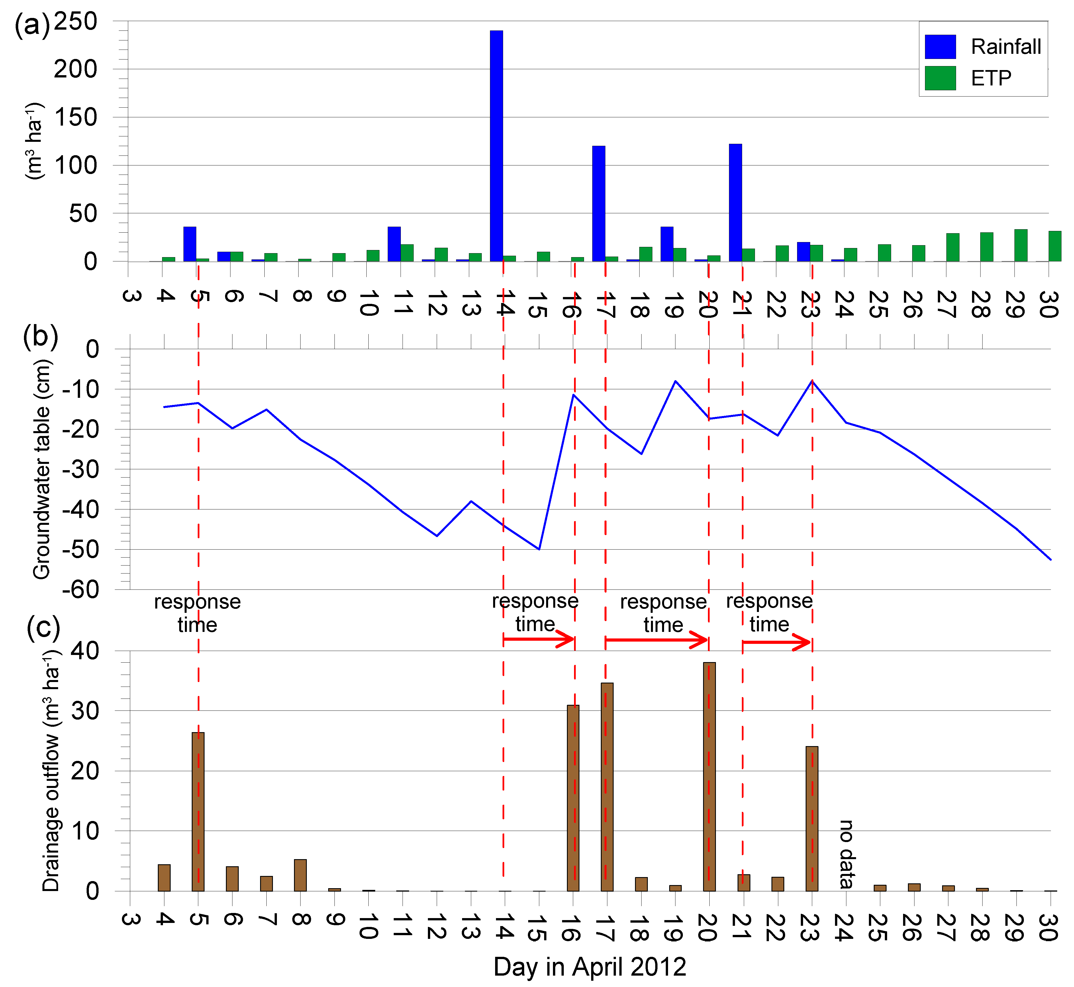
Figure 3 shows the relationships between precipitation, potential evapotranspiration, the groundwater table and drainage outflow for the considered cases.
Case 1: Early spring (4–30 April 2012)
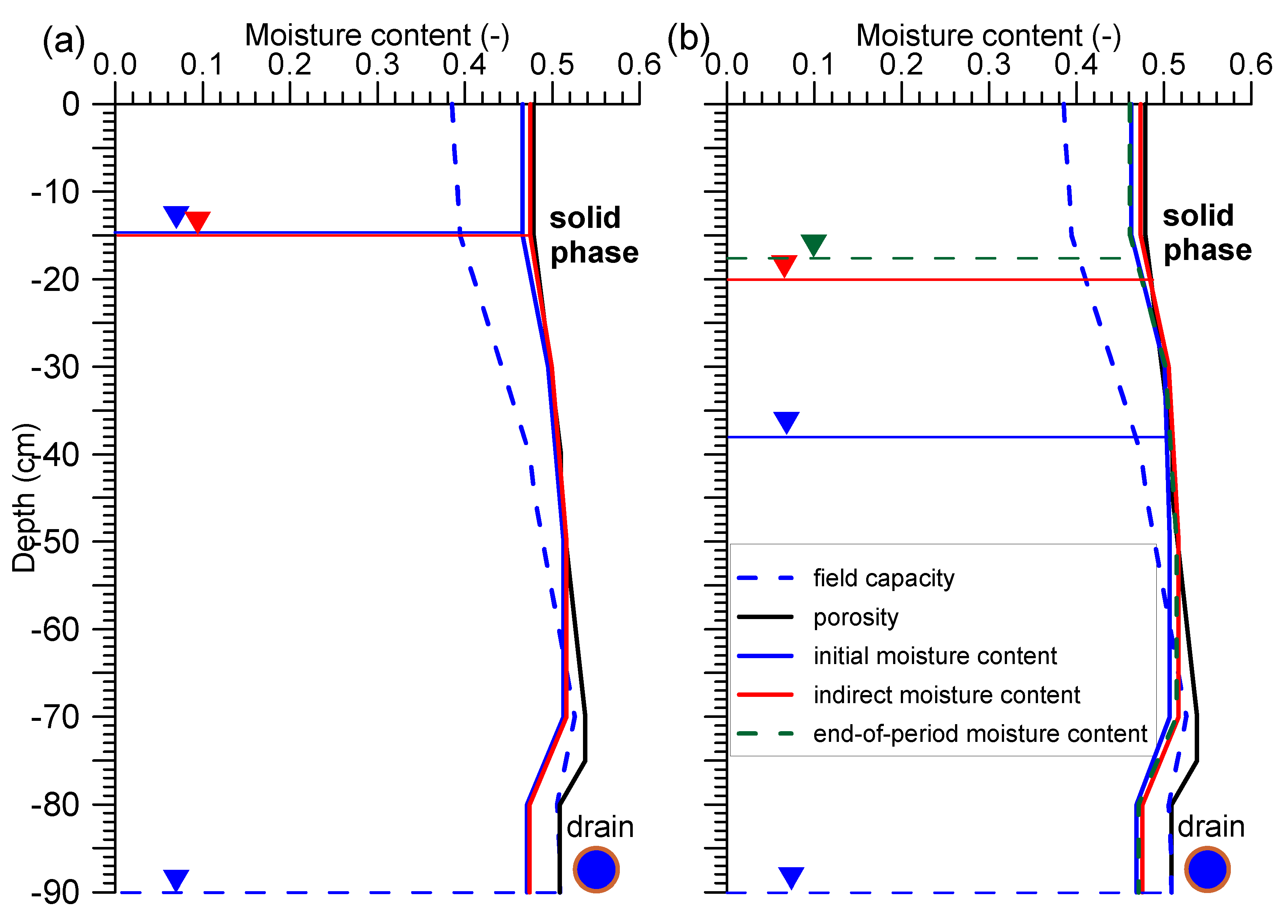
Field measurements started on 4 April. The groundwater level was 15 cm below the surface (Figure 3b), and soil moisture was close to the saturated water content (Figure 4a). There was a time of snow melting, so even light rainfall of 4 mm (40 m3 ha−1) caused an immediate reaction from the drainage system. Drainage outflow rose from a value of 4.4 to 26.4 m3 ha−1 (Figure 3c). Between 7 and 12 April, the groundwater level dropped steadily, reaching a value of −47 cm. On 14 April, there was very high rainfall (24 mm), as a result of which, after a day, the groundwater table began to rise significantly (up to −11 cm on 16 April). After two days, there was an intensive drainage outflow of 30.9 m3 ha−1. A significant rainfall of 12 mm (120 m3 ha−1) then took place on 17 April. The drainage system reacted for three days, during which the outflow value was 38.0 m3 ha−1. The last significant rainfall (12 mm) during the period in question occurred on 21 April. The response time of the water table and drain was two days. The groundwater level increased from −16 to −8 cm, and the drainage outflow from 2.3 to 24.1 m3 ha−1. A lack of rainfall after 24 April, ongoing drainage outflow, and an increase in potential evapotranspiration (to a value of about 3 mm d−1) contributed to a systematic lowering of the groundwater table towards the end of the study period. In order to consider the time taken for the groundwater table and drainage outflow to respond to precipitation, changes in the moisture content of the soil profile should be monitored at the same time. An example of changes in soil moisture content during the periods of 4–7 and 13–17 April are presented in Figure 4. Field capacity was determined from the pF curves, assuming the position of the groundwater table at drain level, when the soil solution was in equilibrium with the groundwater table. Initial moisture content should be understood as moisture on the first day of the period being studied, indirect moisture content as moisture on a specific day within the considered period; and final moisture content as the moisture on the last day of the considered period. Initial moisture content was close to the saturated water content, and the indirect moisture content was comparable with the saturated water content (Figure 4a), where the soil water table was kept at about −15 cm.
Starting from a depth of −55 cm, there was a discrepancy between soil porosity and saturated moisture content. In the −80 to −90 cm layer, this was about 2%. This discrepancy is probably a result of the measurement accuracy of the dielectric constant (±2%) [33] and the accuracy of the calculation based on it [34].
It is obvious that in such soil moisture conditions, even with light rainfall, the drainage outflow will increase immediately. After rainfall, the soil moisture level on 7 April was comparable to the saturated moisture content, with the groundwater table remaining at −15 cm.
Despite the fact that the groundwater table had dropped to −38 cm by 13 April, soil moisture in the top layer was only about 1% lower than porosity (Figure 4b). After the occurrence of high precipitation, the water table rose to −20 cm, and the soil moisture again reached a value comparable to the saturated water content. During the period under consideration, rainfall occurred several times (including two occasions with more than 10 mm d−1 rainfall), so the groundwater remained at a high level, and soil moisture was close to the saturated water content.
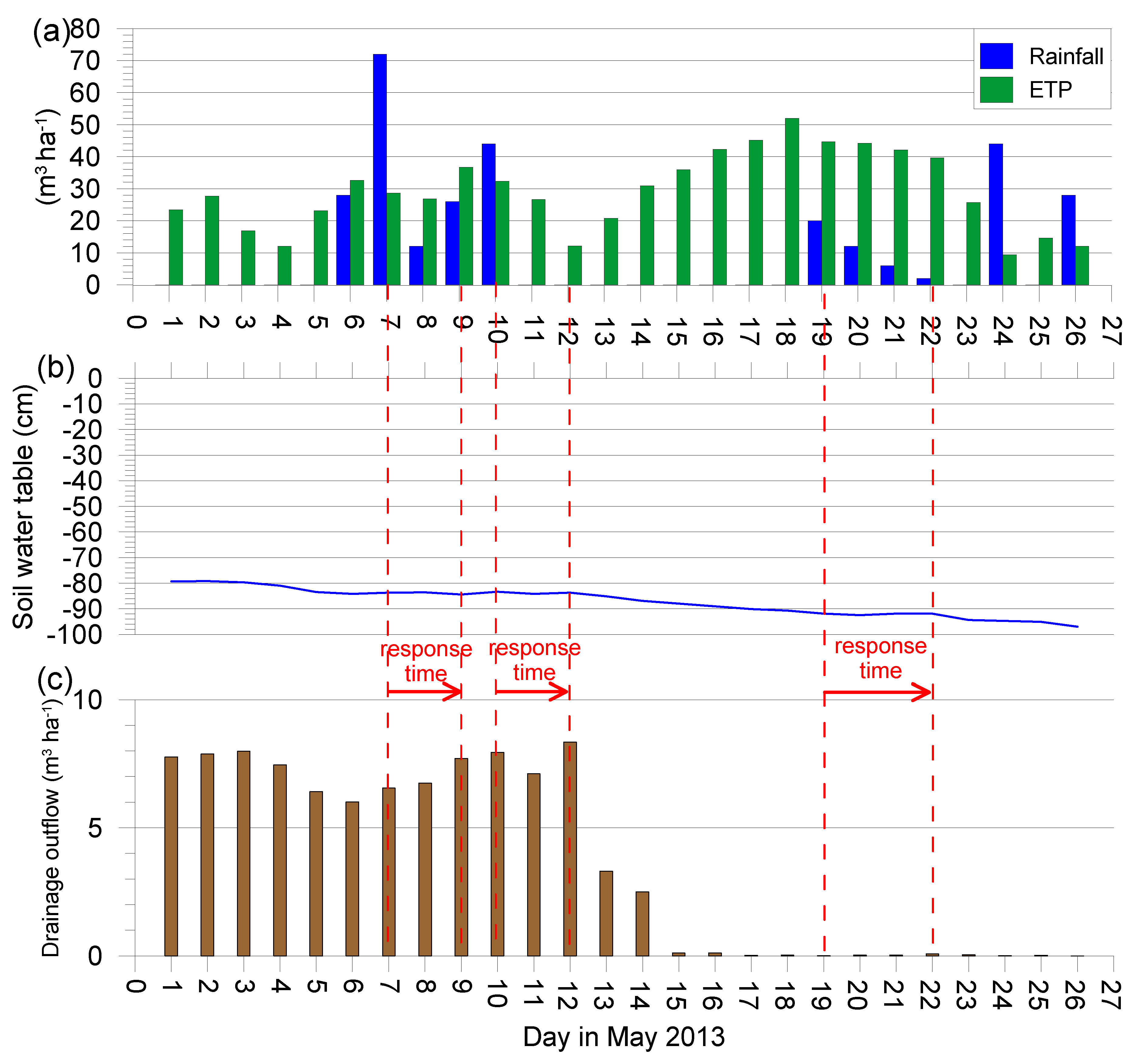
Case 2: Spring (1–27 May 2013)
Figure 5 shows the relationship between precipitation, potential evapotranspiration, the groundwater table and drainage outflow for considered period.
The beginning of May is a time of intensive plant growth, which systematically increases evapotranspiration (about 2.5 mm d−1 in the first ten days of May). Increasing evapotranspiration, a lack of rainfall during the preceding period, and drainage of excess water during early spring caused a systematic lowering of the groundwater table (Figure 5).
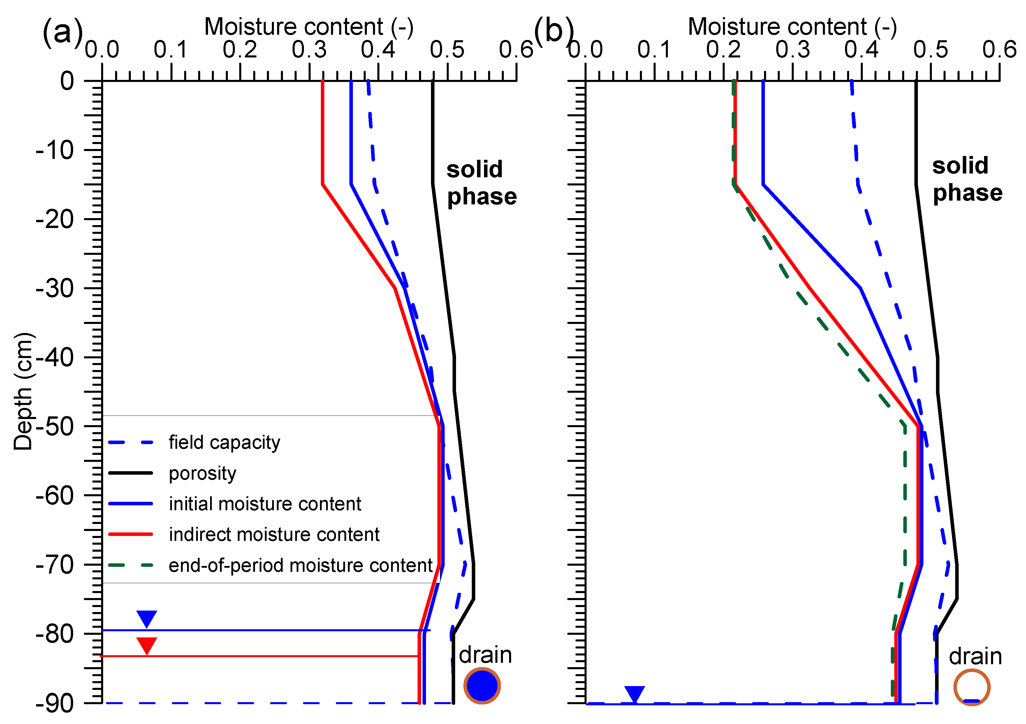
On 6 and 7 May, there was rainfall of 3 and 7 mm, respectively, which stopped the groundwater table from dropping further than −84 cm. Rain on the following two days did not cause the groundwater table to rise, but caused a slight increase in the drainage outflow (from 6.6 to 7.7 m3 ha−1). This was due to preferential flow through the resulting cracks, bypassing the soil matrix. Despite the preferential flow, the response time of the drainage system to precipitation was two days. Soil moisture also decreased during the first ten days of May (Figure 6a). At the end of this period, its retention capacity therefore increased by approximately 150 m3 ha−1 compared to the beginning of the month. Between 11 and 18 May, no rainfall was recorded, but evapotranspiration increased steadily (3.3 mm d−1 on average). From here, the groundwater table also gradually fell to a level below the drains. At this point, the drainage outflow finished.
Then, from 19 May, a four-day period began with low levels of rainfall (40 m3 ha−1 in total). The groundwater table remained around the drain level, and on the last rainy day, there was a very small drainage outflow (0.1 m3 ha−1). It can be assumed that the response time between precipitation and outflow was four days. Soil moisture continued to steadily decrease, and the soil water retention capacity therefore increased (Figure 6b). At the end of May, these increased by another 560 m3 ha−1, compared to the end of the first ten days.
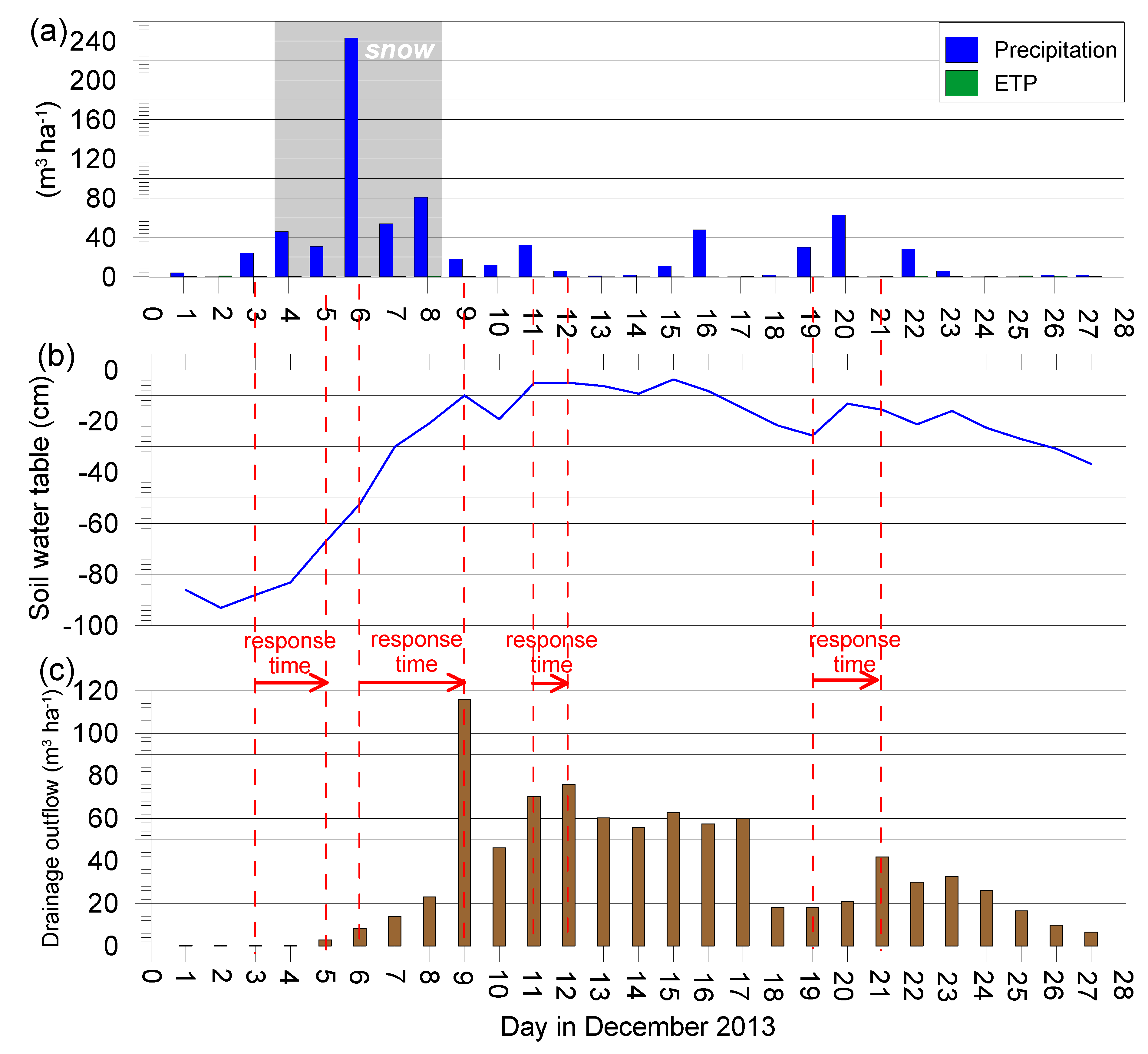
Case 3: Late autumn/early winter (1–27 December 2013)
Figure 7 shows the relationship between precipitation, potential evapotranspiration, the groundwater table and drainage outflow for considered period.
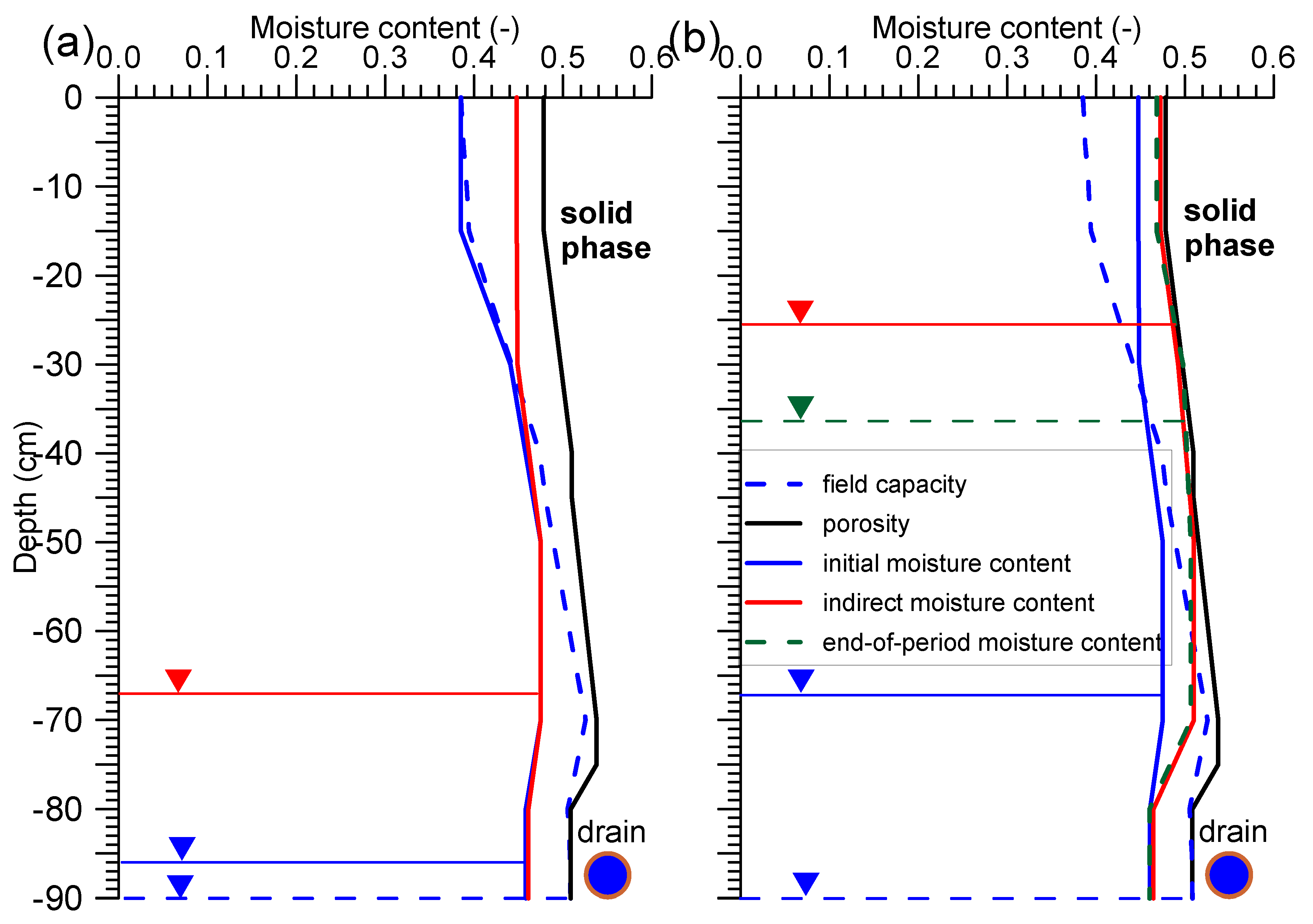
During the period under consideration, evapotranspiration no longer played a role because its average daily value was 0.4 m3 ha−1 (Figure 7a). It can be assumed that at the beginning of the first ten days of December, the volume of soil moisture corresponded to the field capacity (Figure 7b), with the groundwater table at −86 cm (Figure 7b). The precipitation period began on 3 December and lasted continuously for nine days. It should be noted that there was heavy snowfall between 4 and 8 December (Figure 7a). Calculated for the height of the water column, the total snowfall was 45.6 mm. The level of groundwater began to rise from the first day of precipitation, while a visible increase in drainage outflow occurred after two days (Figure 7c). Soil moisture increased significantly between 1 and 5 December (Figure 8a).
At this point, the soil was holding 160 m3 ha−1 of water. The most intense snowfall took place on 6 December, when 243 m3 ha of water fell during the day. Melting snow and further precipitation during the days that followed caused a rapid increase in drainage outflow, which amounted to 116.1 m3 ha on 9 December. The slight precipitation (3.2 m3 ha) that occurred on 11 December resulted in a visible reaction in the drainage outflow after one day. On that day, the groundwater level reached −10 cm. An average drainage outflow of 63.2 m3 ha−1 was maintained on the following six days. On 16 December, further precipitation measuring nearly 5 mm occurred but did not cause a clear increase in drainage outflow. The next rainfall of 3 mm (19 December) caused an increase in outflow from 18.1 to 41.9 m3 ha after two days. The soil reached a state of near saturation (Figure 8b—indirect moisture content). On 23 December, the groundwater table was at a level of −16 cm, and from that day onwards, began to drop systematically, reaching a value of −37 cm by the end of the period. Drainage outflow also decreased to 6.5 m3 ha−1 at the end of the period, and there was a slight decrease in soil moisture (although this was still close to full saturation).
At this point, an analysis will be presented of individual elements of the soil-water balance and soil water retention (rainfall, potential evapotranspiration, and drainage outflow relationship), with a summary of all three previously described cases (Table 1). Other factors are understood as the other components of the soil-water balance that were not measured due to technical limitations. Their values result from the water balance. Considering the location of the experimental site in the landform, it was assumed that a positive value indicated the inflow of water from the higher area. In contrast, a negative value indicated both surface runoff and/or deep percolation as well as interception. The theoretical level of water storage (saturated water content) in a soil profile 0.9 m deep, calculated according to the total porosity, was equal to 4551 m3 ha−1. From an experimental point of view, it can be assumed that saturated water content occurred on 7 and 17 April 2012 (Figure 4). The groundwater table was then at −15 and −20 cm, respectively. The soil water storage was then 4471 m3 ha−1 (rounded).
In both early spring and spring, the precipitation retention rate value was rounded to 34%. In the first case, significant surface runoff was observed during the site visit on 4 April. It was a consequence of melting snow and continuous rainfall from 27 March to 3 April 2012. The soil was close to full saturation, so the surface water could not infiltrate and outflow through the drainage system. In the second case, water loss was influenced by interception and seepage. Drainage outflow factor values were also very similar and oscillated around 29%. The plant cover was undergoing intensive growth. From 11 to 18 May 2013 there was no rainfall and the water level was steadily falling, so the negative O value can be explained by infiltration below the soil profile. In addition, some of the precipitation that occurred at the end of the considered period remained on the plant canopy and evaporated in the process of interception. In the third case, the precipitation retention rate was about 2% lower compared to cases 1 and 2. In contrast, the drainage outflow factor was more than twice as high and amounted to 68%. Heavy snowfall (especially on 6 December) played a very important role here, as its intensive melting during days when the air temperature rose above 0 °C caused an inflow of surface and subsurface water. Note that at the beginning of the considered period, soil moisture was less than field capacity (Figure 8). The soil retained 401 m3 ha−1, but drained away 875 m3 ha−1 anyway. This can be explained by the fact that water from melting snow came from the higher areas both in the form of surface runoff and underground inflow.
Finally, Figure 9 presents a graph of the relationship between groundwater level (GWL) and air porosity (AP). In order to develop the function, data on soil water retention in the soil profile for selected days in the considered time periods and the corresponding level of the groundwater table were used.
4. Conclusions
In the first phase of the early spring period, when rainfall caused intense melting of snow, the groundwater table was over a dozen centimeters below the surface, and the soil moisture was close to the saturated water content. Thus, even light rainfall caused an immediate reaction from the drainage system. Around mid-April, when the groundwater table dropped to half a meter, the drainage system reacted to precipitation after two to three days. In the early spring period, groundwater generally remained at a high level, and soil moisture was close to the saturated water content.
In the spring period, increasing evapotranspiration, lack of rainfall, and the drainage of excess water from the early spring period caused a systematic lowering of the groundwater table and the appearance of cracks. After precipitation, despite the occurrence of preferential flow, the drainage system worked after three days. At the same time, soil moisture continued to steadily decrease, and thus the soil water retention capacity increased.
In late autumn, soil moisture corresponded to field capacity, and evapotranspiration no longer played a role. Heavy snow and then rain caused the groundwater table to rise by about 80 cm and soil saturation within six days. At this point, the soil was holding 160 m3 ha−1 of stored water. The drainage system reacted two days after the first rainfall, and the largest outflow occurred after six days.
In both the early spring and spring periods, the precipitation retention rate value was rounded to 34%. Drainage outflow factor values were also very similar and oscillated around 29%. For the late autumn period, the precipitation retention rate value was about 2% lower than in the early spring and spring periods. In contrast, the drainage outflow factor was more than twice as high and amounted to 68%.
The greatest risk of flooding on agricultural land is snow melting rapidly under the influence of rain. Soil near a state of full saturation is not able to retain water, which means that intensive drainage outflow and surface runoff occurs during the day. In this case, it was found that the soil drainage system could not take over and delay the outflow, thus reducing the risk of flooding.
Funding
This research was funded by the Polish Ministry of Science and Higher Education, grant numbers. N N305 039234 and N N305 171840.
Acknowledgments
Special thanks to: Jan Szatyłowicz, Tomasz Gnatowski, Robert Michałowski and Ireneusz Cymes, for theirs invaluable help in conducting field work.
Conflicts of Interest
The author declare no conflict of interest.
References
- Groisman, P.Y. Trends in intense precipitation in the climate record. J. Clim. 2005, 18, 1326–1350. [Google Scholar] [CrossRef]
- Kundzewicz, Z.W.; Kowalczyk, P. Zmiany klimatu i ich skutki; Wydawnictwo KURPISZ S.A.: Poznań, Poland, 2008; p. 214. ISBN 978-83-75249-69-9. [Google Scholar]
- Kundzewicz, Z.W.; Pińskwar, I.; Brakenridge, R.G. Large floods in Europe, 1985–2009. Hydrol. Sci. J. 2013, 58, 1–7. [Google Scholar] [CrossRef]
- Ciepielowski, A. Charakterystyka zjawisk powodziowych w Polsce. In Ochrona przed powodzią; Ciepielowski, A., Mosiej, J., Eds.; Instytut Melioracji i Użytków Zielonych: Falenty, Poland, 1992; pp. 15–21. [Google Scholar]
- Romanowicz, R.J.; Nachlik, E.; Januchta-Szostak, A.; Starkel, L.; Kundzewicz, Z.W.; Byczkowski, A.; Kowalczak, P.; Żelaziński, J.; Radczuk, L.; Kowalik, P.; et al. Zagrożenia związane z nadmiarem wody. Nauka 2014, 1, 123–148. [Google Scholar]
- Kiciński, T. Ochrona przed powodzią; Wydawnictwo SGGW-AR: Warszawa, Poland, 1983; pp. 7–11. ISBN 83-00-01824-7. [Google Scholar]
- Jarosz, D. Historia powodzi w Polsce 1945–1989: Prolegomena do badań, Polska 1944/45–1989. Studia i Materiały XII/2014. Available online: https://rcin.org.pl/dlibra (accessed on 22 April 2020).
- Kledyński, Z. Flood control and infrastructure in Poland. Awarie budowlane. In Proceedings of the 2011, XXV Konferencja Naukowo-Techniczna, Międzyzdroje, Poland, 24–27 May 2011. [Google Scholar]
- Kowalewski, Z. Powodzie w Polsce—Rodzaje, występowanie oraz system ochrony przed ich skutkami. Water-Environ. Rural Areas 2006, 6, 207–220. [Google Scholar]
- Mioduszewski, W. Zjawiska ekstremalne w przyrodzie—Susze i powodzie. In Wybrane Problemy Ochrony Mokradeł; Łachacz, A., Ed.; Uniwersytet Warmińsko-Mazurski w Olsztynie: Olsztyn, Poland, 2012; pp. 57–74. [Google Scholar]
- Grzywna, A. Quantity of water retention in the reclaimed valley mid-forest (Forest Parczew). Sci. Rev. Eng. Environ. Sci. 2014, 64, 124–130. [Google Scholar]
- Liberacki, L.; Bykowski, J.; Kozaczyk, P.; Skwierawski, M. Ocena konserwacji i modernizacji urządzeń melioracji podstawowych na obszarze Północnej Wielkopolski. Ecol. Eng. 2016, 49, 66–73. [Google Scholar]
- Skaggs, R.W.; Schilfgaarde, J. Introduction. In Agricultural Drainage No. 38 Agronomy; Skaggs, R.W., Schilfgaarde, J., Eds.; ASA, CSSA, SSSA Publishers: Madison, WI, USA, 1999; pp. 3–10. [Google Scholar]
- Kladivko, E.J.; Grochulska, J.; Turco, R.F.; Van Scoyoc, G.E.; Eigel, J.D. Pesticide and Nitrate Transport into Subsurface Tile Drains of Different Spacings. J. Environ. Qual. 1999, 28, 997–1004. [Google Scholar] [CrossRef]
- Kladivko, E.J.; Frankenberger, J.R.; Jaynes, D.B.; Meek, D.W.; Jenkinson, B.J.; Fausey, N.R. Nitrate Leaching to Subsurface Drains as Affected by Drain Spacing and Changes in Crop Production System. J. Environ. Qual. 2004, 33, 1803–1813. [Google Scholar] [CrossRef] [PubMed]
- Kladivko, E.J.; Willoughby, G.L.; Santini, J.B. Corn Growth and Yield Response to Subsurface Drain Spacing on Clermont Silt Loam Soil. Agron. J. 2005, 97, 1419–1428. [Google Scholar] [CrossRef]
- De Schepper, G.; Therrien, R.; Refsgaard, J.C.; Lausten Hansen, A. Simulating coupled surface and subsurface water flow in a tile-drained agricultural catchment. J. Hydrol. 2015, 521, 374–388. [Google Scholar] [CrossRef]
- Spoor, G.; Leeds-Harrison, P.B. Nature of Heavy Soils and Potential Drainage Problems. In Agricultural Drainage No. 38 Agronomy; Skaggs, R.W., Schilfgaarde, J., Eds.; ASA, CSSA, SSSA Publishers: Madison, WI, USA, 1999; pp. 1051–1081. [Google Scholar]
- Robinson, M.; Rycroft, D.W. The Impact of Drainage on Streamflow. In Agricultural Drainage No. 38 Agronomy; Skaggs, R.W., Schilfgaarde, J., Eds.; ASA, CSSA, SSSA Publishers: Madison, WI, USA, 1999; pp. 767–800. [Google Scholar]
- Irwin, R.W.; Hugh, R.; Whiteley, H.R. Effects of Land Drainage on Stream Flow. Can. Water Resour. J. 1983, 8, 88–103. [Google Scholar] [CrossRef]
- Dembek, W. Melioracje wodne a współczesna ochrona przyrody. In Kontrola Państwowa Numer 1 Specjalny; Repetowska-Nyc, M., Kulicka, J., Odolińska, B., Eds.; Najwyższa Izba Kontroli: Warszawa, Poland, 2011; pp. 34–47. [Google Scholar]
- Pierzgalski, E. Systemy i urządzenia melioracyjne. In Kontrola Państwowa Numer 1 Specjalny; Repetowska-Nyc, M., Kulicka, J., Odolińska, B., Eds.; Najwyższa Izba Kontroli: Warszawa, Poland, 2011; pp. 48–60. [Google Scholar]
- SSSA. Glossary of Soil Science Terms; SSSA: Madison, WI, USA, 1997; pp. 101–102. [Google Scholar]
- Szejba, D.; Papierowska, E.; Cymes, I.; Bańkowska, A. Nitrate nitrogen and phosphate concentrations in drainflow: An example of clay soil. J. Elem. 2016, 21, 899–913. [Google Scholar] [CrossRef]
- Szejba, D.; Bajkowski, S.; Pietraszek, Z. The capabilities of ultrasonic meters utilization for flow measurements in drainage pipelines. In Hydrology in Engineering and Water Management T. 1; Więzik, B., Ed.; Committee of Environmental Engineering Monograph Polish Academy of Science: Warszawa, Poland, 2010; Volume 68, pp. 439–449. [Google Scholar]
- Szejba, D.; Bajkowski, S.; Pietraszek, Z. The outflow measurement under the conditions of drainage pipe submergence. Adv. Agric. Sci. Probl. Issues 2011, 564, 263–271. [Google Scholar]
- Szejba, D.; Bajkowski, S. Determination of Tile Drain Discharge Under Variable Hydraulic Conditions. Water 2019, 11, 120. [Google Scholar] [CrossRef] [Green Version]
- Allen, R.G.; Pereira, L.S.; Raes, D.; Smith, M. Crop Evapotranspiration (Guidelines for Computing Crop Water Requirements); FAO Irrigation and Drainage Paper No. 56: Rome, Italy, 2000; pp. 17–28. [Google Scholar]
- Szejba, D. Evapotranspiration of Grasslands and Pastures in North-Eastern Part of Poland. In Evapotranspiration–Remote Sensing and Modeling; Irmak, A., Ed.; InTech: Rijeka, Croatia, 2012; pp. 179–196. [Google Scholar]
- Łabędzki, L.; Szajda, J.; Szuniewicz, J. Ewapotranspiracja upraw rolniczych—Terminologia, definicje, metody obliczania. In Materiały informacyjne IMUZ; Wydawnictwo IMUZ: Falenty, Poland, 1996; pp. 1–7. [Google Scholar]
- Szejba, D.; Cymes, I.; Szatyłowicz, J.; Szymczyk, S. An impact of drainage system on soil water conditions at Lidzbark Warmiński experimental site. Biologia 2009, 64, 565–569. [Google Scholar] [CrossRef]
- Szejba, D.; Szatylowicz, J.; Jaczewska, M. Zastosowanie urządzenia EQUI-pF do określenia parametrów retencyjnych i hydraulicznych gleby ciężkiej metodą zadania odwrotnego. Acta Scientiarum Polonorum Formatio Circumiectus 2013, 2, 12. [Google Scholar]
- Institute of Agrophysics Polish Academy of Sciences. MANUAL FOM/mts and TDR/MUX/mpts and TDR/MUX/mpts/dlog Ver. 1.41; Institute of Agrophysics Polish Academy of Sciences: Lublin, Poland, 2013; pp. 31–38. [Google Scholar]
- Malicki, M.A.; Plagge, R.; Roth, C.H. Improving the calibration of dielectric TDR soil moisture determination taking into account the solid soil. Eur. J. Soil Sci. 1996, 47, 357–366. [Google Scholar] [CrossRef]
Figure 1.
Visual location and scheme of the experimental site.

Figure 2.
Soil moisture retention curves for individual soil layers.

Figure 3.
Daily precipitation and potential evapotranspiration (ETP) values (a), groundwater table (b), and drainage outflow (c) during the April 2012 observation period.
Figure 3.
Daily precipitation and potential evapotranspiration (ETP) values (a), groundwater table (b), and drainage outflow (c) during the April 2012 observation period.

Figure 4.
Changes in soil moisture content during the periods 4–7 April (a) and 13–24 April (b).

Figure 5.
Daily values of precipitation and potential evapotranspiration (a), groundwater table (b), and drainage outflow (c) during the May 2013 observation period.
Figure 5.
Daily values of precipitation and potential evapotranspiration (a), groundwater table (b), and drainage outflow (c) during the May 2013 observation period.

Figure 6.
Changes in soil moisture content during the periods 3–10 May (a) and 17–27 May (b).

Figure 7.
Daily values of precipitation and potential evapotranspiration (a), groundwater table (b), and drainage outflow (c) during the December 2013 observation period.
Figure 7.
Daily values of precipitation and potential evapotranspiration (a), groundwater table (b), and drainage outflow (c) during the December 2013 observation period.

Figure 8.
Changes in soil moisture content during the periods 1–5 December (a) and 5–27 December (b).
Figure 8.
Changes in soil moisture content during the periods 1–5 December (a) and 5–27 December (b).

Figure 9.
Relationship between groundwater level (GWL) and air porosity (AP).


Table 1.
Elements of the water balance in the drainage system catchment scale during the periods under consideration.
Table 1.
Elements of the water balance in the drainage system catchment scale during the periods under consideration.
| Period | SWRini | P | ETP | Q | SWRend | ΔSWR | O | prr | df | |
|---|---|---|---|---|---|---|---|---|---|---|
| Value | Remarks | |||||||||
| 4–24 April 2012 | 4417 | 632 | 207 | 179 | 4423 | 6 | −240 | surface runoff | 33.7 | 28.3 |
| 3–24 May 2013 | 4006 | 266 | 681 | 79 | 3415 | −591 | −98 | interception deep percolation | 33.7 | 29.5 |
| 1–27 December 2013 | 3989 | 746 | 10 | 875 | 4390 | 401 | 540 | outside subsurface and surface water inflow | 32.0 | 68.0 |
Where, SWRini—initial soil water retention (m3 ha−1); P—precipitation (m3 ha−1); ETP—potential evapotranspiration (m3 ha−1); Q—drainage outflow (m3 ha−1); SRWend—final soil water retention (m3 ha−1); ΔSWR—soil water retention gradient (m3 ha−1); O—other factors (m3 ha−1); prr—precipitation retention rate (%); df—drainage outflow factor (%).
© 2020 by the author. Licensee MDPI, Basel, Switzerland. This article is an open access article distributed under the terms and conditions of the Creative Commons Attribution (CC BY) license (http://creativecommons.org/licenses/by/4.0/).
Share and Cite
MDPI and ACS Style
Szejba, D. Importance of the Influence of Drained Clay Soil Retention Properties on Flood Risk Reduction. Water 2020, 12, 1315. https://doi.org/10.3390/w12051315
AMA Style
Szejba D. Importance of the Influence of Drained Clay Soil Retention Properties on Flood Risk Reduction. Water. 2020; 12(5):1315. https://doi.org/10.3390/w12051315
Chicago/Turabian StyleSzejba, Daniel. 2020. "Importance of the Influence of Drained Clay Soil Retention Properties on Flood Risk Reduction" Water 12, no. 5: 1315. https://doi.org/10.3390/w12051315
Note that from the first issue of 2016, this journal uses article numbers instead of page numbers. See further details here.