Condition for the Incipient Motion of Non-Cohesive Particles Due to Laminar Flows of Power-Law Fluids in Closed Conduits

Abstract

The results of an experimental study on the condition of incipient transport of non-cohesive particles due to the flow of a power-law fluid in a rectangular pipe are presented in this article. The pipe can change its inclination, and experiments were carried out with positive and negative slopes. From a dimensional analysis, the parameters that define the condition of incipient motion were found and validated with experimental data. Thus, the threshold condition is well defined by a particle Reynolds number and a Galileo number, properly modified to take into account the power-law rheology of the fluid. The experimental data are also presented in a standard Shields diagram, including the data obtained in other studies carried out in open-channel laminar flows of Newtonian and power-law fluids.

1. Introduction and Objective

The flow of non-Newtonian fluids over non-cohesive granular beds can be found as much in industry as in nature [1,2,3]. The flow of slurry in pipes in the mining industry is usually transported with a mean flow velocity defined as the maximum between the critical velocity for turbulent flow and the critical velocity that precludes deposition of the solid particles [4]. However, under certain non-desirable operating conditions, the flow velocity can decrease, and larger particles of the slurry settle. The mixture formed by the finer, non-settling particles and the carrying fluid (water) behaves as an equivalent non-Newtonian fluid that can be modeled as power-law (or Ostwald–de Waele) fluid [5]. The deposit of the coarser particles forms a bed in the pipe, reducing its carrier capacity and increasing head losses [5]. Once the deposit is generated, it needs to be removed by the flow. In this context, the goal of this article is to present the results of an experimental study aiming to define the condition of incipient motion at which the particles start to move, due to the action of a laminar flow of a power law fluid. The fluid mimics the rheology of the mixture of water and fine sediments of the slurry.

The condition of incipient motion has been approached in two different ways: by determining a critical threshold velocity or in terms of a critical shear stress [6]. The analysis that follows is based in the second approach, which was first proposed by Shields in his doctoral thesis [7] that dealt with the incipient motion of granular, non-cohesive particles in open-channel turbulent flow. Shields related a dimensionless shear stress, ${\tau }_{*}={\tau }_0/\left(\left({\rho }_S-\rho \right)gd\right)$, with the particle Reynolds number, $R{e}_{*}=u_{*}d/\nu$, where ${\tau }_0$ is the bottom shear stress, $g$ is the acceleration due to gravity, $d$ is the sediment characteristic diameter, ν is the kinematic viscosity, ${\rho }_S$ and $\rho$ are the density of the sediment and fluid, respectively, and $u_{*}=\sqrt{{\tau }_0/\rho }$ is the frictional velocity. Shields presented graphically his experimental data, without fitting any curve to them. Rouse [8] added additional data and fitted a curve, resulting in the so-called Shields diagram as we know it today. Because of its importance in river mechanics, most of the research on the critical Shield stress has been developed for turbulent water flows in open channels [9,10]. The effect of the channel slope on the threshold of motion has been studied by several authors, and the relation between the critical shear stress in a channel inclined an angle $\theta$, ${\tau }_{\theta },$ with respect to the horizontal one, ${\tau }_{\theta =0}$, is given by ${\tau }_{\theta }/{\tau }_{\theta =0}=\cos \theta \left(1-\tan \theta /\tan \alpha \right)$, where $\alpha$ is the angle of repose of the sediment [10]. This relationship is independent of the flow regime. Studies involving a laminar regime are not as abundant as in turbulent flows. Among them, the research developed by the following authors can be mentioned: White [11], Mantz [12], Yalin and Karahan [13], and Pilotti and Menduni [14]. These studies present their results following the approach proposed by Shields, finding a relationship between ${\tau }_{*}$ and $R{e}_{*}$. Alternatively, other dimensionless parameters have been used. For example, Cheng [15] defines the incipient condition in terms of $R{e}_{*}$ and a dimensionless particle diameter defined as $d_{*}=d{\left(\left({\rho }_S-\rho \right)g/\left({\rho \nu }^2\right)\right)}^{1/3}$.

The condition of incipient motion in closed, pressurized conduits has also been presented in terms of the Shields diagram for flows in pipes in the transitional regime and low Reynolds turbulent flows [16]. For laminar flows in inclined Hele–Shaw cells (20 cm wide, 130 cm long, and a 2 mm gap), Loiseleux et al. [17] presented the critical Shields stress as a function of a particle Reynolds number based on the mean flow velocity $U$, $Re=Ud/\nu$. From experiments with laminar flows in horizontal cylindrical pipes (3 cm diameter and 180 cm long), Ouriemi et al. [18] concluded that, for small particle Reynlolds numbers, the critical shear stress takes a constant value. In their article, they define a dimensionless parameter (written as $R{e}_p/Ga$) that involves the usual Shields stress, sediment size, pipe diameter $D$, water depth $h_f$, and a numerical coefficient. For the incipient condition, Ouriemi et al. find that $\left(R{e}_p/Ga\right)~{\left(h_f/D\right)}^2$. Lobkovsky et al. [19] conducted experiments in a horizontal conduit with a rectangular cross-section (3.3 cm high, 2.6 cm wide, 40.5 cm long, with the sediment in the central 24.6 cm of the duct), obtaining that, for their experimental flow condition, the critical shear stress agrees with Shields’criteria. Rabinovich and Kalman [20], from experiments in a square duct (a wind tunnel with a 10 × 10 cm² section and 6 m long), found that the incipient motion condition can be expressed in terms of a particle Reynolds number based on the mean flow velocity adapted to consider the duct geometry, and a modified Archimedes number, defined as $A{r}^{*}=fAr$, where $f$ is the static friction coefficient between the particle and the bottom and $Ar=\rho \left({\rho }_S-\rho \right)g{d}^3/{\mu }^2$, with $\mu$ as the fluid dynamic viscosity. $Ar$ is also known as the Galileo (or Galilei) number, $Ga$. Hong et al. [21], from experiments in the facility used by Lobkovsky et al. [19], reported the critical condition in a Shields fashion graph. In their paper, both the Shields stress and particle Reynolds number are defined in terms of the shear rate. Other authors [22,23,24] have approached the problem as one of instability of a deformable bed, predicting the threshold condition in terms of the Shields stress, Galileo number, and $d/h_f$ [22,23]. Ouriemi et al. [24], present Charru and co-workers’ results as a relation between the pipe Reynolds number and $Ga{\left(h_f/d\right)}^2$.

Except for the work in open channels carried out by Tamburrino et al. [6], the rest of the references mentioned before deal with Newtonian fluids, mostly water. In spite of their importance in the industry, articles on incipient motion due to non-Newtonian fluid flows are rather scarce. As far as the authors are aware, the only studies with non-Newtonian fluids are those reported by Daido [25] and Wan [26] in which clay–water mixtures were modeled as Bingham plastic fluids, and the already mentioned work by Tamburrino et al., with power-law fluids. No reports of incipient motion due to shear thinning fluid flows in closed conduits were found by the authors in the available literature. It has to be noted that in slurry transport, the critical condition (usually given by a critical velocity) refers to the flow condition at which no particle settling occurs, which is different to the problem presented in this article, as stated in the first paragraph of the Introduction.

2. Experimental Setup and Materials

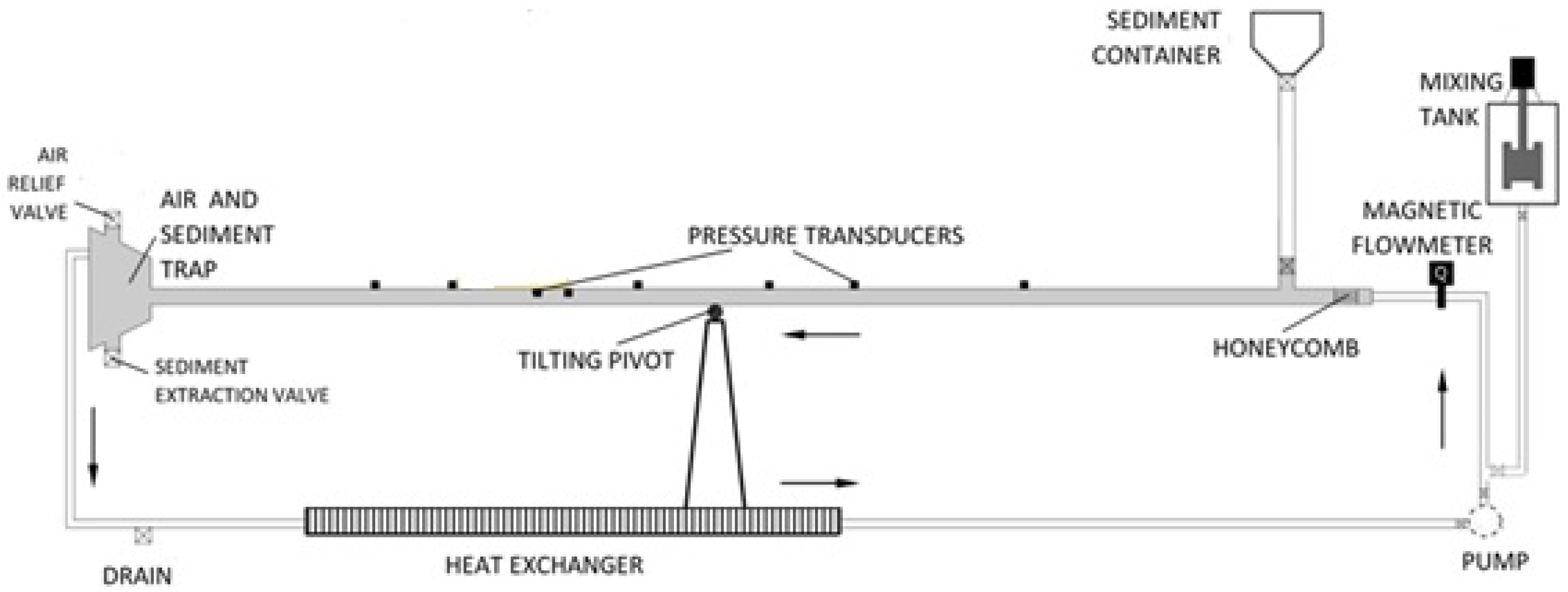
A sketch of the experimental setup is shown in Figure 1. It consists in a closed circuit where a square tilting pipe is located. The cross-section area is 52 × 52 mm², and the pipe is 10 m long. The inclination angle of the pipe with respect to a horizontal datum can change between −17.5 and 17.5°. The circuit is closed by means of two hoses that join the square pipe to a cylindrical one, connected to a stainless steel centrifugal pump. A heat exchanger installed in the system allows the control of temperature during the experiments. Air and sediment traps are located in the downstream end of the square pipe. Two reservoirs are located at the upstream end of the pipe. One of them contains the sediments used to generate the granular bed in the pipe, as described later. The second reservoir serves two purposes: (i) as a mixing tank to prepare the CMC aqueous solutions to be tested, and (ii) as a reservoir that contains the non-Newtonian mixtures that will fill the closed circuit before the experiment starts. A built-in mixer in the container permits achieving the first purpose. The square pipe was built using a transparent perspex, 10 mm thick. The discharge was measured with a magnetic flowmeter Siemens model SITRANS F M MAG 3100 (Siemens, Lille, France). Eight pressure transducers made by OMEGA model PX409-2.5DWUV (Measurements Specialties, Inc., Hampton, VA, USA) were installed along the pipe and connected to a data acquisition system. Particle motions were recorded by a camera NIKON D800 (Nikon, Tokyo, Japan) installed normal to the top wall, and by a camera GoPro Hero 3 (GoPro, San Mateo, CA, USA) placed normal to one of the vertical walls.

The sediments used in the experiments correspond to quartz sand, whose physical characteristics are presented in

Table 1. Sediment properties.

Sand	Size Range (mm)	$\mathit{d}$ (mm)	$\mathit{\alpha }$ (°)	${\mathit{\rho }}_{\mathit{S}}$ (kg/m3)
A	1.0–1.3	1.15	29	2700
B	0.4–0.6	0.50	31	2650
C	1.6–2.36	1.98	29	2700
D	2.36–3.35	2.86	29	2700

. In the table, $d$ is the nominal size, $\alpha$ is the angle of repose, and ${\rho }_S$ the sediment density.

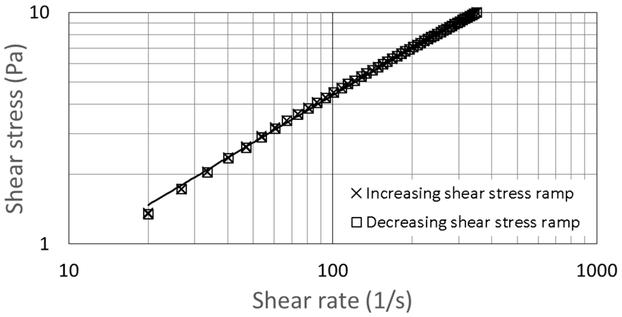
The shear thinning fluids were aqueous solutions of sodium carboxymethyl cellulose (CMC), and their rheology was determined with a rheometer Anton Paar model Rheolab QC (Anton Paar, Inc., Ashland, VA, USA) with concentric cylinders. The solutions behaved as power law fluids, with a constitutive equation given by ${\tau }_{ij}=K{\dot{\gamma }}^{n-1}{\dot{\gamma }}_{ij}$, where ${\tau }_{ij}$ is the shear stress tensor, ${\dot{\gamma }}_{ij}$ is the shear rate, and $\dot{\gamma }$ its second invariant. $K$ and $n$ are the consistency coefficient and the flow index, respectively. As an example, Figure 2 presents the rheogram corresponding to the water–CMC mixture used in Experiment 13 (described in Table S1 of the online supplementary material). The solutions used in the experiments had flow indexes in a range of 0.58–0.76 and consistency coefficient between 0.10 and 0.56 Pa × sⁿ. Density was practically equal to the water in which the CMC was mixed. The solutions resulting from the CMC–water mixture are transparent, allowing visualization of the bed particles.

All the mixtures were carefully blended in the mixing tank to avoid formation of solid lumps in the CMC solutions. Then, with the pipe inclined such that the air tramp was at the highest height, in order to allow the air to escape through the air relief valve, the circuit was filled with the water–CMC solution. Next, the pipe was positioned horizontally and the valve connecting the sediment container was opened and the sand incorporated to the circuit. A flow was generated with a velocity high enough to keep all the sediment particles in suspension for a while. Then, the flow was stopped, allowing the particles to settle and to generate a horizontal bed, with a thickness that depended on the test. Finally, before starting the experiment, the pipe was set at the desired inclination. The angle of inclination ranged from −9.89 to 10.38°, and the discharge was between 0.16 and 1.96 m³/h. Entrance length was estimated from the Kim et al. relationship [27], which indicates that for the experimental conditions tested, the length to have a fully developed flow was around 10 cm or less.

Following Tamburrino et al. [6], three modes of particle motion were defined: no motion, incipient, and generalized, and they were identified visually. In the central part of the pipe, an observation area was defined (roughly 5 cm wide and 10 cm long). When in the observation window a continuous motion of several independent particles was observed (about 1% of the surface particles), the transport mode was considered as incipient. As an example of this condition, a video (Video S1) is presented as supplementary material, corresponding to Experiment 1 of the Table S1. In the generalized motion, most of the particles were observed in a continuous motion (without reaching a sheet flow regime). Although the above criteria are subjective, they were shown to be robust, as noted in Section 4.

The flow regime for all the experiments was laminar, according to Dodge and Metzner’s criterion [28] using the pipe Reynolds number modified by Kozicki et al. [29] for power-law fluids in rectangular ducts. They defined ${Re}^{\prime }={\left(n/\left(a+bn\right)\right)}^n\rho U^{2-n}{R}_H^n/\left(2^{n-3}K\right)$, where $R_H$ is the hydraulic radius and $a$ and $b$ are parameters that depend on the aspect ratio of the section, presented in [29]. The flow is laminar for ${Re}^{\prime }<2100$ [28], and the experiments carried out in the study reported in this article were in the range of $5\le {Re}^{\prime }\le 305$. As the flow regime was laminar, no secondary currents were generated near the corners that could alter the incipient movement of the particles.

3. Dimensional analysis

Calling, as usual, the dimensions of force, length, and time as $\mathrm{F}$, $\mathrm{L}$, and $\mathrm{T}$, respectively, and denoting them in brackets, the variables (and dimensions) characterizing the fluid are its density $\rho$ $\left({\mathrm{FL}}^{-4}{\mathrm{T}}^2\right)$, consistency coefficient $K$ $\left({\mathrm{FL}}^{-2}{\mathrm{T}}^n\right)$, and flow index $n$ $\left({\mathrm{F}}^0{\mathrm{L}}^0{\mathrm{T}}^0=1\right)$. The sediment is characterized by its diameter $\left(\mathrm{L}\right)$, submerged specific weight $\left({\rho }_S-\rho \right)g$ $\left({\mathrm{FL}}^{-3}\right)$, and angle of repose $\alpha$ $\left({\mathrm{F}}^0{\mathrm{L}}^0{\mathrm{T}}^0=1\right)$. The motion of a particle is assumed to be the result of the critical shear stress acting on it, ${\tau }_c$ $\left({\mathrm{FL}}^{-2}\right)$, and the inclination of the bottom, given by the angle $\theta$ $\left({\mathrm{F}}^0{\mathrm{L}}^0{\mathrm{T}}^0=1\right)$. Thus, Buckingham’s Π theorem says that the problem is defined by five dimensionless parameters [30]. Choosing $\left(\rho , K,d\right)$ as the set of repeating variables, the following dimensionless parameters are found:

$${\Pi }_1=n$$

(1)

$${\Pi }_2=\theta$$

(2)

$${\Pi }_3=\alpha$$

(3)

$${\Pi }_4=\frac{\left({\rho }_S-\rho \right)g{\rho }^{n/\left(2-n\right)}{d}^{\left(2+n\right)/\left(2-n\right)}}{K^{2/\left(2-n\right)}}$$

(4)

$${\Pi }_5={\tau }_0{\left(\frac{{\rho }^n{d}^{2n}}{K^2}\right)}^{1/\left(2-n\right)}$$

(5)

The functional relationship among the different dimensionless parameters and the dimensionless shear stress is given by:

$${\tau }_0{\left(\frac{{\rho }^n{d}^{2n}}{K^2}\right)}^{1/\left(2-n\right)}=\Phi \left(n, \theta ,\alpha ,{\Pi }_4\right)$$

(6)

Taking into consideration that $\theta$ and $\alpha$ are involved in the effect of the slope in the critical shear stress, it is assumed that $\Phi \left(n, \theta ,\alpha ,{\Pi }_4\right)={\Phi }_1\left(\theta ,\alpha \right){\Phi }_2\left(n,{\Pi }_4\right)$. Thus, Equation (6) can be rewritten as:

$$\frac{{\tau }_0}{{\Pi }_1\Phi \left(\theta ,\alpha \right)}{\left(\frac{{\rho }^n{d}^{2n}}{K^2}\right)}^{1/\left(2-n\right)}={\Phi }_2\left(n,{\Pi }_4\right)$$

(7)

Identifying $1/{\Phi }_1\left(\theta ,\alpha \right)$ with $\cos \theta \left(1-\tan \theta /\tan \alpha \right)$ [10], the term ${\tau }_0/{\Phi }_1\left(\theta ,\alpha \right)$ corresponds to the critical shear stress corrected by the effect of the bottom slope, ${\tau }_{\theta }$, and Equation (7) can further be expressed as:

$$\frac{{\tau }_{\theta }}{\rho }{\left(\frac{\rho d^n}{K}\right)}^{2/\left(2-n\right)}={\Phi }_2\left(n,{\Pi }_4\right)$$

(8)

The left term of Equation (8) can be written in terms of the frictional velocity, becoming:

$$u_{*}^2{\left(\frac{\rho d^n}{K}\right)}^{2/\left(2-n\right)}={\Phi }_2\left(n,{\Pi }_4\right)$$

(9)

or, equivalently:

$$\frac{\rho u_{*}^{2-n}{d}^n}{K}={\Phi }_3\left(n,{\Pi }_4\right)$$

(10)

where ${\Phi }_3={\Phi }_2^{\left(2-n\right)/2}$. The dimensionless term based on the friction velocity corresponds to the particle Reynolds number modified for power-law fluids, $R{e}_{*P}$, as defined by Tamburrino et al. [6].

The dimensionless parameter ${\Pi }_4$ can be interpreted as a Galileo number, which is a measure of the relative importance between the submerged weight $W_S$ and viscous force acting on the particle, $F_V$, i.e., $Ga=W_S/F_V$. The forces scale as: $W_S~\left({\rho }_s-\rho \right)g{d}^3$, and $F_V~\tau d^2~\rho u_{*}^2{d}^2$. ${\Phi }_3$ depends only on the particle and fluid properties. Thus, for a given fluid and sediment particle, Equation (10) indicates that $u_{*}^{2-n}$ should be proportional to $K/\left(\rho d^n\right)$, from where $F_V~\rho {\left(K/\rho d^n\right)}^{2/\left(2-n\right)}{d}^2$. Thus:

$$\frac{W_S}{F_V}~\frac{\left({\rho }_s-\rho \right)g{d}^3}{{\rho }^{-n/\left(2-n\right)}{K}^{2/\left(2-n\right)}{d}^{\left(4-4n\right)/\left(2-n\right)}}=\frac{\left({\rho }_S-\rho \right)g{\rho }^{n/\left(2-n\right)}{d}^{\left(2+n\right)/\left(2-n\right)}}{K^{2/\left(2-n\right)}}={\Pi }_4$$

(11)

Hereinafter, ${\Pi }_4$ will be named $G{a}_K$, the Galileo number modified for a particle under the shear action of a power-law fluid. Then, the functional relationship that describes the condition of incipient motion can be written as:

$$R{e}_{*P}={\Phi }_3\left(n,G{a}_K\right)$$

(12)

4. Experimental Results

For each run, the flow height was constant along the pipe and, hence, also the mean velocity. From the pressure measurements and pipe inclination, the energy gradient $J$ was computed as:

$$J=-\frac{dB}{dx}=-\left(\frac{dz}{dx}+\frac{1}{\rho g}\frac{dp}{dx}\right)$$

(13)

where $B$ is the Bernoulli. Calling $x$ the pipe axis, positive in the flow direction and $z$ the vertical distance from an arbitrary datum to the bottom of the pipe, $dz/dx$ is the slope and $dp/dx$ is the pressure gradient. The mean shear stress acting on the walls (and also at the bottom) is given by ${\tau }_0=$ $\rho g{R}_{H}J$. With this information, the shear stress corrected by slope acting on the particle can be computed, and, consequently, the shear velocity and particle Reynolds number $R{e}_{*P}$.

A summary of the experimental conditions as well the computed values of the pairs $\left(R{e}_{*P}, G{a}_K\right)$, including their associated errors, is given as online supplementary material in Table S1. The errors of the measured primary variables were estimated from the precision of each instrument used in the measurement, and those associated to the experimentalist in the measurement process. Variables resulting from the composition of the primary ones were computed in accordance with the standard procedures of error propagation [31,32]

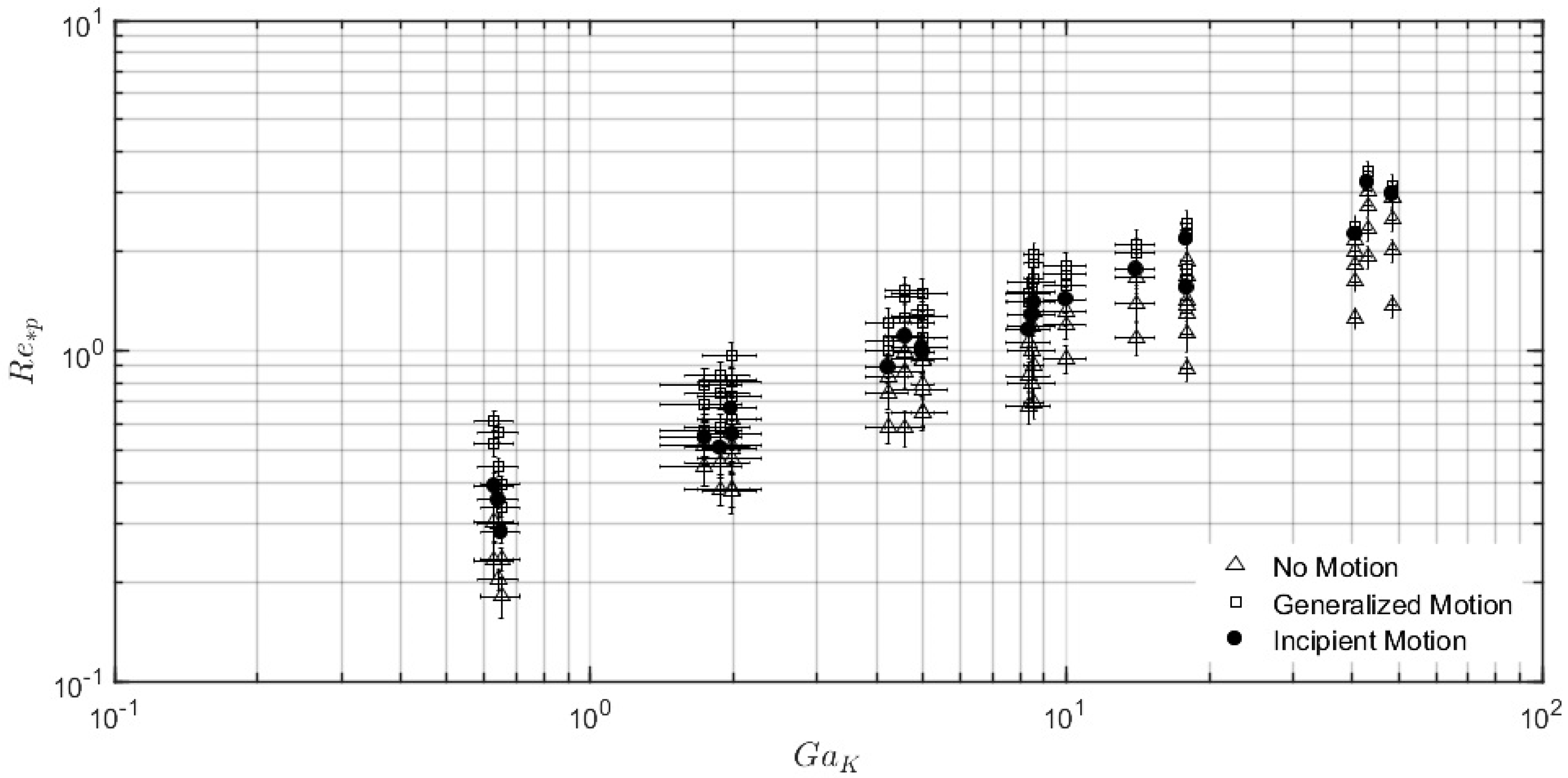
In a first analysis, it is assumed that ${\Phi }_3\left(n,G{a}_K\right)={\Phi }_4\left(G{a}_K\right)$, i.e., the effect of $n$ is well represented in the exponents of the different variables involved in the definition of the modified Galileo number $G{a}_K$. Thus, the condition for incipient motion is given by the functional relationship $R{e}_{*P}={\Phi }_4\left(G{a}_K\right)$, which is presented in Figure 3. In the figure, the data corresponding to the conditions of “no motion” and “generalized motion” are also included. The experimental data plotted in the figure include their associated error. The dispersion of the experimental points, particularly those corresponding to the incipient motion condition, is within the experimental error and cannot be attributed to an effect of the flow index. Thus, the assumption that the incipient condition can be represented by a relation between only $R{e}_{*P}$ and $G{a}_K$, is a valid one.

5. Discussion

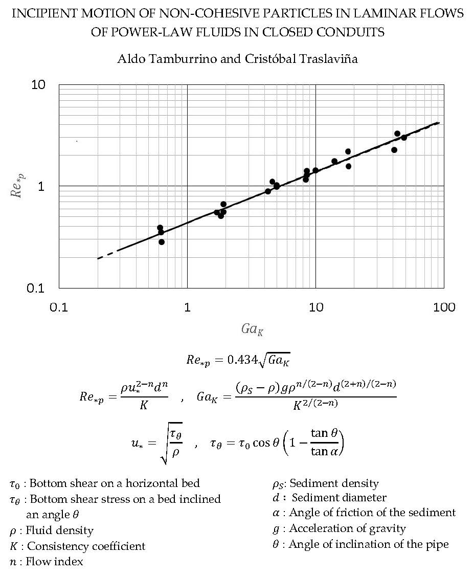
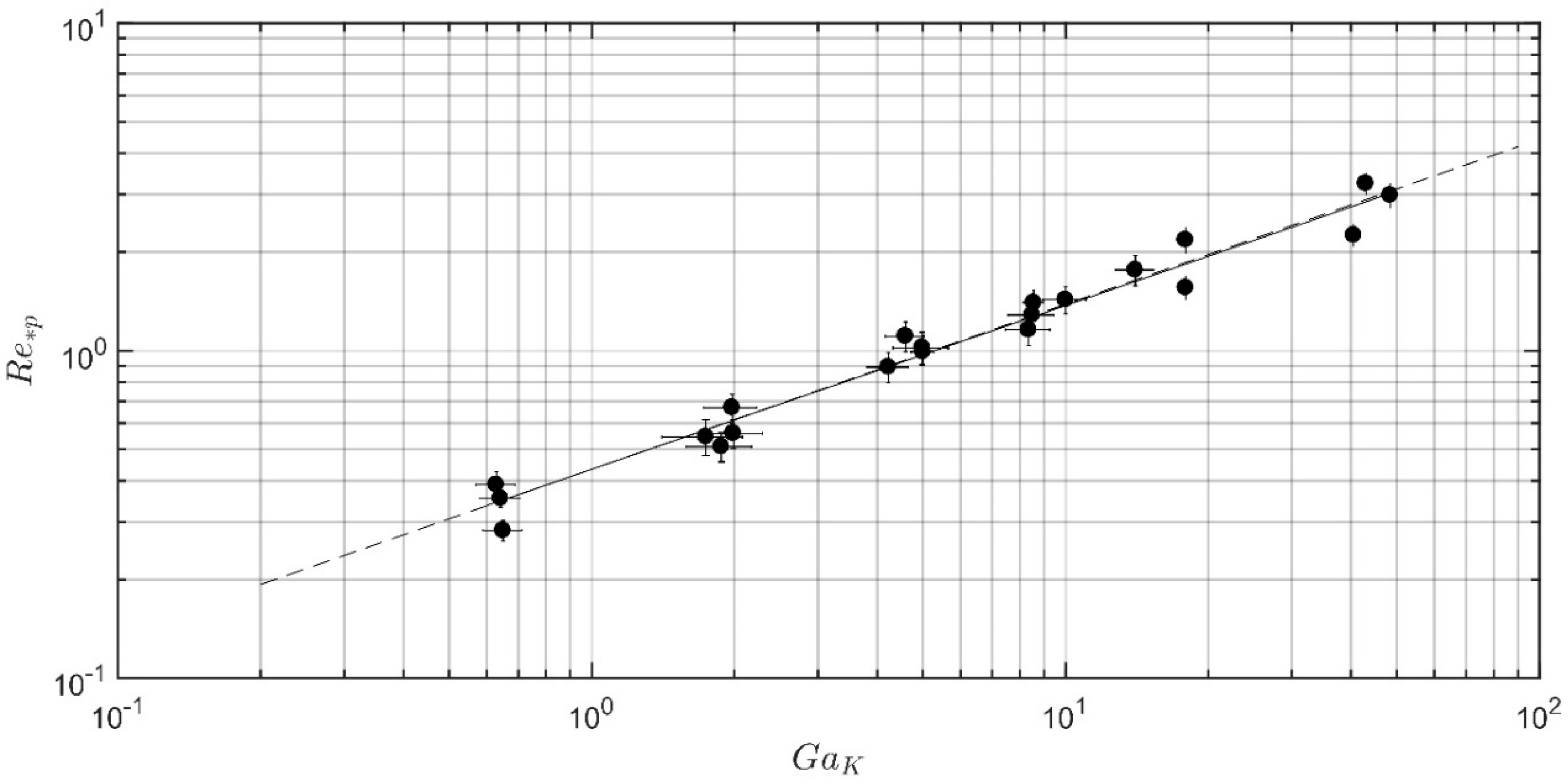
In order to have a clearer image of the data corresponding to incipient motion, only the points associated to this condition are shown in Figure 4, including the best fitting curve (continuous line), which is given by $R{e}_{*p}=0.434G{a}_K{}^{0.504}$, with a correlation coefficient $R^2=0.97185$. A second, segmented line, almost undistinguishable from the previous one, is also plotted in the figure. This line is a fit to the data, forcing a square root relationship between $R{e}_{*p}$ and $G{a}_K$. Thus, the condition of incipient motion of non-cohesive sediments due to the flow of a power-law fluid in a closed conduit is considered to be given by (with $R^2=0.97176$):

$$R{e}_{*p}=0.434\sqrt{G{a}_K}$$

(14)

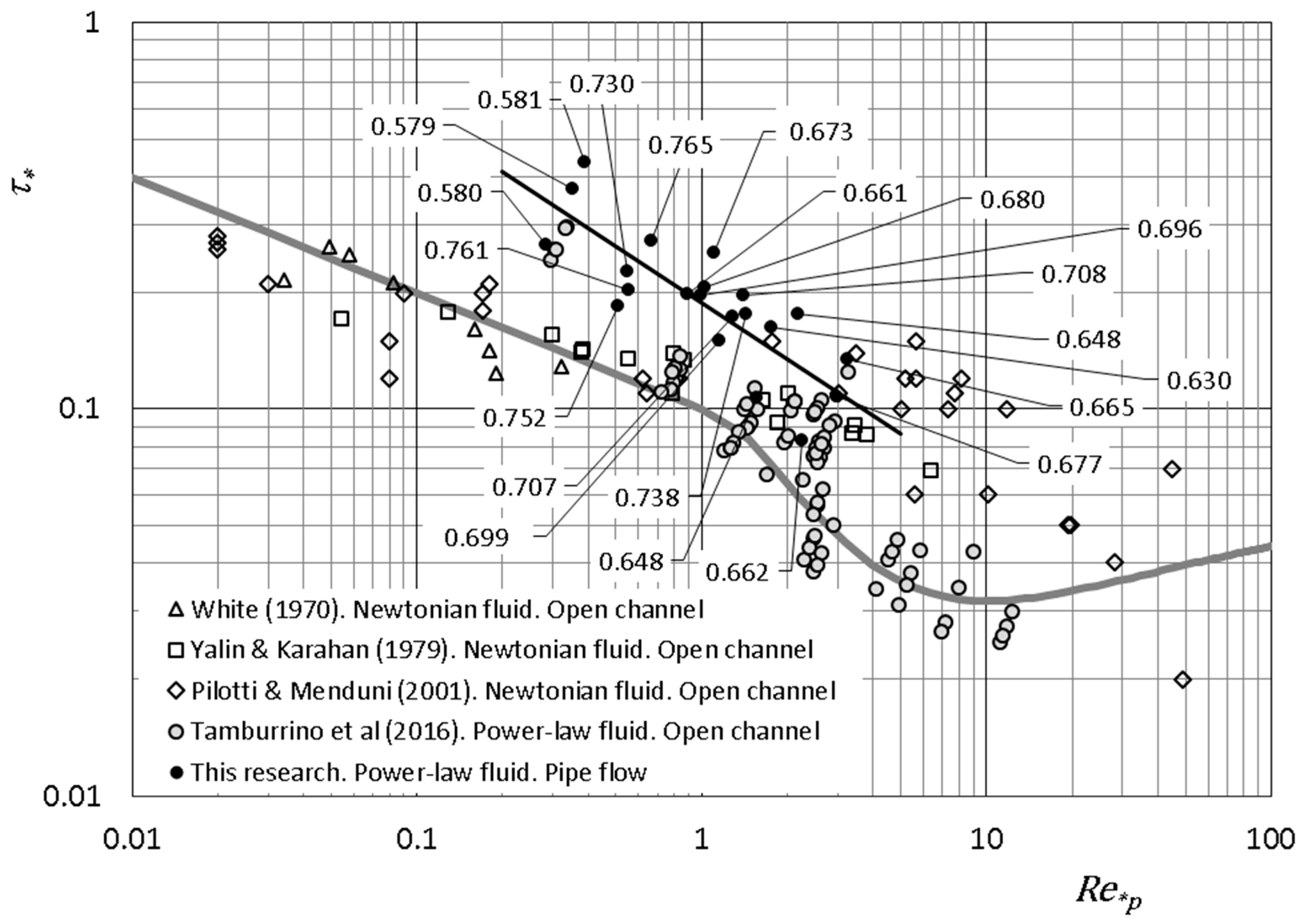
Figure 5 presents the experimental data in the standard plot of the pairs ${\tau }_{*}={\tau }_0/\left(\left({\rho }_S-\rho \right)gd\right)$ and $R{e}_{*}$, first envisaged by Shields [7] and popularized by Rouse [8]. It includes some results obtained by other researchers in open-channel laminar flows, for Newtonian fluids (mostly water), and the data by Tamburrino et al. [6], who worked with aqueous solutions of CMC and carbopol, which presented a power-law rheology. It is easy to show that the modified particle Reynolds number becomes the usual one when applied to Newtonian fluids, i.e., $n=1$, and $K=\mu$, the dynamic viscosity. The data by White (1970) appear tabulated in [12], from where they were taken for the plot. The continuous line corresponds to the incipient motion condition defined by Rouse [8] for $R{e}_{*}>1$, and Mantz [12] for $R{e}_{*}<1$.

The data present a larger scatter when they are plotted in the Shields diagram (Figure 5) instead of a $R{e}_{*}$ versus $G{a}_K$ plot (Figure 4). This is a common feature of the Shields diagram, already discussed elsewhere [9,33]. The critical Shields stress corresponding to pipe flow is higher than the measurements obtained, also for power-law fluids, in open channels, and higher than the Rouse–Mantz curve for incipient condition. Although the results obtained in this research are within the general dispersion of the rest of the data, and they seem to follow the tendency and dispersion of Pilotti and Menduni’s data [14] in open channels, it is not clear that ours can be entirely attributed to the subjectivity of the criterion used to define the condition of incipient motion. It has to be noted that higher critical Shield stresses have also been reported for turbulent flows in closed conduits by Chiew and Parker [34], but the reason this happens remains unclear.

The plot presented in Figure 4, which gives the condition of incipient motion in terms of the modified particle Reynolds and Galileo numbers, can be transformed into a Shields diagram in order to present our data in Figure 5. It can be shown that the dimensionless critical shear stress, ${\tau }_{*}$ is related to $R{e}_{*}$ and $G{a}_K$ by means of ${\tau }_{*}=R{e}_{*}^{2/\left(2-n\right)}/G{a}_K$. To see if the data segregate according to their non-linearity (given by the flow index), in such a way that those with higher values of $n$ lay closer to the Rouse–Mantz curve, and data with smaller $n$ are located farther, all the experimental points were labeled with their $n$ value. It is observed that no evident tendency exists, as all the data mingle independently of $n$. Thus, using Equation (14), ${\tau }_{*}=0.188R{e}_{*}^{-\left(2-2n\right)/\left(2-n\right)}$ is obtained. This relation is plotted in Figure 5 (black straight line) for $n=-0.487$, corresponding to the average value of the flow index of the CMC aqueous solutions used in the experiments.

6. Conclusions

The condition of incipient motion of non-cohesive granular particles due to the laminar flow in an inclined closed conduit of a power-law fluid can be defined in terms of two dimensionless parameters, properly modified to take into account the non-Newtonian characteristic of the fluid: a particle Reynolds number ($R{e}_{*}$) and a Galileo number ($G{a}_K$). The slope of the pipe is considered in the Reynolds number through the friction velocity, which is computed from the effective shear acting on the particle, modified to include the bed slope and angle of friction of the sediments. It is shown that the parameter obtained from dimensional analysis, identified as the Galileo number, effectively represents the ratio between the particle buoyancy and the shearing, non-Newtonian, viscous force acting on the sediment. Although the dimensional analysis indicates that the condition of incipient motion should also depend, in addition to $R{e}_{*p}$ and $G{a}_K$, on the flow index, $n$, it is not possible to elucidate its effect from the experimental data obtained in this research. Thus, the mode of incipient motion is well represented by a relation between the particle Reynolds number and the square root of the Galileo number.

The data, presented in a Shields diagram, show a large scatter, but they are in the range of dispersion of the data obtained in other research, also for laminar flow but in open channels, which include Newtonian and power-law fluids.

References

- Pal, R. Rheology of Particulate Dispersions and Composites; CRC Press: Boca Raton, FL, USA, 2007. [Google Scholar]
- Coussot, P.; Ancey, C. Rheophysical classification of concentrated suspensions and granular pastes. Phys. Rev. E 1999, 59, 4445. [Google Scholar] [CrossRef]
- Coussot, P.; Meunier, M. Recognition, classification and mechanical description of debris flows. Earth-Sci. Rev. 1996, 40, 209. [Google Scholar] [CrossRef]
- Ihle, C.F.; Tamburrino, A.; Montserrat, S. Identifying the relative importance of energy and water costs in hydraulic transport systems through a combined physics- and cost-based indicator. J. Cleaner Prod. 2014, 84, 589–596. [Google Scholar] [CrossRef]
- Wasp, E.J.; Kenny, J.P.; Gandhi, R.L. Solid-Liquid Flow Slurry Pipeline Transportation, 1st ed.; Trans Tech Publications: Clausthal, Germany, 1977. [Google Scholar]
- Tamburrino, A.; Carrillo, D.; Negrete, F.; Ihle, C. Critical shear stress for incipient motion of non-cohesive particles in open channel flows of pseudoplastic fluids. Can. J. Chem. Eng. 2016, 94, 1084–1091. [Google Scholar] [CrossRef]
- Shields, A. Anwendung der Ähnlichkeitsmechanik und der Turbulenzforschung auf die Geschiebebewegung. In Mitteilungen der Preussischen Versuchsanstalt für Wasserbau und Schiffbau; Ott, W.C., van Uchelon, J.C., Eds.; Cooperative Laboratory, Institute of Technology: Pasadena, CA, USA, 1936. [Google Scholar]
- Rouse, H. An Analysis of Sediment Transportation in Light of Fluid Turbulence, Sediment Division; Report No. SCS-TP-25; U.S. Department of Agriculture, Soil Conservation Service: Washington, DC, USA, 1939.
- Buffington, J.; Montgmery, D.R. A systematic analysis of eight decades of incipient motion studies, with special reference to gravel-bedded rivers. Water Resour. Res. 1997, 33, 1993–2029. [Google Scholar] [CrossRef] [Green Version]
- Dey, S.; Papanicolaou, A. Sediment Threshold under Stream Flow: A State-of-the-Art Review. KSCE J. Civil Eng. 2008, 12, 45–60. [Google Scholar] [CrossRef]
- White, J. Plane bed thresholds of fine grained sediments. Nature 1970, 228, 152–153. [Google Scholar] [CrossRef]
- Mantz, P.A. Incipient transport of fine grains and flakes by fluids–Extended Shields diagram. J. Hyd. Div. ASCE 1977, 103, 601–615. [Google Scholar]
- Yalin, M.S.; Karahan, E. Inception of sediment transport. J. Hyd. Div. ASCE 1979, 105, 1433–1443. [Google Scholar]
- Pilotti, M.; Menduni, G. Beggining of sediment transport of incoherent grains in shallow shear flows. J. Hyd. Res. 2001, 39, 115–124. [Google Scholar] [CrossRef] [Green Version]
- Cheng, N.-S. Analysis of bedload transport in laminar flows. Adv. Water Res. 2004, 27, 937–942. [Google Scholar] [CrossRef]
- Kuru, W.C.; Leighton, D.T.; McCready, M.J. Formation of waves on a horizontal erodible bed of particles. Int. J. Multiphase Flow 1995, 21, 1123–1140. [Google Scholar] [CrossRef]
- Loiseleux, T.; Gondret, P.; Rabaud, M.; Doppler, D. Onset of erosion and avalanche for an inclined granular bed sheared by a continuous laminar flow. Phys. Fluids 2005, 17, 103304. [Google Scholar] [CrossRef]
- Ouriemi, M.; Aussillous, P.; Medale, M.; Peysson, Y.; Guazzelli, E. Determination of the critical Shields number for particle erosion in laminar flow. Phys. Fluids 2007, 19, 061706. [Google Scholar] [CrossRef] [Green Version]
- Lobkovsky, A.E.; Orpe, A.B.; Molloy, R.; Kudrolli, A.; Rothman, D.H. Erosion of granular bed driven by laminar fluid flow. J. Fluid Mech. 2008, 605, 47–58. [Google Scholar] [CrossRef] [Green Version]
- Rabinovich, E.; Kalman, H. Incipient motion of individual particles in horizontal particle–fluid systems: A. Experimental analysis. Powder Tech. 2009, 192, 318–325. [Google Scholar] [CrossRef]
- Hong, A.; Tao, M.; Kudrolli, A. Onset of a granular bed in a channel driven by a fluid flow. Phys. Fluids 2015, 27, 013301. [Google Scholar] [CrossRef] [Green Version]
- Charru, F.; Mouilleron-Arnould, H. Instability of a bed of particles sheared by a viscous flow. J. Fluid Mech. 2002, 452, 303–323. [Google Scholar] [CrossRef]
- Charru, F.; Hinch, E.J. Ripple formation on a particle bed sheared by a viscous liquid. Part 1. Steady flow. J. Fluid Mech. 2006, 550, 111–121. [Google Scholar] [CrossRef] [Green Version]
- Ouriemi, M.; Aussillous, P.; Guazzelli, E. Sediment dynamics. Part 1. Bed-load transport by laminar shearing flows. J. Fluid Mech. 2009, 636, 295–319. [Google Scholar] [CrossRef] [Green Version]
- Daido, A. On The Occurrence of Mud-Debris Flow. Bull. Disas. Prey. Res. 1971, 21, 109–135. [Google Scholar]
- Wan, Z. Bed material movement in hyperconcentrated flow. J. Hyd. Eng. ASCE 1985, 111, 987–1002. [Google Scholar] [CrossRef]
- Kim, S.C.; Oh, K.S.; Kim, Y.J.; Irvine, T.F., Jr.; Yamasaki, T. Hydrodynamic Entrance Lengths and Entrance Correction Factors for a power-law Fluid in a Circular Duct. Korean J. Rheol. 1995, 7, 261–266. [Google Scholar]
- Dodge, D.W.; Metzner, A.B. Turbulent flow of non-Newtonian systems. AIChE J. 1959, 5, 189–204. [Google Scholar] [CrossRef]
- Kozicki, W.; Chou, C.H.; TIU, C. Non-Newtonian flow in ducts of arbitrary cross-sectional. Chem. Eng. Sci. 1966, 21, 665–679. [Google Scholar] [CrossRef]
- Granger, R.A. Fluid Mechanics, 1st ed.; Dover Publications, Inc.: New York, NY, USA, 1995. [Google Scholar]
- Berendsen, H. A Student’s Guide to Data and Error Analysis; Cambridge University Press: Cambridge, UK, 2011. [Google Scholar]
- Taylor, J.R. An Introduction to Error Analysis; University Science Books: Sausalito, CA, USA, 1997. [Google Scholar]
- Simões, F.J.M. Shear velocity criterion for incipient motion of sediment. Water Sci. Eng. 2014, 7, 183–193. [Google Scholar]
- Chiew, Y.-M.; Parker, G. Incipient sediment motion on non-horizontal slopes. J. Hyd. Res. 1994, 32, 649–660. [Google Scholar] [CrossRef]
Figure 1.
Sketch of the experimental setup.
Figure 2.
Rheogram corresponding to the water- sodium carboxymethyl cellulose (CMC) solution used in Experiment 13. The solid line is the best fitting curve to the measurements, given by , with a correlation coefficient .
Figure 3.
Relation between the modified particle Reynolds number and the modified Galileo number. Error bars are also included.
Figure 4.
Condition of incipient motion in terms of the modified particle Reynolds number and the modified Galileo number. Continuous line corresponds to the best fit of the data. Segmented line is the relationship .
Figure 5.
Condition of incipient motion presented in the standard Shields diagram with data corresponding to laminar flows of Newtonian and power-law fluids. The grey line is the Rouse–Mantz fitting to the movement threshold condition. The experimental points corresponding to the incipient condition in a pipe flow (this research, black filled circles) show the value of the flow index. The black line is the threshold condition obtained from Equation (14).