Evaluation of Snowmelt Estimation Techniques for Enhanced Spring Peak Flow Prediction

1
School of Geography and Earth Sciences, McMaster University, 1280 Main Street West, Hamilton, ON L8S 4K1, Canada
2
Department of Civil Engineering, McMaster University, 1280 Main Street West, Hamilton, ON L8S 4L7, Canada
3
United Nations University Institute for Water, Environment, and Health, Hamilton, ON L8P 0A1, Canada
*
Author to whom correspondence should be addressed.
Water 2020, 12(5), 1290; https://doi.org/10.3390/w12051290
Submission received: 4 April 2020
/
Revised: 29 April 2020
/
Accepted: 30 April 2020
/
Published: 1 May 2020
(This article belongs to the Section Hydrology)
Abstract
:Water resources management and planning requires accurate and reliable spring flood forecasts. In cold and snowy countries, particularly in snow-dominated watersheds, enhanced flood prediction requires adequate snowmelt estimation techniques. Whereas the majority of the studies on snow modeling have focused on comparing the performance of empirical techniques and physically based methods, very few studies have investigated empirical models and conceptual models for improving spring peak flow prediction. The objective of this study is to investigate the potential of empirical degree-day method (DDM) to effectively and accurately predict peak flows compared to sophisticated and conceptual SNOW-17 model at two watersheds in Canada: the La-Grande River Basin (LGRB) and the Upper Assiniboine river at Shellmouth Reservoir (UASR). Additional insightful contributions include the evaluation of a seasonal model calibration approach, an annual model calibration method, and two hydrological models: McMaster University Hydrologiska Byrans Vattenbalansavdelning (MAC-HBV) and Sacramento Soil Moisture Accounting model (SAC-SMA). A total of eight model scenarios were considered for each watershed. Results indicate that DDM was very competitive with SNOW-17 at both the study sites, whereas it showed significant improvement in prediction accuracy at UASR. Moreover, the seasonally calibrated model appears to be an effective alternative to an annual model calibration approach, while the SAC-SMA model outperformed the MAC-HBV model, no matter which snowmelt computation method, calibration approach, or study basin is used. Conclusively, the DDM and seasonal model calibration approach coupled with the SAC-SMA hydrologic model appears to be a robust model combination for spring peak flow estimation.
1. Introduction
Accurate time- and site- specific spring flood forecasting is essential for water resources management and planning [1]. Reliable spring flow predictions are needed by operators of hydropower reservoirs as well as by water resources managers. They also hold considerable economic value through enhanced operational decision making, efficient hydroelectric power generation, reduced downstream flood occurrences, and better managed hydraulic structures. Despite these advantages, reliable spring flow prediction remains challenging. A few techniques that can be adopted for improving the spring flow prediction accuracy include: 1) enhancing meteorological forecast and hydrometric input data (i.e., different input forcing [1,2]); 2) improving optimization techniques (i.e., different approaches to obtain optimal model parameters [3,4]); 3) using multi-models (i.e., use different models and inter-compare their performances [5,6,7]) and 4) Modifying complexity of physical processes governing the hydrologic model structure (e.g., snowmelt routing or other representative water balance component [4,5,7,8,9]). Our focus herein is to investigate and analyze approaches 2), 3), and particularly 4).
Spring snowmelt freshet is the major cause of floods in the snow-dominated watersheds [1,10]. This implies the need for accurate and robust snowmelt computation methods [8,11,12]. To determine snowmelt, various computational methods have been proposed ranging from simple temperature index methods to complex and multi-layered energy budget models and hybrids between these two methods [8,11,12,13]. Recent reviews of snowmelt estimation methods [14,15] and advances in the snow model intercomparison studies can be found in [11,16,17,18]. Snow models examined in this study are temperature-index models as they require only precipitation and temperature data, while an energy budget approach requires additional data inputs such as radiation, wind, and humidity, that are not generally available at mountainous sites [19]. Furthermore, the empirically-based degree-day method demonstrates similar, and often better, performance than physically based energy balance models [7,8,9,20,21]. Despite the effectiveness, simplicity, applicability, and accuracy of the degree-day method, it is frequently suggested to replace the method with more complex approaches to improve the accuracy of snowmelt estimates and subsequent reservoir inflow predictions [8,9,22,23]. SNOW-17, a more sophisticated process-based model used operationally by the National Weather Service (NWS) to produce snow accumulation and melt forecasts in snow-dominated catchments across the United States, is used herein to investigate its effectiveness against the popular degree-day method.
In operational snow hydrology, in addition to assessing the benefits of one snow model over another, model parameter optimization is an important decision that affects the accuracy and performance of the hydrologic modeling system [3,4]. Robust model calibration process depends on the selection of representative calibration data, appropriate objective functions, and optimization algorithms, of which identifying a representative data set is a crucial factor and forms the basis of the optimization process [4]. Annual models are calibrated to minimize the error between observed and simulated inflows throughout the year, which can be computationally inefficient if extreme hydrologic events are of primary interest. An alternative approach is to consider seasonal time series of interest (herein spring season) in which parameters are adjusted to match specifically the recorded seasonal flows. This can lead to efficiency in terms of time, computational cost, and accuracy. Given the potential advantages of using seasonal models, a particular interest of the study is to assess the effectiveness of seasonal models.
Among the studies on snowmelt models, many studies have compared the performance of temperature index methods or their extended versions with energy balance models or their variants [6,7,8,11,16,17,18,24,25,26]. Very few studies have focused on comparing empirical and conceptual snowmelt models [7,16]. However, those studies did not aim at comparing the performance of snowmelt models specifically to improve spring peak flow prediction. The objective of this study is to investigate the potential of two popular snowmelt models, the degree-day method (DDM) and the more complex SNOW-17 model, to improve the spring peak flow prediction in snow-dominated watersheds. A second objective of the study is to evaluate the potential of seasonal model calibration approaches to enhance flood prediction as compared to annual model calibration methods using an advanced global optimization algorithm. Subsequently, the aim is to identify and assess the hydrological model performance and their model combinations thereof for improved spring flood prediction.
To achieve the aforementioned objectives, two hydrologic models (MAC-HBV and SAC-SMA) are used in conjunction with two snowmelt estimation methods (DDM and SNOW-17 model) and two calibration approaches (seasonal and annual) leading to eight model structures. These model combinations were implemented at two snow-dominated watersheds in Canada, one of which has a hydrologically complex terrain. The remainder of this paper is structured as follows: Section 2 describes the study area and data. Section 3 presents the methodology, including a brief description of the models, snowmelt estimation procedures, model optimization, and evaluation. Results and discussion are then presented in Section 4 and Section 5, respectively. Finally, the conclusions are reported in Section 6.
2. Materials
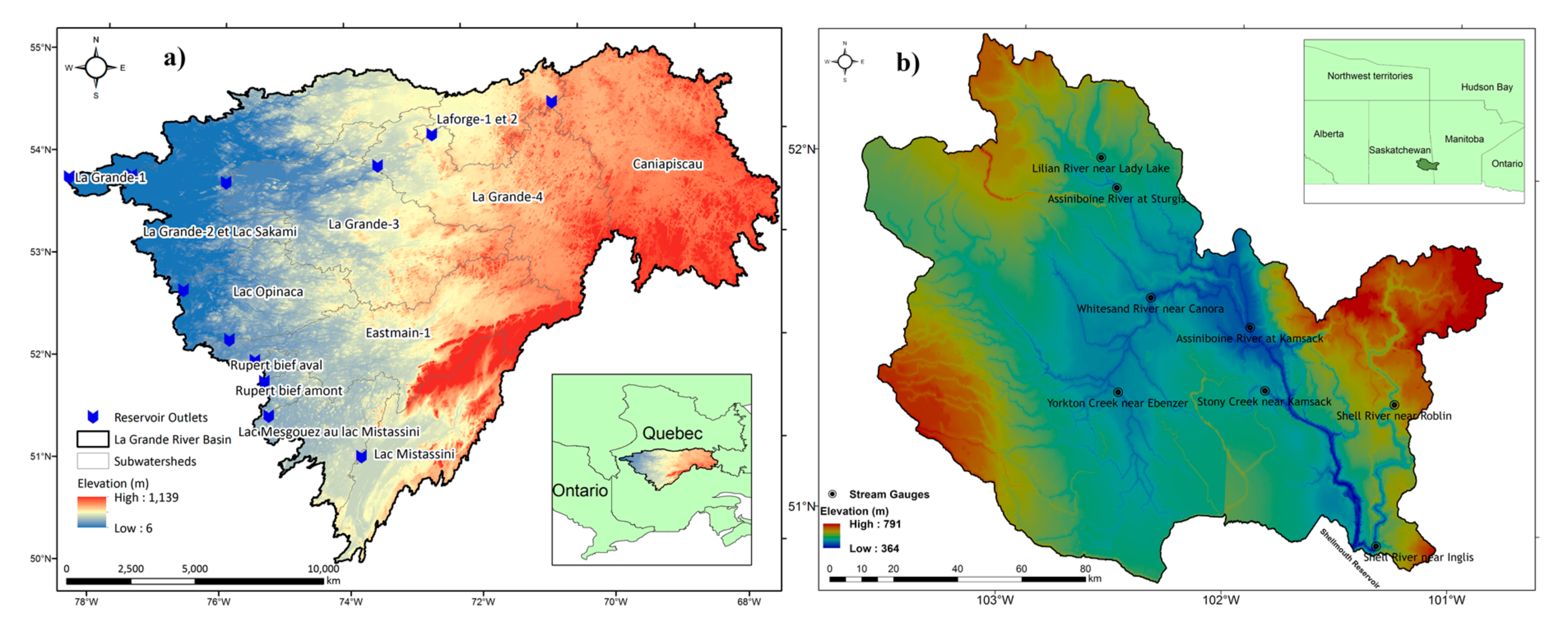
The study was conducted on two watersheds in Canada: the La-Grande River Basin (LGRB) in the Province of Quebec, and Upper Assiniboine river at Shellmouth Reservoir (UASR) in the Province of Manitoba. The LGRB is in north-central Quebec (Figure 1a) and contains the James Bay Hydroelectric Complex. A portion of the Caniapiscau, Opinaca, and Eastmain river flows were diverted to the La-Grande River [27]. The present research includes La-Grande River and the diverted sub-watersheds, combined they are referred to as La-Grande River Basin (Figure 1a). The basin has a total drainage area of nearly 209,000 km2 including the diverted basins and is primarily covered by forests (97%) and secondarily by water bodies (3%) [28]. According to the Canadian Climate Normals (1981–2010) at La-Grande River (53°38’N, 77°42’W), the mean annual precipitation is 697 mm out of which more than one-third is snowfall. Thus, peak runoff due to spring snowmelt is evident in the basin hydrology. The average temperature ranges between −28 °C to −8 °C in winter (Jan–Mar) and −10 °C to 17 °C in spring (Apr–Jun).
LGRB consists of 12 sub-catchments with each of its sub-basin containing a reservoir managed by Hydro-Quebec. The observed historical total precipitation, maximum and minimum temperatures, and reservoir inflows were obtained on a daily timescale for 36 years (1970–2005) from Hydro-Quebec. Different sub-basins comprised of varying data lengths. The two sub-basins that have more than 90% missing values were excluded from the study. Of the remaining 10 sub-watersheds, one had 32 years of data, two had 22 years, and seven had between five and nine years of data. Calibration was conducted at lumped sub-basin scale at reservoir inflow of each sub-basin. The model was calibrated and validated for the precipitation, temperature, and streamflow time series consisting of non-missing values to ensure proper training and testing of the models.
The second study area is the Upper Assiniboine river at Shellmouth Reservoir (Lake of the Prairies Reservoir) located along the Saskatchewan-Manitoba border, with a gross drainage area of nearly 18,300 km2 (Figure 1b). The majority of this watershed lies in the prairie pothole region of the Canadian Prairies [29]. For a detailed understanding of the complex hydrology of the prairie pothole region, the interested reader is referred to [10,29,30]. Based on 1981–2010 data, air temperature varies seasonally between −22 °C to −1.4 °C in winter (Jan-Mar) and −2.6 °C to +21.8 °C in spring (Apr–Jun), with about 511 mm of mean annual precipitation. UASR was selected for the experiment as it is a snow-dominated watershed with more than 80% of the total annual flow occurring during the spring snowmelt season [30,31]. The observed daily precipitation and temperature data were obtained from Environment Canada for the 23 years (1994–2015) period, while streamflow and reservoir inflow time series for the same period was provided by the Hydrologic Forecast Centre, Manitoba Infrastructure (MI). Calibration was conducted at Shellmouth reservoir inflow and one of the major gauging stations feeding the reservoir, the Assiniboine river at Kamsack station.
3. Methods
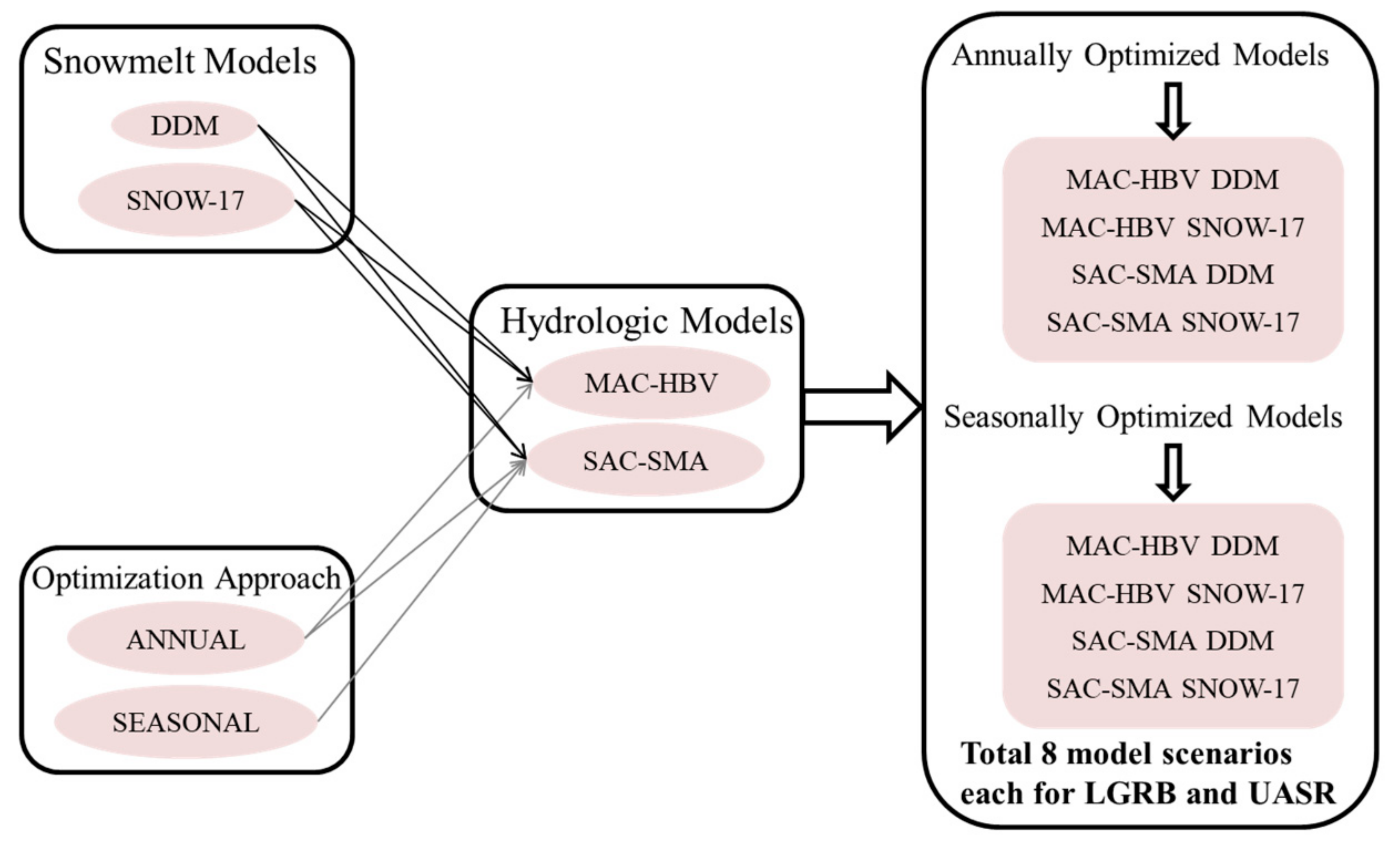
In this study, two hydrological models (MAC-HBV and SAC-SMA) along with two snowmelt estimation techniques (DDM and SNOW-17), and calibration approaches (annual and seasonal calibration) were investigated. This resulted in four model structures namely, MAC-HBV DDM, MAC-HBV SNOW17, SAC-SMA DDM and SAC-SMA SNOW17, each for LGRB and UASR. Additionally, as shown in Figure 2, we used annual and seasonal parameter optimizations which we refer to as annually and seasonally optimized models. Each method is described in further detail in the following sub-sections.
3.1. Hydrological Models
3.1.1. MAC-HBV Model
The McMaster University Hydrologiska Byrans Vattenbalansavdelning (MAC-HBV) model is a lumped conceptual rainfall-runoff model [32] that follows the structure of HBV [33]. The model has been successfully applied in a wide range of hydrological studies [34,35,36], including peak flow forecast studies [1]. It includes a snow routine, soil moisture routine, a response function, and a routing routine. The meltwater obtained from the snowmelt estimation methods combined with rain is input to the soil moisture routine. Changes in soil moisture storage of the topsoil layer are represented by the soil moisture routine, and daily potential evapotranspiration is determined by a simplified form of Thornthwaite equation. Runoff contribution from the upper and lower zone soil reservoir is represented by the response function, after which equilateral triangular weighting function is utilized for channel routing to obtain the final streamflow.
The version of MAC-HBV used in this study is a semi-distributed variant of the model, i.e., it was optimized at the reservoir inflow of each sub-catchment for LGRB and at the Kamsack gauge station and reservoir inflow in UASR. The model requires daily precipitation and temperature time series as inputs to simulate daily flow. While the model adapted here is based on the daily scale, it is possible to reduce the temporal resolution of the model. The parameters calibrated herein, their description, and ranges for the models used in the study are summarized in Table 1.
3.1.2. SAC-SMA Model
The Sacramento Soil Moisture Accounting model (SAC-SMA) [41] is a lumped conceptual watershed model operationally implemented by United States’ National Weather Service River Forecast System (NWSRFS) for streamflow predictions and flood forecasts [34]. It has been extensively used in previous studies in snowy regions [37,42,43]. SAC-SMA treats precipitation that occurs on pervious and impervious areas separately and treats accumulation in the upper and lower soil zone reservoirs as “tension” and “free” waters, respectively, for precipitation on pervious areas, or as direct runoff otherwise. The inputs to the model include daily precipitation and temperature time series, while it simulates the channel inflow, which is converted to streamflow using a simple Nash Cascade routing approach comprising of three linear reservoirs. The snowmelt component and evapotranspiration estimation used here are the same as the MAC-HBV model. Although SAC-SMA is a lumped model, it was adapted in a semi-distributed manner calibrating at reservoir inflow of each sub-watershed for LGRB and at Kamsack flow station and reservoir inflow for UASR.
3.2. Snowmelt Estimation Methods
3.2.1. Degree-Day Method
The degree-day method (DDM) is a temperature index approach that uses a relationship between snowmelt and air temperature to obtain melt rate [22,23,44]. DDM has evolved since its inception several decades ago [9,20,22] varying in complexity from simple index models to extended versions that are referred to as simplified energy balance models [22]. Extended DDM generally incorporates either radiation components in empirical form or considers seasonally variable degree day factors [22]. Despite these complexities accounted in the snow model, extended formulations often perform similar to simple DDM [7,8,22]. The variant of DDM used herein is similar to [32]. The melt rate (M) is computed as the product of temperature differences between mean daily air temperature (T) and melt temperature (Tm) (usually 0 °C) with degree-day factor (DDF). The melt equation is given by:
here, changes in snow water equivalent (SWE) are accounted as follows:
where, SCF is snow correction factor, Ps is snowfall (mm/day), Pm is rainfall (mm/day) and ∆t is time-step of a day. Rainfall and snowfall amounts are determined by upper and lower threshold temperatures distinguishing rain, snow and mix of snow and rain. Melt rate along with precipitation as rain is provided to hydrological model to obtain estimates of reservoir inflow.
3.2.2. SNOW-17 Model
SNOW-17 is a single-layer, process-based, temperature index model representing most of the complex physical processes occurring in the snow column [38,40]. The National Weather Service (NWS) produces operational snow accumulation and melt forecasts implementing SNOW-17 model for nationwide snow-dominated watersheds [13]. Since SNOW-17 model has demonstrated better prediction accuracy in many studies [13,45,46,47], it is used herein to compute snowmelt. SNOW-17 considers processes such as energy exchange at the snow-air interface, heat storage and heat deficit of the snowpack, liquid water storage and transmission, and also distinguish between rain-on-snow, rain-on-bare ground, and non-rain events to model snow accumulation and ablation [38]. Despite being a sophisticated model, the inputs are daily precipitation and daily temperature, which are readily available variables for most of the watersheds. It estimates outflow (snowmelt plus rain) and snow water equivalent (SWE), of which outflow is used as forcing to hydrological models. During rain-on-snow events, empirical energy balance equations are used to determine snowmelt utilizing several assumptions about meteorological conditions [38]. Whereas, the melt during non-rain periods (Mnr) is governed by melt factor and is described by:
where, Mf = seasonally varying melt factor, MBASE = Base temperature, fr = Fraction of precipitation in form of rain, Tr = Rain Temperature, Ta = Air temperature, P = Precipitation
3.3. Model Optimization
The optimization was performed to obtain a single set of best parameters that minimizes the error between observed and simulated streamflow. The four model combinations were calibrated for the even years considering the first year as spin-up and validated against the odd years. Annual as well as seasonal time series were optimized against the observed daily streamflow for the four model combinations. For the seasonal model training, spring months from March to July were considered in order to capture the rising limb and falling limb of the hydrograph. The seasonal model experiment was carried out to test the ability of seasonal models to provide better agreement between observed and computed inflows for the spring season. In a previous study, Particle Swarm Optimization algorithm (PSO) [48] has shown better performance in obtaining Pareto optimal set for hydrological models MAC-HBV and SAC-SMA, specifically in terms of reducing volume error of peak flows in Canadian watersheds [49]. Thus, PSO, a single objective, automatic global optimization algorithm was utilized herein to maximize the objective function NVE (Combined Nash-Sutcliffe efficiency and Volume error) [35] given by:
where the Nash-Sutcliffe efficiency (NSE) equation is as follows:
and volume error (VE) is calculated by:
The logarithm and square of NSE values can be expressed as:
where Qobs and Qsim are the observed and simulated streamflow values, respectively, is the average of observed streamflow values and N is the total number of data points. Equations (8) and (9) are similar to Equation (6) but they account for log-transformed flows and square-transformed flows and thus emphasize low flows and high flows, respectively. NSE spans between -∞ to 1 with 1 showing optimal performance for NSE and NVE. Inversely, VE ranges from 0 to ∞ and values closer to zero reveals better model performance. Using Equation (5), a single objective calibration approach can be used as a multi-objective approach. We repeated the calibration with objective function NVE (Equation (5)) to put more emphasis on high flows (NSEsqr). The recalibration was carried out for model combinations with the least performing sub-watersheds to check for improvement in performance, but we found that results did not improve peak flow statistics and hydrograph significantly. Henceforth, we include results obtained by training the models with the above objective function Equation (5).
3.4. Model Performance Criteria
The focus of this study is to assess improvement in spring peak flows; therefore, the model performance was evaluated for the spring season, i.e., April, May, and June months for the 8 model structures during the entire period of study. To assess the snowmelt estimation techniques (DDM and SNOW-17 model), model improvement metrics were used. Model improvement was calculated in terms of the percent reduction in the root mean squared error (RMSE, Equation (10)) when SNOW-17 model was adapted as compared to DDM (taken as base model for evaluation):
RMSE criterion is zero for a perfect model. Positive values of model improvement indicate better performance of the SNOW-17 model, while negative values reveal model deterioration due to the implementation of the SNOW-17 model. The evaluations were carried out for the spring season and for spring peak flow. Two criteria, namely NSE (Equation (6)) and Kling-Gupta Efficiency (KGE) [50] (Equation (11)) were used to assess the spring season model performance:
where ; ; . The optimal value of KGE is unity. To test the ability of the models to capture spring peak flow, generally a threshold is selected based on peak over threshold, flow duration percentile, or long-term median flow. In this study, we consider flows above the 75th percentile threshold to be high flows. This threshold was selected to have a similar number of peak flows for all the sub-watersheds to calculate error. Then, the RMSE and the Peak Flow Criteria (PFC, Equation (12)) were computed for flows over 75 percentile thresholds RMSE was computed using normalized streamflow to the area of each sub-watershed and thus termed normalized RMSE (NRMSE). PFC is considered a better performance indicator of prediction accuracy for the flood period and can be calculated as follows [51]:
where, is the number of peak flows greater than 75 percentile, and are the observed and predicted flows respectively. PFC value equal to zero represents optimal model performance.
The model performance evaluation criteria discussed above were computed using normalized streamflow to the area of each sub-watershed to be able to compare the sub-catchments with varying sizes.
4. Results
4.1. Evaluation of Snowmelt Estimation Methods: DDM and SNOW-17 Model
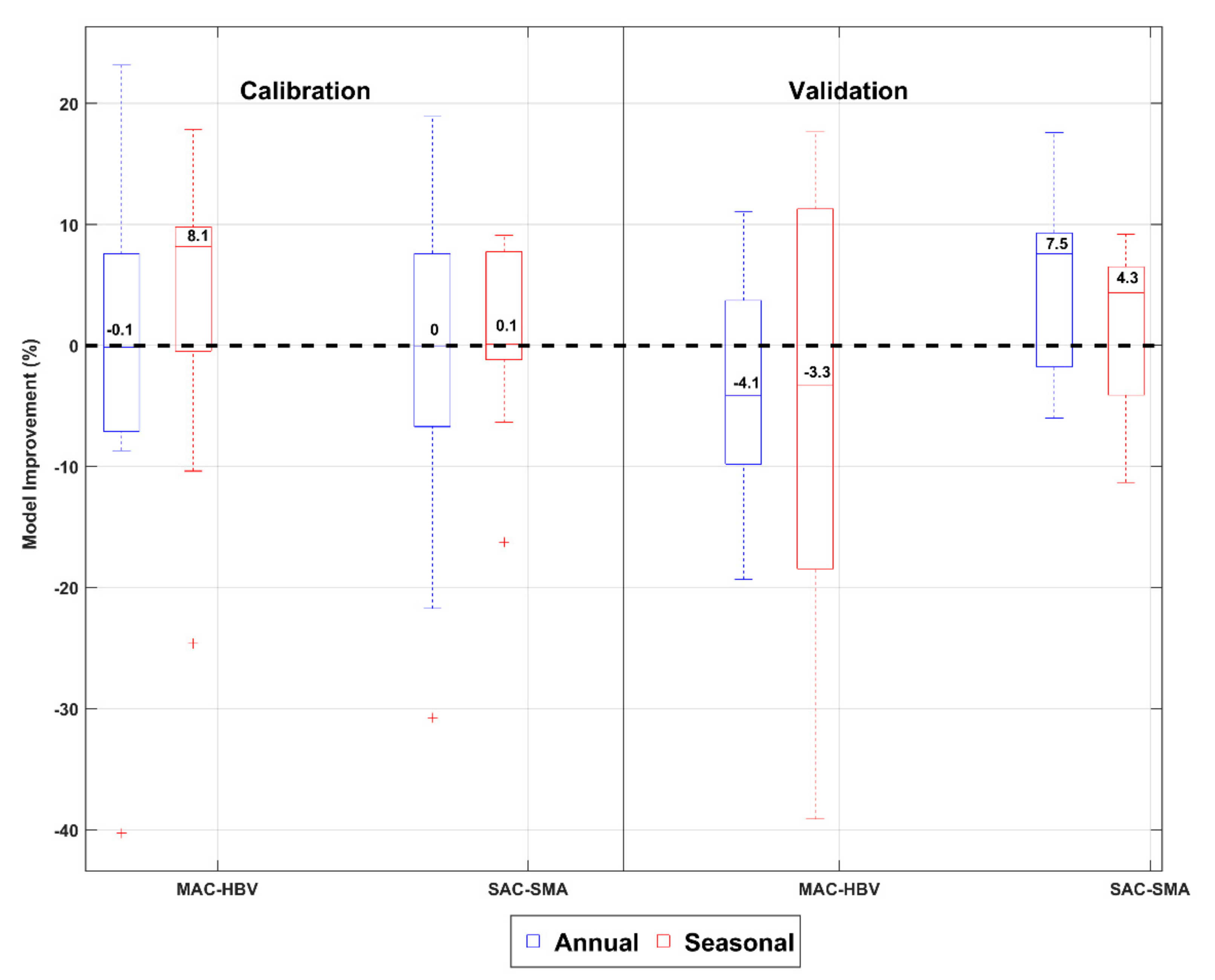
Model improvement of training and testing periods when the SNOW-17 model was used for the LGRB is presented in Figure 3. Recall that the positive percentages on the figure show improvement due to the implementation of the SNOW-17 model, and negative percentages show model deterioration due to the use of the SNOW-17 model. For instance, −0.1% model improvement during the testing period of annually calibrated MAC-HBV model structure indicates that the RMSE of annually optimized MAC-HBV-DDM is less than that of MAC-HBV-SNOW17 model. Therefore, model performance statistics deteriorated due to the use of the SNOW-17 model in the annually optimized MAC-HBV model. Similarly, the annual SAC-SMA-SNOW-17 model does not show any model improvement during the calibration period as the median model improvement is zero. The median of seasonal MAC-HBV-SNOW-17 model reveals improvement of about 8%, while the seasonal SAC-SMA model median does not show any model improvement during the testing period. For the validation period, model performance slightly deteriorates with the use of the SNOW-17 model in the annual MAC-HBV and seasonal MAC-HBV model structures. Whereas using the SNOW-17 model slightly improves the performance for the annual SAC-SMA and seasonal SAC-SMA model structures.
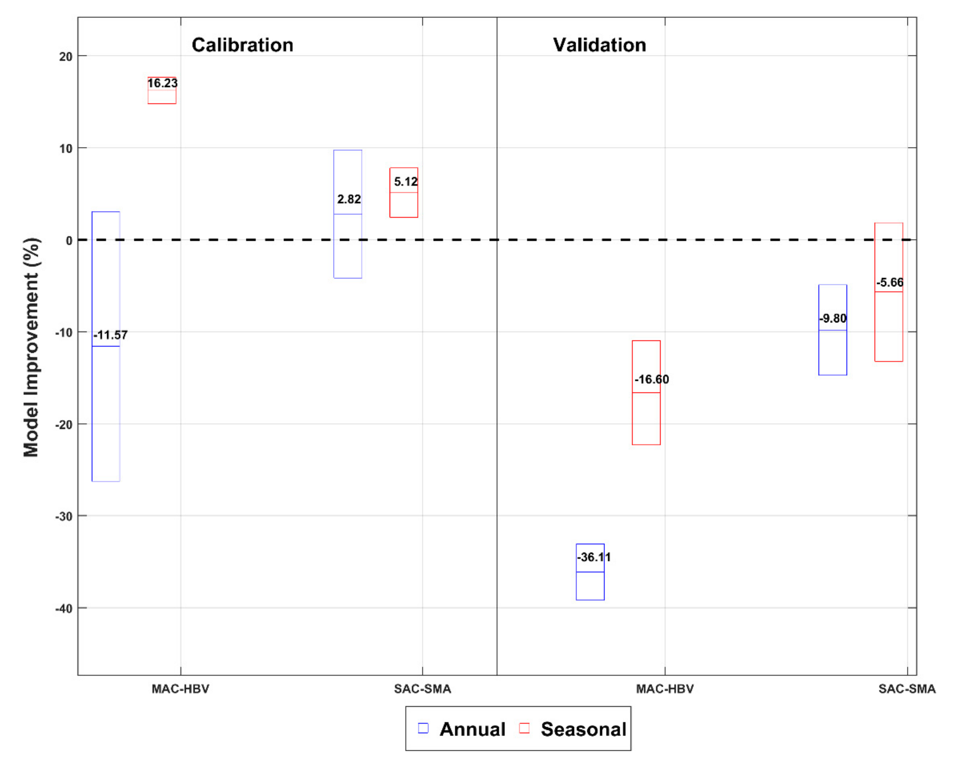
For instance, annual MAC-HBV and seasonal MAC-HBV model median deteriorated by about 4% and 3% when the SNOW-17 model was used. Whereas the medians of annual SAC-SMA and seasonal SAC-SMA models improved by ~7% and ~4% respectively with the SNOW-17 model. Overall, percentages for model improvement and deterioration due to the use of the SNOW-17 model (instead of DDM) are significantly lower, suggesting that SNOW-17 model use does not result in model performance improvement. The model improvement for UASR presented in Figure 4 depicts that using the SNOW-17 model improves the performance when coupled with seasonal MAC-HBV model, annual SAC-SMA, and seasonal SAC-SMA models during the calibration period. The model improvement varies between 2% and 16%. However, whatever optimization approach or hydrologic model is used, the SNOW-17 model deteriorates the model performance during the model verification period. For example, the median of model deterioration varies between ~5% to ~36% when using SNOW-17 for all model combinations. In general, in both the study areas and for the validation period, the median of six (out of eight) model scenarios show either model deterioration or no improvement due to the implementation of the SNOW-17 model. These results indicate that the DDM outperforms SNOW-17 for most model combinations in both study areas.
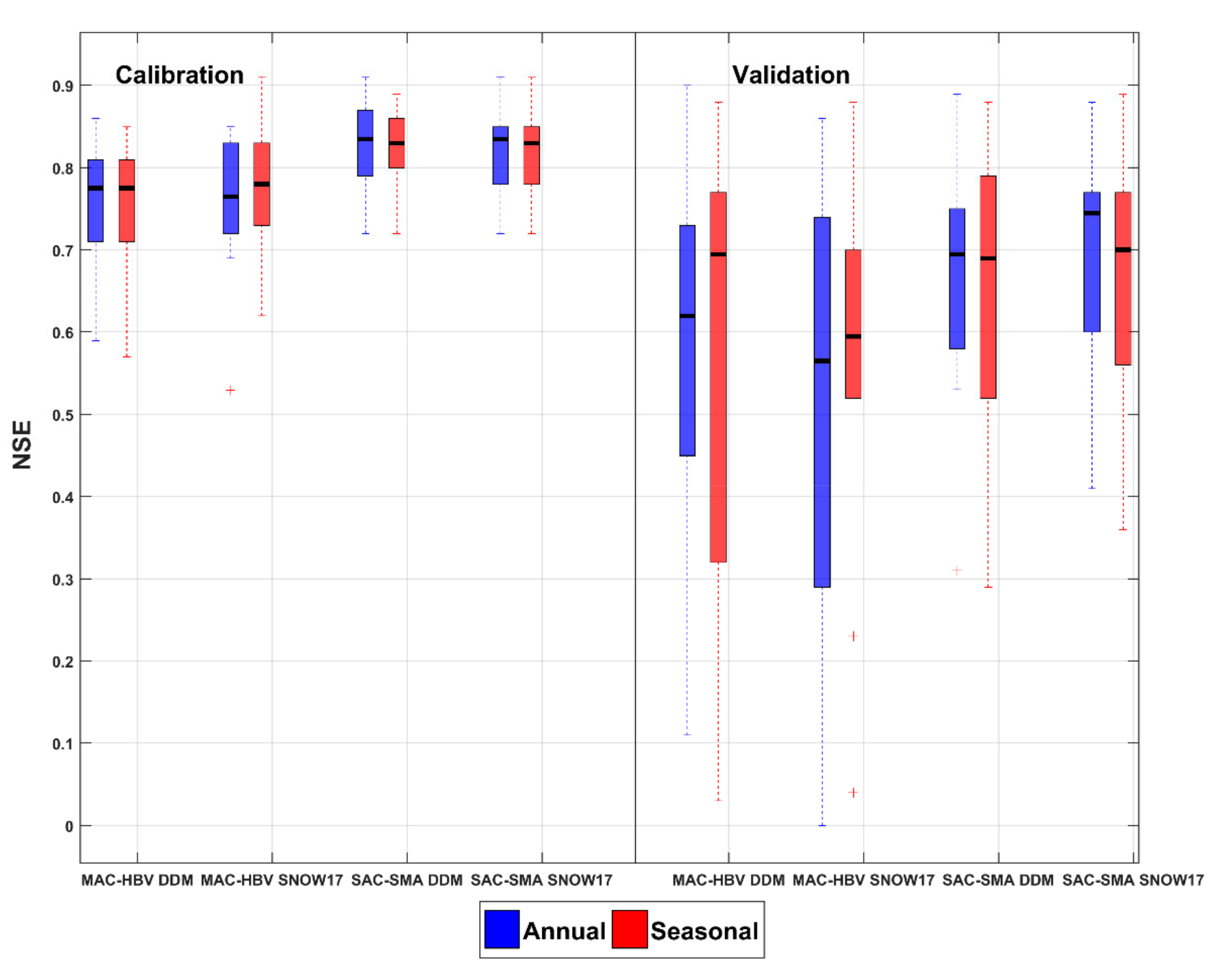
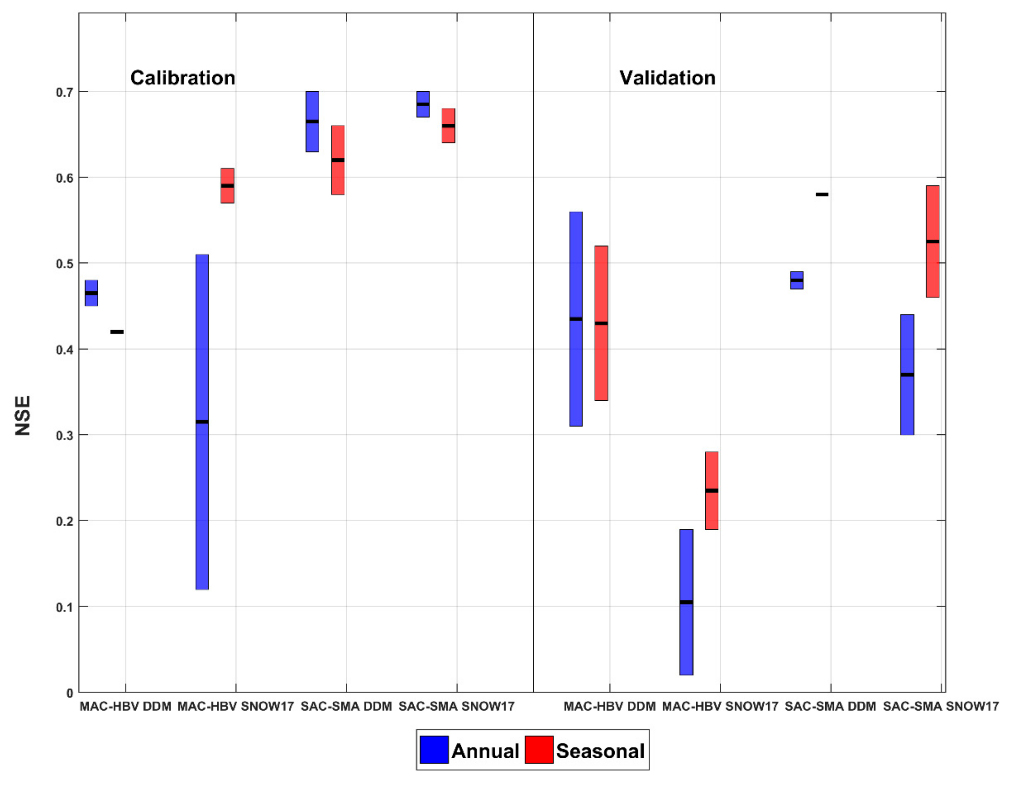
Spring peak flow statistics, shown in Table 2 and Table 3, at LGRB suggests that annual and seasonal MAC-HBV-DDM, MAC-HBV-SNOW17, SAC-SMA-DDM, and SAC-SMA-SNOW17 perform equally well in capturing the peak flow as they have nearly similar model means. A similar trend is observed at UASR (PFC in Table 4 and Table 5). Furthermore, insights into the sub-basin scale PFC statistics (Table 6) reveal that DDM is better at estimating peak flows at more than half of the sub-basins in both study areas. Further, investigation of NSE criterion at LGRB revealed that model combinations with DDM were as accurate as combinations with the SNOW-17 model (Figure 5) with relatively small differences in their model medians. At UASR (Figure 6), the performance of annual and seasonal MAC-HBV and SAC-SMA models indicated a marked increase in the median of NSE when DDM is used compared to the SNOW-17 model during the validation period. Overall, a comparison of all statistics suggests that the performance of DDM was very competitive with the SNOW-17 model at LGRB while it outperformed the SNOW-17 model significantly at UASR.
4.2. Results of Annually and Seasonally Calibrated Models
Spring season performance of annual and seasonal models for LGRB is presented in Table 2 and Table 3 and Figure 5. As shown, the mean values (Tables) of NSE and KGE and median of NSEs (Figure 5) for all the model combinations exceed 0.5 suggesting reasonable agreement between computed and recorded reservoir inflow. Comparison of calibration approaches indicates that seasonal models have either similar or higher NSE values for all the model structures during the training period. During the testing period, seasonally calibrated MAC-HBV-DDM and MAC-HBV-SNOW-17 models have higher NSE values than their annually calibrated counterparts. For example, by using seasonal models, the median of NSEs increase by 11% and 5% compared to using annual MAC-HBV-DDM and MAC-HBV-SNOW17 models, respectively. The model performance of UASR in terms of NSE is presented in Table 4 and Table 5 and Figure 6. Annual model optimization improves the median of NSE for MAC-HBV-DDM, SAC-SMA-DDM, and SAC-SMA-SNOW17 models marginally when evaluated for the calibration period. However, the seasonal MAC-HBV-SNOW17 model provides a marked improvement in the median of NSE. In contrast, all the seasonal model combinations produce higher or identical NSE median values compared to annually optimized models for the testing period. To illustrate, the median of NSEs drastically increase by 56%, 17%, and 28% when the seasonal MAC-HBV-SNOW17, SAC-SMA-DDM, and SAC-SMA-SNOW17 models are used as compared to annual models for the validation period, respectively. In summary, comparative results suggest that out of 16 total model scenarios for the entire duration at both the study sites, 12 model scenarios produce relatively higher or equal NSE medians when seasonally optimized models are used as compared to the annually optimized models.
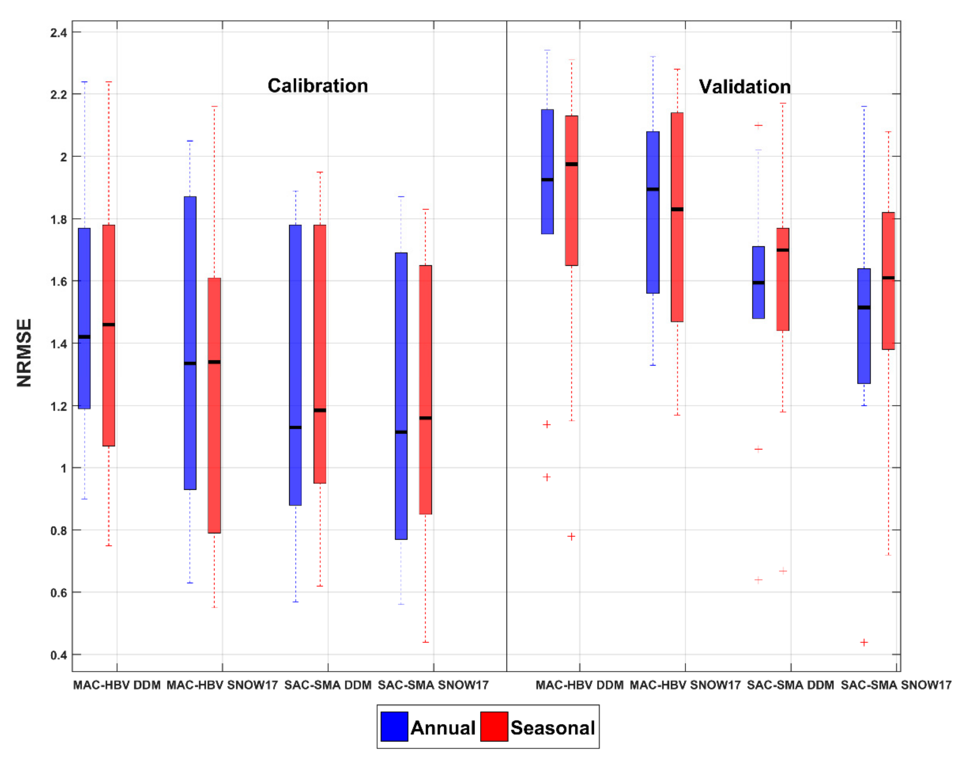
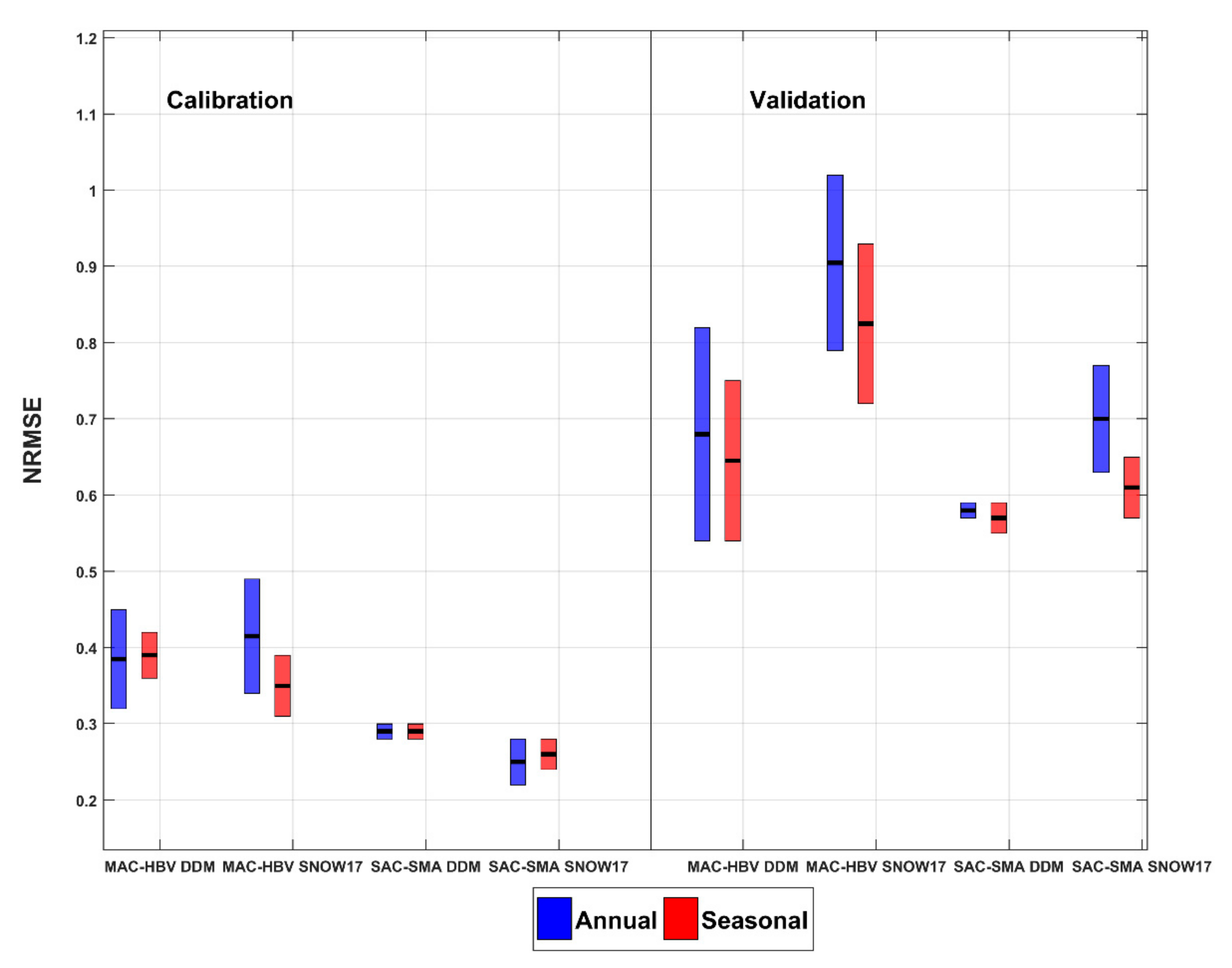
Figure 7 and the NRMSE in Table 2 and Table 3 show the spring peak flow performance at LGRB. Annual models perform better since a marginal reduction in the median of NRMSE is obtained for the calibration and validation periods for all the model structures (Figure 7). The Wilcoxon rank sum test for equality of medians (α = 0.05) was performed to determine the statistical significance between the medians of annually and seasonally calibrated models and it found no difference in the medians of NRMSE. Interestingly, for calibration and validation periods, Table 2 and Table 3 indicate that seasonal models are as accurate as annual models in predicting the peak flows for all the model structures. Confirming with the above results, more than half of the sub-basins show a reduction in NRMSE with seasonal models than annual models at LGRB (Table 6). For the second study site-UASR, NRMSE statistics are presented in Figure 8. It clearly indicates that the median of NRMSE for all seasonally calibrated models show better or comparable performance to annually calibrated models. For example, the median of NRMSE is reduced by 16% and 9% when seasonal MAC-HBV-SNOW17 and SAC-SMA-SNOW-17 models are used as compared to their annual model counterparts during the validation period. Overall, seasonally optimized models provide competitive or better performance for the majority of sub-basins (Table 6) as compared to annually calibrated models at both the watersheds.
4.3. Comparison between Hydrological Models: MAC-HBV and SAC-SMA
Performance of the MAC-HBV and SAC-SMA hydrological models for the spring season is shown in Figure 5 and Table 2 and Table 3. Figure 5 suggests that SAC-SMA model combinations perform better than MAC-HBV model combinations during the calibration period at LGRB. For instance, annual and seasonal SAC-SMA-DDM and SAC-SMA-SNOW17 models indicate an increase in the median of NSE by 43%, 54%, 47%, and 11% compared to the equivalent MAC-HBV model combinations during the calibration period, respectively. A similar trend was observed in the validation period, but it revealed a large increase in the median of NSEs when SAC-SMA model combinations were used. For example, the median of NSE increased by 270% and 126% with annual and seasonal SAC-SMA-SNOW17 models as compared to annual and seasonal MAC-HBV-SNOW17 models, respectively. At UASR, NSE (Figure 6) and KGE (Table 4 and Table 5) statistics suggest that most SAC-SMA model combinations outperformed MAC-HBV model combinations during both the calibration and validation periods.
NRMSE metrics provide an accurate measure of peak flow model performance and are provided in Figure 7; Figure 8 in Table 2, Table 3, Table 4 and Table 5 for both study areas. The median NRMSE at LGRB (Figure 7) ranges from 1.83 to 1.97 mm/day for MAC-HBV model combinations, whereas for SAC-SMA model combinations it ranges from 1.51 to 1.70 mm/day for the validation periods. At UASR (Figure 8), the median NRMSE is lower for the SAC-SMA model combinations during both the calibration and validation periods. To illustrate, the median NRMSE is decreased by 14%, 12%, 6%, and 26% when annual and seasonal SAC-SMA-DDM and SAC-SMA-SNOW17 models are used instead of their respective MAC-HBV model combinations during the validation period. Overall, whatever optimization approach or snowmelt routine is used, SAC-SMA model combinations outperformed the MAC-HBV model combinations in estimating spring season flows and spring peak flows at both study sites.
4.4. Visual Inspection of Model Performance
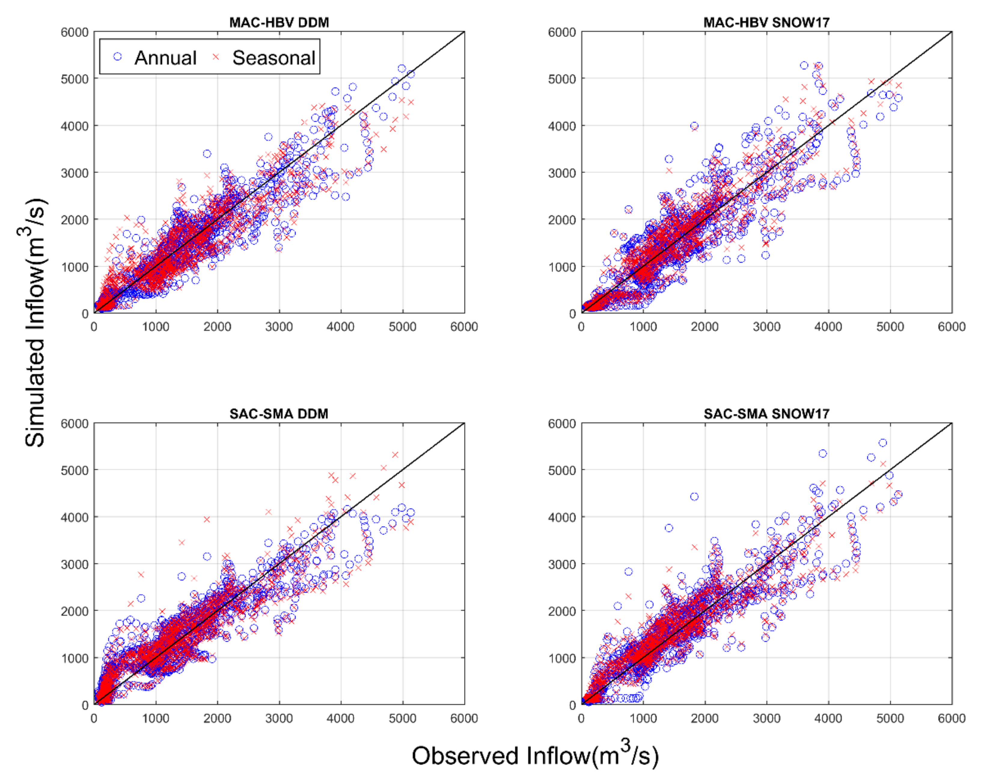
To further assess the general model performance, scatterplots of observed and simulated reservoir inflow are presented for the model combinations at LGRB (Figure 9). As mentioned earlier, model assessment is solely based on the spring season (Apr–Jun) performance. Figure 9 clearly illustrates that scatterplots for SAC-SMA-DDM model fall near the ideal or 45° line compared to all other model combinations. While annual models tend to underestimate the inflows above 3000 cms consistently, seasonal models show less dispersion and better capture inflows.
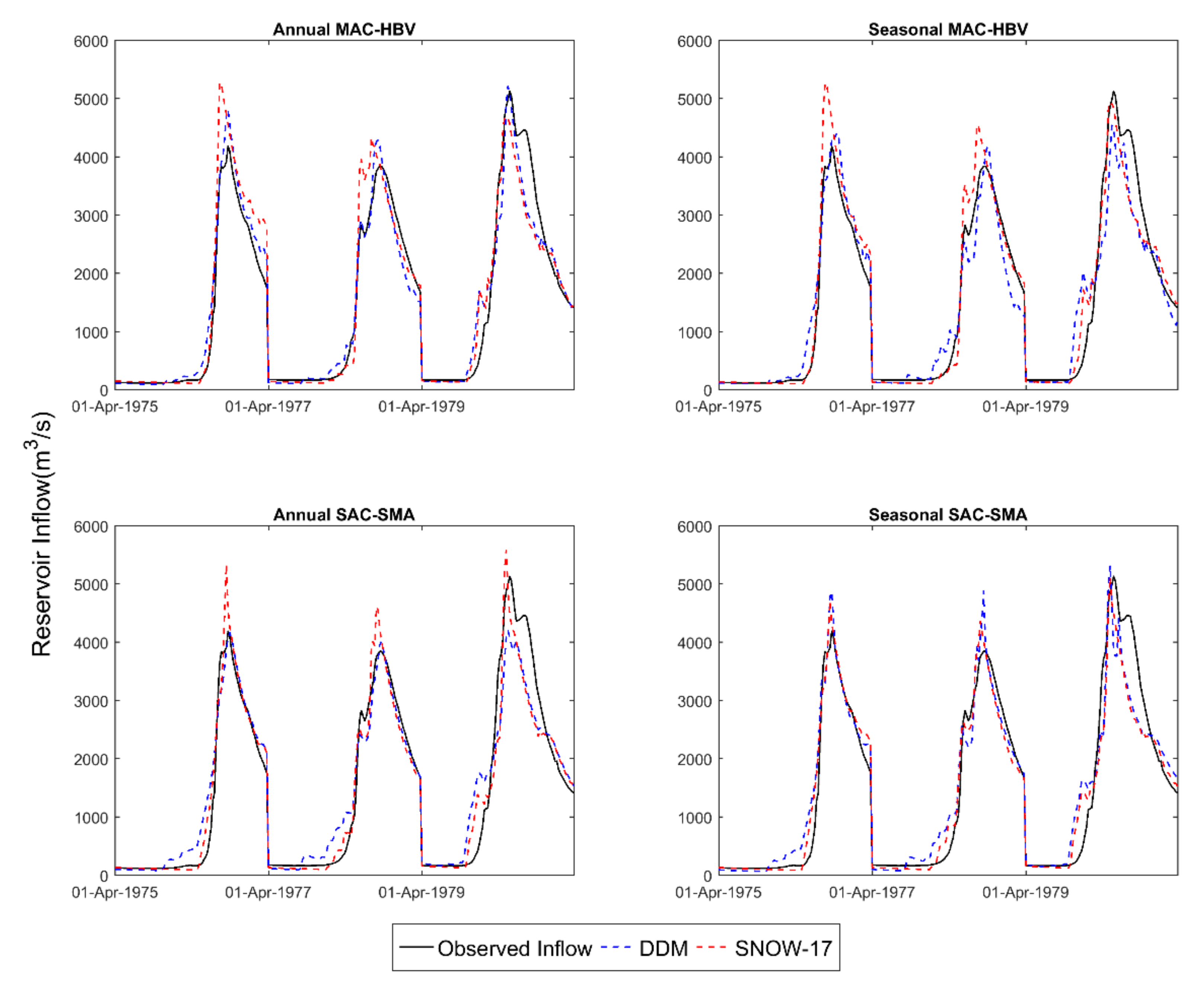
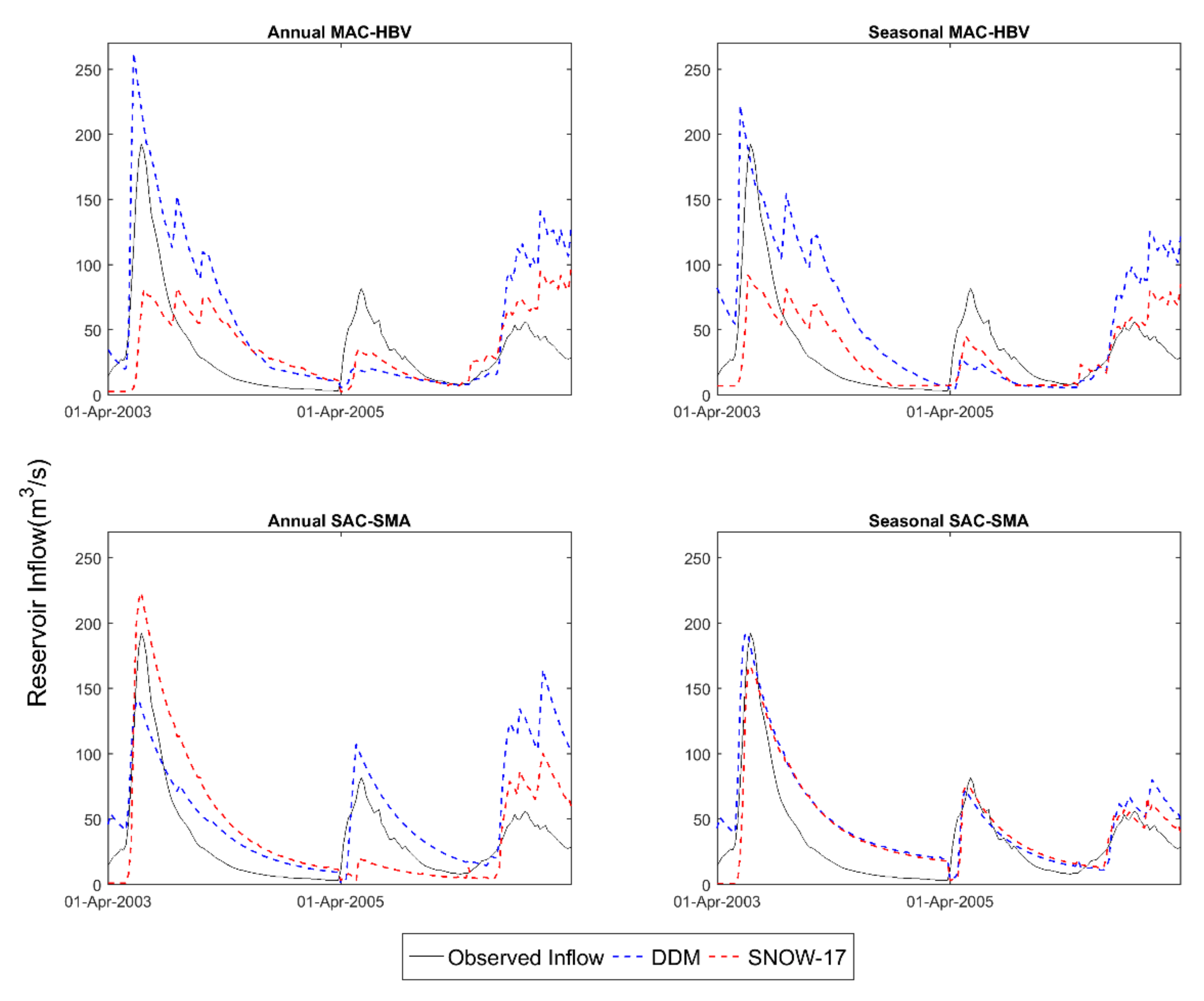
In order to further substantiate the model performance statistics and scatterplots discussed above, hydrographs of recorded and computed reservoir inflows are presented in Figure 10 and Figure 11 for LGRB and UASR, respectively. For LGRB (Figure 10), the seasonally calibrated SAC-SMA model appears more effective at simulating the magnitude and timing of the spring season inflow than annual MAC-HBV, annual SAC-SMA, and seasonal MAC-HBV models. It also indicates that DDM can estimate peak flows as accurately as the SNOW-17 model. Additionally, at UASR (Figure 11), plots clearly reveal that the seasonally calibrated SAC-SMA model with DDM better captures observed peak flows and the shape of the hydrograph. Other model combinations tend to either under- or over-estimate and are unable to capture the rising and falling limb of the hydrograph. Thus, the overall examination of the figures for both study areas agrees with previously obtained model performance statistics, which indicate that the seasonal SAC-SMA model with DDM provides improved peak flow simulations.
5. Discussion
Snowmelt estimation is an important component of hydrologic modeling systems, especially for spring peak flow prediction in snow-dominated watersheds. Most operational forecast applications use temperature index-based approaches instead of energy budget models owing to a lack of continuous historical radiation observations. Therefore, this study used the DDM and the SNOW-17 model as they rely solely on temperature and precipitation for snowmelt estimation. The reservoir inflow estimates obtained from DDM were compared to those produced by the SNOW-17 model. Interestingly, the results showed that DDM has a high ability to capture snowmelt driven spring floods and was found to be comparable to or better than the SNOW-17 model. This study showed the flexibility of DDM in adapting to different hydrologic models and hydrological systems (Figure 10 and Figure 11) and providing consistently good results. Better performance of DDM may be attributed to forested and undeveloped sites used in the study where DDM has well demonstrated its ability to capture snowmelt induced peaks [21,52,53]. The successful application of snowmelt estimation methods at LGRB may be due to the temperature being a better indicator of surface energy balance in forested areas as canopy diminishes the effects of direct solar radiation and wind [44,54]. Whereas, the dominant land cover in UASR is cropland [55], so temperature may not be sufficient in explaining the physical basis of involved snow processes leading to a relatively limited performance at UASR. SNOW-17 model has been used operationally for the past few decades; however, it was found to be less effective in achieving accurate spring flow prediction particularly at UASR (Figure 10). This outcome may be due to the watershed not being spatially discretized or divided into elevation zones [38]. However, this finding is consistent with Lundquist and Flint [56] where limited performance of the SNOW-17 model was demonstrated in topographically complex terrain.
Parameter optimization is an important part of the hydrologic modeling process. In the case of extreme events, operational hydrologists require a calibration approach that is computationally efficient [3] and has a high ability to capture the hydrological information driven by historical input data. As optimizing model parameters considering annual time series is inefficient, particularly when seasonal forecasts are of interest, we evaluated the seasonal model calibration approach to test its robustness against annually calibrated models in capturing the spring season reservoir inflow. Results suggested that seasonal models performed competitively and often better than an annual model calibration approach at LGRB and UARB (Figure 6 and Figure 7). The results of the work presented here are in agreement with a similar study by Paik et al. [57], where a comparative analysis to study seasonal and non-seasonal model calibration was performed, and the results revealed that seasonal models clearly outperformed the non-seasonal models. A possible limitation of the annual calibration approach can be that it accounts for the low, medium, and high flows simultaneously where most of the year-round flows are low and medium flows except the spring season flow [58]. Thus, due to high variability in the annual flow regimes, optimal model parameter estimates obtained by calibrating annually may not be very sensitive to the spring peak flows [57]. Unlike annual models, seasonal models have an advantage of being calibrated specifically to the spring season flows and thus demonstrated a higher ability to capture the recorded high flows.
MAC-HBV and SAC-SMA hydrologic models were used in the study for inflow forecasting. SAC-SMA model combinations demonstrated the capability of simulating the spring peak flows consistently better than the MAC-HBV model. In the hydrologic system of UASR, MAC-HBV model performance is relatively poor compared to LGRB. Spring snowmelt flows at UASR are highly affected by the release of infiltrated snowmelt water from the frozen soils as basin exhibits frozen ground effect [55]. Considering such conditions, it is essential to determine complicated soil moisture dynamics appropriately. However, the MAC-HBV model accounts for soil moisture changes only in a simplified form [32]. Such simplifications are presumed the likely cause for the poor performance of the MAC-HBV model. Moreover, limited performance can be partially attributed to the hydrological complexity emerging out of the fill and spill of potholes in the UASR [29,55,59]. Nevertheless, more accurate estimates of flow are obtained here using conceptual models than the results obtained by Unduche et al. [55] where four hydrological models specifically developed for Shellmouth Reservoir inflow forecasts were evaluated for operational flood forecasting at UASR. Their results demonstrated poor performance when the HSPF and HBV-EC conceptual models were assessed for the spring season. Awol et al. [60] performed a comparative analysis of lumped conceptual models (SAC-SMA and MAC-HBV), a distributed WATFLOOD model, and a macroscale land surface model (VIC) for short- and medium-range flood forecasting at UASR. Their results also suggested that SAC-SMA provided better performance than other models investigated at the study site.
6. Conclusions
A comparative analysis was performed to assess the effectiveness and accuracy of the degree-day method (DDM) as compared to more complex SNOW-17 model, focusing on the spring season peak flow and reservoir inflow simulations. Additionally, the performance of seasonal and annual calibration approaches for both the MAC-HBV and SAC-SMA hydrological models for accurate spring peak flow prediction was evaluated. The study was conducted on the La-Grande River Basin (LGRB, Quebec, Canada), and on the Upper Assiniboine River at Shellmouth Reservoir (UASR, Manitoba, Canada). This study led to the evaluation of eight model scenarios for each watershed.
Analyses of the results indicate that DDM performed consistently better than or comparable to SNOW-17 at both the watersheds. Moreover, the flexibility and applicability of DDM was well demonstrated on the more complex terrain of the UASR, where the SNOW-17 model was unable to capture the spring flood accurately. The comparison of seasonal models with annual models suggested that calibrating over spring season offers an effective alternative to improve spring peak flow prediction. Seasonal model calibration performed as well or better than annual model calibration. Further, SAC-SMA hydrologic model was shown to outperform MAC-HBV model for both snowmelt estimation techniques, both calibration approaches, and in both study areas. Overall, improved spring peak flow results are obtained by using DDM with the seasonally calibrated SAC-SMA model. Furthermore, the added advantage of using DDM is that it is simple and easy to implement, and the use of seasonally calibrated models has a lower computational cost – hence it offers a cost-effective solution. The study results will further aid flood forecasters in selecting an effective combination of methods for operational applications in snow-dominated watersheds.
Author Contributions
Conceptualization, J.A. and P.C.; methodology, J.A. and P.C.; software, J.A. and P.C.; validation, J.A. and P.C.; formal analysis, J.A.; investigation, J.A.; data curation, J.A.; visualization, P.C.; writing—original draft preparation, J.A.; writing—review and editing, P.C.; supervision, P.C.; funding acquisition, P.C. All authors have read and agreed to the published version of the manuscript.
Funding
This work was supported by the Natural Sciences and Engineering Research Council of Canada (NSERC) under Canadian FloodNet Project (Grant number: NETGP 451456).
Acknowledgments
The authors appreciate the help and constructive suggestions provided by Dr. Tara Razavi. Thanks to Hydro-Québec and Manitoba Infrastructure for providing the study data and information. The authors are grateful to Dr James Leach for editing the manuscript.
Conflicts of Interest
The authors declare no conflict of interest.
References
- Ahmed, S.; Coulibaly, P.; Tsanis, I. Improved spring peak-flow forecasting using ensemble meteorological predictions. J. Hydrol. Eng. 2015, 20, 04014044. [Google Scholar] [CrossRef]
- Coulibaly, P. Impact of meteorological predictions on real-time spring flow forecasting. Hydrol. Process. 2003, 17, 3791–3801. [Google Scholar] [CrossRef]
- Awol, F.S.; Coulibaly, P.; Tolson, B.A. Event-based model calibration approaches for selecting representative distributed parameters in semi-urban watersheds. Adv. Water Resour. 2018, 118, 12–27. [Google Scholar] [CrossRef]
- Krauße, T.; Cullmann, J.; Saile, P.; Schmitz, G.H. Hydrology and Earth System Sciences Robust multi-objective calibration strategies-possibilities for improving flood forecasting. Hydrol. Earth Syst. Sci. 2012, 16, 3579–3606. [Google Scholar] [CrossRef] [Green Version]
- Etchevers, P.; Martin, E.; Brown, R.; Fierz, C.; Lejeune, Y.; Bazile, E.; Boone, A.; Dai, Y.-J.; Essery, R.; Fernandez, A.; et al. Validation of the Energy Budget of an Alpine Snowpack Simulated by Several Snow Models (SnowMIP project). Ann. Glaciol. 2004, 38, 150–158. [Google Scholar] [CrossRef] [Green Version]
- Mahanama, S.; Livneh, B.; Koster, R.; Lettenmaier, D.; Reichle, R. Soil Moisture, Snow, and Seasonal Streamflow Forecasts in the United States. J. Hydrometeorol. 2012, 13, 189–203. [Google Scholar] [CrossRef]
- Troin, M.; Arsenault, R.; Brissette, F. Performance and Uncertainty Evaluation of Snow Models on Snowmelt Flow Simulations over a Nordic Catchment (Mistassibi, Canada). Hydrology 2015, 2, 289–317. [Google Scholar] [CrossRef] [Green Version]
- Debele, B.; Srinivasan, R.; Gosain, A.K. Comparison of Process-Based and Temperature-Index Snowmelt Modeling in SWAT Conflict Resolution and Equitable Apportionment in Transboundary Basins View project Hydrological modeling View project Comparison of Process-Based and Temperature-Index Snowmelt. Water Resour. Manag. 2010, 24, 1065–1088. [Google Scholar] [CrossRef]
- Rango, A.; Martinec, J. Revisiting the degree-day method for snowmelt computations. J. Am. Water Resour. Assoc. 1995, 31, 657–669. [Google Scholar] [CrossRef]
- Pomeroy, J.W.; De Boer, D.; Martz, L.W. Hydrology and Water Resources of Saskatchewan, Centre for Hydrology; University of Saskatchewan: Saskatoon, SK, Canada, 2005. [Google Scholar]
- Essery, R.; Rutter, N.; Pomeroy, J.; Baxter, R.; Stahli, M.; Gustafsson, D.; Barr, A.; Bartlett, P.; Elder, K. An Evaluation of Forest Snow Process Simulations. Bull. Am. Meteorol. Soc. 2009, 90, 1120–1135. [Google Scholar] [CrossRef] [Green Version]
- Valeo, C.; Ho, C.L.I. Modelling urban snowmelt runoff. J. Hydrol. 2004, 299, 237–251. [Google Scholar] [CrossRef]
- Raleigh, M.S.; Lundquist, J.D. Comparing and combining SWE estimates from the SNOW-17 model using PRISM and SWE reconstruction. Water Resour. Res. 2012, 48. [Google Scholar] [CrossRef] [Green Version]
- Bokhorst, S.; Pedersen, S.H.; Brucker, L.; Anisimov, O.; Bjerke, J.W.; Brown, R.D.; Ehrich, D.; Essery, R.L.H.; Heilig, A.; Ingvander, S.; et al. Changing Arctic snow cover: A review of recent developments and assessment of future needs for observations, modelling, and impacts. Ambio 2016, 45, 516–537. [Google Scholar] [CrossRef] [PubMed] [Green Version]
- Moghadas, S.; Gustafsson, A.M.; Muthanna, T.M.; Marsalek, J.; Viklander, M. Review of models and procedures for modelling urban snowmelt. Urban Water J. 2016, 13, 396–411. [Google Scholar] [CrossRef]
- Essery, R.; Morin, S.; Lejeune, Y.; Ménard, C.B. A comparison of 1701 snow models using observations from an alpine site. Adv. Water Resour. 2013, 55, 131–148. [Google Scholar] [CrossRef] [Green Version]
- Rutter, N.; Essery, R.; Pomeroy, J.; Altimir, N.; Andreadis, K.; Baker, I.; Barr, A.; Bartlett, P.; Boone, A.; Deng, H.; et al. Evaluation of forest snow processes models (SnowMIP2). J. Geophys. Res. Atmos. 2009, 114. [Google Scholar] [CrossRef] [Green Version]
- Bowling, L.; Lettenmaier, D.; Nijssen, B. Simulation of high-latitude hydrological processes in the Torne–Kalix basin: PILPS Phase 2 (e): 1: Experiment description and summary intercomparisons. Glob. Planet. Chang. 2003, 38, 1–30. [Google Scholar] [CrossRef] [Green Version]
- Raleigh, M.S.; Livneh, B.; Lapo, K.; Lundquist, J.D. How does availability of meteorological forcing data impact physically based snowpack simulations? J. Hydrometeorol. 2016, 17, 99–120. [Google Scholar] [CrossRef]
- Förster, K.; Meon, G.; Marke, T.; Strasser, U. Effect of meteorological forcing and snow model complexity on hydrological simulations in the Sieber catchment (Harz Mountains, Germany). Hydrol. Earth Syst. Sci. 2014, 18, 4703–4720. [Google Scholar] [CrossRef] [Green Version]
- World Meteorological Organization. Intercomparison of Models of Snowmelt Runoff; Operational Hydrology Report No. 23; WMO No: 646; WMO: Geneva, Switzerland, 1986. [Google Scholar]
- Hock, R. Temperature index melt modelling in mountain areas. J. Hydrol. 2003, 282, 104–115. [Google Scholar] [CrossRef]
- Kustas, W.P.; Rango, A.; Uijlenhoet, R. A simple energy budget algorithm for the snowmelt runoff model. Water Resour. Res. 1994, 30, 1515–1527. [Google Scholar] [CrossRef]
- Nijssen, B.; Bowling, L.; Lettenmaier, D. Simulation of high latitude hydrological processes in the Torne–Kalix basin: PILPS Phase 2 (e): 2: Comparison of model results with observations. Glob. Planet. Chang. 2003, 38, 31–53. [Google Scholar] [CrossRef] [Green Version]
- Franz, K.J.; Butcher, P.; Ajami, N.K. Addressing snow model uncertainty for hydrologic prediction. Adv. Water Resour. 2010, 33, 820–832. [Google Scholar] [CrossRef]
- Kumar, M.; Marks, D.; Dozier, J.; Reba, M.; Winstral, A. Evaluation of distributed hydrologic impacts of temperature-index and energy-based snow models. Adv. Water Resour. 2013, 56, 77–89. [Google Scholar] [CrossRef]
- Hernández-Henríquez, M.A.; Mlynowski, T.J.; Déry, S.J. Reconstructing the natural streamflow of a regulated river: A case study of la grande rivière, Québec, Canada. Can. Water Resour. J. 2010, 35, 301–316. [Google Scholar] [CrossRef] [Green Version]
- Coulibaly, P.; Keum, J. Snow Network Design and Evaluation for La Grande River Basin; Technical Report to Hydro-Quebec; McMaster University: Hamilton, ON, Canada, 2016. [Google Scholar]
- Blais, E.L.; Greshuk, J.; Stadnyk, T. The 2011 flood event in the Assiniboine River Basin: Causes, assessment and damages. Can. Water Resour. J. 2016, 41, 74–84. [Google Scholar] [CrossRef]
- Fang, X.; Minke, A.; Pomeroy, J.; Brown, T.; Westbrook, C.; Guo, X.; Guangul, S. A Review of Canadian Prairie Hydrology: Principles, Modelling and Response to Land Use and Drainage Change; Centre for Hydrology Report #2, Version 2; University of Saskatchewan: Saskatoon, SK, Canada, 2007. [Google Scholar]
- Shrestha, R.R.; Dibike, Y.B.; Prowse, T.D. Modeling Climate Change Impacts on Hydrology and Nutrient Loading in the Upper Assiniboine Catchment1. JAWRA J. Am. Water Resour. Assoc. 2012, 48, 74–89. [Google Scholar] [CrossRef]
- Samuel, J.; Coulibaly, P.; Metcalfe, R.A. Estimation of continuous streamflow in ontario ungauged basins: Comparison of regionalization methods. J. Hydrol. Eng. 2011, 16, 447–459. [Google Scholar] [CrossRef]
- Bergström, S. Development and Application of a Conceptual Runoff Model for Scandinavian Catchments; Technical Report No. RHO7; Swedish Meteorological and Hydrological Institute: Norrköping, Sweden, 1976. [Google Scholar]
- Razavi, T.; Coulibaly, P. Improving streamflow estimation in ungauged basins using a multi-modelling approach. Hydrol. Sci. J. 2016, 61, 2668–2679. [Google Scholar] [CrossRef] [Green Version]
- Samuel, J.; Coulibaly, P.; Metcalfe, R.A. Identification of rainfall-runoff model for improved baseflow estimation in ungauged basins. Hydrol. Process. 2012, 26, 356–366. [Google Scholar] [CrossRef]
- Sharma, M.; Coulibaly, P.; Dibike, Y. Assessing the need for downscaling RCM data for hydrologic impact study. J. Hydrol. Eng. 2011, 16, 534–539. [Google Scholar] [CrossRef]
- Vrugt, J.A.; Gupta, H.V.; Nualláin, B.; Bouten, W. Real-Time Data Assimilation for Operational Ensemble Streamflow Forecasting. J. Hydrometeorol. 2006, 7, 548–565. [Google Scholar] [CrossRef]
- Anderson, E. Snow Accumulation and Ablation Model–SNOW-17; US National Weather Service: Silver Spring, MD, USA, 2006.
- He, M.; Hogue, T.S.; Franz, K.J.; Margulis, S.A.; Vrugt, J.A. Corruption of parameter behavior and regionalization by model and forcing data errors: A Bayesian example using the SNOW17 model. Water Resour. Res. 2011, 47. [Google Scholar] [CrossRef]
- Anderson, E. National Weather Service River Forecast System: Snow Accumulation and Ablation Model; NOAA Tech. Memo., NWS Hydro-17; National Weather Service (NWS): Silver Spring, MD, USA, 1973.
- Burnash, R.; Ferral, R.; McGuire, R. A Generalized Streamflow Simulation System: Conceptual Modeling for Digital Computers; Dept. of Water Resources, State of California: Sacramento, CA, USA, 1973.
- Reed, S.; Koren, V.; Smith, M.; Zhang, Z.; Moreda, F.; Seo, D.J. Overall distributed model intercomparison project results. J. Hydrol. 2004, 298, 27–60. [Google Scholar] [CrossRef]
- Day, G.N. Extended streamflow forecasting using NWSRFS. J. Water Resour. Plan. Manag. 1985, 111, 157–170. [Google Scholar] [CrossRef]
- Ohmura, A. Physical Basis for the Temperature-Based Melt-Index Method. J. Appl. Meteorol. 2001, 40, 753–761. [Google Scholar] [CrossRef]
- Hogue, T.S.; Gupta, H.; Sorooshian, S. A “User-Friendly” approach to parameter estimation in hydrologic models. J. Hydrol. 2006, 320, 202–217. [Google Scholar] [CrossRef]
- Tang, Y. Advancing Hydrologic Model Evaluation and Identification Using Multiobejctive Calibration, Sensitivity Analysis and Parallel Computation. Ph.D. Thesis, The Graduate School, The Pennsylvania State University, State College, PA, USA, 2007. [Google Scholar]
- Kratzert, F.; Klotz, D.; Brenner, C.; Schulz, K.; Herrnegger, M. Rainfall-runoff modelling using Long Short-Term Memory (LSTM) networks. Hydrol. Earth Syst. Sci. 2018, 22, 6005–6022. [Google Scholar] [CrossRef] [Green Version]
- Eberhart, R.; Kennedy, J. A New Optimizer Using Particle Swarm Theory. In Proceedings of the Sixth International Symposium on Micro Machine and Human Science, Nagoya, Japan, 4–6 October 1995. [Google Scholar]
- Razavi, T.; Coulibaly, P. An evaluation of regionalization and watershed classification schemes for continuous daily streamflow prediction in ungauged watersheds. Can. Water Resour. J. 2017, 42, 2–20. [Google Scholar] [CrossRef]
- Gupta, H.V.; Kling, H.; Yilmaz, K.K.; Martinez, G.F. Decomposition of the mean squared error and NSE performance criteria: Implications for improving hydrological modelling. J. Hydrol. 2009, 377, 80–91. [Google Scholar] [CrossRef] [Green Version]
- Coulibaly, P.; Anctil, F.; Bobée, B. Multivariate reservoir inflow forecasting using temporal neural networks. J. Hydrol. Eng. 2001, 6, 367–376. [Google Scholar] [CrossRef]
- Singh, P.; Jain, S.K. Modelling of streamflow and its components for a large Himalayan basin with predominant snowmelt yields. Hydrol. Sci. J. 2003, 48, 257–276. [Google Scholar] [CrossRef]
- Réveillet, M.; Six, D.; Vincent, C.; Rabatel, A.; Dumont, M.; Lafaysse, M.; Morin, S.; Vionnet, V.; Litt, M. Relative performance of empirical and physical models in assessing the seasonal and annual glacier surface mass balance of Saint-Sorlin Glacier (French Alps). Cryosphere 2018, 12, 1367–1386. [Google Scholar] [CrossRef] [Green Version]
- Melloh, R.A. A Synopsis and Comparison of Selected Snowmelt Algorithms; CRREL Report 99-8; US Army Corps of Engineers: Hanover, NH, USA, 1999.
- Unduche, F.; Tolossa, H.; Senbeta, D.; Zhu, E. Evaluation of four hydrological models for operational flood forecasting in a Canadian Prairie watershed. Hydrol. Sci. J. 2018, 63, 1133–1149. [Google Scholar] [CrossRef] [Green Version]
- Lundquist, J.D.; Flint, A.L. Onset of snowmelt and streamflow in 2004 in the Western Unites States: How shading may affect spring streamflow timing in a warmer world. J. Hydrometeorol. 2006, 7, 1199–1217. [Google Scholar] [CrossRef] [Green Version]
- Paik, K.; Kim, J.H.; Kim, H.S.; Lee, D.R. A conceptual rainfall-runoff model considering seasonal variation. Hydrol. Process. 2005, 19, 3837–3850. [Google Scholar] [CrossRef]
- Kim, H.S.; Lee, S. Assessment of a seasonal calibration technique using multiple objectives in rainfall-runoff analysis. Hydrol. Process. 2014, 28, 2159–2173. [Google Scholar] [CrossRef]
- Muhammad, A.; Stadnyk, T.; Unduche, F.; Coulibaly, P. Multi-Model Approaches for Improving Seasonal Ensemble Streamflow Prediction Scheme with Various Statistical Post-Processing Techniques in the Canadian Prairie Region. Water 2018, 10, 1604. [Google Scholar] [CrossRef] [Green Version]
- Awol, F.S.; Coulibaly, P.; Tsanis, I.; Unduche, F. Identification of hydrological models for enhanced ensemble reservoir inflow forecasting in a large complex prairiewatershed. Water 2019, 11, 2201. [Google Scholar] [CrossRef] [Green Version]
Figure 1.
(a) La-Grande River Basin (LGRB), Quebec, Canada (Left) and (b) Upper Assiniboine River at Shellmouth Reservoir (UASR), Manitoba, Canada (Right).
Figure 1.
(a) La-Grande River Basin (LGRB), Quebec, Canada (Left) and (b) Upper Assiniboine River at Shellmouth Reservoir (UASR), Manitoba, Canada (Right).

Figure 2.
Model Set-up.

Figure 3.
Model Improvement (defined by % reduction in RMSE) obtained by using the SNOW-17 model instead of DDM for LGRB. Positive values mean model improvement when coupled with the SNOW-17 model, while negative values mean model deterioration due to implementation of the SNOW-17 model (with DDM taken as a base model for evaluation). Boxes are delimited by the 25th and 75th percentiles, the median value is printed in the boxes, and the whiskers are delimited by 10th and 90th percentiles.

Figure 4.
Model Improvement (defined by % reduction in RMSE) obtained by using the SNOW-17 model than DDM for UASR. The description is the same as in Figure 3, and as the model was calibrated at two stations, boxes here represent statistics for both the locations considered.
Figure 4.
Model Improvement (defined by % reduction in RMSE) obtained by using the SNOW-17 model than DDM for UASR. The description is the same as in Figure 3, and as the model was calibrated at two stations, boxes here represent statistics for both the locations considered.

Figure 5.
NSE statistics for MAC-HBV-DDM, MAC-HBV-SNOW-17, SAC-SMA-DDM, SAC-SMA-SNOW-17 model structures for annual and seasonal models of LGRB. Boxplot description same as Figure 3, except the median is marked with a thick black line inside boxes.
Figure 5.
NSE statistics for MAC-HBV-DDM, MAC-HBV-SNOW-17, SAC-SMA-DDM, SAC-SMA-SNOW-17 model structures for annual and seasonal models of LGRB. Boxplot description same as Figure 3, except the median is marked with a thick black line inside boxes.

Figure 6.
NSE statistics for MAC-HBV-DDM, MAC-HBV-SNOW-17, SAC-SMA-DDM, SAC-SMA-SNOW-17 model structures for annual and seasonal models of UASR. See Figure 4 for a description of the boxplots, and the median is marked with a thick black line inside boxes.
Figure 6.
NSE statistics for MAC-HBV-DDM, MAC-HBV-SNOW-17, SAC-SMA-DDM, SAC-SMA-SNOW-17 model structures for annual and seasonal models of UASR. See Figure 4 for a description of the boxplots, and the median is marked with a thick black line inside boxes.

Figure 7.
NRMSE statistics for MAC-HBV-DDM, MAC-HBV-SNOW-17, SAC-SMA-DDM, SAC-SMA-SNOW-17 model combinations for annual and seasonal models of LGRB. NRMSE is computed for spring season flows above 75 percentile. See Figure 5 for box plot description.
Figure 7.
NRMSE statistics for MAC-HBV-DDM, MAC-HBV-SNOW-17, SAC-SMA-DDM, SAC-SMA-SNOW-17 model combinations for annual and seasonal models of LGRB. NRMSE is computed for spring season flows above 75 percentile. See Figure 5 for box plot description.

Figure 8.
NRMSE statistics for MAC-HBV-DDM, MAC-HBV-SNOW-17, SAC-SMA-DDM, SAC-SMA-SNOW-17 model combinations for annual and seasonal models of UASR. See Figure 6 for box plot description.
Figure 8.
NRMSE statistics for MAC-HBV-DDM, MAC-HBV-SNOW-17, SAC-SMA-DDM, SAC-SMA-SNOW-17 model combinations for annual and seasonal models of UASR. See Figure 6 for box plot description.

Figure 9.
Validation scatterplots for the spring season at LGRB.

Figure 10.
Validation hydrographs for spring season inflow simulations for LGRB.

Figure 11.
Validation hydrographs showing spring season inflow simulations for UASR.


| Parameter Code | Description | Unit | Ranges |
|---|---|---|---|
| SAC-SMA | |||
| UZTWM | Upper-zone tension water maximum storage | mm | 1–150 |
| UZFWM | Upper-zone free water maximum storage | mm | 1–150 |
| UZK | Upper-zone free water lateral depletion rate | day−1 | 0.1–0.5 |
| PCTIM | Impervious fraction of the watershed area | - | 0–0.1 |
| ADIMP | Additional impervious area | - | 0–0.4 |
| ZPERC | Maximum percolation rate | - | 1–250 |
| REXP | Exponent of the percolation equation | - | 1–5 |
| LZTWM | Lower-zone tension water maximum storage | mm | 1–500 |
| LZFSM | Lower-zone free water supplemental maximum storage | mm | 1–1000 |
| LZFPM | Lower-zone free water primary maximum storage | mm | 1–1000 |
| LZSK | Lower-zone supplemental free water lateral depletion rate | day−1 | 0.01–0.25 |
| LZPK | Lower-zone primary free water lateral depletion rate | day−1 | 0.0001–0.025 |
| PFREE | Fraction percolating from upper to lower zone free water storage | - | 0–0.6 |
| Rq | Routing coefficient | - | 0.5–1.5 |
| MAC-HBV | |||
| athorn | Constant for Thornthwaite’s equation | - | 0.1–0.3 |
| fc | Maximum soil box water content | mm | 50–800 |
| lp | Limit for potential evaporation | mm/mm | 0.1*fc–0.9*fc |
| beta | Non-linear parameter controlling runoff generation | - | 0–10 |
| k0 | Flow recession coefficient in an upper soil reservoir | days | 1–30 |
| lsuz | A threshold value used to control response routing on an upper soil reservoir | mm | 1–100 |
| k1 | Flow recession coefficient in an upper soil reservoir | days | 30–100 |
| cperc | A constant percolation rate parameter | mm/day | 0.01–6 |
| k2 | Flow recession coefficient in a lower soil reservoir | days | 100–500 |
| alpha1 | An exponent in relation between outflow and storage representing non-linearity of storage – discharge relationship of lower reservoir | - | 0.5–1.25 |
| maxbas | A triangle weighting function for modelling a channel routing routine | days | 1–20 |
| DDM | |||
| tr | Upper threshold temperature to distinguish between rainfall and snowfall | °C | 0–2.5 |
| scf | Snowfall correction factor | - | 0.4–1.6 |
| ddf | Degree day factor | mm/day°C | 0–5.0 |
| rcr | Rainfall correction factor | - | 0.5–1.5 |
| SNOW17 | |||
| scf | Snowfall correction factor | - | 0.7–1.6 |
| uadj | Average wind function during rain-on-snow events | mm/mb/6 h | 0.03–0.19 |
| mbase | Base temperature for non-rain melt factor | °C | 0–1.0 |
| mfmax | Maximum melt factor considered to occur on Jun 21 | mm/6 h/°C | 0.5–2.0 |
| mfmin | Minimum melt factor considered to occur on Dec 21 | mm/6 h/°C | 0.05–0.49 |
| tipm | Antecedent snow temperature index | - | 0.01–1.0 |
| nmf | Maximum negative melt factor | mm/6 h/°C | 0.05–0.50 |
| plwhc | Percent liquid-water holding capacity | - | 0.02–0.3 |
| pxtemp1 | Lower limit temperature dividing transition from snow | °C | −2–0 |
| pxtemp2 | Upper limit temperature dividing rain from transition | °C | 1–3 |
Table 2.
Annual model performance statistics for LGRB.
| Model Calibration Mean | Model Validation Mean | |||||||||
|---|---|---|---|---|---|---|---|---|---|---|
| Models | NSE | KGE | NRMSE (mm/d) | PFC | Model Improvement (%) | NSE | KGE | NRMSE (mm/d) | PFC | Model Improvement (%) |
| MAC DDM | 0.76 | 0.83 | 1.49 | 0.40 | 1.13 | 0.56 | 0.68 | 1.83 | 0.46 | -4.21 |
| MAC SNOW-17 | 0.75 | 0.84 | 1.37 | 0.40 | 0.53 | 0.65 | 1.85 | 0.45 | ||
| SAC DDM | 0.82 | 0.87 | 1.24 | 0.35 | 0.83 | 0.66 | 0.72 | 1.54 | 0.42 | 4.27 |
| SAC SNOW-17 | 0.82 | 0.88 | 1.20 | 0.37 | 0.70 | 0.77 | 1.45 | 0.39 | ||
Table 3.
Seasonal model performance statistics for LGRB.
| Model Calibration Mean | Model Validation Mean | |||||||||
|---|---|---|---|---|---|---|---|---|---|---|
| Models | NSE | KGE | NRMSE (mm/d) | PFC | Model Improvement (%) | NSE | KGE | NRMSE (mm/d) | PFC | Model Improvement (%) |
| MAC DDM | 0.75 | 0.83 | 1.45 | 0.39 | 6.10 | 0.58 | 0.65 | 1.80 | 0.42 | 1.76 |
| MAC SNOW-17 | 0.78 | 0.85 | 1.28 | 0.35 | 0.55 | 0.66 | 1.78 | 0.45 | ||
| SAC DDM | 0.82 | 0.85 | 1.25 | 0.35 | 1.71 | 0.66 | 0.71 | 1.60 | 0.42 | 2.90 |
| SAC SNOW-17 | 0.82 | 0.87 | 1.19 | 0.32 | 0.66 | 0.75 | 1.54 | 0.43 | ||
Table 4.
Annual model performance statistics for UASR.
| Calibration | Validation | |||||||||
|---|---|---|---|---|---|---|---|---|---|---|
| Model | NSE | KGE | NRMSE (mm/d) | PFC | Model Improvement (%) | NSE | KGE | NRMSE (mm/d) | PFC | Model Improvement (%) |
| MAC DDM | 0.48 | 0.74 | 0.32 | 0.47 | 3.07 | 0.56 | 0.57 | 0.54 | 0.53 | -39.17 |
| MAC SNOW-17 | 0.51 | 0.73 | 0.34 | 0.48 | 0.19 | 0.23 | 0.79 | 0.62 | ||
| SAC DDM | 0.7 | 0.82 | 0.28 | 0.43 | -4.14 | 0.49 | 0.52 | 0.59 | 0.57 | -4.89 |
| SAC SNOW-17 | 0.67 | 0.80 | 0.22 | 0.38 | 0.44 | 0.49 | 0.63 | 0.6 | ||
Table 5.
Seasonal model performance statistics for UASR.
| Calibration | Validation | |||||||||
|---|---|---|---|---|---|---|---|---|---|---|
| Model | NSE | KGE | NRMSE (mm/d) | PFC | Model Improvement (%) | NSE | KGE | NRMSE (mm/d) | PFC | Model Improvement (%) |
| MAC DDM | 0.42 | 0.72 | 0.36 | 0.49 | 17.67 | 0.52 | 0.6 | 0.54 | 0.52 | -22.28 |
| MAC SNOW-17 | 0.61 | 0.78 | 0.31 | 0.45 | 0.28 | 0.35 | 0.72 | 0.61 | ||
| SAC DDM | 0.66 | 0.73 | 0.28 | 0.44 | 2.44 | 0.58 | 0.5 | 0.55 | 0.55 | -13.20 |
| SAC SNOW-17 | 0.68 | 0.73 | 0.28 | 0.46 | 0.46 | 0.48 | 0.65 | 0.59 | ||
Table 6.
Percentage of sub-basins performing better/competitive with a) DDM than SNOW-17 b) Seasonal than Annual model calibration and c) SAC-SMA than MAC-HBV model.
Table 6.
Percentage of sub-basins performing better/competitive with a) DDM than SNOW-17 b) Seasonal than Annual model calibration and c) SAC-SMA than MAC-HBV model.
| Percentage of Sub-Basins Performing Better/Comparable with DDM Than SNOW-17 Model | Percentage of Sub-Basins Performing Better/Comparable with SEASONAL Models than ANNUAL Models | Percentage of Sub-Basins Performing Better/Comparable with SAC-SMA Than MAC-HBV Hydrologic Model | |||||||||
|---|---|---|---|---|---|---|---|---|---|---|---|
| LGRB | NSE | PFC | MI | NSE | KGE | PFC | NRMSE | NSE | KGE | PFC | NRMSE |
| Entire Study Period | 51 | 56 | 46 | 54 | 51 | 51 | 53 | 92 | 79 | 74 | 86 |
| UASR | NSE | PFC | MI | NSE | KGE | PFC | NRMSE | NSE | KGE | PFC | NRMSE |
| Entire Study Period | 56 | 62 | 56 | 62 | 38 | 62 | 75 | 94 | 69 | 75 | 87 |
| Sum (LGRB+ UASR) | 52 | 57 | 48 | 55 | 49 | 53 | 57 | 93 | 77 | 74 | 86 |
Note: When the percentage of sub-basin is above 50%, it is considered significant % and is bold lettered. MI is Model Improvement.
© 2020 by the authors. Licensee MDPI, Basel, Switzerland. This article is an open access article distributed under the terms and conditions of the Creative Commons Attribution (CC BY) license (http://creativecommons.org/licenses/by/4.0/).
Share and Cite
MDPI and ACS Style
Agnihotri, J.; Coulibaly, P. Evaluation of Snowmelt Estimation Techniques for Enhanced Spring Peak Flow Prediction. Water 2020, 12, 1290. https://doi.org/10.3390/w12051290
AMA Style
Agnihotri J, Coulibaly P. Evaluation of Snowmelt Estimation Techniques for Enhanced Spring Peak Flow Prediction. Water. 2020; 12(5):1290. https://doi.org/10.3390/w12051290
Chicago/Turabian StyleAgnihotri, Jetal, and Paulin Coulibaly. 2020. "Evaluation of Snowmelt Estimation Techniques for Enhanced Spring Peak Flow Prediction" Water 12, no. 5: 1290. https://doi.org/10.3390/w12051290
Note that from the first issue of 2016, this journal uses article numbers instead of page numbers. See further details here.