Comparing Activation Functions in Modeling Shoreline Variation Using Multilayer Perceptron Neural Network


Department of Civil Engineering, National Pingtung University of Science and Technology, Pingtung 91201, Taiwan
*
Author to whom correspondence should be addressed.
Water 2020, 12(5), 1281; https://doi.org/10.3390/w12051281
Submission received: 19 March 2020
/
Revised: 27 April 2020
/
Accepted: 28 April 2020
/
Published: 30 April 2020
(This article belongs to the Special Issue Water Resources Management: Advances in Machine Learning Approaches)
Abstract
:The study has modeled shoreline changes by using a multilayer perceptron (MLP) neural network with the data collected from five beaches in southern Taiwan. The data included aerial survey maps of the Forestry Bureau for years 1982, 2002, and 2006, which served as predictors, while the unmanned aerial vehicle (UAV) surveyed data of 2019 served as the respondent. The MLP was configured using five different activation functions with the aim of evaluating their significance. These functions were Identity, Tahn, Logistic, Exponential, and Sine Functions. The results have shown that the performance of an MLP model may be affected by the choice of an activation function. Logistic and the Tahn activation functions outperformed the other models, with Logistic performing best in three beaches and Tahn having the rest. These findings suggest that the application of machine learning to shoreline changes should be accompanied by an extensive evaluation of the different activation functions.
1. Introduction
Taiwan is often confronted by several typhoon events, particularly along the coasts causing serious coastal erosion, and subsequently significant damages to buildings, infrastructure, utilities, and ecosystems, and mitigating its effect has become increasingly important under climate change. The monitoring of shorelines has, therefore, become necessary. This activity usually entails ground surveys, topographic surveys, aerial photos, or remote sensing techniques to extract the shoreline. Moreover, it can be a daunting task to measure the shoreline using traditional techniques, which is why in recent years unmanned aerial systems (UAS) have been employed [1]. Despite their high resolution, weather-related challenges may limit their usage, which might call for predicting the shorelines. Several models have been applied, such as deterministic process-based models [2], which have been found to be computationally intensive. Besides they have been shown to have some inconsistencies between measured and modeled data [3]. On the contrary, artificial neural networks (ANNs) have been introduced in the field, and we have seen a dramatic increase in accuracy at much lesser costs [4,5,6,7]. Neural networks mimic how the brain works and are often dependent on activation/transfer functions and widely used in many fields, such as Yang et al. mentioned that many electric utilities use machine learning-based outage prediction models (OPM) to predict the impact of storms on their networks for sustainable management [8]. Cerrai et al. used machine learning models and distributed storm power outages across utility service territories in the Northeastern United Stages [9]. Bhuiyan et al. also studied wind speed forecasting, using a variety of tree-based non-parametric machine learning techniques to predict the maximum wind speed at 10 m for the selected convective weather variables. The wind speed generated by the model successfully encapsulates the reference wind speed, and significantly reduces the system error and random error [10]. Kumar et al. and Hazra et al. try to use the information of soil moisture and improve the estimation of rainfall through mechanical learning methods [11,12]. Bhuiyan et al. conducted rainfall assessments through warm and cold season weather patterns, and assessed the importance of rainfall improvement for hydrological simulation [13]. Zorzetto et al. proposed a method suitable for areas with sparse data, using the Quantitative Precipitation Estimates (QPE) probability density function to infer the sub-grid scale properties of rainfall [14]. Additionally, a comparison of different neural networks architecture has been reported for binary classification problems [15]; Tfwala and Wang used Multilayer Perceptron (MLP) in estimating sediment discharge at Shiwen in southern Taiwan [16]; Chen et al. used a feed-forward backpropagation model for estimating runoff by using rainfall data from a river basin is developed and a neural network technique is employed to recover missing data [17]. Wang et al. studied the potential of using the feed-forward backpropagation (BP) neural network algorithm for estimating evapotranspiration (ETo) from temperature data [18]. Awolusi et al. also used MLP and feed-forward networks to model the properties of steel fiber [19]. Wang et al. investigated the accuracy of a time-lagged recurrent network (TLRN) for forecasting suspended sediment load (SSL) occurring episodically during the storm events in the Kaoping River basin located in Southern Taiwan [20]. Sentas and Psilovikos evaluated Autoregressive Integrated Moving Average (ARIMA) and Transfer Function models in water temperature simulation in dam-lake Thesaurus, eastern Macedonia, Greece. From their results, Transfer function models performed better than the other [21]. Afzaal et al. used artificial neural networks and deep learning for groundwater estimation from major physical hydrology components. The components employed are stream level, streamflow, precipitation, relative humidity, mean temperature, evapotranspiration, heat degree days, and dew point temperature. The deep learning technique is found to be convenient and accurate [22]. The non-linear Auto-Regressive Network with exogenous inputs, a type of artificial neural network, was applied to investigate the role of the atmospheric variables in the sea level variations in the eastern central Red Sea by Zubier and Eyouni. From their work, it clearly demonstrated that the proposed approach is effective in investigating the individual and combined role of the atmospheric variables on residual sea-level variations [23]. Karamoutsou and Psilovikos studied the use of artificial neural networks in water quality prediction in Lake Kastoria, Greek, for understanding the future of the study area and to identify the problems that may arise. Based on the statistical measures, the dissolved oxygen model for the Giole station has produced satisfactory results [24]. While much work has been done on the application of neural networks, and on its application in different fields of study, less has been done on evaluating the different activation functions in shoreline predictions.
Therefore, the objectives of the study were to apply ANN to predict shorelines from past observations, and to explore the influence of activation functions in the predictions.
2. Materials and Methods
2.1. Study Area and Data Collection
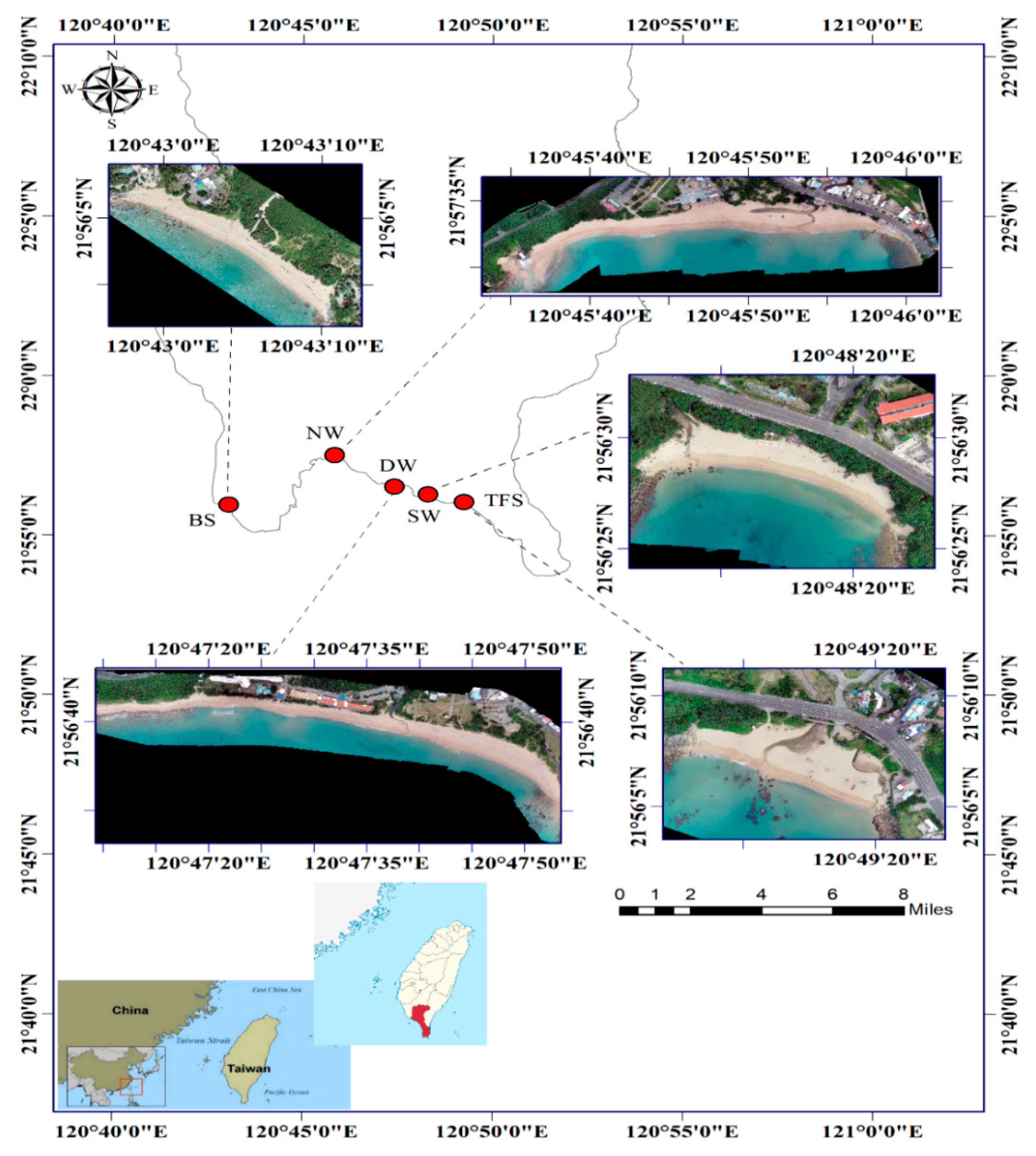
The study applied shoreline data collected from 5 beaches; Baisha (BS), Nanwan (NW), Big bay (DW), Little bay (SW), and Chuanfanshi (TFS), all of which were located in southern Taiwan, as shown in Figure 1 following the flowchart in Figure 2 for this study. The beaches are characterized by both fine and coarse sand. The spatial information on each beach is developed by using aerial survey maps provided by the Aerial Office of the Forestry Bureau for years 1982, 2002, 2006 [25], while serving as predictors while the unmanned aerial vehicle (UAV) surveyed data of 2019 serving as the respondent. The UAV model used was the Phantom 4 RTK (developed by Da-Jiang Innovations, DJI in Shenzhen, China) and a detailed description of the drone and the camera equipped may be found on the DJI website (https://www.dji.com/tw).
2.2. Artificial Neural Networks (ANNs)
ANNs have gained popularity in the last decades with successful applications in many fields such as sediment transport [16], satellite image classification [26], evapotranspiration [27], coastal erosion [28] etc. They are a very powerful computational technique for complex non-linear relationships. Their structure includes at least 3 layers; input, hidden, and output layers. Several ANNs have been developed; for example, the coactive neuro-fuzzy inference system model, recurrent network models, radial basis, multilayer perceptron, forward backpropagation, etc. In this study, however, we applied the multiple layer perceptron (MLP) due to the learning rule it applies, the backpropagation, which is an effective and practical learning algorithm [5,29].
Multilayer Perceptron Neural Network (MLP)
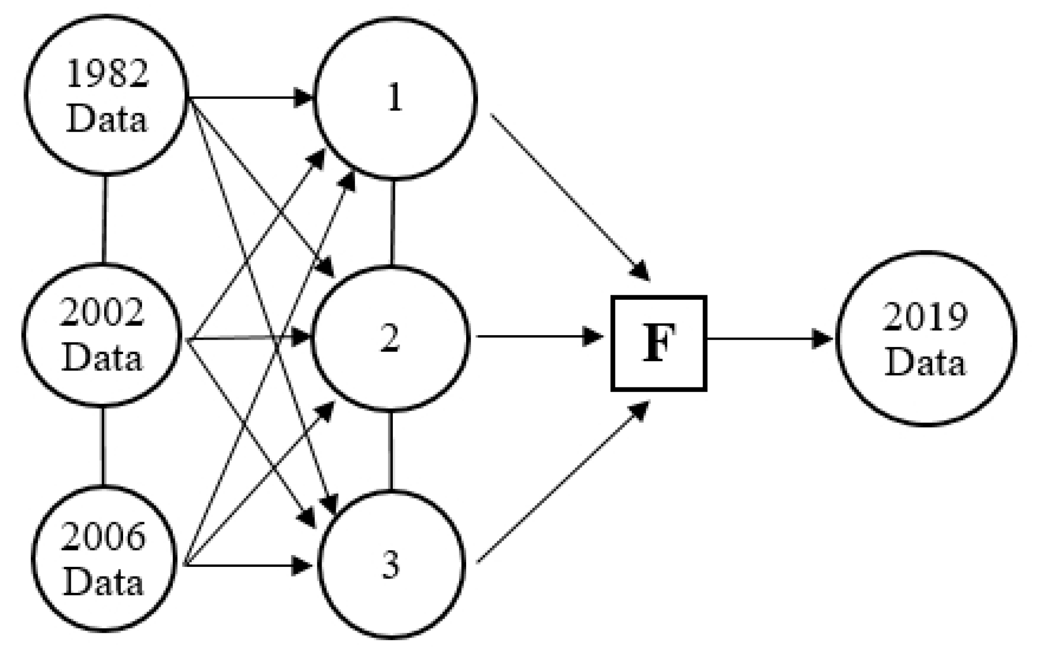
Multilayer perceptron (MLP) is characterized by the presence of one or more hidden layers, with computation connections called hidden neurons, whose function is to intervene between the external inputs and the network output in a useful manner. To extract high order statistics, more hidden layers may be added. The network acquires a global perspective despite its local connectivity due to the extrasynaptic connections and the extra dimension of neural network interconnections [30]. MLP may constitute more than a single hidden layer; moreover, previous studies have demonstrated a single layer to be adequate for most applications [31]. It is for this reason that this study employed one hidden layer. The equation for each MLP layer is shown in Equation (1). The structure of the model was basically a 3-3-1 as shown in Figure 3. Inputs of the model were 100 shoreline data points for 1982, 2002, and 2006, while 2019 was the predicted shoreline. Cömert and Kocamaz mentioned that before network training, it is necessary to understand the amount of data because of the size of the data neurons in the neural network. During the network evaluation, 70% of the data set is used for training, and the weights and deviations can be updated according to the network and the target output value; 15% is used for verification, so that the network stops training before overfitting occurs; 15% is used as testing to predict the performance of the network [32]. Therefore, these data were partitioned into 70% for training, 15% for validation and testing respectively [33,34]. Although there are several training algorithms, we applied the second-order Broyden–Fletcher–Goldfarb–Shanno algorithm with a maximum of 200 training cycles because of its high performance [35]. Learning rates and momentum were both fixed at 0.1 to avoid instabilities [36] and the weight decay fixed at 0.001. The model and all computations were performed through the platform of STATISTICA ver. 12.5 (by TIBCO, Hillview Avenue Palo Alto in USA).
where is the output of neuron j, is the connection weight from neuron i to neuron j, is the signal generated for neuron i, represents the bias associated with the neuron j and F(x) are the different activation functions which are discussed in the section below.
2.3. Activation Functions
Activation functions transform input signals from neurons of previous layers through mathematical functions, which may have a significant effect on the overall performance of a neural network model. Their overall function is to map any real input into a confined range, commonly from 0 to +1 or from −1 to +1. There are many types of activation functions, but the most commonly used include linear (sometimes referred to as identity) [37], logistic, hyperbolic tangent, Gaussian [38], threshold, sine functions, exponential linear unit, rectified linear units [39] etc. This study selected 5 activation functions (Identity, Tahn, Logistic, exponential and sine) to explore their impacts on a multilayer perceptron model. Their brief description is provided below.
2.3.1. Identity Function
This function returns a similar value used as its argument, simply obtained by the formula below:
where is observed coordinate Y-axis.
2.3.2. Hyperbolic Tan Function (Tanh)
Tahn is a symmetric s-shaped (sigmoid) function, whose output lies in the range (from −1 to +1) commonly used in MLP networks.
2.3.3. Logistic Function (Logistic)
This function differs from the Tahn function in that its output lies in the range (from 0 to +1). It is illustrated by the equation:
2.3.4. Exponential Function
The outputs of the function are from 0 to infinity. It is mostly applied when the target is positive.
2.3.5. Sine function
The sine function has a similar output range with the Tahn function, but is often used when the data being modeled is radially distributed.
2.4. Models Evaluation
In this study, the models were evaluated according to Liu et al. and Gupta et al. using two indices, the root mean square error (RMSE), and the Kling–Gupta efficiency (KGE), and the formulas are listed in Equations (7)–(9), respectively [7,40]. The RMSE is a measure of the residual variance while r is a measure of accuracy and is usually used to compare different models.
where represents the observed coordinate X axis, is the alternative methods-estimated coordinate X axis value; are the mean values of the equivalent parameter; and is the number of data under consideration. Additionally, a linear regression is applied for evaluating the models’ performance statistically, where y is the dependent variable (alternative methods), x the independent variable (observed), the slope, and the intercept. is the Euclidian distance from the ideal point, is the ratio between the standard deviation of simulated and the standard deviation of the observed coordinates, is the ratio between the mean simulated and mean observed coordinates, and represents the bias, can be interpreted as the potential value of KGE. The ideal value for KGE just like r is at unity.
3. Results and Discussion
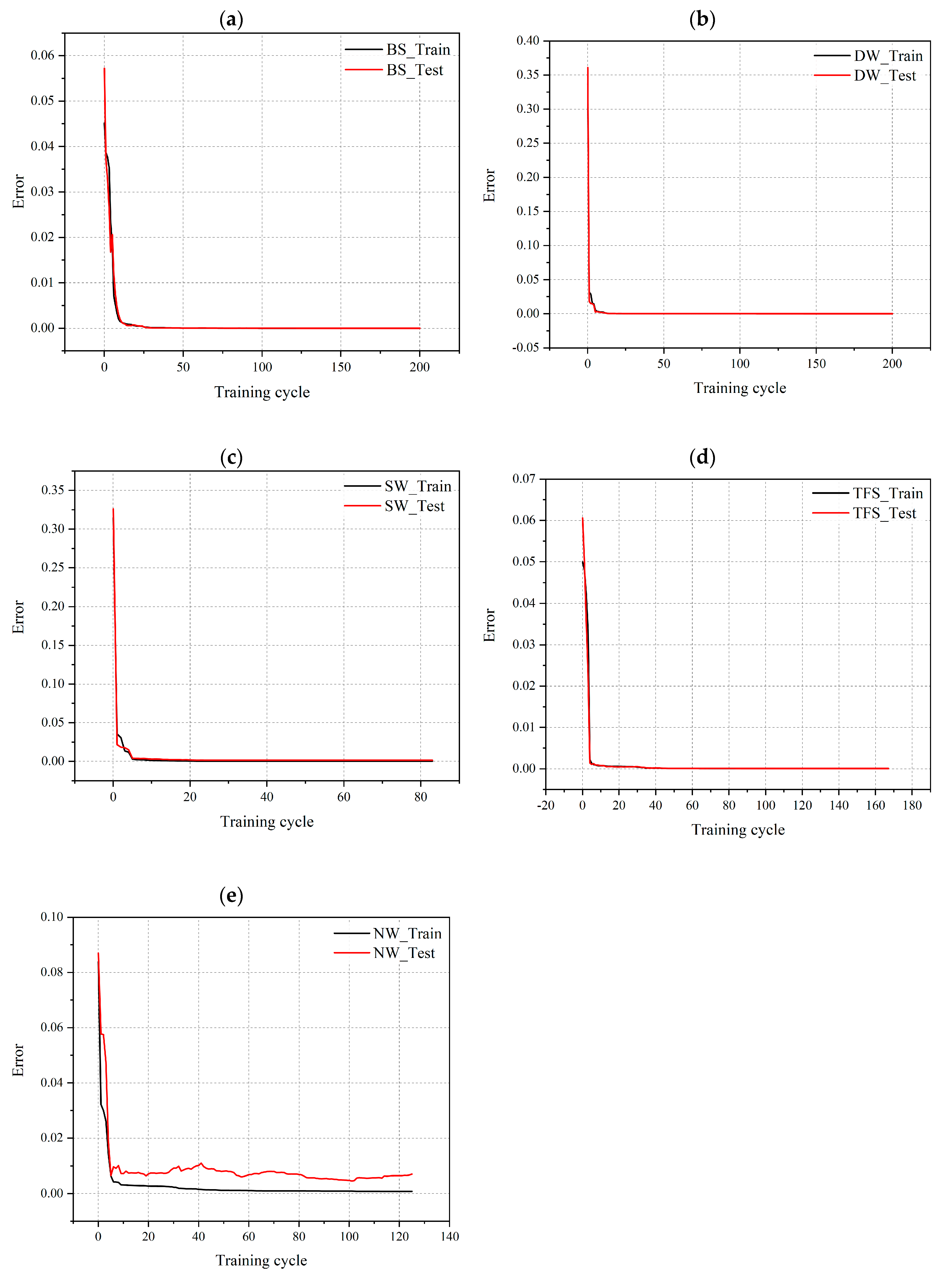
Table 1 shows the performance of the different activation functions in the five beaches. Logistic and Tahn activation functions are shown to have better overall performance, with higher r and KGE values and lower RMSE values. Logistic activation performed better at Baisha, Nanwan and Chuanfanshi, with r of respectively, 0.999, 0.983 and 0.999 during the testing phase. Similar patterns were observed with the KGE values, except for slight differences at Baisha and Nanwan. Due to the lower associated errors, reflected by the lower RMSE and bias value (), and the very slight differences between the r and KGE values, the Logistic activation function was still found to be better. Tahn performed best in the remaining beaches; Big Bay (r = 0.997) and Little Bay (r = 0.994). Training cycles and the respective errors during training and testing phases are shown in Figure 4. In all simulated cases, the errors follow a specific pattern, showing a significant drop with 5 training cycles. Some instabilities are observed however at NW using the logistic activation function. Deviating from observations made by Parascandolo et al. [41] who suggested that the Tahn function may be replaced by the Sine function, our results suggest that different functions may be applicable to specific scenarios or fields.
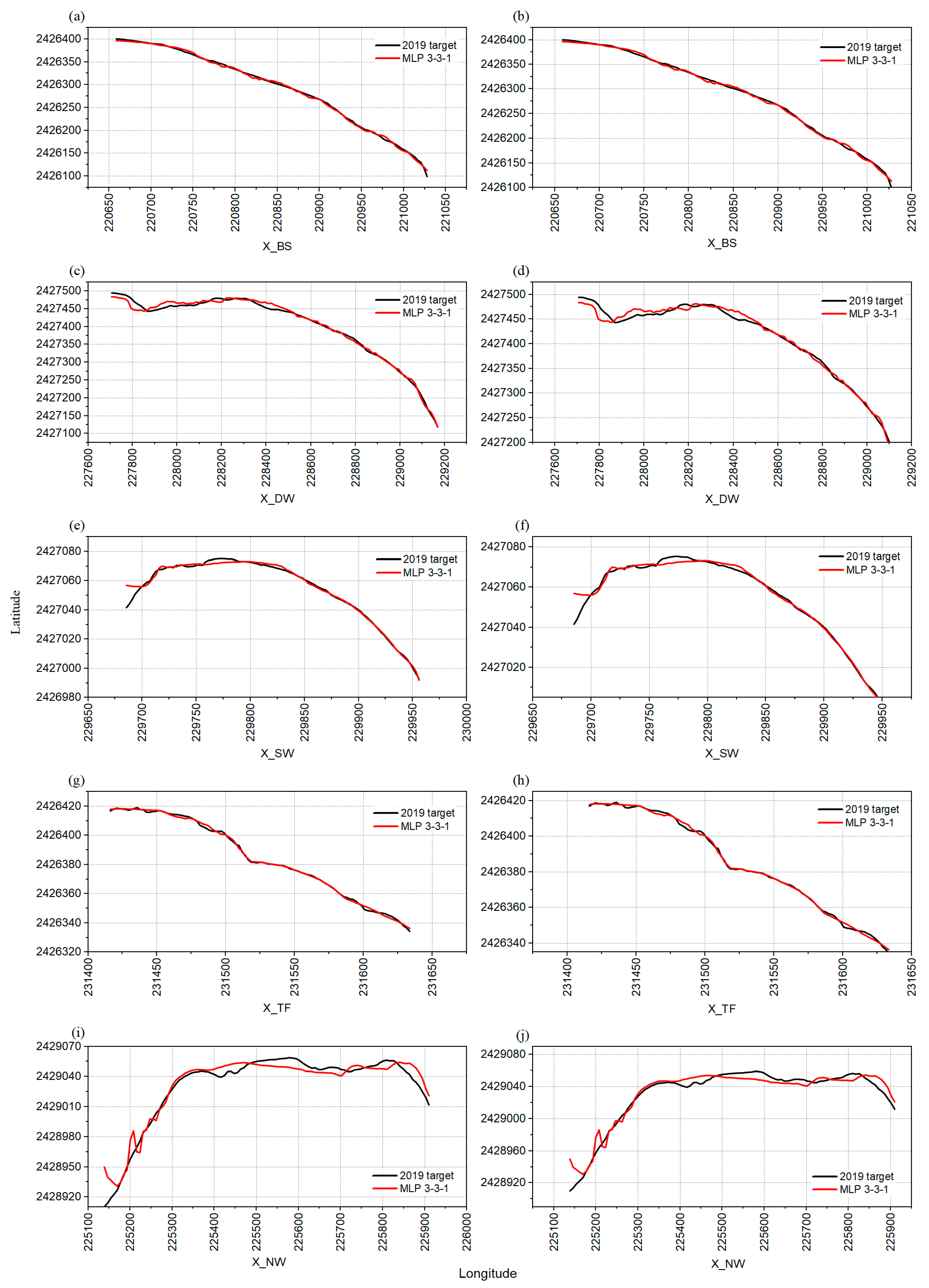
A visual of the estimated shoreline and the accuracy of the neural network in 2019 is further demonstrated in Figure 5. Prediction of the shoreline at NW is shown to be poorer than the other beaches. This is reflected by the higher errors during the testing cycle as shown in Figure 4. And the predicted change under both the training and the testing phases as can be found in Figure 5.
4. Conclusions
The knowledge of shoreline changes can play a crucial role in managing coastal areas, especially in storm-prone areas like Taiwan. The accurate prediction of such changes is also essential. The artificial neural network model applied (MLP) herein has demonstrated the application of artificial intelligence in this field. Additionally, the results have demonstrated the crucial role of activation functions in the application of such models. For modeling the shoreline change, different activation functions were considered. Logistic and Tahn functions were shown to perform better than Identity, Exponential and Sine Functions. The criteria used to select the best function were the highest R2 and the lowest RMSE. The findings serve as a valuable reference to the prediction of shorelines.
Author Contributions
Conceptualization, methodology and supervision, Y.-M.W.; analysis and writing J.-C.C. All authors have read and agreed to the published version of the manuscript.
Funding
This research was funded by Kenting National Park Headquarters (802-108-01-493).
Acknowledgments
The authors appreciate the anonymous reviewers for their constructive comments.
Conflicts of Interest
The authors declare no conflicts of interest.
References
- Papakonstantinou, A.; Topouzelis, K.; Pavlogeorgatos, G. Coastline Zones Identification and 3D Coastal Mapping Using UAV Spatial Data. ISPRS Int. J. Geo-Inf. 2016, 5, 75. [Google Scholar] [CrossRef] [Green Version]
- Neill, S.P.; Elliott, A.J.; Hashemi, M.R. A model of inter-annual variabilityin beach levels. Cont. Shelf Res. 2008, 28, 1769–1781. [Google Scholar] [CrossRef]
- Iglesias, G.; López, I.; Castro, A.; Carballo, R. Neural network modelling of planform geometry of headland-bay beaches. Geomorphology 2009, 103, 577–587. [Google Scholar] [CrossRef]
- Muñoz-Perez, J.J.; Medina, R. Comparison of long-, medium- and short-term variations of beach profiles with and without submerged geological control. Coast. Eng. 2010, 57, 241–251. [Google Scholar]
- López, I.; Aragonés, L.; Villacampa, Y.; Compañ, P. Artificial neural network modeling of cross-shore profile on sand beaches: The coast of the province of Valencia (Spain). Mar. Georesour. Geotechnol. 2017, 36, 698–708. [Google Scholar]
- Rodriguez-Delgado, C.; Bergillos, R.J.; Iglesias, G. An artificial neural network model of coastal erosion mitigation through wave farms. Environ. Model. Softw. 2019, 119, 390–399. [Google Scholar] [CrossRef]
- Liu, L.-W.; Wang, Y.-M. Modelling Reservoir Turbidity Using Landsat 8 Satellite Imagery by Gene Expression Programming. Water 2019, 11, 1479. [Google Scholar] [CrossRef] [Green Version]
- Yang, F.; Wanik, D.W.; Cerrai, D.; Bhuiyan, M.A.E.; Anagnostou, E.N. Quantifying Uncertainty in Machine Learning-Based Power Outage Prediction Model Training: A Tool for Sustainable Storm Restoration. Sustainability 2020, 12, 1525. [Google Scholar] [CrossRef] [Green Version]
- Cerrai, D.; Wanik, D.W.; Bhuiyan, M.A.E.; Zhang, X.; Yang, J.; Frediani, M.E.B.; Anagnostou, E.N. Predicting Storm Outages Through New Representations of Weather and Vegetation. IEEE Access 2019, 7, 29639–29654. [Google Scholar] [CrossRef]
- Bhuiyan, M.A.E.; Begum, F.; Ilham, S.J.; Khan, R.S. Advanced wind speed prediction using convective weather variables through machine learning application. Appl. Comput. Geosci. 2019, 1, 10002. [Google Scholar]
- Kumar, A.; Ramsankaran, R.A.A.J.; Brocca, L.; Munoz-Arriola, F. A Machine Learning Approach for Improving Near-Real-Time Satellite-Based Rainfall Estimates by Integrating Soil Moisture. Remote Sens. 2019, 11, 2221. [Google Scholar] [CrossRef] [Green Version]
- Hazra, A.; Maggioni, V.; Houser, P.; Antil, H.; Noonan, M. A Monte Carlo-based multi-objective optimization approach to merge different precipitation estimates for land surface modeling. J. Hydrol. 2019, 570, 454–462. [Google Scholar] [CrossRef]
- Bhuiyan, M.A.E.; Nikolopoulos, E.I.; Anagnostou, E.N.; Quintana-Seguí, P.; Barella-Ortiz, A. A nonparametric statistical technique for combining global precipitation datasets: Development and hydrological evaluation over the Iberian Peninsula. Hydrol. Earth Syst. Sci. 2018, 22, 1371–1389. [Google Scholar] [CrossRef] [Green Version]
- Zorzetto, E.; Marani, M. Extreme value metastatistical analysis of remotely sensed rainfall in ungauged areas: Spatial downscaling and error modelling. Adv. Water Resour. 2020, 135, 103483. [Google Scholar] [CrossRef]
- Jeatrakul, P.; Wong, K.W. Comparing the performance of different neural networks for binary classification problems. In Proceedings of the 2009 Eighth International Symposium on Natural Language Processing, Bangkok, Thailand, 20–22 October 2009; pp. 111–115. [Google Scholar]
- Tfwala, S.S.; Wang, Y.M. Estimating Sediment Discharge Using Sediment Rating Curves and Artificial Neural Networks in the Shiwen River, Taiwan. Water 2016, 8, 53. [Google Scholar] [CrossRef] [Green Version]
- Chen, S.M.; Wang, Y.M.; Tsou, I. Using artificial neural network approach for modelling rainfall-runoff due to typhoon. J. Earth Syst. Sci. 2013, 122, 399–405. [Google Scholar] [CrossRef] [Green Version]
- Wang, Y.M.; Traore, S.; Kerh, T.; Leu, J.M. Modelling Reference Evapotranspiration Using Feed Forward Backpropagation Algorithm in Arid Regions of Africa. Irrig. Drain. 2011, 60, 404–417. [Google Scholar] [CrossRef]
- Awolusi, T.F.; Oke, O.L.; Akinkurolere, O.O.; Sojobi, A.O.; Aluko, O.G. Performance comparison of neural network training algorithms in the modeling properties of steel fiber reinforced concrete. Heliyon 2019, 5, e01115. [Google Scholar] [CrossRef] [Green Version]
- Wang, Y.M.; Traore, S. Time-lagged recurrent network for forecasting episodic event suspended sediment load in typhoon prone area. Int. J. Phys. Sci. 2009, 4, 519–528. [Google Scholar]
- Sentas, A.; Psilovikos, A. Comparison of ARIMA and transfer function (TF) models in water temperature simulation in dam-lake Thesaurus, eastern Macedonia, Greece. In Proceedings of the International Symposium: Environmental Hydraulics, Athens, Greece, 23–25 June 2010; pp. 929–934. [Google Scholar]
- Afzaal, H.; Farooque, A.A.; Abbas, F.; Acharya, B.; Esau, T. Groundwater Estimation from Major Physical Hydrology Components Using Artificial Neural Networks and Deep Learning. Water 2019, 12, 5. [Google Scholar] [CrossRef] [Green Version]
- Zubier, K.M.; Eyouni, L.S. Investigating the role of atmospheric variables on sea level variations in the eastern central red sea using an artificial neural network approach. Oceanologia 2020. [Google Scholar] [CrossRef]
- Karamoutsou, L.; Psilovikos, A. The use of artificial neural network in water quality prediction in lake Kastoria, Greece. In Proceedings of the 14th Conference of the Hellenic Hydrotechnical Association (H.H.A.), Volos, Greece, 16–17 May 2019. [Google Scholar]
- Kerh, T.; Hsu, G.S.; Gunaratnam, D. Forecasting of Nonlinera Shoreline Variation Based on Aerial Survey Map by Nueral Network Approach. Int. J. Nonlinear Sci. Numer. Simul. 2009, 10, 1211–1222. [Google Scholar] [CrossRef]
- Manaf, S.A.; Mustapha, N.; Sulaiman, M.N.; Husin, N.A.; Hamid, M.R.A. Artificial Neural Networks for Satellite Image Classification of Shoreline Extraction for Land and Water Classes of the North West Coast of Peninsular Malaysia. Adv. Sci. Lett. 2018, 24, 1382–1387. [Google Scholar] [CrossRef]
- Kariyama, I.D. Temperature Based Feed Forward Backpropagation Artificial Neural Network for Estimating Reference Crop Evapotranspiration in the Upper West Region. Int. J. Sci. Technol. Res. 2014, 3, 357–364. [Google Scholar]
- Peponi, A.; Morgado, P.; Trindade, J. Combining Artificial Neural Networks and GIS Fundamentals for Coastal Erosion Prediction Modeling. Sustainability 2019, 11, 975. [Google Scholar] [CrossRef] [Green Version]
- Khotanzad, A.; Chung, C. Application of multi-layer perceptron neural networks to vision problems. Neural Comput. Appl. 1998, 7, 249–259. [Google Scholar] [CrossRef]
- Tfwala, S.S.; Wang, Y.-M.; Lin, Y.-C. Prediction of Missing Flow Records Using Multilayer Perceptron and Coactive Neurofuzzy Inference System. Sci. World J. 2013, 2013, 1–7. [Google Scholar] [CrossRef] [Green Version]
- Chi, Y.N.; Chi, J. Saltwater anglers toward marine environmental threats using multilayer perceptron neural network framework. Int. J. Data Sci. Adv. 2020, 2, 6–17. [Google Scholar]
- Cömert, Z.; Kocamaz, A.F. A study of artificial neural network training alorithms classification of cardiotocography signals. Bitlis Eren Univ. J. Sci. Technol. 2017, 7, 93–103. [Google Scholar]
- Kulp, S.A.; Strauss, B.H. Coastaldem: A global coastal digital elevation model improved from SRTM using a neural network. Remote Sens. Environ. 2018, 206, 231–239. [Google Scholar] [CrossRef]
- Fernández, J.R.M.; Vidal, J.d.l.C.B. Fast selection of the sea clutter preferential distribution with neural networks. Eng. Appl. Artif. Intell. 2018, 70, 123–129. [Google Scholar] [CrossRef]
- Saputro, D.R.S.; Widyaningsih, P. Limited memory Broyden-Fletcher-Goldfarb-Shanno (L-BFGS) method for the parameter estimation on geographically weighted ordinal logistic regression model (GWOLR). AIP Conf. Proc. 2017, 1868, 040009. [Google Scholar]
- Attoh-Okine, N.O. Analysis of learning rate and momentum term in backpropagation neural network algorithm trained to predict pavement performance. Adv. Eng. Softw. 1999, 30, 291–302. [Google Scholar] [CrossRef]
- Arminger, G.; Enache, D. Statistical models and artificial neural networks. In Data Anaysis and Information Systems; Bock, H.-H., Polasek, W., Eds.; Springer: Berlin/Heidelberg, Germany, 1996; pp. 243–260. [Google Scholar]
- Urban, S.; Basalla, M.; van der Smagt, P. Available online: https://arxiv.org/abs/1711.11059.pdf (accessed on 25 March 2020).
- Glorot, X.; Bordes, A.; Bengio, Y. Available online: http://proceedings.mlr.press/v15/glorot11a/glorot11a.pdf (accessed on 25 March 2020).
- Gupta, H.V.; Kling, H.; Yilmaz, K.K.; Martinez, G.F. Decomposition of the mean squared error and NSE performance criteria: Implications for improving hydrological modelling. J. Hydrol. 2009, 377, 80–91. [Google Scholar] [CrossRef] [Green Version]
- Parascandolo, G.; Huttunen, H.; Virtanen, T. Available online: https://openreview.net/forum?id=Sks3zF9eg (accessed on 25 March 2020).
Figure 1.
Location and images of the five beaches collected by the unmanned aerial vehicle (UAV).

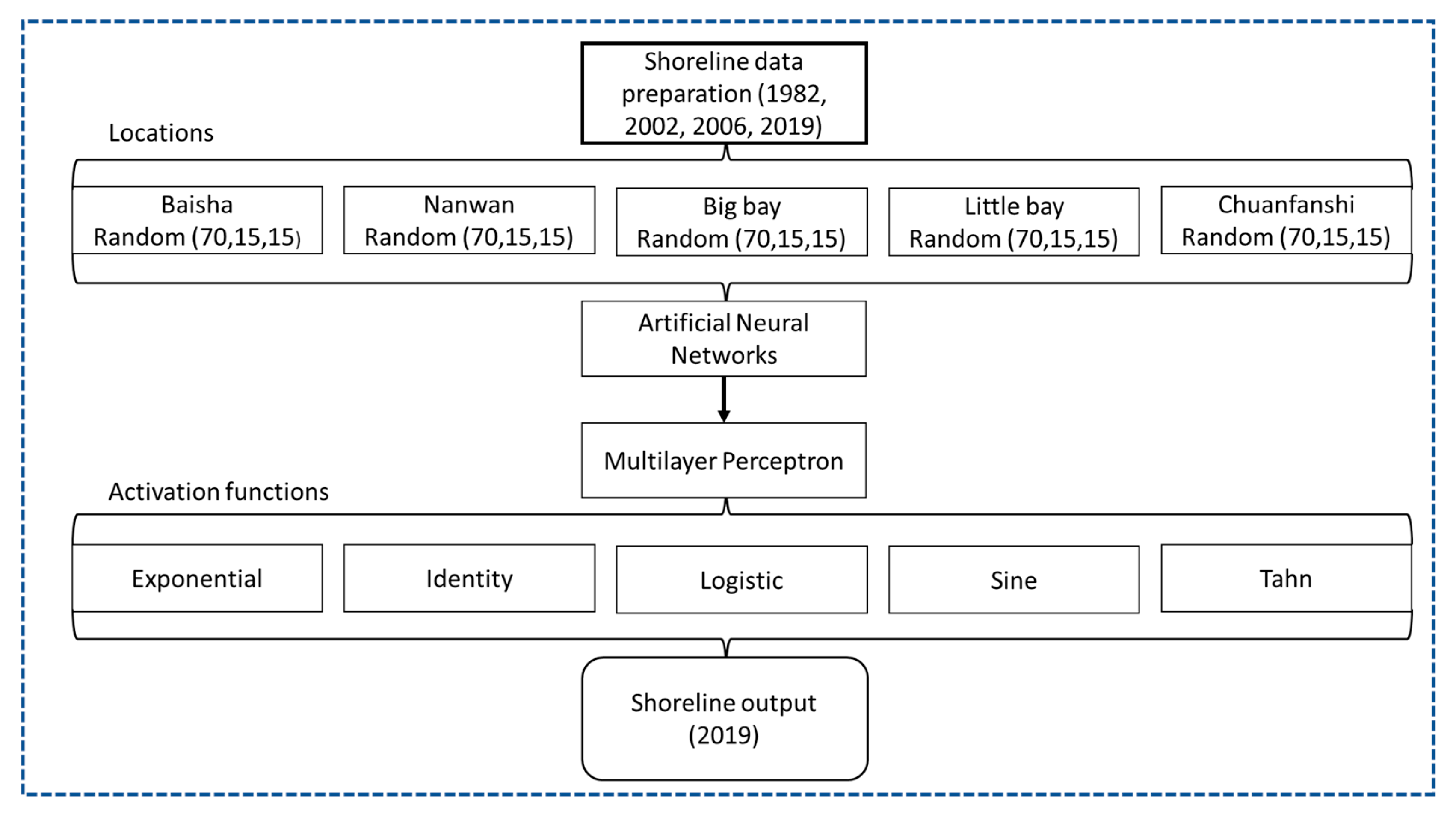
Figure 2.
Flow chart of the study.

Figure 3.
Architecture of the multilayer perceptron network.

Figure 4.
(a–e) Training cycles and errors of the different activation functions.

Figure 5.
Observed and predicted shoreline changes in training (a,c,e,g,i) and testing (b,d,f,h,j) phases of the best performing activation functions (Logistic and Tahn).
Figure 5.
Observed and predicted shoreline changes in training (a,c,e,g,i) and testing (b,d,f,h,j) phases of the best performing activation functions (Logistic and Tahn).


Table 1.
Performance of the different activation functions.
| Location | Function | Training | Validation | Testing | ||||||||||||
|---|---|---|---|---|---|---|---|---|---|---|---|---|---|---|---|---|
| RMSE | KGE | r | RMSE | KGE | r | RMSE | KGE | r | ||||||||
| BS | Exponential | 4.092 | 0.995 | 0.999 | 1.000 | 1.005 | 1.963 | 0.991 | 0.999 | 1.000 | 0.991 | 4.092 | 0.973 | 1.000 | 1.000 | 0.973 |
| Identity | 4.944 | 0.961 | 0.994 | 1.000 | 1.039 | 5.099 | 0.962 | 0.997 | 1.000 | 1.038 | 3.912 | 0.987 | 0.995 | 1.000 | 1.012 | |
| Logistic | 3.195 | 0.995 | 0.999 | 1.000 | 1.005 | 2.856 | 0.993 | 0.999 | 1.000 | 0.993 | 3.153 | 0.988 | 0.999 | 1.000 | 0.988 | |
| Sine | 8.685 | 0.961 | 0.994 | 1.000 | 1.039 | 7.712 | 0.962 | 0.997 | 1.000 | 1.038 | 6.653 | 0.987 | 0.995 | 1.000 | 1.012 | |
| Tahn | 7.003 | 0.977 | 0.996 | 1.000 | 1.023 | 7.411 | 0.996 | 0.997 | 1.000 | 0.997 | 6.587 | 0.995 | 0.996 | 1.000 | 0.998 | |
| DW | Exponential | 11.318 | 0.973 | 0.992 | 1.000 | 1.026 | 5.093 | 0.978 | 0.995 | 1.000 | 1.022 | 9.479 | 0.995 | 0.998 | 1.000 | 0.996 |
| Identity | 13.914 | 0.985 | 0.994 | 1.000 | 1.014 | 5.572 | 0.978 | 0.996 | 1.000 | 1.021 | 12.153 | 0.983 | 0.993 | 1.000 | 1.016 | |
| Logistic | 9.042 | 0.989 | 0.995 | 1.000 | 1.010 | 8.531 | 0.987 | 0.997 | 1.000 | 1.013 | 8.120 | 0.993 | 0.994 | 1.000 | 0.996 | |
| Sine | 9.820 | 0.985 | 0.994 | 1.000 | 1.014 | 8.812 | 0.978 | 0.996 | 1.000 | 1.021 | 8.330 | 0.983 | 0.993 | 1.000 | 1.016 | |
| Tahn | 8.459 | 0.996 | 0.996 | 1.000 | 1.002 | 8.210 | 0.985 | 0.997 | 1.000 | 0.985 | 7.782 | 0.994 | 0.994 | 1.000 | 1.001 | |
| NW | Exponential | 7.504 | 0.951 | 0.975 | 1.000 | 1.042 | 6.303 | 0.763 | 0.981 | 1.000 | 1.237 | 6.647 | 0.794 | 0.988 | 1.000 | 1.205 |
| Identity | 14.263 | 0.932 | 0.969 | 1.000 | 1.061 | 10.096 | 0.798 | 0.972 | 1.000 | 1.200 | 17.322 | 0.702 | 0.985 | 1.000 | 1.298 | |
| Logistic | 6.513 | 0.968 | 0.982 | 1.000 | 1.027 | 6.955 | 0.741 | 0.985 | 1.000 | 1.258 | 5.898 | 0.716 | 0.983 | 1.000 | 1.284 | |
| Sine | 8.100 | 0.932 | 0.969 | 1.000 | 1.061 | 6.400 | 0.798 | 0.972 | 1.000 | 1.200 | 8.295 | 0.702 | 0.985 | 1.000 | 1.298 | |
| Tahn | 7.031 | 0.970 | 0.981 | 1.000 | 1.023 | 7.01913 | 0.854 | 0.969 | 1.000 | 1.143 | 8.179 | 0.870 | 0.983 | 1.000 | 1.129 | |
| SW | Exponential | 1.489 | 0.996 | 0.998 | 1.000 | 1.004 | 5.283 | 0.972 | 0.986 | 1.000 | 1.024 | 3.995 | 0.942 | 0.957 | 1.000 | 1.039 |
| Identity | 1.751 | 0.968 | 0.994 | 1.000 | 1.032 | 5.570 | 0.946 | 0.979 | 1.000 | 1.050 | 4.280 | 0.913 | 0.942 | 1.000 | 1.065 | |
| Logistic | 1.693 | 0.991 | 0.997 | 1.000 | 1.008 | 5.113 | 0.966 | 0.987 | 1.000 | 1.032 | 3.751 | 0.950 | 0.960 | 1.000 | 1.031 | |
| Sine | 2.351 | 0.968 | 0.994 | 1.000 | 1.032 | 5.927 | 0.946 | 0.979 | 1.000 | 1.050 | 4.670 | 0.913 | 0.942 | 1.000 | 1.065 | |
| Tahn | 1.417 | 0.997 | 0.998 | 1.000 | 1.003 | 4.052 | 0.984 | 0.991 | 1.000 | 1.014 | 3.181 | 0.960 | 0.973 | 1.000 | 1.029 | |
| TFS | Exponential | 1.155 | 0.998 | 0.999 | 1.000 | 1.002 | 1.326 | 0.998 | 0.999 | 1.000 | 0.999 | 1.206 | 0.987 | 0.999 | 1.000 | 0.994 |
| Identity | 2.190 | 0.969 | 0.985 | 1.000 | 0.973 | 2.194 | 0.979 | 0.985 | 1.000 | 1.015 | 2.505 | 0.942 | 0.985 | 1.000 | 1.056 | |
| Logistic | 1.051 | 0.999 | 0.999 | 1.000 | 0.999 | 0.982 | 0.999 | 1.000 | 1.000 | 1.001 | 0.916 | 0.994 | 0.999 | 1.000 | 0.987 | |
| Sine | 4.735 | 0.969 | 0.985 | 1.000 | 0.973 | 4.297 | 0.979 | 0.985 | 1.000 | 1.015 | 5.104 | 0.942 | 0.985 | 1.000 | 1.056 | |
| Tahn | 1.550 | 0.998 | 0.998 | 1.000 | 0.998 | 1.599 | 0.986 | 0.999 | 1.000 | 1.014 | 1.537 | 0.983 | 0.998 | 1.000 | 1.017 | |
© 2020 by the authors. Licensee MDPI, Basel, Switzerland. This article is an open access article distributed under the terms and conditions of the Creative Commons Attribution (CC BY) license (http://creativecommons.org/licenses/by/4.0/).
Share and Cite
MDPI and ACS Style
Chen, J.-C.; Wang, Y.-M. Comparing Activation Functions in Modeling Shoreline Variation Using Multilayer Perceptron Neural Network. Water 2020, 12, 1281. https://doi.org/10.3390/w12051281
AMA Style
Chen J-C, Wang Y-M. Comparing Activation Functions in Modeling Shoreline Variation Using Multilayer Perceptron Neural Network. Water. 2020; 12(5):1281. https://doi.org/10.3390/w12051281
Chicago/Turabian StyleChen, Je-Chian, and Yu-Min Wang. 2020. "Comparing Activation Functions in Modeling Shoreline Variation Using Multilayer Perceptron Neural Network" Water 12, no. 5: 1281. https://doi.org/10.3390/w12051281
Note that from the first issue of 2016, this journal uses article numbers instead of page numbers. See further details here.