Consistent Boundary Conditions for Age Calculations
by
 , , ,
, , ,
Eric Deleersnijder
1 ,
,
Insaf Draoui
2,* ,
,
Jonathan Lambrechts
2,
Vincent Legat
2 and
Anne Mouchet
3 1
Institute of Mechanics, Materials and Civil Engineering (IMMC) & Earth and Life Institute (ELI) L4.05.02, Université Catholique de Louvain, B-1348 Louvain-la-Neuve, Belgium
2
Institute of Mechanics, Materials and Civil Engineering (IMMC), Université Catholique de Louvain, L4.05.02, B-1348 Louvain-la-Neuve, Belgium
3
Freshwater and OCeanic science Unit of reSearch (FOCUS), Sart-Tilman B5a, Université de Liège, B-4000 Liège, Belgium
*
Author to whom correspondence should be addressed.
Water 2020, 12(5), 1274; https://doi.org/10.3390/w12051274
Submission received: 18 March 2020
/
Revised: 22 April 2020
/
Accepted: 27 April 2020
/
Published: 30 April 2020
(This article belongs to the Special Issue Tracer and Timescale Methods for Passive and Reactive Transport in Fluid Flows)
Abstract
:Age can be evaluated at any time and position to understand transport processes taking place in the aquatic environment, including for reactive tracers. In the framework of the Constituent-oriented Age and Residence time Theory (CART), the age of a constituent or an aggregate of constituents, including the water itself, is usually defined as the time elapsed since leaving the boundary where the age is set or reset to zero. The age is evaluated as the ratio of the age concentration to the concentration, which are the solution of partial differential equations. The boundary conditions for the concentration and age concentration cannot be prescribed independently of each other. Instead, they must be derived from boundary conditions designed beforehand for the age distribution function (the histogram of the ages, the age theory core variable), even when this variable is not calculated explicitly. Consistent boundary conditions are established for insulating, departure and arrival boundaries. Gas exchanges through the water–air interface are also considered. Age fields ensuing from consistent boundary conditions and, occasionally, non-consistent ones are discussed, suggesting that the methodology advocated herein can be utilized by most age calculations, be they used for diagnosing the results of idealised models or realistic ones.
1. Introduction
Today’s numerical models of geophysical and environmental fluid flows and the related (reactive) transport processes produce huge output files. Making sense of all these real numbers (that is, identifying key processes and establishing causal relationships between them) is no trivial task. Analysing primitive variables (e.g., velocity, pressure, temperature, concentrations) is not always conducive to the most fruitful interpretations. Evaluating auxiliary variables introduced for diagnostic purposes is an option worth considering. In this respect, diagnostic timescales (e.g., age, transit time, residence or exposure time) have been of use in the modelling of the atmosphere [1,2,3,4], various types of water bodies [5,6,7,8,9,10,11,12,13,14,15,16,17,18,19,20,21,22,23,24,25,26,27,28,29,30,31,32,33,34,35,36,37,38,39,40,41,42,43,44,45,46,47,48,49], and sediment transport [39,50,51,52]. These diagnostic timescales paint a simplified picture of the impact that the phenomena under study have on the largest time and space scales of (reactive) transport.
The residence or exposure time [16,53] and the age are of fundamentally different natures, as may be seen, for instance, in figure 13 of [54]. The former type of timescale looks into the future, whilst the age is concerned with the past evolution. The present study deals with age calculations.
Age and age-related variables were introduced for zero-dimensional (or reservoir) modelling by Bolin and Rodhe [55]. Then, Zimmerman [54] and Takeoka [56] paved the way for theories allowing the age to be calculated numerically at every time and location from numerical model results [57,58,59,60]. With this approach, most, if not all of the numerical results are taken into account, which is why the ensuing timescale fields may be considered holistic.
Deleersnijder [61] made an attempt at building the most general definition of the age. The latter is as follows: the age of a particle of a constituent of seawater is the time that has elapsed since it began to be taken into consideration. In many cases, particles begin to be taken into consideration at the instant they enter the domain of interest, in which case the age is the time elapsed since entering the domain (e.g., [54,56,62]). When reactions are present, it may be found to be appropriate to transfer the age from one constituent to another [63]. Other age calculation strategies exist, in which, for instance, the age is evaluated as the time elapsed since leaving the sea bottom or surface [57,58,64,65,66,67]. Where and how particles cease to be considered must also be specified. All of these considerations clearly point to the importance of the boundary conditions.
The fate of a single particle is rather irrelevant [68]—a sufficiently large number of particles must be taken into consideration. As a consequence, the mean age of a set of particles must be introduced. In accordance with the age-averaging hypothesis [69], the mean age is defined as follows [61]: the mean age of a collection of particles is the mass-weighted average of their individual ages.
The mean age, which, for simplicity, will be called "age" hereinafter, may be computed at every time and location in the Lagrangian framework or in the Eulerian one. The Constituent-oriented Age and Residence time Theory (CART, www.climate.be/cart) is an Eulerian approach to the calculation of the age of any constituent of the water, or groups of constituents (that is, aggregates), including the water itself [59,69,70]. The age is obtained as the ratio of the age concentration to the concentration of the constituent or aggregate under consideration. These variables are the solutions of coupled reactive transport equations. The initial and boundary conditions must be prescribed in accordance with the declared objectives of the diagnostic strategy. So far, insufficient attention has been paid to the formulation of the boundary conditions. Specifically, one has yet to make it clear that the boundary conditions for the concentration and age concentration cannot be built independently of each other and draw the relevant consequences. Filling this gap is the objective of the present study.
In Section 2, we recall the definition of the age concentration function and evaluate its first two moments, the concentration and age concentration, so as to obtain the mean age. No novel concept is introduced in this section, but developments of the past two decades are taken into account, hopefully yielding a line of reasoning that is easy to comprehend. This should facilitate the understanding of the strategy for building boundary conditions that is set out in Section 3, in which various types of boundaries are considered, that is, insulating, arrival, and departure boundaries, as well as semi-permeable boundaries allowing gas exchanges between water and air. In Section 4, the results of the preceding section are put into perspective by tackling a simple ventilation assessment problem. Conclusions are drawn in Section 5.
2. The Age Distribution Function and Its First Two Moments
Although it is possible to apply CART to compressible fluid flows, this conceptual toolbox has been used thus far exclusively in the framework of the Boussinesq approximation. Therefore, the density of the fluid (that is, a mixture of pure water and many other constituents), , is assumed to be constant. Let denote the position vector, where x, y, and z are Cartesian coordinates. In accordance with the continuous media approach, the relevant variables are introduced in relation to elemental control volumes. We denote and as the elemental control domain located at and the value of its volume, respectively.
As far as the age is concerned, CART’s core variable is the age distribution function [59,71], where independent variables t and denote the time and the age, respectively. The latter is generally assumed to be positive definite, that is, . Function is defined as follows: in the abovementioned control volume, at time t, the mass of the particles of the constituent under study whose age lies in the interval tends to as . Clearly, the physical dimension of the age distribution function is , and this function may be viewed as the histogram of the particle ages at time t and location . Advection and diffusion proceed independently of the age of the particles being transported. Then, by having recourse to mass conservation considerations alone, Delhez et al. [59] established the equation governing the age distribution function, which reads:
where ∇, , and denote the del operator, the fluid velocity, and the diffusivity tensor, respectively. Under the Boussinesq approximation, the velocity is divergence-free, that is, . As was argued in Appendix A of Deleersnijder et al. [69], the diffusivity tensor must be symmetric and positive-definite. Equation (1) holds valid for a passive or inert constituent (also termed tracer). By adding suitable production-destruction terms, it can be extended to take reactions into account [59]. Doing so is, however, not necessary to serve the purpose of the present study. The last term in Equation (1) is related to ageing. It may be seen as an advection term related to a unit velocity, representing the fact that the age tends to increase at the same pace as time progresses.
The mass of the constituent under study that is present in elemental control volume is obtained by taking the sum over all age categories, that is,
where is the mass of the fluid present in under the Boussinesq approximation. Then, the concentration of the constituent under consideration, defined as a mass fraction (that is, a dimensionless variable), reads:
which means that the concentration is the 0th order moment of the age distribution function. By integrating (1) over the age, Delhez et al. [59] obtained the well-known advection-diffusion equation governing the evolution of the concentration:
The age content of a particle [69] is defined as the product of its age and mass. Like mass, this quantity is of an additive nature. As a consequence, the age content of the particles of the constituent under study that are present in is:
This points to the importance of the first-order moment of the age distribution function,
which, in the CART-related literature, is termed age concentration. Delhez et al. [59] established the equation obeyed by by multiplying (1) by the age and integrating over the age, eventually yielding:
Owing to its relation to the age content, the age concentration is an extensive variable. This is why it is no surprise that it satisfies a reactive transport equation. The last term in the right-hand side of (7) is related to ageing. It is through this term that the equations for the concentration and age concentration are coupled.
Concentration and age concentration Equations (4) and (7) are of a parabolic nature [72]. Therefore, to solve each of them, the initial value of their solution must be prescribed and one boundary condition has to be enforced at every point of the surface delimiting the domain of interest.
According to the abovementioned age-averaging hypothesis [69], the mean age of the particles under study that are present in is:
This type of averaging is not the only one that can be conceived. The choice that has been made is the only arbitrary ingredient in the developments leading to CART’s age. As opposed to the concentration and age concentration, the age is an intensive variable, rather than an extensive one. In contrast with the equations for C and , the equation obeyed by the age, which is obtained by combining (1), (7) and (8),
cannot be cast into a conservative form. This is why in most, if not all numerical studies, the mean age has been computed as the ratio of the age concentration to the concentration rather than by solving the age Equation (9) [39,47,65,69,73,74,75,76,77,78,79,80,81,82,83,84,85,86,87,88]. This equation may, however, prove to be useful in theoretical studies [89,90,91].
In the right-hand side of relation (9), the first term is associated with ageing, whilst the second one bears some similarity with an advection term. However, the expression that may be regarded as the velocity, , is not divergence-free. Its behaviour is at the root of the intriguing symmetry that the age field occasionally exhibits [89,91,92,93].
A number of studies focused on seawater, which may be split into several water types, components, or masses (though the word “type” is likely to be more appropriate in this instance), which can be treated as inert tracers [15,60,62,69,94,95]. Obviously, the diagnostic strategy must be designed in such a way that the sum of all the water type concentrations must be equal to a constant at any time and location. With no loss of generality, this constant may be assumed to be equal to unity. For a tracer with unit concentration, age Equation (9) simplifies to the equation solved by England [58], and the corresponding age is sometimes called ventilation, or ideal age.
3. Consistent Insulating, Departure, and Arrival Boundary Conditions
Numerically solving the equation for the distribution function presents several challenges. First, there is an additional independent variable, namely, the age (). For example, if the three space dimensions are taken into account, Equation (1) must be discretised in a five-dimensional space, the corresponding independent variables of which are t, x, y, z, and . The necessary numerical developments are not trivial and the added computational cost cannot go unnoticed [71]. Furthermore, when the distribution function exhibits a long tail, Cornaton [96] argued that standard numerical techniques are no longer appropriate, which is why he developed a method involving the Laplace transform and classical space-time discretisations. This technique is computationally efficient, but its implementation is not straightforward.
Most authors did not find it necessary to compute the age distribution function and, instead, focused on the (mean) age, obtained from the solution of the concentration and age concentration equations. These equations are to be solved under boundary conditions that must be consistent with each other. They should be derived from the boundary conditions that the age distribution function would obey if the equation governing this function was to be solved explicitly. Accordingly, we will derive a number of consistent boundary conditions, illustrate their impact on relevant problems and, when appropriate, show that opting for inconsistent boundary conditions would have a detrimental impact on the age field. Schematically, we will address insulating, departure, and arrival boundaries. We will also consider gas exchanges through the water–air interface.
Though the illustrations below essentially deal with passive constituents, the developments leading to consistent boundary conditions apply to any type of constituent, which includes constituents undergoing reactions.
3.1. Insulating Boundary
Consider surface , whose outward unit normal is denoted . Assume that this surface is impermeable, thereby insulating the neighbouring part of the domain of interest from its environment. As a result, the velocity satisfies boundary condition
Since this boundary is impermeable, no particles of the constituent under consideration, irrespective of their age, cross it, leading to
Combining (10) and (11) yields
To derive the boundary condition for the concentration, we integrate (12) over the age and use relation (3):
Multiplying (12) by , integrating over and using definition (6) of the age concentration, we obtain
Unsurprisingly, and obey zero normal diffusive flux boundary conditions.
Boundary conditions (12)–(14) may be cast into generic form , where is the variable whose diffusive flux is zero through the boundary. If is parallel to one of the principal axes of the diffusivity tensor, then such a boundary condition simplifies to . For instance, assume that the diffusivity tensor takes the widely-used form of , where and are the horizontal diffusivity and the vertical one, respectively. If the boundary under consideration is horizontal, then the aforementioned zero normal flux boundary condition degenerates into , where z denotes the vertical coordinate.
Now, for illustration purposes, assume that the domain of interest, , is completely insulated from its environment, implying that the abovementioned boundary conditions are to be enforced on the whole boundary (Figure 1). Further assume that the age of all the particles of a passive tracer is zero at the initial time, that is, , where and are the initial concentration field and the Dirac delta function, respectively. The corresponding initial age concentration is readily seen to be . Then, at any point of and time , the age distribution function is , implying that the age concentration and the age are and . This result is readily understood. No particles enter or leave the domain. As all particles age at the same pace as time progresses, their age is equal to the elapsed time. The aforementioned results, and , can also be obtained without computing the age distribution function and, instead, by solving only the concentration and age concentration equations under boundary conditions (13) and (14). This is readily seen.
In this case study, that the age is equal to the elapsed time is of little diagnostic value. However, it may be regarded as a piece of information supporting the well-foundedness of boundary conditions (13) and (14). In other words, these boundary conditions allow us to obtain the expected result. Opting for another set of boundary conditions would lead to an unacceptable age field.
We should note in passing that, had we studied the evolution of a tracer undergoing a first-order decay process associated with constant mean life (and, hence, half-life ), we would have obtained the following result: , and , where subscript “d” identifies the fields related to the decaying tracer. As a consequence, the age would have been unchanged: . This is chiefly because first-order decay proceeds at the same rate at every time and position [19,97].
3.2. Departure Boundary
If the age is defined as the time elapsed since leaving a given boundary, then the age of all the particles under consideration must be set or reset to zero at the moment they touch this boundary, leading to
where, in this subsection, refers to the departure boundary (that is, the boundary where the age is prescribed to be zero), which is usually a fraction of the domain boundary; is the tracer concentration on departure boundary , which is assumed to be known (Dirichlet boundary condition). The boundary condition for the age concentration is derived from (15) as follows:
Thus, the concentration and age concentration obey Dirichlet boundary conditions.
To help understand the role of these boundary conditions, consider a one-dimensional flow, in semi-infinite domain (Figure 2). The age of a passive tracer particle is defined as the time elapsed since leaving the departure boundary (). At the initial instant (), there is no tracer in the domain and the tracer concentration is prescribed to be equal to constant on the departure boundary. If positive constants U and K represent the velocity and the diffusivity, the equation obeyed by age distribution function is
This equation is to be solved under the following initial and boundary conditions
Without any loss of generality, may be assumed to be equal to unity. Accordingly, the solution reads (Figure 3)
where is the Heaviside step function, that is, function is equal to unity (resp. zero) according to whether (resp. ).
The concentration of the tracer is
whilst its age concentration reads
The related age, , may be seen to be smaller than the elapsed time, as it should be.
It is noteworthy that the (mean) age could have been obtained without explicitly calculating the age distribution function. The tracer concentration and age concentration are governed by the following partial differential problems:
and
where the initial and boundary conditions are derived from (18). Then, lengthy manipulations would allow us to show that the solutions to (22) and (23) are (20) and (21), as expected.
At first glance, it is not obvious that concentration (20) and age concentration (21) satisfy boundary conditions and . To remove doubts, we prove in Appendix A that these boundary conditions are actually obeyed.
In the limit , the age distribution function, the concentration, the age concentration, and the mean age are
Thus, in the steady-state limit, the age is the time needed to travel distance x at speed U. Unfortunately, this simple result obscures the fact that, because of diffusion, the time taken for a given particle to travel from the entrance of the domain to a point located at distance x to the inlet is generally not equal to , as is illustrated in Figure 3.
If diffusivity K is zero, then the age distribution function is
implying that the concentration and age concentration are
Therefore, the age is for , and is undefined otherwise. These expressions can also be obtained by setting in (22) and (23) and dealing with the resulting equations in the sense of distributions.
Calculating the age from the concentration and age concentration by solving the relevant equations under consistent initial and boundary conditions is generally much easier than evaluating the (mean) age from the age distribution function, which is why many studies relying on CART simply did so [39,47,65,69,73,74,75,76,77,78,79,80,81,82,83,84,85,86,87,88]. However, we must bear in mind that this approach may veil some of the subtleties of the transport phenomena under study.
3.3. Departure Boundary: An Alternative Approach
Having recourse to Dirichlet boundary conditions is not the only option to deal with a departure boundary. An alternative approach consists in imposing the incoming tracer flux and prescribing that the age of the particles entering the domain is zero. Accordingly, on boundary with outward unit normal , the age distribution function must satisfy
where is the incoming tracer flux (), which we assumed to be known. In this case, the age is the time elapsed since entering the domain rather than the time elapsed since leaving boundary .
Integrating (28) over the age, we obtain
which simplifies to the boundary condition for the concentration, that is,
As for the age concentration, we integrate the product of the age and relation (28), yielding
Then, on , the age concentration satisfies:
The above relations (30) and (32) are Robin boundary conditions. With the latter, the (mean) age on boundary is unlikely to be zero. This is because, on , there are particles that are entering the domain (their age is zero) and also particles that have been in the domain for some time (their age is positive).
We now revisit the illustration of the preceding subsection. The only modifications to be made are related to the boundary conditions at , which must be transformed to
We set so that the steady-state concentration is equal to unity as in the previous illustration. Doing so entails little loss of generality. Then, the age distribution function is
The present age distribution function has a longer tail than that associated with a Dirichlet boundary condition at the incoming boundary of the domain (Figure 3). The steady-state concentration and age concentration are
and
As a consequence, the steady-state age reads
The difference between the age ensuing from the Robin boundary conditions and that obtained under Dirichlet boundary conditions is equal to a constant, namely, , which, unsurprisingly, is an increasing (resp. decreasing) function of the diffusivity (resp. velocity).
Needless to say, the same concentration and age concentration fields could have been obtained by directly solving the equations for the concentration and age concentration under the abovementioned initial and boundary conditions.
3.4. Arrival Boundary
The particles of the constituent under study cease to be taken into account (that is, they are discarded) at the moment they touch an arrival boundary. If is a boundary of this type, then the age distribution function must satisfy
Therefore, on , the concentration and age concentration must be zero (Dirichlet boundary conditions):
and
Some may be left unconvinced by the above reasoning, mainly because it leads to the requirement that the concentration be zero on the boundary, causing uncertainties as to how the mean age is to be evaluated on the boundary. In Section 3 of Delhez and Deleersnijder (2006) [98], detailed Lagrangian and Eulerian developments led to a similar result. Though these calculations were made in a different context, they may be found to be helpful to grasp the issue at hand.
On the arrival boundary, the mean age appears as the ratio of two functions, the age concentration and the concentration, that are both zero. However, the age is unlikely to be arbitrarily large, for it is precisely on this boundary that the particles under study cease to be taken into consideration. In addition, the age gradient may be seen to satisfy a property that is of use for graphical representations. First, we rewrite the equation governing the (mean) age, that is, relation (9), as follows:
Thus, on the boundary under consideration, where concentration C is prescribed to be zero, this equation simplifies to . Since the concentration is zero on the boundary, its gradient must be normal to it and, hence, must be parallel to unit normal vector , leading to . Then, it is readily seen that this expression is equivalent to a zero normal diffusive age flux boundary condition
which, as pointed out in Section 3.1, simplifies to if one of the principal axes of the diffusivity tensor is parallel to . Clearly, (42) does not contradict the hypothesis that the age has a finite value on .
Departure and arrival boundary conditions (15), (16) and (38)–(40) have been derived without consideration of the direction the velocity on the boundary. However, it is likely that a diagnostic strategy will be built in such a way that a departure (resp. arrival) boundary will be an incoming (resp. outgoing) boundary, that is, a boundary on which (resp. ).
For illustration purposes, we revisit the one-dimensional problem dealt with in Section 3.2. We keep the departure boundary with Dirichlet boundary conditions at and introduce an arrival boundary at so that the domain of interest now has a finite length () (Figure 4). For the sake of simplicity, we focus on steady-state solutions. Accordingly, concentration and age concentration obey
and
Assuming that the concentration is equal to unity on the incoming boundary entails no loss of generality. This is readily understood. Furthermore, dealing with similar idealised, one-dimensional problems have been found to be of use in previous studies [38,62].
The concentration and age concentration are (Figure 5):
and
where dimensionless parameter is the Peclet number, that is, the ratio of the timescale characterising diffusion () and that associated with advection (). In the vicinity of the departure boundary (), the age, , admits asymptotic expansion
which, unsurprisingly, simplifies to in the limit . As for the arrival boundary (), the age tends, as expected, to a finite value with a zero gradient,
with as . The larger the Peclet number, the closer the solutions are to their zero diffusion counterparts, that is, a unit value of concentration, with the age concentration and age equal to . Such solutions cannot satisfy the boundary conditions prescribed at . This is why the correct concentration and age concentration exhibit a boundary layer adjacent to the outgoing boundary.
To document the impact of inconsistent boundary conditions, we replace for a moment the Dirichlet boundary condition for the age concentration at by Neumann condition , where subscript “” refers to the inconsistent solution. This relation is the simplest type of radiation condition, which may be found in table 1 of Bendsten et al. [65] in conjunction with a Dirichlet boundary condition for the concentration. Obviously, the concentration is not changed. The inconsistent age concentration reads
The modified age is slightly different from the correct one in the neighbourhood of the incoming boundary,
but has no finite limit on the outgoing boundary,
In other words, the age resulting from the imposition of inconsistent boundary conditions on the downstream boundary is such that as , which is unjustifiable in a finite-sized domain of interest with an open boundary meant to allow particles to leave the domain. What is worse, the inconsistent boundary conditions impact a significant fraction of the domain of interest (Figure 5). Undoubtedly, such behaviour is unacceptable.
3.5. Arrival Boundary: An Alternative Approach
Imposing, as suggested in the previous section, that the concentration be zero on the arrival boundary implies that the advective mass flux through this boundary is zero. Thus, the outgoing mass flux crossing the boundary is purely diffusive. An alternative approach consists in prescribing that the diffusive flux through the boundary be zero so that the outgoing flux is entirely of an advective nature. This requires boundary conditions equivalent to (11), (13), and (14) to be enforced on the arrival boundary.
To illustrate the impact of these boundary conditions, the idealised problem of the previous section is revisited. The only modification pertains to the outgoing boundary, where the diffusive fluxes are prescribed to be zero, yielding
This age is larger than that obtained by imposing Dirichlet boundary conditions at the departure boundary (Figure 6). This can be proven rigorously for the present one-dimensional flow. Remarkably, a similar inequality also holds valid for a much wider class of problems [99,100].
3.6. Gas Exchanges through the Water–air Interface
The gas flux at the water–air interface is usually parameterised by having recourse to the concept of piston velocity [101,102,103,104,105]. Accordingly, the net outgoing (that is, from the water body to the atmosphere) mass flux () through surface of a gas whose concentration in the water is reads
where is the piston velocity (), whilst is the saturation concentration, that is, the water surface concentration in equilibrium with the atmosphere. In general, and depend on time and position. If the surface concentration is greater (resp. smaller) than the saturation concentration, the gas flux is directed from the water body to the atmosphere (resp. from the air to the water). This is why the boundary condition (53) may be viewed as a relaxation boundary condition—the air-water mass flux tends to nudge the surface concentration toward .
Formula (53) provides an estimate of the net flux at the water–air interface. No other information about the water–air interface is needed in order to model the concentration in the water (or in the atmosphere) of the gas under consideration. For age calculations, however, it is necessary to realise that the right-hand side of (53) actually represents the difference between the upward mass flux () and the downward one () (Figure 7).
This piece of information is essential for building the boundary condition for the age distribution function. The outgoing (resp. incoming) mass flux of the gas particles whose age lies in the interval tends to (resp. ) in the limit , with and , where is the age distribution in the atmosphere. Thus, the boundary condition for the age distribution function reads
Under the assumption that the integral of over the age is , the boundary conditions for the concentration and age concentration are obtained by taking the 0th- and first-order moment of (54) (Table 1):
and
Obviously, relations (53) and (55) are equivalent. Equations (54)–(56) are usually referred to as Robin boundary conditions.
It is often assumed that all the gas particles entering the water column have the same age, , that is, the gas age at the lower boundary of the atmosphere. As a result, their age distribution function is . Therefore, in the water body, the age of the dissolved gas is the sum of atmospheric age and the time spent in the water body since entering it through the water–air. For ventilation studies, it may be appropriate to assume that the atmospheric age is zero (Table 1).
If the piston velocity is small, then the boundary conditions derived above tend to simplify to no-flux expressions relevant to an insulating boundary. If, on the other hand, the piston velocity is large, (54)–(56) tend to degenerate into Dirichlet boundary conditions. To assess the impact of the piston velocity, a dimensionless parameter should be derived. This can be achieved with the help of a steady-state water column model (Figure 8a). The domain of interest is defined by inequalities , where z is the vertical coordinate and h is the height of the water column, whose water–air boundary is located at . As is customary in water column modelling, the lower boundary of the domain is considered to be impermeable. For the sake of simplicity, it is assumed that vertical diffusion, represented by means of constant diffusivity K, is the only process to be taken into account. Accordingly, the concentration and age concentration obey the following differential problems:
and
Unsurprisingly, the concentration is a constant: . The age concentration and age are readily seen to be
and
where is the sought-after dimensionless parameter (Figure 8). The latter is the ratio of the timescale associated with the piston velocity, , and the classical diffusive timescale, , that is,
The larger the piston velocity, the smaller this dimensionless parameter. In the limit , the age tends to the function of z that would be obtained under Dirichlet boundary conditions. The age is the sum of the atmospheric age and , which is the age ensuing from the assumption that the atmospheric age is zero. Interestingly, this age shift property is satisfied in a wide class of multi-dimensional, time-dependent age calculation problems [106].
In reality, as opposed to what is represented in the above highly idealised water column model, the impact of vertical turbulent diffusion due to the surface forcing (chiefly surface wind stress) does not always extend to the bottom. Therefore, the relevant vertical length scale is not necessarily the height of the water column. It could be significantly smaller. A plausible option consists in selecting the thickness of the surface mixed layer, when such a hydro-dydnamic feature can be identified. Furthermore, the vertical eddy diffusivity and the piston velocity are likely to be time- and position-dependent, implying that their typical order of magnitude should be evaluated and subsequently introduced into (61). Accordingly, the final formulation of dimensionless parameter (61) is
where , , and denote a typical value of the vertical eddy diffusivity near the water–air interface, the relevant vertical length scale, and the order of magnitude of the piston velocity, respectively.
For advective and diffusive transport problems, Haine [104] studied the relationship between solutions obtained under Dirichlet boundary conditions and those ensuing from Robin conditions. The obtained theoretical results are rather general, but are beyond the scope of the present study.
There is no denying that the developments related to gas exchanges through the water–air interface are somewhat cumbersome. If obtaining diagnostic quantities for such phenomena were to prove too laborious, we may wonder if it would be worth the effort, suggesting that we should perhaps restrict ourselves to the simplest approach, which consists in assuming that the atmospheric age is zero, as laid out in the rightmost column of Table 1.
4. A Simple Ventilation Assessment Problem
Each of the illustrations included in the preceding section was meant to help comprehend the role of a single type of boundary condition. To gain further insight into the role of boundary conditions in age calculations, it may be desirable to consider a slightly more sophisticated situation. Seeking inspiration in [65,107], we will tackle a relatively simple, two-dimensional, “horizontal-vertical” ventilation assessment study with constant hydro-dynamic parameters.
Let x and z denote the horizontal coordinate and the vertical one, respectively. The domain of interest is defined by inequalities and (Figure 9). Water flows in the direction of increasing x with constant (horizontal) velocity U. Horizontal and vertical diffusion is taken into account with the help of constant diffusivities and . The bottom () is an insulating boundary. The vertical boundaries located at and are open. The latter is an arrival boundary and the former is a departure one, and so is the water–air interface. Therefore, the age is the time elapsed since leaving the incoming boundary () or the water–air interface ().
For the sake of simplicity, only steady-state solutions will be considered. Accordingly, the concentration of the ventilation tracer, , is the solution of the following partial differential problem:
Then, the associated age concentration, , obeys
Finally, the age is .
To the best of our knowledge, there exists no simple analytical solution to the differential problem (63)–(64). This is why we built a numerical solution for it by having recourse to the tracer transport module of the finite-element, discontinuous Galerkin model, SLIM (www.slim-ocean.be) [108,109,110]. The computations are based on a fine mesh consisting of 39,204 rectangular elements. The resolution is increased near the domain boundaries in such a way that the discrete solution is believed to be very close to the exact one.
There are two crucial dimensionless numbers associated with the present transport problem. The horizontal (resp. vertical) Peclet number is the ratio of the horizontal (resp. vertical) diffusion timescale (resp. ) to the advective timescale , yielding (resp. ). Since the vertical velocity is zero, introducing a vertical Peclet number may seem to be somewhat questionable. It is argued in Appendix C that the aforementioned vertical Peclet number is, roughly speaking, in line with common practice.
In shallow domains, such as rivers, estuaries, or coastal regions, vertical (turbulent) diffusion plays an important role. Therefore, assuming that the vertical Peclet number ranges from 1 to 100 with a typical order of magnitude of 10 would presumably be acceptable. In the aforementioned domains of interest, the aspect ratio (that is, the ratio of the vertical length scale to the horizontal one) is significantly smaller than unity, which is why the horizontal Peclet number should probably be somewhat larger than the vertical one. The concentration, age concentration, and age are displayed in Figure 10 for and . The boundary conditions at the water–air interface mostly impact the solution in the upper part of the domain, so that the maximum of the age is always attained at , that is, at the lower-right corner of the domain of interest. The smaller the horizontal Peclet number, the larger the impact of the boundary conditions prescribed at the upper boundary of the domain. Clearly, the present age distribution is more complex than that obtained in Section 3.4, though there, the horizontal processes taken into account are similar. Unsurprisingly, in the vicinity of the lower boundary of the domain (), with relatively large values of , the age tends to be similar to that derived from (45)–(46).
Finally, on the departure boundary (), we introduce an inconsistent boundary condition for the age concentration similar to that of Section 3.4, that is, . This causes the age to be infinite on the departure boundary. Nonetheless, as opposed to what was observed in the one-dimensional solution of the abovementioned section, in the two-dimensional problem, the error does not affect a large fraction of the domain, because of the impact of the correct boundary conditions at the water–air interface. This is why we suspect that the studies that relied on non-consistent boundary conditions of the type referred to here are plagued by errors that, though non-negligible, are not catastrophic.
As illustrated by Figure 11, the error due to the use of non-consistent boundary conditions occurs in a region adjacent to the arrival boundary, whose width increases as the distance to the water–air interface increases. For the purpose of a sensitivity analysis, it is convenient to evaluate the maximum width of the region where the error is significant. A simple measure () is defined as follows: . This width, which is represented in Figure 12, is a decreasing (resp. increasing) function of the horizontal (resp. vertical) Peclet number. This is in agreement with elementary physical intuition.
5. Discussion and Conclusions
The (mean) age of a constituent of the water, or a group of constituents, including the water itself (that is, the aggregate of all the constituents), is a diagnostic timescale depending on time and position that can be obtained from the solution of a system of partial differential equations. The general form of them has been well-known since the turn of the century [59,69]. Over the past two decades, relatively little attention has been devoted to the construction of the initial and boundary conditions under which the age-related equations are to be solved. This is, however, a critical ingredient of an age-based diagnostic strategy—for the solutions of age-related (or any other) parabolic partial differential equations to be unambiguously determined, the initial and boundary conditions must be precisely defined. In this regard, casualness must be ruled out, as has been exemplified above by documenting the detrimental impact of some inconsistent boundary conditions.
While initial conditions are rather easily built, which is why we have not tackled them explicitly, constructing appropriate boundary conditions is less straightforward, as has been shown in the present study. Hopefully, the latter will help clarify the methodology to set up an age-based diagnostic approach. The first steps of it should be as follows:
- Set out the reasons why the age, rather than other timescales (or diagnoses of another nature), is likely to be of use to help interpret the aquatic processes under consideration;
- Select the constituent whose (mean) age is to be evaluated and explain the rationale of this choice;
- Define the age, especially where and when the age of a particle of the constituent under study is to set or reset to zero, as well as where, when, and how this particle will cease to be taken into consideration;
- Build the boundary conditions for the age distribution function in accordance with the outcome of the previous three steps;
- Derive consistent boundary conditions for the concentration and age concentration using the methodology developed in this article (see also Appendix D).
Obviously, the following steps will consist in solving, analytically or numerically, the relevant partial differential problems and discuss the obtained results, which cannot be achieved in a fruitful manner if the foundations of the diagnostic approach are shaky.
Steps 1 to 3 above seem to be rather straightforward, if not trivial. However, as was seen by Delhez et al. [111], an ill-conceived diagnostic strategy may lead to the evaluation of timescales contradicting their very definition, eventually leading to dubious interpretations. Clearly, we should bear in mind the wise piece of advice of Bolin and Rodhe [55]: “To avoid misunderstandings and even erroneous conclusions, it is important to introduce precise definitions and to use them with care”. It is because this word of caution has been overlooked time and again that Viero and Defina [41] referred to the field of diagnostic timescales as a modern Tower of Babel. Hopefully, the present study will be considered as a modest contribution to the deconstruction of this edifice. We strongly believe that all the developments made above are also relevant to partial ages, a recently developed generalisation of the concept of age [76,112]. This is because there is no fundamental difference between the concept of age and that of partial age: similar lines of argument should apply to both types of diagnoses.
It is impossible to address all the existing types of boundary conditions in a single paper. However, the approach advocated herein (that is, deriving the boundary conditions for the concentration and age concentration from those relevant to the age distribution function) can probably be applied to open boundary conditions other than those dealt with above, in particular, tracer-adapted versions of radiation conditions [113,114,115,116], sponge layers [117,118] and other techniques [119]. This has yet to be convincingly substantiated.
Clearly, dealing with realistic case studies is beyond the scope of the present article, for its key objective is the development of the theory to build consistent age-related boundary conditions. However, the boundary conditions used in the idealised ventilation rate assessment of Section 4 are most likely to be similar to those that would be implemented in realistic ventilation studies. This is especially true for the surface and bottom boundary conditions. Many ventilation studies [57,58] did not have to cope with lateral open boundaries. Their lateral boundaries were insulating ones, leading to trivial boundary conditions as may be seen in Section 3.1. In general, the open boundaries are believed to be the most problematic ones. To estimate water renewal of semi- enclosed domains, many authors resorted to Dirichlet boundary conditions [62,120] on open boundaries. This approach is undoubtedly the easiest one. However, we are convinced that, in the near future, more subtle boundary conditions will be worked out, involving fluxes rather than prescribed values, which will be related, in one way or another, to the boundary conditions for the momentum equations. Such boundary conditions are being developed and will be described in forthcoming articles.
Although the present study focuses on Eulerian developments, it must be realised that, in principle, all the age calculations, for idealised or realistic flow processes, can be achieved by means of Lagrangian methods, as well as Eulerian ones—as explained in van Sebille et al. [68] and some of the references therein, both approaches should converge to similar solutions. In the Lagrangian framework, it is not necessary to explicitly evaluate the concentration and the age concentration, which is why all of the above developments about boundary conditions are likely to be irrelevant to Lagrangian techniques. However, Lagrangian calculations have disadvantages—the representation of diffusive processes by means of stochastic terms is not straightforward [121,122] and the necessary computational resources are unlikely to be smaller than those required for carrying out Eulerian computations. In addition, most hydrodynamic models are Eulerian, making it somewhat easier to implement diagnoses rooted in the same framework. Finally, properties of diagnostic timescales are generally simpler to derive in the Eulerian framework than in the Lagrangian one [62,69,89,91,97,100]. All this being said, literal interpretations are much easier to produce in the Lagrangian framework, which is the reason why, in the present article, as well as in many publications of the diagnostic timescale literature, the theoretical developments and calculations are Eulerian, whereas the explanations and interpretations resort to a vocabulary rooted in the Lagrangian formalism.
The present study focused on the calculation of the age of a tracer as a means to help understand complex aquatic fluid flows. However, as underscored by Wunsch [123], there are many more aspects in tracer and timescale methods, the significance of which cannot be overestimated (e.g., time dependency, the number of space dimensions, Green’s function theory, inverse methods, stochastic boundary conditions, and timescales other than those of CART or similar ones). In addition, the aforementioned article introduces a number of analytical solutions that should no longer be overlooked. In this respect, the reference to Carslaw and Jaeger [124] is a very important one. Clearly, much more work is needed in this rich field of research.
Author Contributions
Conceptualization, E.D. and A.M.; Methodology, E.D. and A.M.; Validation, I.D., J.L. and V.L.; Visualization, E.D. and I.D.; Writing—original draft, E.D. and I.D.; Writing—review & editing, E.D., I.D., J.L., V.L. and A.M. All authors have read and agreed to the published version of the manuscript.
Funding
A.M. is indebted to the European Union’s Horizon 2020 research and innovation programme for the Marie Sklodowska-Curie grant agreement No 660893.
Acknowledgments
E.D. and A.M. are an honorary research associate and a postdoctoral researcher, respectively, with the Belgian Fund for Scientific Research (F.R.S.-FNRS). The authors are indebted to Valentin Vallaeys for his useful comments. Reviewers’ remarks and suggestions led to significant improvements of the original version of the manuscript.
Conflicts of Interest
The authors declare no conflict of interest.
Appendix A
We set out to prove that concentration (20) and age concentration (21) satisfy boundary conditions and .
Concentration (20) may be rewritten as follows:
The first integral in the right-hand side of (A1) is readily seen to be independent of x, that is, . The second one satisfies inequalities
so that , implying .
QED.
Appendix B
We will build the dimensionless counterparts of age distribution functions (19) and (34). The previous one was established under a Dirichlet boundary condition at the departure boundary (), whilst the latter ensued from a Robin boundary condition.
We introduce the following dimensionless variables (identified by asterisks): , , and . Then, the dimensionless age distribution function for the Dirichlet boundary condition reads
and that for the Robin boundary condition is
where is the Heaviside step function. These functions are depicted in Figure 3. Because of the particular choice of the time and space scales ( and , respectively), the above relations do not include any dimensionless parameter, implying that they are universal. In other words, they hold valid for any value of the time, space coordinate, age, velocity and diffusivity.
Appendix C
Assume, for a moment, that the vertical velocity in the simple ventilation problem of Section 4 is not zero and that W is its typical order of magnitude. Then, the vertical Peclet number, which is the ratio of vertical diffusion timescale to vertical advective timescale , would be . Since the Boussinesq approximation is assumed to hold valid, the velocity is divergence-free, implying that the order of magnitude of the vertical velocity satisfies . Combining this expression with the vertical Peclet number defined above, we would obtain . Thus, though it is not immediately self-evident, the Peclet number introduced in Section 4 is in line with the widely-used definition of this dimensionless number.
Appendix D
All the boundary conditions for the age distribution function set out above are special cases of the following generic form:
where is an appropriate vector, whilst and are scalar functions, whose specific form depends on the nature of the boundary condition to be built. To derive the boundary conditions for the concentration and age concentration, we integrate Equation (A7) over the age, yielding
and
By substituting , and into relations (A8) and (A9), we readily obtain boundary conditions:
If the age is prescribed to be zero on the boundary (), then (A11) simplifies to . Thus, we have obtained a pair of Dirichlet boundary conditions that can be applied on a departure boundary (see Section 3.1).
The simplest arrival boundary conditions, that is, Equations (39) and (40), may be derived from (A7)–(A9) by setting , and (see Section 3.4).
If we take , et , we obtain Neumann boundary conditions
which may be applied on an insulating boundary.
We obtain Robin boundary conditions by setting , and
where () is an appropriate velocity. The corresponding boundary conditions for the concentration and age concentration are readily seen to be
and
As was seen in Section 3.6, conditions of this type may be implemented at water–air interface to account for gas exchanges. In this case, would be the piston velocity.
References
- Hall, T.M.; Plumb, R.A. Age as a diagnostic of stratospheric transport. J. Geophys. Res. Atmos. 1994, 99, 1059–1070. [Google Scholar] [CrossRef]
- Holzer, M.; Hall, T.M. Transit-time and tracer-age distributions in geophysical flows. J. Atmos. Sci. 2000, 57, 3539–3558. [Google Scholar] [CrossRef] [Green Version]
- Waugh, D.W.; Hall, T.M. Age of stratospheric air: Theory, observations, and models. Rev. Geophys. 2002, 40, 1010. [Google Scholar] [CrossRef] [Green Version]
- Orbe, C.; Waugh, D.W.; Newman, P.A.; Steenrod, S. The transit-time distribution from the Northern Hemisphere midlatitude surface. J. Atmos. Sci. 2016, 73, 3785–3802. [Google Scholar] [CrossRef]
- Dronkers, J.; Zimmerman, J.T.F. Some principles of mixing in tidal lagoons. In Proceedings of the Oceanologica Acta, N° SP, Actes Symposium International sur les lagunes côtières, SCOR/IABO/UNESCO, Bordeaux, France, 8–14 September 1982; pp. 107–117. [Google Scholar]
- Helder, W.; Ruardij, P. A one-dimensional mixing and flushing model of the Ems-Dollard estuary: calculation of time scales at different river discharges. Neth. J. Sea Res. 1982, 15, 293–312. [Google Scholar] [CrossRef]
- Zimmerman, J.T.F. Estuarine Residence Times. Hydrodynamics of Estuaries; Kjerfve, B., Ed.; CRC Press: Boca Raton, FL, USA, 1988; Volume I, pp. 75–84. [Google Scholar]
- Delesalle, B.; Sournia, A. Residence time of water and phytoplankton biomass in coral reef lagoons. Cont. Shelf Res. 1992, 12, 939–949. [Google Scholar] [CrossRef]
- Salomon, J.C.; Breton, M.; Guegueniat, P. A 2D long term advection—dispersion model for the Channel and southern North Sea Part B: Transit time and transfer function from Cap de La Hague. J. Mar. Syst. 1995, 6, 515–527. [Google Scholar] [CrossRef]
- Oliveira, A.; Baptista, A.M. Diagnostic modeling of residence times in estuaries. Water Resour. Res. 1997, 33, 1935–1946. [Google Scholar] [CrossRef]
- Jenkins, W.J. Studying subtropical thermocline ventilation and circulation using tritium and 3He. J. Geophys. Res. Ocean. 1998, 103, 15817–15831. [Google Scholar] [CrossRef]
- Deleersnijder, E.; Wang, J.; Mooers, C.N.K. A two-compartment model for understanding the simulated three-dimensional circulation in Prince William Sound, Alaska. Cont. Shelf Res. 1998, 18, 279–287. [Google Scholar] [CrossRef] [Green Version]
- Campin, J.M.; Fichefet, T.; Duplessy, J.C. Problems with using radiocarbon to infer ocean ventilation rates for past and present climates. Earth Planet. Sci. Lett. 1999, 165, 17–24. [Google Scholar] [CrossRef]
- Andréfouët, S.; Pagès, J.; Tartinville, B. Water renewal time for classification of atoll lagoons in the Tuamotu Archipelago (French Polynesia). Coral Reefs 2001, 20, 399–408. [Google Scholar] [CrossRef]
- Haine, T.W.N.; Hall, T.M. A generalized transport theory: Water-mass composition and age. J. Phys. Oceanogr. 2002, 32, 1932–1946. [Google Scholar] [CrossRef]
- Monsen, N.E.; Cloern, J.E.; Lucas, L.V.; Monismith, S.G. A comment on the use of flushing time, residence time, and age as transport time scales. Limnol. Oceanogr. 2002, 47, 1545–1553. [Google Scholar] [CrossRef] [Green Version]
- Waugh, D.W.; Vollmer, M.K.; Weiss, R.F.; Haine, T.W.N.; Hall, T.M. Transit time distributions in Lake Issyk-Kul. Geophys. Res. Lett. 2002, 29. [Google Scholar] [CrossRef] [Green Version]
- Braunschweig, F.; Martins, F.; Chambel, P.; Neves, R. A methodology to estimate renewal time scales in estuaries: the Tagus Estuary case. Ocean. Dyn. 2003, 53, 137–145. [Google Scholar] [CrossRef]
- Waugh, D.W.; Hall, T.M.; Haine, T.W.N. Relationships among tracer ages. J. Geophys. Res. Ocean. 2003, 108. [Google Scholar] [CrossRef] [Green Version]
- Andrejev, O.; Myrberg, K.; Lundberg, P.A. Age and renewal time of water masses in a semi-enclosed basin—Application to the Gulf of Finland. Tellus Dyn. Meteorol. Oceanogr. 2004, 56, 548–558. [Google Scholar]
- Abdelrhman, M.A. Simplified modeling of flushing and residence times in 42 embayments in New England, USA, with special attention to Greenwich Bay, Rhode Island. Estuar. Coast. Shelf Sci. 2005, 62, 339–351. [Google Scholar] [CrossRef]
- Gao, Y.; Drange, H.; Bentsen, M.; Johannessen, O.M. Tracer-derived transit time of the waters in the eastern Nordic Seas. Tellus Chem. Phys. Meteorol. 2005, 57, 332–340. [Google Scholar] [CrossRef]
- Cornaton, F.; Perrochet, P. Groundwater age, life expectancy and transit time distributions in advective–dispersive systems: 1. Generalized reservoir theory. Adv. Water Resour. 2006, 29, 1267–1291. [Google Scholar] [CrossRef] [Green Version]
- Cornaton, F.; Perrochet, P. Groundwater age, life expectancy and transit time distributions in advective–dispersive systems; 2. Reservoir theory for sub-drainage basins. Adv. Water Resour. 2006, 29, 1292–1305. [Google Scholar] [CrossRef]
- Cucco, A.; Perilli, A.; De Falco, G.; Ghezzo, M.; Umgiesser, G. Water circulation and transport timescales in the Gulf of Oristano. Chem. Ecol. 2006, 22, S307–S331. [Google Scholar] [CrossRef]
- Holzer, M.; Primeau, F. The diffusive ocean conveyor. Geophys. Res. Lett. 2006, 33. [Google Scholar] [CrossRef] [Green Version]
- Jouon, A.; Douillet, P.; Ouillon, S.; Fraunié, P. Calculations of hydrodynamic time parameters in a semi-opened coastal zone using a 3D hydrodynamic model. Cont. Shelf Res. 2006, 26, 1395–1415. [Google Scholar] [CrossRef]
- Kazemi, G.H.; Lehr, J.H.; Perrochet, P. Groundwater Age; Wiley: Hoboken, NJ, USA, 2006; p. 325. [Google Scholar]
- Orre, S.; Gao, Y.; Drange, H.; Nilsen, J.E.Ø. A reassessment of the dispersion properties of 99Tc in the North Sea and the Norwegian Sea. J. Mar. Syst. 2007, 68, 24–38. [Google Scholar] [CrossRef]
- Torréton, J.P.; Rochelle-Newall, E.; Jouon, A.; Faure, V.; Jacquet, S.; Douillet, P. Correspondence between the distribution of hydrodynamic time parameters and the distribution of biological and chemical variables in a semi-enclosed coral reef lagoon. Estuar. Coast. Shelf Sci. 2007, 74, 766–776. [Google Scholar] [CrossRef]
- Cucco, A.; Umgiesser, G.; Ferrarin, C.; Perilli, A.; Canu, D.M.; Solidoro, C. Eulerian and lagrangian transport time scales of a tidal active coastal basin. Ecol. Model. 2009, 220, 913–922. [Google Scholar] [CrossRef]
- Plus, M.; Dumas, F.; Stanisière, J.Y.; Maurer, D. Hydrodynamic characterization of the Arcachon Bay, using model-derived descriptors. Cont. Shelf Res. 2009, 29, 1008–1013. [Google Scholar] [CrossRef] [Green Version]
- Lucas, L.V. Implications of estuarine transport for water quality. Contemp. Issues Estuar. Phys. 2010, 273–303. [Google Scholar]
- Maltrud, M.; Bryan, F.; Peacock, S. Boundary impulse response functions in a century-long eddying global ocean simulation. Environ. Fluid Mech. 2010, 10, 275–295. [Google Scholar] [CrossRef] [Green Version]
- Cavalcante, G.H.; Kjerfve, B.; Feary, D.A. Examination of residence time and its relevance to water quality within a coastal mega-structure: The Palm Jumeirah Lagoon. J. Hydrol. 2012, 468, 111–119. [Google Scholar] [CrossRef]
- Mouchet, A.; Deleersnijder, E.; Primeau, F. The leaky funnel model revisited. Tellus Dyn. Meteorol. Oceanogr. 2012, 64, 19131. [Google Scholar] [CrossRef] [Green Version]
- Grifoll, M.; Del Campo, A.; Espino, M.; Mader, J.; González, M.; Borja, Á. Water renewal and risk assessment of water pollution in semi-enclosed domains: Application to Bilbao Harbour (Bay of Biscay). J. Mar. Syst. 2013, 109, S241–S251. [Google Scholar] [CrossRef]
- Andutta, F.P.; Ridd, P.V.; Deleersnijder, E.; Prandle, D. Contaminant exchange rates in estuaries–New formulae accounting for advection and dispersion. Prog. Oceanogr. 2014, 120, 139–153. [Google Scholar] [CrossRef] [Green Version]
- Delhez, E.J.M.; Wolk, F. Diagnosis of the transport of adsorbed material in the Scheldt estuary: A proof of concept. J. Mar. Syst. 2013, 128, 17–26. [Google Scholar] [CrossRef]
- Rinaldo, A.; Benettin, P.; Harman, C.J.; Hrachowitz, M.; McGuire, K.J.; Van Der Velde, Y.; Bertuzzo, E.; Botter, G. Storage selection functions: A coherent framework for quantifying how catchments store and release water and solutes. Water Resour. Res. 2015, 51, 4840–4847. [Google Scholar] [CrossRef] [Green Version]
- Viero, D.P.; Defina, A. Renewal Time Scales in Tidal Basins: Climbing the Tower of Babel. Sustainable Hydraulics in the Era of Global Change; Erpicum, S., Ed.; Taylor & Francis Group: Abingdon, UK, 2016; pp. 338–345. [Google Scholar]
- Viero, D.P.; Defina, A. Water age, exposure time, and local flushing time in semi-enclosed, tidal basins with negligible freshwater inflow. J. Mar. Syst. 2016, 156, 16–29. [Google Scholar] [CrossRef]
- Hiatt, M.; Castañeda-Moya, E.; Twilley, R.; Hodges, B.R.; Passalacqua, P. Channel-island connectivity affects water exposure time distributions in a coastal river delta. Water Resour. Res. 2018, 54, 2212–2232. [Google Scholar] [CrossRef]
- Cheng, Y.; Mu, Z.; Wang, H.; Zhao, F.; Li, Y.; Lin, L. Water Residence Time in a Typical Tributary Bay of the Three Gorges Reservoir. Water 2019, 11, 1585. [Google Scholar] [CrossRef] [Green Version]
- Dippner, J.W.; Bartl, I.; Chrysagi, E.; Holtermann, P.L.; Kremp, A.; Thoms, F.; Voss, M. Lagrangian Residence Time in the Bay of Gdansk, Baltic Sea. Front. Mar. Sci. 2019, 6, 725. [Google Scholar] [CrossRef] [Green Version]
- Drouzy, M.; Douillet, P.; Fernandez, J.M.; Pinazo, C. Hydrodynamic time parameters response to meteorological and physical forcings: toward a stagnation risk assessment device in coastal areas. Ocean. Dyn. 2019, 69, 967–987. [Google Scholar] [CrossRef] [Green Version]
- Gross, E.; Andrews, S.; Bergamaschi, B.; Downing, B.; Holleman, R.; Burdick, S.; Durand, J. The Use of Stable Isotope-Based Water Age to Evaluate a Hydrodynamic Model. Water 2019, 11, 2207. [Google Scholar] [CrossRef] [Green Version]
- Huguet, J.R.; Brenon, I.; Coulombier, T. Characterisation of the Water Renewal in a Macro-Tidal Marina Using Several Transport Timescales. Water 2019, 11, 2050. [Google Scholar] [CrossRef] [Green Version]
- Jiang, L.; Soetaert, K.; Gerkema, T. Decomposing the intra-annual variability of flushing characteristics in a tidal bay along the North Sea. J. Sea Res. 2019, 155, 101821. [Google Scholar] [CrossRef]
- Mercier, C.; Delhez, E.J.M. Diagnosis of the sediment transport in the Belgian Coastal Zone. Estuar. Coast. Shelf Sci. 2007, 74, 670–683. [Google Scholar] [CrossRef]
- Gong, W.; Shen, J. A model diagnostic study of age of river-borne sediment transport in the tidal York River Estuary. Environ. Fluid Mech. 2010, 10, 177–196. [Google Scholar] [CrossRef]
- Ralston, D.K.; Geyer, W.R. Sediment transport time scales and trapping efficiency in a tidal river. J. Geophys. Res. Earth Surf. 2017, 122, 2042–2063. [Google Scholar] [CrossRef]
- Delhez, E.J.M. On the concept of exposure time. Cont. Shelf Res. 2013, 71, 27–36. [Google Scholar] [CrossRef]
- Zimmerman, J.T.F. Mixing and flushing of tidal embayments in the western Dutch Wadden Sea part I: Distribution of salinity and calculation of mixing time scales. Neth. J. Sea Res. 1976, 10, 149–191. [Google Scholar] [CrossRef]
- Bolin, B.; Rodhe, H. A note on the concepts of age distribution and transit time in natural reservoirs. Tellus 1973, 25, 58–62. [Google Scholar] [CrossRef]
- Takeoka, H. Fundamental concepts of exchange and transport time scales in a coastal sea. Cont. Shelf Res. 1984, 3, 311–326. [Google Scholar] [CrossRef]
- Thiele, G.; Sarmiento, J.L. Tracer dating and ocean ventilation. J. Geophys. Res. Ocean. 1990, 95, 9377–9391. [Google Scholar] [CrossRef] [Green Version]
- England, M.H. The age of water and ventilation timescales in a Global Ocean model. J. Phys. Oceanogr. 1995, 25, 2756–2777. [Google Scholar] [CrossRef] [Green Version]
- Delhez, E.J.M.; Campin, J.M.; Hirst, A.C.; Deleersnijder, E. Toward a general theory of the age in ocean modelling. Ocean. Model. 1999, 1, 17–27. [Google Scholar] [CrossRef] [Green Version]
- Hirst, A.C. Determination of water component age in ocean models: Application to the fate of North Atlantic Deep Water. Ocean. Model. 1999, 1, 81–94. [Google Scholar] [CrossRef]
- Deleersnijder, E. On the Timescales Relevant to a Linear Transport-Decay Reservoir Model; Technical Report; Université Catholique de Louvain: Ottignies-Louvain-la-Neuve, Belgium, 2019; Available online: http://hdl.handle.net/2078.1/219115 (accessed on 29 April 2020).
- de Brye, B.; de Brauwere, A.; Gourgue, O.; Delhez, E.J.M.; Deleersnijder, E. Water renewal timescales in the Scheldt Estuary. J. Mar. Syst. 2012, 94, 74–86. [Google Scholar] [CrossRef]
- Delhez, E.J.M.; Lacroix, G.; Deleersnijder, E. The age as a diagnostic of the dynamics of marine ecosystem models. Ocean. Dyn. 2004, 54, 221–231. [Google Scholar] [CrossRef]
- White, L.; Deleersnijder, E. Diagnoses of vertical transport in a three-dimensional finite element model of the tidal circulation around an island. Estuar. Coast. Shelf Sci. 2007, 74, 655–669. [Google Scholar] [CrossRef]
- Bendtsen, J.; Gustafsson, K.E.; Söderkvist, J.; Hansen, J.L. Ventilation of bottom water in the North Sea–Baltic Sea transition zone. J. Mar. Syst. 2009, 75, 138–149. [Google Scholar] [CrossRef]
- Shah, S.H.A.M.; Primeau, F.; Deleersnijder, E.; Heemink, A. Tracing the ventilation pathways of the deep North Pacific Ocean using Lagrangian particles and Eulerian tracers. J. Phys. Oceanogr. 2017, 47, 1261–1280. [Google Scholar] [CrossRef]
- Sun, J.; Liu, L.; Lin, J.; Lin, B.; Zhao, H. Vertical water renewal in a large estuary and implications for water quality. Sci. Total Environ. 2019, 135593. [Google Scholar] [CrossRef] [PubMed]
- Van Sebille, E.; Griffies, S.M.; Abernathey, R.; Adams, T.P.; Berloff, P.; Biastoch, A.; Blanke, B.; Chassignet, E.P.; Cheng, Y.; Cotter, C.J.; et al. Lagrangian ocean analysis: Fundamentals and practices. Ocean. Model. 2018, 121, 49–75. [Google Scholar] [CrossRef]
- Deleersnijder, E.; Campin, J.M.; Delhez, E.J. The concept of age in marine modelling: I. Theory and preliminary model results. J. Mar. Syst. 2001, 28, 229–267. [Google Scholar] [CrossRef] [Green Version]
- Deleersnijder, E.; Mouchet, A.; Delhez, E.J.M.; Beckers, J.M. Transient behaviour of water ages in the World Ocean. Math. Comput. Model. 2002, 36, 121–127. [Google Scholar] [CrossRef]
- Delhez, E.J.M.; Deleersnijder, E. The concept of age in marine modelling: II. Concentration distribution function in the English Channel and the North Sea. J. Mar. Syst. 2002, 31, 279–297. [Google Scholar] [CrossRef] [Green Version]
- Garabedian, P. Partial Differential Equations; Chelsea Publishing Company: New York, NY, USA, 1964; 672p. [Google Scholar]
- Shen, J.; Haas, L. Calculating age and residence time in the tidal York River using three-dimensional model experiments. Estuar. Coast. Shelf Sci. 2004, 61, 449–461. [Google Scholar] [CrossRef]
- Shen, J.; Lin, J. Modeling study of the influences of tide and stratification on age of water in the tidal James River. Estuar. Coast. Shelf Sci. 2006, 68, 101–112. [Google Scholar] [CrossRef]
- Meier, H.E.M. Modeling the pathways and ages of inflowing salt-and freshwater in the Baltic Sea. Estuar. Coast. Shelf Sci. 2007, 74, 610–627. [Google Scholar] [CrossRef]
- Liu, Z.; Wang, H.; Guo, X.; Wang, Q.; Gao, H. The age of Yellow River water in the Bohai Sea. J. Geophys. Res. Ocean. 2012, 117. [Google Scholar] [CrossRef] [Green Version]
- Radtke, H.; Neumann, T.; Voss, M.; Fennel, W. Modeling pathways of riverine nitrogen and phosphorus in the Baltic Sea. J. Geophys. Res. Ocean. 2012, 117. [Google Scholar] [CrossRef]
- Bendtsen, J.; Mortensen, J.; Rysgaard, S. Seasonal surface layer dynamics and sensitivity to runoff in a high Arctic fjord (Young Sound/Tyrolerfjord, 74 N). J. Geophys. Res. Ocean. 2014, 119, 6461–6478. [Google Scholar] [CrossRef]
- Kärnä, T.; Baptista, A.M. Water age in the Columbia River estuary. Estuar. Coast. Shelf Sci. 2016, 183, 249–259. [Google Scholar] [CrossRef] [Green Version]
- Rayson, M.D.; Gross, E.S.; Hetland, R.D.; Fringer, O.B. Time scales in Galveston Bay: An unsteady estuary. J. Geophys. Res. Ocean. 2016, 121, 2268–2285. [Google Scholar] [CrossRef] [Green Version]
- Liu, R.; Zhang, X.; Liang, B.; Xin, L.; Zhao, Y. Numerical Study on the Influences of Hydrodynamic Factors on Water Age in the Liao River Estuary, China. J. Coast. Res. 2017, 80, 98–107. [Google Scholar] [CrossRef]
- Du, J.; Park, K.; Shen, J.; Dzwonkowski, B.; Yu, X.; Yoon, B.I. Role of baroclinic processes on flushing characteristics in a highly stratified estuarine system, Mobile Bay, Alabama. J. Geophys. Res. 2018, 123, 4518–4537. [Google Scholar] [CrossRef] [Green Version]
- Gao, Q.; He, G.; Fang, H.; Bai, S.; Huang, L. Numerical simulation of water age and its potential effects on the water quality in Xiangxi Bay of Three Gorges Reservoir. J. Hydrol. 2018, 566, 484–499. [Google Scholar] [CrossRef]
- Chen, Y.; Cheng, W.; Zhang, H.; Qiao, J.; Liu, J.; Shi, Z.; Gong, W. Evaluation of the total maximum allocated load of dissolved inorganic nitrogen using a watershed—Coastal ocean coupled model. Sci. Total Environ. 2019, 673, 734–749. [Google Scholar] [CrossRef]
- Grosse, F.; Fennel, K.; Laurent, A. Quantifying the relative importance of riverine and open-ocean nitrogen sources for hypoxia formation in the northern Gulf of Mexico. J. Geophys. Res. 2019, 124, 5451–5467. [Google Scholar] [CrossRef]
- Li, Y.; Feng, H.; Zhang, H.; Sun, J.; Yuan, D.; Guo, L.; Nie, J.; Du, J. Hydrodynamics and water circulation in the New York/New Jersey Harbor: A study from the perspective of water age. J. Mar. Syst. 2019, 199, 103219. [Google Scholar] [CrossRef]
- Shang, J.; Sun, J.; Tao, L.; Li, Y.; Nie, Z.; Liu, H.; Chen, R.; Yuan, D. Combined Effect of Tides and Wind on Water Exchange in a Semi-Enclosed Shallow Sea. Water 2019, 11, 1762. [Google Scholar] [CrossRef] [Green Version]
- Yang, J.; Kong, J.; Tao, J. Modeling the Water-Flushing Properties of the Yangtze Estuary and Adjacent Waters. J. Ocean. Univ. China 2019, 18, 93–107. [Google Scholar] [CrossRef]
- Beckers, J.M.; Delhez, E.; Deleersnijder, E. Some properties of generalized age-distribution equations in fluid dynamics. SIAM J. Appl. Math. 2001, 61, 1526–1544. [Google Scholar]
- Deleersnijders, E.; Delhez, E.J.M.; Crucifix, M.; Beckers, J.M. On the symmetry of the age field of a passive tracer released into a one-dimensional fluid flow by a point-source. Bull. de la Soc. R. des Sci. de Liège 2001, 70, 5–21. Available online: https://popups.uliege.be/0037-9565/index.php?id=1392 (accessed on 29 April 2020).
- Deleersnijder, E. Water Renewal of a Region of Freshwater Influence (ROFI): Mathematical Properties of Some of the Relevant Diagnostic Variables; Technical Report; Université Catholique de Louvain: Ottignies-Louvain-la-Neuve, Belgium, 2019; Available online: http://hdl.handle.net/2078.1/220841 (accessed on 29 April 2020).
- Deleersnijder, E.; Delhez, E.J.M. Symmetry and asymmetry of water ages in a one-dimensional flow. J. Mar. Syst. 2004, 48, 61–66. [Google Scholar] [CrossRef]
- Hall, T.M.; Haine, T.W.N. Tracer age symmetry in advective–diffusive flows. J. Mar. Syst. 2004, 48, 51–59. [Google Scholar] [CrossRef]
- Cox, M.D. An idealized model of the world ocean. Part I: The global-scale water masses. J. Phys. Oceanogr. 1989, 19, 1730–1752. [Google Scholar] [CrossRef] [Green Version]
- Goosse, H.; Campin, J.M.; Tartinville, B. The sources of Antarctic bottom water in a global ice–ocean model. Ocean. Model. 2001, 3, 51–65. [Google Scholar] [CrossRef]
- Cornaton, F.J. Transient water age distributions in environmental flow systems: The time-marching Laplace transform solution technique. Water Resour. Res. 2012, 48. [Google Scholar] [CrossRef] [Green Version]
- Delhez, E.J.M.; Deleersnijder, E.; Mouchet, A.; Beckers, J.M. A note on the age of radioactive tracers. J. Mar. Syst. 2003, 38, 277–286. [Google Scholar] [CrossRef]
- Delhez, É.J.; Deleersnijder, É. The boundary layer of the residence time field. Ocean. Dyn. 2006, 56, 139–150. [Google Scholar] [CrossRef]
- Deleersnijder, E. A Conjecture about Age Inequalities; Technical Report; Université Catholique de Louvain: Ottignies-Louvain-la-Neuve, Belgium, 2019; Available online: http://hdl.handle.net/2078.1/227647 (accessed on 29 April 2020).
- Beckers, J.M. YAAI: Yet Another Age Inequality; Technical Report; Université de Liège: Liège, Belgium, 2020; Available online: http://hdl.handle.net/2268/245381 (accessed on 29 April 2020).
- Liss, P.S. Gas Transfer: Experiments and Geochemical Implications. In Air-Sea Exchange of Gases and Particles; NATO ASI Series (Series C: Mathematical and Physical Sciences); Liss, P.S., Slinn, W.G.N., Eds.; Springer: Dordrecht, The Netherlands, 1983; pp. 241–298. [Google Scholar]
- Wanninkhof, R. Relationship between wind speed and gas exchange over the ocean. J. Geophys. Res. Ocean. 1992, 97, 7373–7382. [Google Scholar] [CrossRef]
- Jähne, B.; Haußecker, H. Air-water gas exchange. Annu. Rev. Fluid Mech. 1998, 30, 443–468. [Google Scholar] [CrossRef]
- Haine, T.W.N. On tracer boundary conditions for geophysical reservoirs: How to find the boundary concentration from a mixed condition. J. Geophys. Res. Ocean. 2006, 111. [Google Scholar] [CrossRef] [Green Version]
- Wanninkhof, R. Relationship between wind speed and gas exchange over the ocean revisited. Limnol. Oceanogr. Methods 2014, 12, 351–362. [Google Scholar] [CrossRef]
- Deleersnijder, E. On the Impact of the Atmosphere on the Time-Varying Age of a Passive Tracer in the Ocean; Technical Report; Université Catholique de Louvain: Ottignies-Louvain-la-Neuve, Belgium, 2017; Available online: http://hdl.handle.net/2078.1/184324 (accessed on 29 April 2020).
- Hong, B.; Gong, W.; Peng, S.; Xie, Q.; Wang, D.; Li, H.; Xu, H. Characteristics of vertical exchange process in the Pearl River estuary. Aquat. Ecosyst. Health Manag. 2016, 19, 286–295. [Google Scholar] [CrossRef]
- Kärnä, T.; Legat, V.; Deleersnijder, E. A baroclinic discontinuous Galerkin finite element model for coastal flows. Ocean. Model. 2013, 61, 1–20. [Google Scholar] [CrossRef]
- Vallaeys, V.; Kärnä, T.; Delandmeter, P.; Lambrechts, J.; Baptista, A.M.; Deleersnijder, E.; Hanert, E. Discontinuous Galerkin modeling of the Columbia River’s coupled estuary-plume dynamics. Ocean. Model. 2018, 124, 111–124. [Google Scholar] [CrossRef] [Green Version]
- Delandmeter, P.; Lambrechts, J.; Legat, V.; Vallaeys, V.; Naithani, J.; Thiery, W.; Remacle, J.F.; Deleersnijder, E. A fully consistent and conservative vertically adaptive coordinate system for SLIM 3D v0. 4 with an application to the thermocline oscillations of Lake Tanganyika. Geosci. Model Dev. 2018, 11, 1161–1179. [Google Scholar] [CrossRef] [Green Version]
- Delhez, É.J.; de Brye, B.; de Brauwere, A.; Deleersnijder, E. Residence time vs influence time. J. Mar. Syst. 2014, 132, 185–195. [Google Scholar] [CrossRef]
- Mouchet, A.; Cornaton, F.; Deleersnijder, E.; Delhez, E.J. Partial ages: diagnosing transport processes by means of multiple clocks. Ocean. Dyn. 2016, 66, 367–386. [Google Scholar] [CrossRef] [Green Version]
- Orlanski, I. A simple boundary condition for unbounded hyperbolic flows. J. Comput. Phys. 1976, 21, 251–269. [Google Scholar] [CrossRef]
- Israeli, M.; Orszag, S.A. Approximation of radiation boundary conditions. J. Comput. Phys. 1981, 41, 115–135. [Google Scholar] [CrossRef]
- Blumberg, A.F.; Kantha, L.H. Open boundary condition for circulation models. J. Hydraul. Eng. 1985, 111, 237–255. [Google Scholar] [CrossRef]
- Oddo, P.; Pinardi, N. Lateral open boundary conditions for nested limited area models: A scale selective approach. Ocean. Model. 2008, 20, 134–156. [Google Scholar] [CrossRef]
- Martinsen, E.A.; Engedahl, H. Implementation and testing of a lateral boundary scheme as an open boundary condition in a barotropic ocean model. Coast. Eng. 1987, 11, 603–627. [Google Scholar] [CrossRef]
- Lavelle, J.; Thacker, W. A pretty good sponge: Dealing with open boundaries in limited-area ocean models. Ocean. Model. 2008, 20, 270–292. [Google Scholar] [CrossRef]
- Blayo, E.; Debreu, L. Revisiting open boundary conditions from the point of view of characteristic variables. Ocean. Model. 2005, 9, 231–252. [Google Scholar] [CrossRef] [Green Version]
- Pham Van, C.; De Brye, B.; De Brauwere, A.; Hoitink, A.; Soares-Frazao, S.; Deleersnijder, E. Numerical Simulation of Water Renewal Timescales in the Mahakam Delta, Indonesia. Water 2020, 12, 1017. [Google Scholar] [CrossRef] [Green Version]
- Gräwe, U.; Wolff, J.O. Suspended particulate matter dynamics in a particle framework. Environ. Fluid Mech. 2010, 10, 21–39. [Google Scholar] [CrossRef]
- Gräwe, U.; Deleersnijder, E.; Shah, S.H.A.M.; Heemink, A.W. Why the Euler scheme in particle tracking is not enough: the shallow-sea pycnocline test case. Ocean. Dyn. 2012, 62, 501–514. [Google Scholar] [CrossRef]
- Wunsch, C. Oceanic age and transient tracers: Analytical and numerical solutions. J. Geophys. Res. Ocean. 2002, 107, 1. [Google Scholar] [CrossRef] [Green Version]
- Carslaw, H.S.; Jaeger, J.C. Conduction of Heat in Solids, 2nd ed.; Clarendon Press: Oxford, UK, 1959; 510p. [Google Scholar]
Figure 1.
Schematic representation of domain of interest delimited by insulating (or impermeable) boundary , whose outward unit normal is vector , with . The velocity and the diffusivity tensor are time- and position-dependent.
Figure 1.
Schematic representation of domain of interest delimited by insulating (or impermeable) boundary , whose outward unit normal is vector , with . The velocity and the diffusivity tensor are time- and position-dependent.

Figure 2.
Schematic representation of a semi-infinite domain () with a departure boundary at . On this boundary, we can either prescribe that all particles of the tracer under study have zero age (Dirichlet boundary condition) or that the age of the incoming particles is zero, which leads to a Robin boundary condition, as seen in Section 3.3.

Figure 3.
Illustration of age distribution functions (19) (solid line) and (34) (dashed line), which are obtained under Dirichlet and Robin boundary conditions at the inlet (). Dimensionless variables are used. They are identified by asterisks and are defined as follows: , , and (see Appendix B). The dimensionless age distribution functions are plotted at as functions of the age at different instants.

Figure 4.
Schematic representation of a finite-sized domain () with a departure boundary at and an arrival one at . Dirichlet boundary conditions are prescribed on the boundaries. An alternative treatment of the arrival boundary leads to the implementation of Neumann boundary conditions at .
Figure 4.
Schematic representation of a finite-sized domain () with a departure boundary at and an arrival one at . Dirichlet boundary conditions are prescribed on the boundaries. An alternative treatment of the arrival boundary leads to the implementation of Neumann boundary conditions at .

Figure 5.
Illustration of (a) concentration (45), (b) age concentration (46), and (c) the associated age. Panel (d) depicts the inconsistent age that is obtained as the ratio of inconsistent age concentration (49) and correct concentration (49). Dimensionless variables are represented. They are identified by asterisks and are , , and .

Figure 6.
Illustration of the ages obtained from the solution of the one-dimensional problem outlined in Figure 4. Panel (a) depicts the age ensuing from Dirichlet boundary conditions imposed at the departure boundary () and, hence, is the same age as that represented in panel (c) of Figure 5. The age obtained by prescribing Neumann boundary conditions at , that is, age (52), is illustrated in panel (b). Dimensionless variables are represented. They are identified by asterisks and are defined as follows: and .

Figure 7.
Illustration of the gas fluxes () involved in boundary condition (53). The net gas (mass) flux through the water–air interface, which is positive in the upward direction (that is, from water to air), is the difference between the outgoing flux, , and the incoming one, , where is the surface concentration in equilibrium with the atmosphere.

Figure 8.
Schematic representation of the vertical, one-dimensional domain of interest dealt with in Section 3.6 () (panel (a)), and age (60) of the dissolved gas originating from the atmosphere for various values of dimensionless parameter (panel (b)). The lower boundary () is impermeable. Robin boundary conditions, related to gas exchanges, are prescribed at the water–air interface (). Dimensionless variables are represented in panel (b). They are identified by asterisks and are defined as follows: and .

Figure 9.
Schematic representation of the two-dimensional, “horizontal-vertical” domain of interest for the simple ventilation study dealt with in Section 4. The nature of the boundaries and the related boundary conditions are also indicated.
Figure 9.
Schematic representation of the two-dimensional, “horizontal-vertical” domain of interest for the simple ventilation study dealt with in Section 4. The nature of the boundaries and the related boundary conditions are also indicated.

Figure 10.
Illustration of the concentration, age concentration, and age from the solution of the partial differential problem (63) and (64) for (, and (, . Dimensionless variables are represented. They are identified by asterisks and are defined as follows: , , , and . The non-consistent age ensuing from inappropriate boundary conditions for the age concentration on the departure boundary is represented in the lowermost row of the graph.

Figure 11.
Difference between the non-consistent age and the correct one for (, . Dimensionless variables similar to those of Figure 10 are represented. On the departure boundary, the age difference is infinite, but the colour is saturated at a value of 10.
Figure 11.
Difference between the non-consistent age and the correct one for (, . Dimensionless variables similar to those of Figure 10 are represented. On the departure boundary, the age difference is infinite, but the colour is saturated at a value of 10.

Figure 12.
Dimensionless width () of the region where the error due to the inconsistent boundary conditions on the departure boundary is significant as a function of the horizontal Peclet number () for various values of the vertical Peclet number, that is, .
Figure 12.
Dimensionless width () of the region where the error due to the inconsistent boundary conditions on the departure boundary is significant as a function of the horizontal Peclet number () for various values of the vertical Peclet number, that is, .


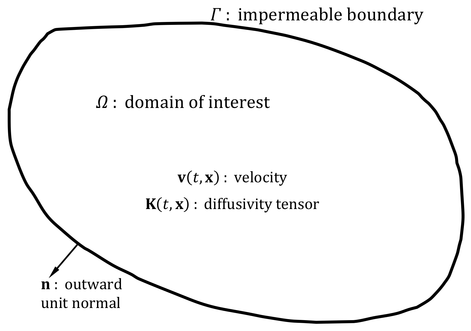
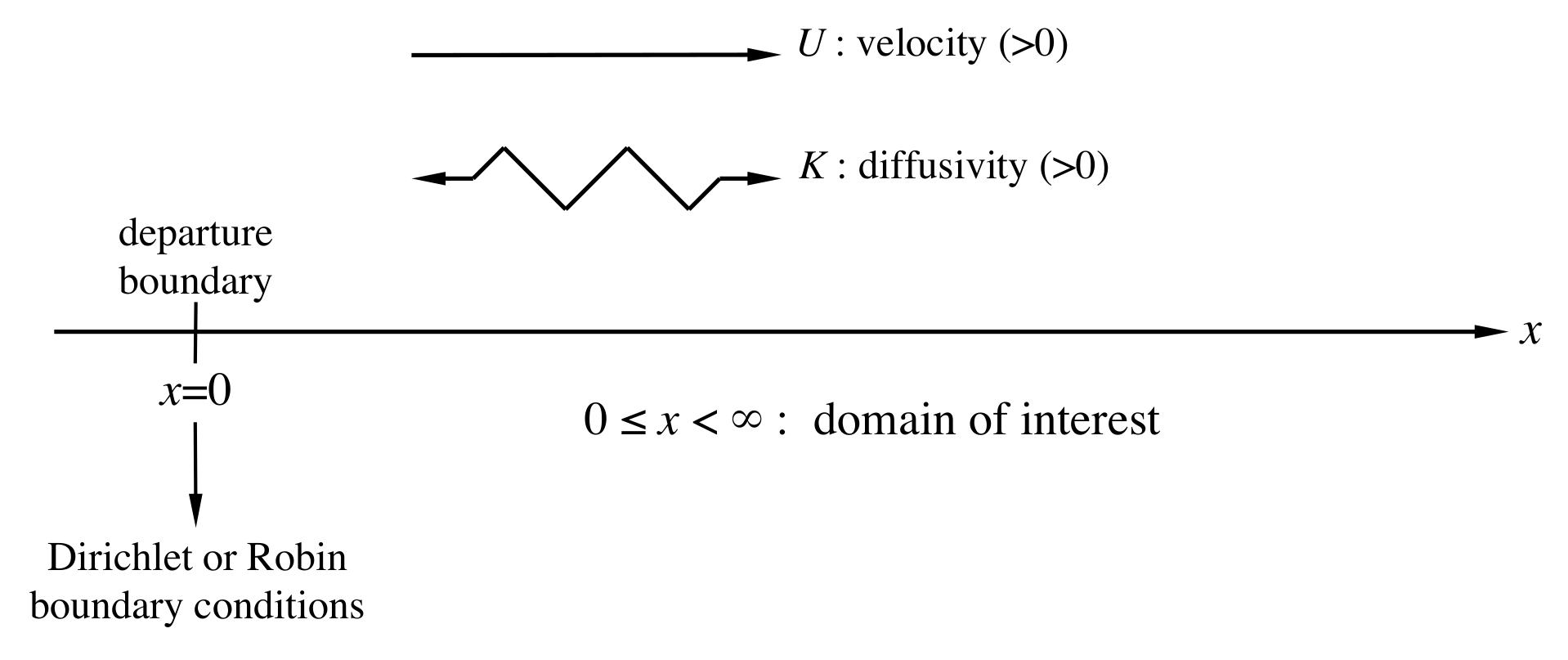
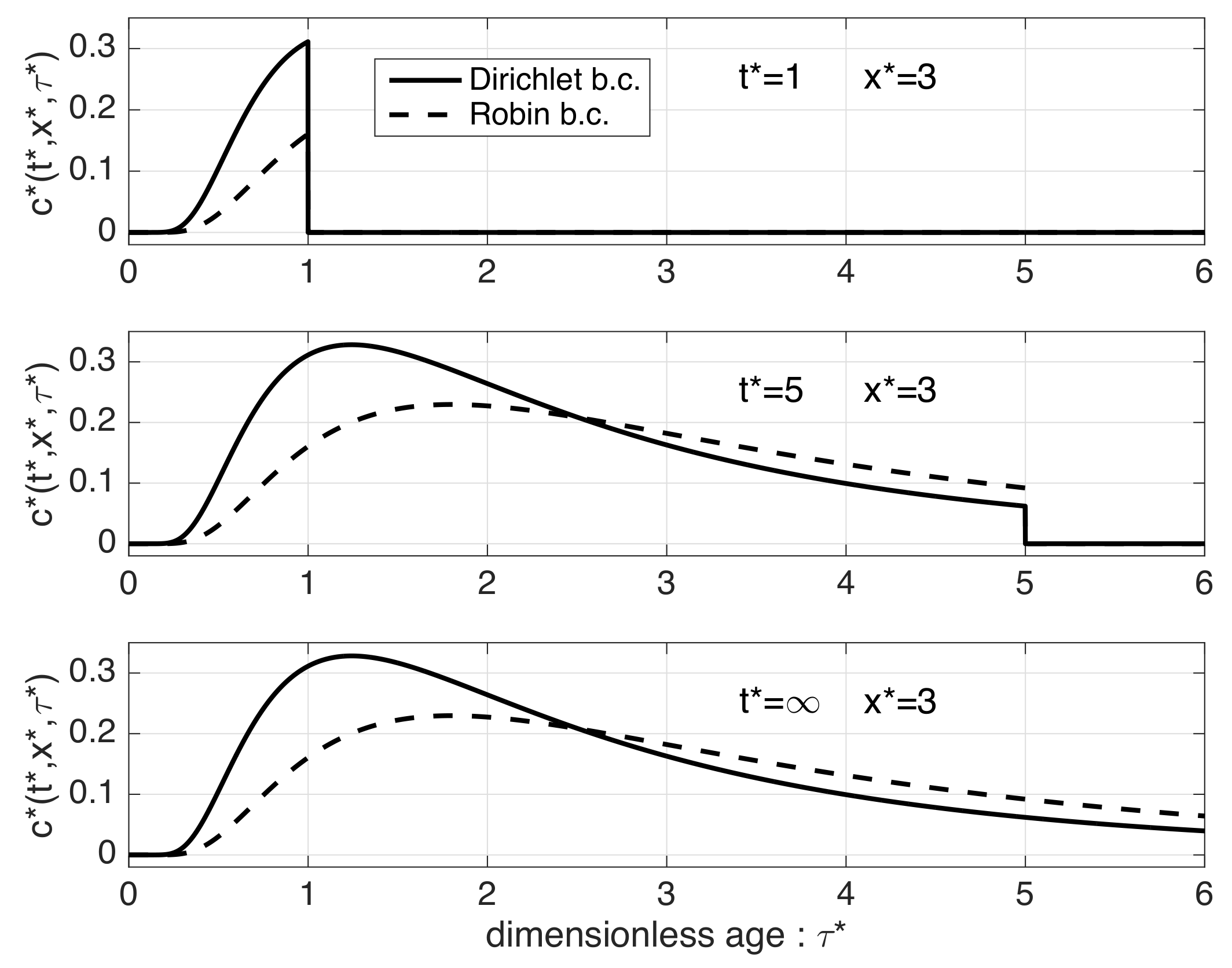
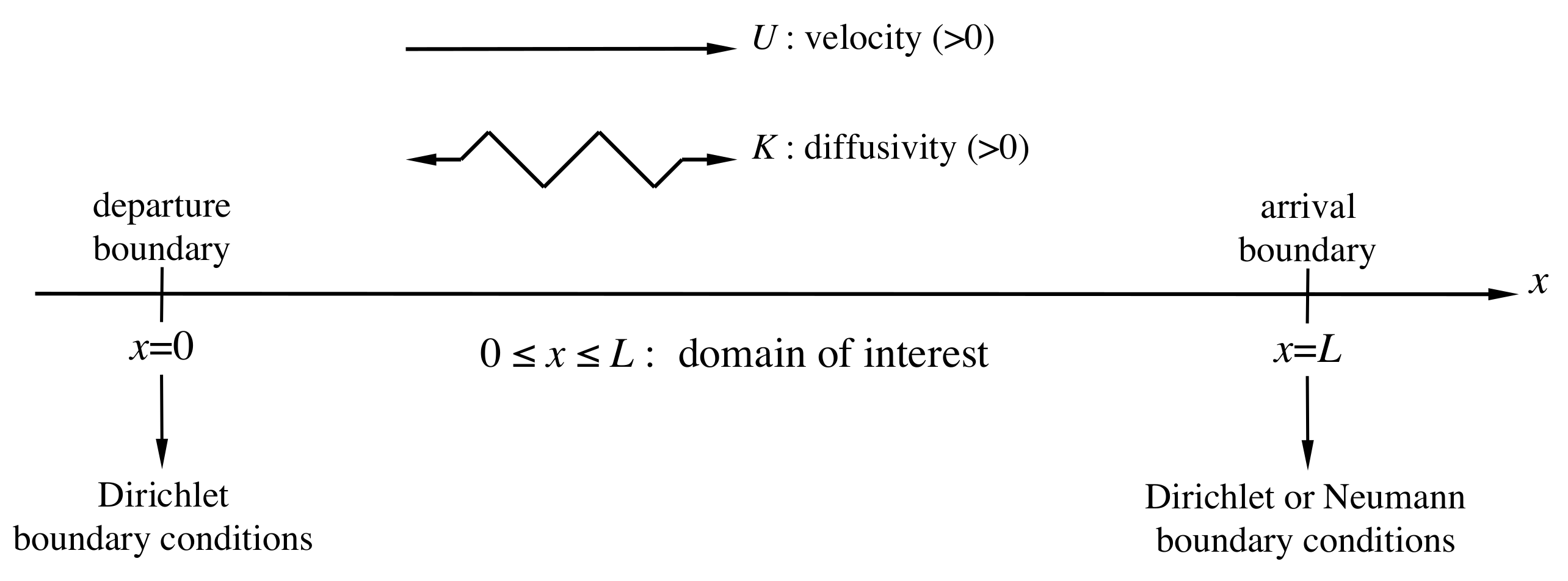
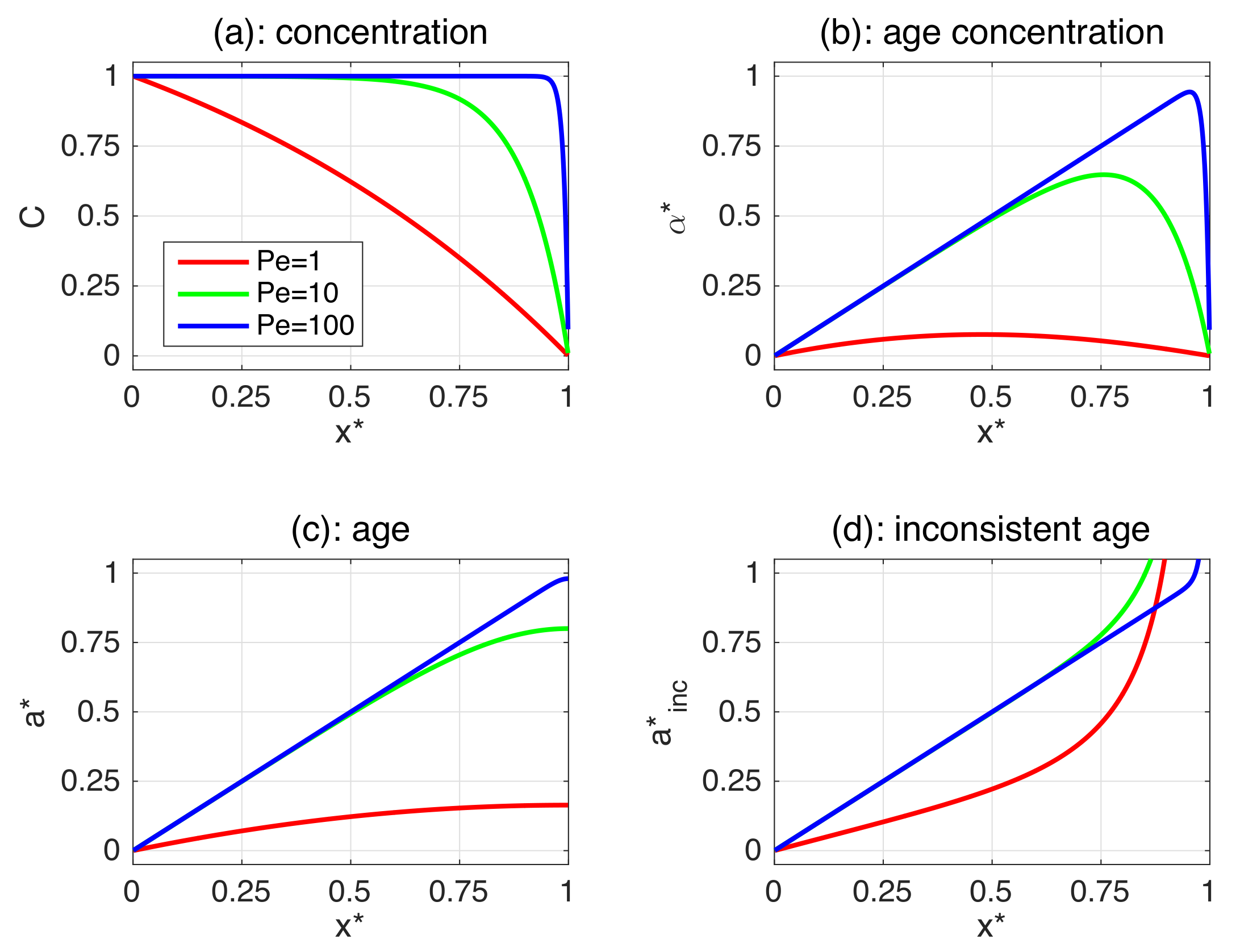
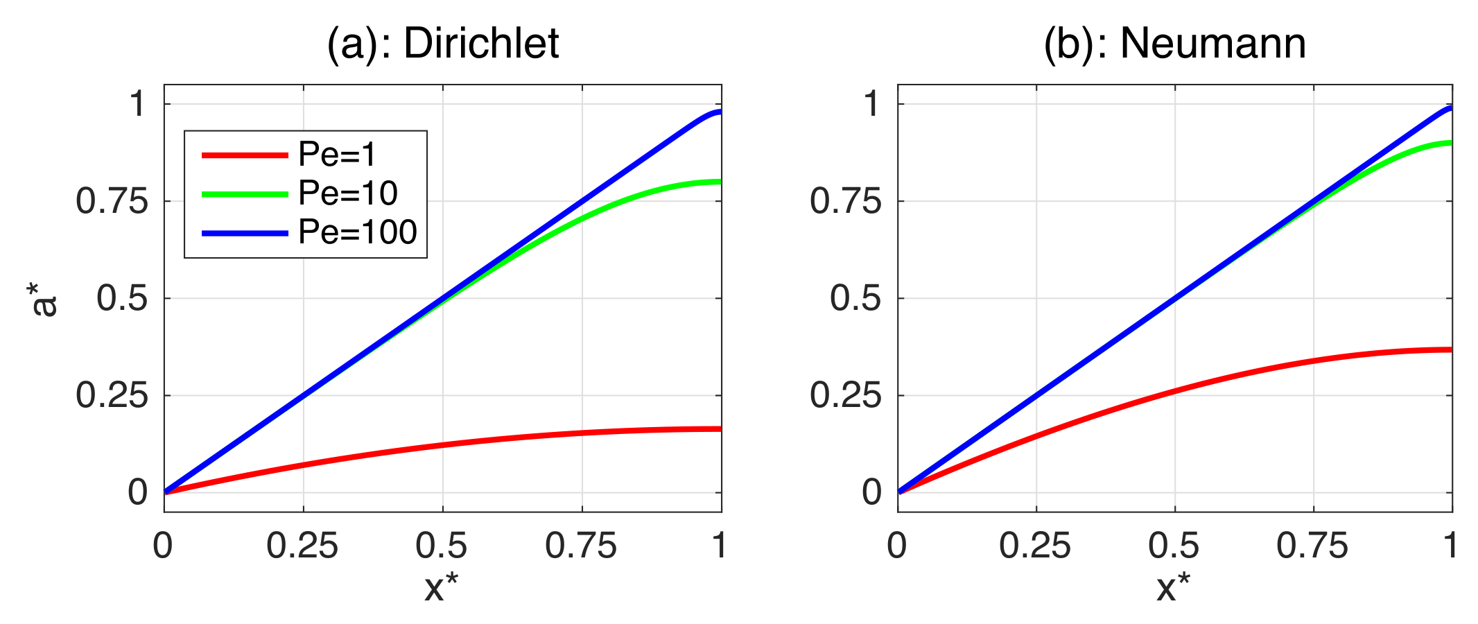
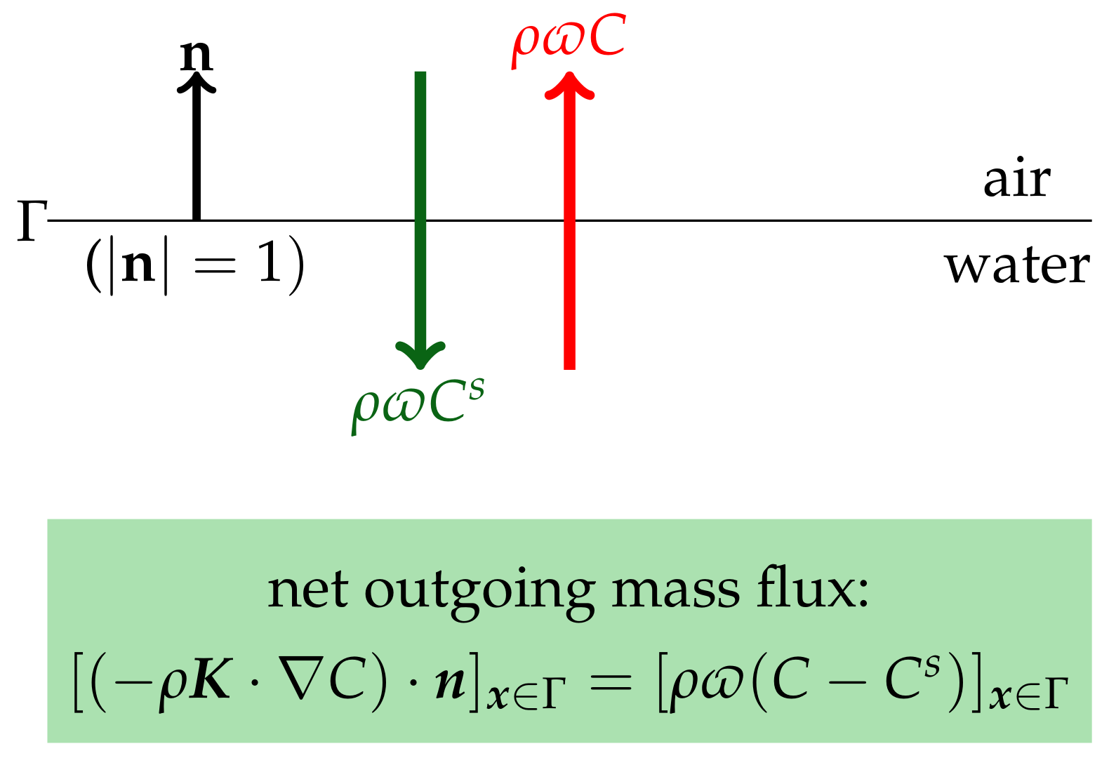
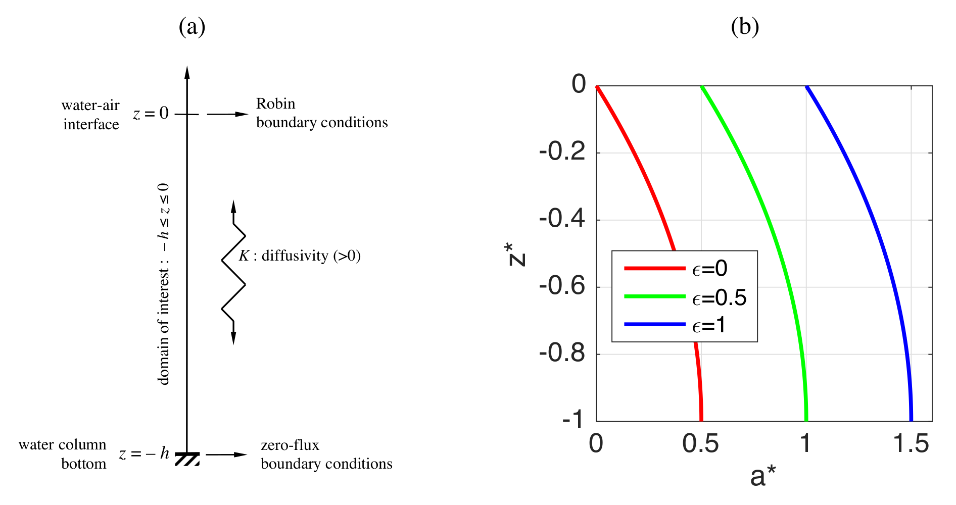
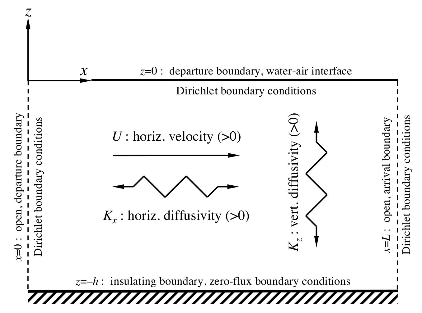
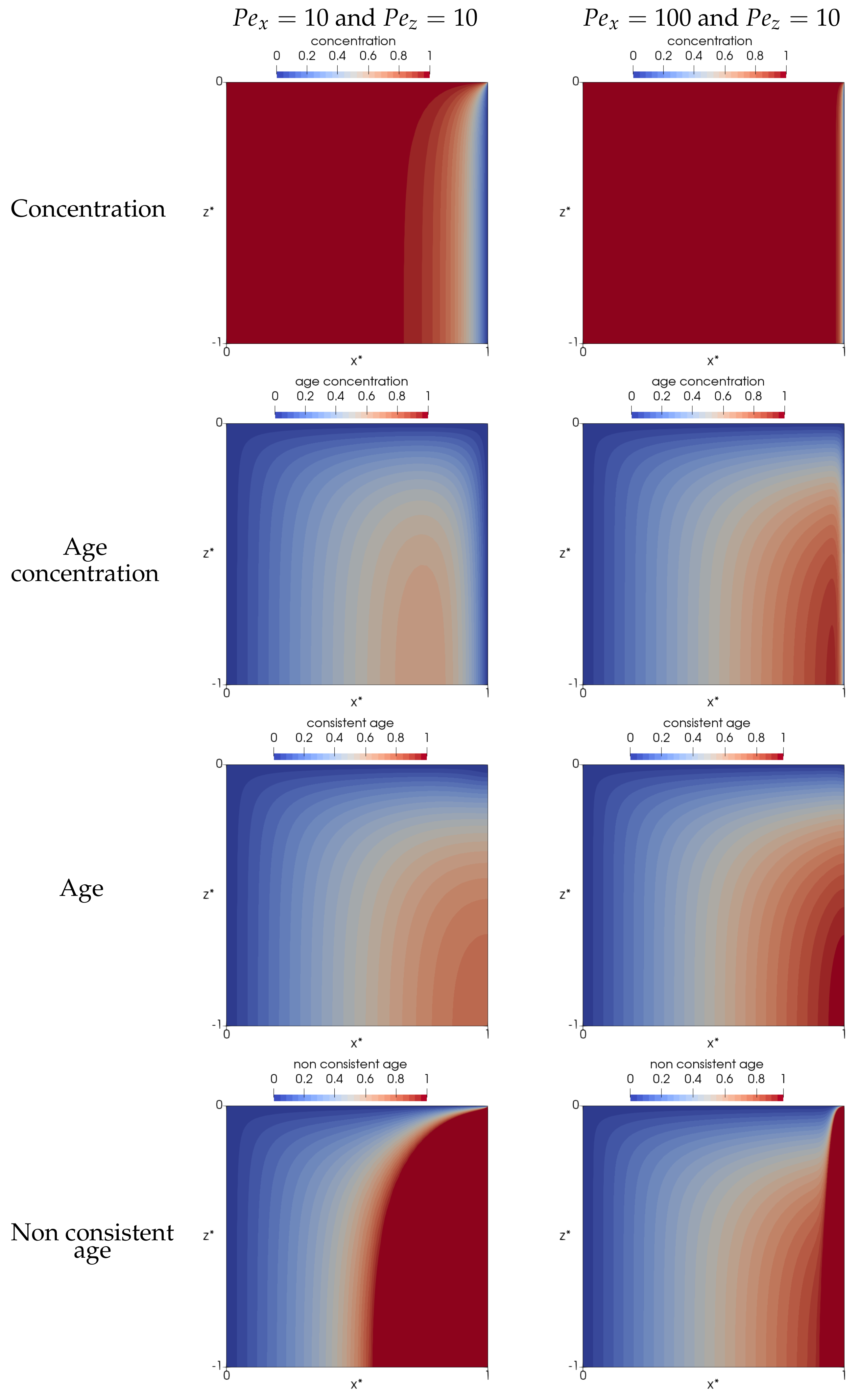
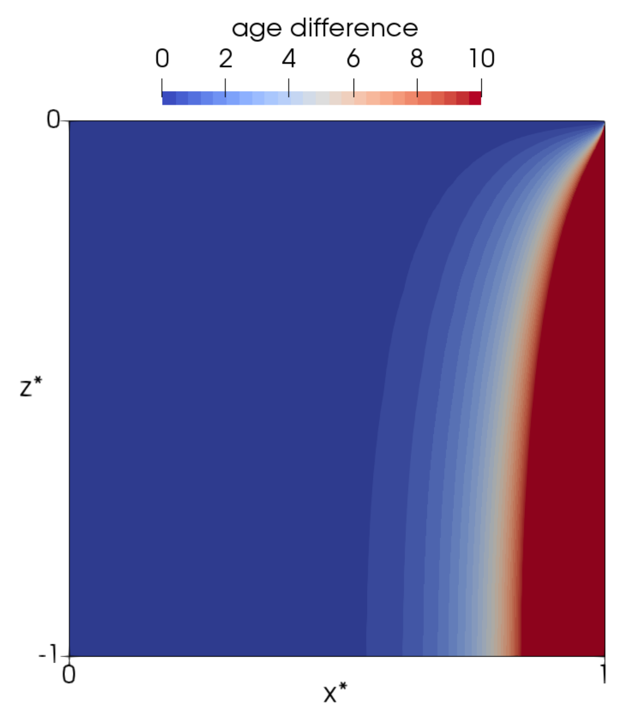
Table 1.
Outgoing and incoming specific fluxes (ratio of a flux to the water density) at the water–air interface for the age distribution function (), the concentration (), and the age concentration (). As for the downward flux, the general expression and two simplified ones are taken into consideration, which consists in assuming that all the incoming gas particles have the same age, (fourth column), and that this age is zero (fifth column).
| Variable | Outgoing (Upward) | Incoming (Downward) Specific Flux | ||
|---|---|---|---|---|
| Specific Flux | General Expression | |||
| age distribution function | ||||
| concentration | ||||
| age concentration | 0 | |||
© 2020 by the authors. Licensee MDPI, Basel, Switzerland. This article is an open access article distributed under the terms and conditions of the Creative Commons Attribution (CC BY) license (http://creativecommons.org/licenses/by/4.0/).
Share and Cite
MDPI and ACS Style
Deleersnijder, E.; Draoui, I.; Lambrechts, J.; Legat, V.; Mouchet, A. Consistent Boundary Conditions for Age Calculations. Water 2020, 12, 1274. https://doi.org/10.3390/w12051274
AMA Style
Deleersnijder E, Draoui I, Lambrechts J, Legat V, Mouchet A. Consistent Boundary Conditions for Age Calculations. Water. 2020; 12(5):1274. https://doi.org/10.3390/w12051274
Chicago/Turabian StyleDeleersnijder, Eric, Insaf Draoui, Jonathan Lambrechts, Vincent Legat, and Anne Mouchet. 2020. "Consistent Boundary Conditions for Age Calculations" Water 12, no. 5: 1274. https://doi.org/10.3390/w12051274
Note that from the first issue of 2016, this journal uses article numbers instead of page numbers. See further details here.