A Self-Contained and Automated Method for Flood Hazard Maps Prediction in Urban Areas
by
 , , , ,
Marco Sinagra
1,* ,
,
Carmelo Nasello
1,
Tullio Tucciarelli
1,
Silvia Barbetta
2 ,
,
Christian Massari
2 and
Tommaso Moramarco
2
1
Department of Engineering, University of Palermo, 90128 Palermo, Italy
2
Research Institute for Hydro-Geological Protection, National Research Council, 06128 Perugia, Italy
*
Author to whom correspondence should be addressed.
Water 2020, 12(5), 1266; https://doi.org/10.3390/w12051266
Submission received: 19 March 2020
/
Revised: 22 April 2020
/
Accepted: 26 April 2020
/
Published: 29 April 2020
(This article belongs to the Special Issue Design of Urban Water Drainage Systems)
Abstract
:Water depths and velocities predicted inside urban areas during severe storms are traditionally the final result of a chain of hydrologic and hydraulic models. The use of a single model embedding all the components of the rainfall–runoff transformation, including the flux concentration in the river network, can reduce the subjectivity and, as a consequence, the final uncertainty of the computed water depths and velocities. In the model construction, a crucial issue is the management of the topographic data. The information given by a Digital Elevation Model (DEM) available on a regular grid, as well as all the other elevation data provided by single points or contour lines, allow the creation of a Triangulated Irregular Network (TIN) based unstructured digital terrain model, which provides the spatial discretization for both the hydraulic and the hydrologic models. The procedure is split into four steps: (1) correction of the elevation z* measured in the nodes of a preliminary network connecting the edges with all the DEM cell centers; (2) the selection of a suitable hydrographic network where at least one edge of each node has a strictly descending elevation, (3) the generation of the computational mesh, whose edges include all the edges of the hydrographic network and also other lines following internal boundaries provided by roads or other infrastructures, and (4) the estimation of the elevation of the nodes of the computational mesh. A suitable rainfall–runoff transformation model is finally applied to each cell of the identified computational mesh. The proposed methodology is applied to the Sovara stream basin, in central Italy, for two flood events—one is used for parameter calibration and the other one for validation purpose. The comparison between the simulated and the observed flooded areas for the validation flood event shows a good reconstruction of the urban flooding.
1. Introduction
The design of hydraulic infrastructures, like sewers or culverts, and the flood hazard maps delineation are based on the prediction of the rainfall–runoff process occurring inside a catchment basin for a given return time period. The traditional approach splits the process into three different steps: (1) the rainfall–runoff transformation, differentiating the total rain into net rain plus infiltration and evaporation, (2) the concentration of the net rain in the hydrographic network and its propagation up to the boundary of the flooded area, (3) the propagation of the fluxes entering the domain of the flooded area.
Different methods are available in the literature to describe the physical processes involved in step (1) [1], which are characterized by the different number of parameters, differentiating their accuracy and possible applications. In step (2), the routing of net rainfall along the river network is generally based on the assumptions of stationarity and linearity [2,3]. This category includes the Instantaneous Unit Hydrograph (IUH), which is based on the hierarchical organization of the river network, as well as on the empirical estimation of the vertically averaged velocity in each point of the basin [4]. In some models, the velocity can be distributed in space as a function of the upstream drainage area, the Manning roughness coefficient in the upstream areas, and the slope of the Digital Elevation Model (DEM) cells [5]. Following this procedure, a single IUH, characteristic of a given catchment area, can be derived assuming the routing velocity constant at each point during the runoff process.
In the last years, many researchers have investigated the idea of solving the flow routing inside the hydrologic network [6]. For the routing process, Looper and Vieux [7] used the one-dimensional Saint Venant Equations (SVE) in their kinematic approximation. The above equations are applied to the cross-sections of the riverbed, directly detected or extracted from a DEM obtained by the LiDAR survey. This allows linking the norm of the flow velocity to the variation of the water depth.
Other researchers tried to compute the propagation of the overland flow inside the basin by solving the two-dimensional SVE on an unstructured triangular mesh. The above equations are usually solved in their complete (or dynamic) formulation [8].
In step (3) the simulation of runoff in flooded areas is conventionally based on one-dimensional (1D) and two-dimensional (2D) numerical models of shallow water (SW) equations [9]. The spread of non-structural solutions for the mitigation of hydraulic risk has motivated research in the last decades to improve the accuracy and the efficiency of 2D SW numerical models, with low computational burden methodologies [10,11,12,13,14], in order to use them in frameworks aimed at real-time flood forecasting.
Even if several advanced hydrological and hydraulic models have been applied for the computation of the whole rainfall–runoff transformation and runoff propagation process, a single tool for the solution of the entire chain linking generation of channel network from orography and hydrological input data with the predicted flooded area is, as far as the authors know, still missing. The procedures available in the literature are typically based on coupling the hydrologic and the hydraulic models in cascade mode, with the need of manipulating the output of the hydrologic model to get the input of the hydraulic one. As an example, Popescu et al. [15] applied an integrated flood simulation system based on the HEC-HMS hydrological model, HEC-RAS for the one-dimensional hydrodynamic model and SOBEK for the two-dimensional (2D). Wang et al. [16] developed a holistic framework for urban flood modeling using different approaches to process the different parameters of a 2D model—DEMs to estimate the topographic elevation, and rainfall to estimate the infiltration parameters. Tanaka et al. [17] proposed an integrated hydrological-hydraulic model employing the 2D local inertial equation for the effective numerical simulation of surface water flows, by designing the model as a cascade of validated hydrological and hydraulic sub-models. Similarly, Grimaldi et al. [18] developed a numerical experiment to quantify the propagation of errors when integrating hydrological and hydraulic models in large basins using a coupled modeling chain consisting of the HBV hydrological model and the hydraulic model LISFLOOD-FP. Nogherotto et al. [19] described an integrated hydrological, and hydraulic approach based on the river discharges estimated through the hydrological model CHyM and on the CA2D hydraulic model to calculate the flow over a digital elevation model. More recently, Aureli et al. [20] solved the complete 2D SW Equations starting from the precipitations and simulating the propagation on structured non-uniform grids.
It is also widely acknowledged that the topographic error occurring at different scales in both the external catchment basin and the flooded urban area is one of the major sources of error, leading to a poor reconstruction of the hydrographic network and, in the flooded area, to a large error in the water depth and flow velocity estimation. Errors may due to a pixel (pit) surrounded by pixels with higher elevations. Removing pits can be done by lifting procedures that, however, may generate flat areas with topographic characteristics such as slopes not realistically represented [21].
A different approach was proposed by other authors [22,23] who combined the “lifting” and the “carving” procedures to limit the changes in the terrain elevation, while Grimaldi et al. [24] applied a sediment transport model after pit removal so that a realistic slope of the terrain surface was finally obtained. All these methods for minimizing topographic errors were developed independently of the context of analysis, such as for a flood hazard assessment.
Based on the above insights, in this study, we proposed a self-contained and automated tool based on three components and aimed to estimate the flood hazard maps in areas that were urbanized and with complex topography. The first component, named Hydronet, generates a Triangulated Irregular Network (TIN) covering all the computational domains (urban and not urban areas) and a set of nodal topographic elevations performing two different tasks—(1) to be a suitable computational mesh for the shallow water hydraulic model, and (2) to form with some of its edges a hydrographic network of previously assigned density. The edges shared with the hydrographic network are also flow paths in the hydraulic model; therefore, this peculiarity allows a good reconstruction of the flow field even with a simple planar approximation of the topography on the two sides of each edge, without the need of adapting the computational mesh and the hydraulic model parameters to the computed hydrographic network geometry. The method leverages topographical data coming from a digital terrain model, integrated by other available information, and leads to a TIN, also taking hydraulic infrastructure elevations into account. The second component is a simple hydrologic model able to represent the distribution of rainfall excess starting from the observed precipitation or forecasted by weather models. The third component is a 2D hydraulic model aimed to efficiently estimate the flooded area using the same spatial discretization of the TIN model, leveraging the heterogeneity of the computational mesh density inside the urban and the upstream basin area. The proposed tool requires as input the DEM of a basin, additional topographic information representing hydraulic singularities as culverts, levees and bridges, as well as observed/forecasted precipitation, and is able to provide the flood maps automatically. The proposed tool has the peculiarity to be self-contained and might be an alternative to complex frameworks where data and parameter-intensive models are applied separately for flood risk analysis and management. The urban area of the Pistrino town in the Upper Tiber River basin, in central Italy, is used as a case study.
2. Operational Method for Flooded Areas Forecasting
The proposed operational method for flooded area forecasting is based on three main components.
The first component is a self-contained procedure for the spatial discretization of the entire basin, named the Hydronet. This component computes a TIN irregular mesh, serving at the same time as the topographic model and support for the spatial discretization of the governing flow and momentum equations. The procedure for the TIN computational mesh identification is based on five steps (see Section 2.1) that, starting from DEM, make a correction to the topographical data by removing sinks and peaks, identifying a hydrographic network through which the runoff is formed and routed, and finally include singularities given by infrastructures (like levees, roads, railways, and culverts).
The second component is a simple hydrological model based on the Soil Conservation Service Curve Number (SCS-CN) method which allows to easily estimate the rainfall excess and, from that, the runoff according to the 2D topographic model identified by the Hydronet. This component can be easily replaced by a more complex rainfall–runoff transformation model if the data required for its calibration are available.
The third component is the routing 2D WEC-Flood model, which solves the diffusive form of the Saint Venant Equations using the same spatial discretization provided by the TIN computed by the first Hydronet component.
2.1. Hydronet Algorithm
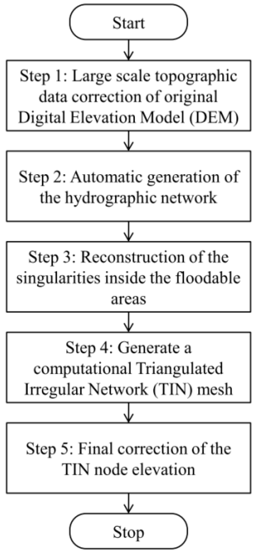
The Hydronet algorithm is split into five steps, starting from the DEM data of a rectangular area, including the catchment basin and other topographic information, usually available in the urban area (Figure 1).
Step 1
The original DEM cell elevations, assumed to hold in cell centers are corrected in order to guarantee a minimum negative slope (i.e., descending) in at least one of the eight directions connecting each cell with the neighboring ones. The mesh given by the connection of each cell center with all the surrounding ones is called “preliminary mesh”.
Step 2
The hydrographic network of the basin is generated by discarding most of the edges of the “preliminary mesh”, including the edges connecting the cells with a very small upper drainage area.
Step 3
The singularities inside the flood-prone areas are reconstructed by adding to the hydrographic network other piecewise linear curves, where the topographic elevation is known (like roads or railway lines).
Step 4
A computational TIN mesh is generated adopting the edges of the hydrographic network and the other curves introduced during Step 3 as internal boundary sides, linking all the centers of the cells not discarded in Step 2, as well as the other elevation points added in Step 3. All the points linked by the internal boundary sides are nodes of the mesh. The resulting TIN mesh density is typically very highly close to internal boundaries and much lower in most of the internal nodes. The node elevations are interpolated from the cell elevations and the elevation of the curves imported during Step 3.
Step 5
The final correction of the TIN node elevations is carried out to avoid local minima given by the interpolation procedure.
The above procedure is shown in the flowchart of Figure 1. The single steps are explained in details in what follows.
2.1.1. Large-Scale Topographic Data Correction (Step 1)
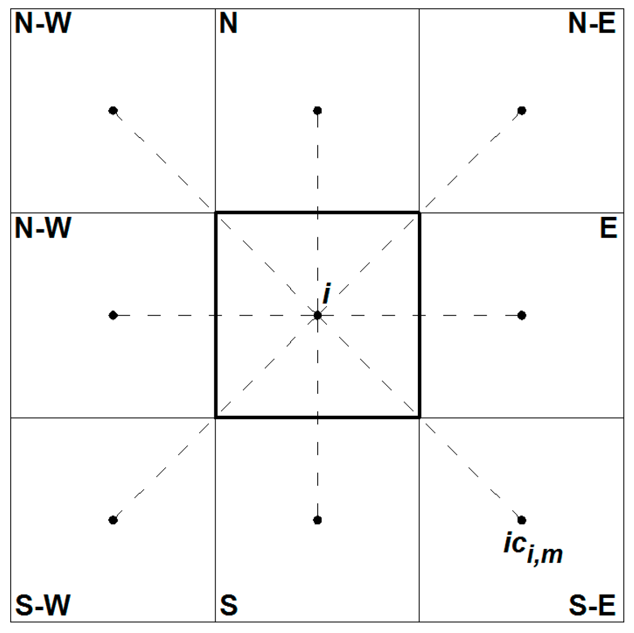
The DEM correction is carried out through the approximated solution of the so-called “constrained minimization” (CM) problem, where the objective function is the sum of the square difference between the estimated elevations in the center of each cell, zcm, and the measured mean values, z*. The outlet of cell of the basin, with the minimum elevation, is called the “root cell”. The sought-after solution is constrained by the existence, for each cell different by the “root cell”, of at least one companion cell among the neighboring ones, with a strictly smaller elevation. Figure 2 shows the eight neighbor cells surrounding a generic cell inside the basin and the corresponding directions. We call this zcm solution the “optimal” solution of the CM problem. The mathematical statement of the minimization problem is described in details in Appendix A.
The CM problem is a mixed real-integer non-convex minimization problem with millions (or even billion) of variables, and several local minima greater than the global one, quite hard to be solved with standard computational tools. We show in the following, that a good sub-optimal feasible solution, named zc, can be found as a combination of two auxiliary solutions, each one being a local minimum satisfying the required constraints, called “upper” and “lower” solutions. The auxiliary “upper” solution (zu) has all the computed elevations greater than or equal to the measured z*, while the auxiliary “lower” solution (zl) has all the computed elevations smaller than or equal to the measured z*. The two solutions differ from z* only in small areas not connected to each other, and can be easily combined to get a very good final approximation of the optimal solution.
Let us say that iout(i) is the cell, among the neighbors of cell i, where zu(iout(i)) satisfies the required constraint with respect to zu(i), with the minimum (most negative) slope along the corresponding direction. The identified auxiliary “upper” solution of the CM problem can be seen as a tree of cells linked by edges, with the root in the outlet cell of the catchment basin. The ensemble of all the edges linking the center of the cells i and iout(i) represents the hydrographic network with the maximum possible density inside the basin.
Before starting the correction procedure, the cells on the contour of the catchment basin are selected. All the cells outside the catchment boundary are not included in the correction procedure.
Computation of the “Upper” Solution
The zu “upper” solution is a local minimum of the CM problem, where at least one drainage direction with a negative slope exists for each cell, excluding the outlet one, and all the corrected elevations are higher than or equal to the measured one. This solution has already been proposed by many authors as the final correction of the DEM values, like in ref. [12] or ref. [25]. A simple procedure for quick computation of the “upper” solution is described in Appendix A.
The “upper” solution is the same as the “filling up” methods, where it is found by increasing all the artificial minimum elevation points. The “upper” solution is often a good feasible sub-optimal solution of the CM problem, but it always overestimates the optimal one, with an artificial flat area covering each artificial minimum. If a positive error is given in the elevation datum of a cell i inside an impluvium, all the upstream part of the impluvium will be artificially raised, up to the elevation of cell i. To avoid this problem, many methods like ref. [22] or ref. [24] try to “breach” the artificial “dam” created by the positive errors or to simulate the natural erosion process for the removal of the artificial deposit.
On the other hand, if we assume that no bias is present in the elevation measurement and other information on the soil parameters are missing, correction given by a solution, as close as possible to the optimal solution of the CM problem, is likely to be the most appropriate one. In the following correction we try to find a better sub-optimal feasible solution of the same problem.
Computation of the “Lower” Solution and of the Final One
To improve the sub-optimal solution of the CM problem given by the zu “upper” one, we search a “lower” solution zl with corrected elevations always smaller than the measured ones. To identify the “lower” solution, we maintain a negative (i.e., descending) sign of the slope in the direction from cell i to the cell iout(i), previously computed in the search of the “upper” solution, for all the cells i except the outlet one. Say leaves the cells that are not drained by any other cell, and do not match the cell iout(i) of any cell i inside the basin. Starting from each leaf cell the procedure, described in details in Appendix B, computes the auxiliary solution zl by moving along all the branches defined by the directions i-iout(i) found in the previous step and by setting the cell elevations at the maximum elevation compatible with (1) a descending slope along the branch and (2) the condition . Observe that in the “lower” solution the elevation of the outlet cell can be lower than the DEM measured one.
The “lower” zl auxiliary solution is also a good approximation of the measured DEM elevation z* and, very important, both the “lower” and the ”upper” auxiliary solutions match the DEM elevation in the major part of the catchment area. Say A the subset of the basin cells where the “upper” solution is strictly greater than the “lower” solution. Using good quality DEM data, the size of A, where zui or zli is not equal to , is of the order of 1% of all the cells or even less. Moreover, these cells are clustered inside many small areas disconnected from each other. Say Aj the jth sub-set of the cells of A connected to each other. The final solution is found by minimizing the square difference between the elevations measured in each sub-set Aj and the elevations obtained as a linear combination of the “upper” and “lower” solutions in the same sub-set. The weight of the linear combination is the same for all the cells of the sub-set; therefore, the properties of both the “lower” and “upper” solutions are saved in the final one, named zc. See a detailed description of the algorithm in Appendix C.
The entire process is particularly fast if a proper ordering of the cell elevation correction is carried out. For the Sovara case study, with 3.8 × 10⁶ cells, the stationarity is achieved in about 10 min (including I/O operations) using a single core of Intel(R) i7-4770 CPU 3.4 GHz.
2.1.2. Automatic Generation of the Hydrographic Network and of the TIN Hydraulic Computational Mesh (Steps 2–4)
Correction of elevation z* (Step 1) is the basis for the computation of the hydrographic network. This network can be thought of as the ensemble of the segments connecting the centers of cells i, iout(i). These segments can only have four possible directions—the x-direction, the y-direction, and the two diagonal directions. The use of all the i–iout(i) segments would lead to a bad representation of the basin and, most importantly, it would not help the generation of a TIN as support for the runoff propagation model. In order to reduce the complexity of the hydrographic network, we need to order all the cells inside the basin according to their drainage area. Our final hydrographic network is the network resulting from the i–iout(i) segments connecting all the cells characterized by a drainage area/basin area ratio greater than a minimum value, named threshold ratio Sill.
The use of a small threshold ratio, even close to 1%, provides a dramatic reduction of the number of segments i–iout(i) considered for the representation of the hydrographic network.
The computed hydrographic network represents an optimal basis for the generation of a TIN to be used as spatial discretization in the shallow water hydraulic model. In the sought-after TIN, all the segments of the hydrographic network are set as internal boundaries and overlap triangular edges. All the segments have a descending slope in the i–iout(i) direction; hence, artificial obstructions (like artificial topographic minima or river “cutting edges”) will not be met by the simulated channel flows. Most importantly, with a suitable setting of the mesh-generator parameters, it is possible to get a strong heterogeneous TIN mesh density, decreasing along with the distance from the internal boundaries given by the sides of the hydrographic network. This leads, in the final 2D hydraulic model, to a massive reduction of the required memory storage and computational time.
The hydrographic network is not the only internal force available for the generation of the computational grid. Actually, in flood-prone areas where urban areas exist, anthropic elements, such as roads or urban river embankments can have a strong impact on the flow directions. The elevation trend of the top of these elements can be reconstructed by means of three-dimensional lines assuming a linear variation of the elevation along each segment of the line. Also, these segments are added to the sides of the hydrographic network to provide the internal boundaries for the mesh generation.
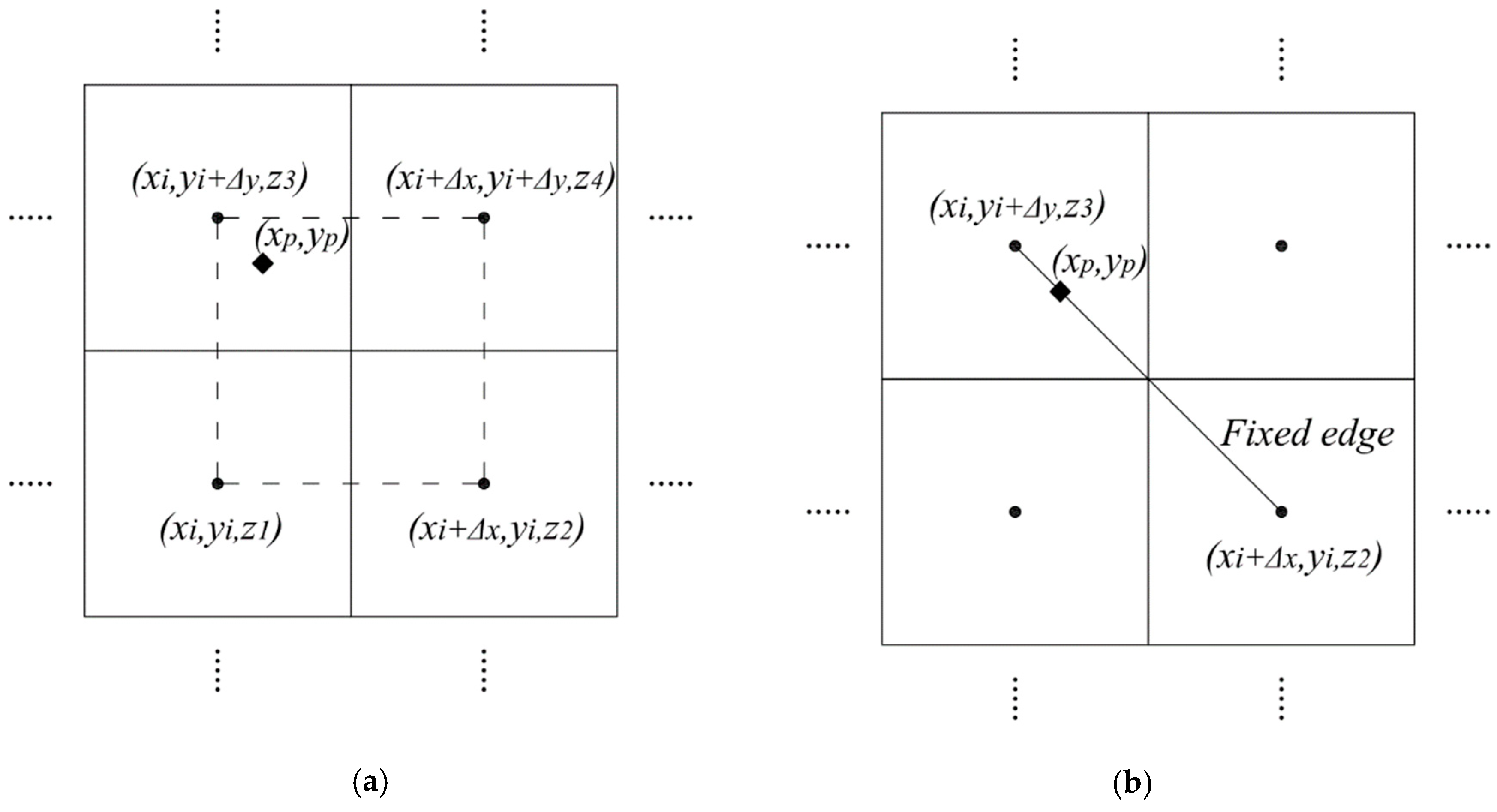
If we call zp the vector of the TIN node elevations, which is computed by interpolating the elevations of the cell centers and the points included in the three-dimensional lines. In order to improve the estimated elevation of the new nodes generated inside the TIN, a bilinear approximation is adopted inside the rectangular area within the centers of four neighboring cells of the original DEM model sharing a common point (Figure 3a). If the rectangular area has one edge of the hydrographic network along its diagonal direction, the interpolation is shifted to a triangular linear interpolation, with the diagonal side in the same direction of the edge of the hydrographic network (Figure 3b).
2.1.3. Computation of the Final Node Elevation (Step 5)
Even if no more local minima exist in the corrected cell center elevations, the interpolated zp elevations could show artificial minima due to the manual management of the topographic information or the possible large extension of some triangle sides. To avoid this effect, an “upper” solution of the ground elevation of the TIN nodes is found, named z, according to the algorithm described in Appendix D.
In the computational procedure, the elevation of all the nodes aligned on the sides of the hydrographic network is initialized with the values linearly interpolated from the elevation of the connected cell centers. The adopted correction procedure does not change the elevation of these nodes because it saves the minimum slope condition of all the nodes of the network, and all the nodes along the sides of the hydrographic network start with a minimum negative slope.
In the computational TIN, all the edges of the network are either new sides of triangles, or are the original sides of the internal boundaries, split into smaller edges aligned in the same direction. The mesh will have the maximum density close to the hydrographic network, but the triangular shape of the elements allows a strong reduction of the mesh density in areas with higher slope. The sequence of the computed elevation vectors is summarized in Table 1.
2.2. Runoff Model
According to the 1D vertical infiltration approximation, several models can be used for the net rainfall computation. In the following, the Soil Conservation Service-Curve Number (SCS-CN) method is used [26] for its simplicity and input data parsimony. In each cell, at every time step, the net rainfall is computed from the total known rainfall P, the initial abstraction ratio λ and the retention parameter S as:
The value of the S parameter is calculated as:
The values of CN are known in the literature for various land covers and soil textures, within a maximum slope of about 5% [27]. Steep slopes decrease infiltration, and several researchers have proposed empirical formulae for adjusting the corresponding CN-values [28]. The initial abstraction ratio λ has been originally proposed equal to 0.20 [26], but recent studies [11,29] suggest lower values.
The rainfall intensity is assumed constant around each rain meter, inside the polytope defined by the Thiessen polygon. Due to the rain heterogeneity, the average value for a given time return period has to be changed according to a reduction factor ARF such as that proposed by Moisello and Papiri [30]. ARF is a function of the actual areas of the Thiessen polygon and of the mean duration of every single storm during the simulated event:
where A (km2) is the extension of the Thiessen polygon and d (hours) is the duration of every single storm. In the implemented model, the measured rainfall intensity is multiplied by the ARF factor.
2.3. Routing Model
The hydraulic model used in the proposed methodology for the runoff routing is an integrated 1D–2D model, named WEC-Flood, already introduced by some authors of this paper [13,14,31]. The model adopts the diffusive wave approximation of the Saint Venant Equations to obtain a system of differential equations(Equations (4) and (5)), in the 1D and 2D computational domains, respectively [14]. Equations (4) and (5) are solved in the piezometric head unknown, H:
where t is the time, s is the 1D spatial coordinate measured along the flow direction in the main channel, σ is the transverse 1D cross-sectional flow area, q is the 1D flow rate, B is the channel width, Q is the source term (i.e., the inlet flow rate per unit length), J is the friction slope, h is the water depth, α is the bottom slope, n is the Manning roughness coefficient, and x and y are the Cartesian directions.
To solve Equations (4) and (5), an unstructured hybrid mesh is used. 1D channels are discretized using quadrilateral elements, with one couple of opposite edges overlapping the trace of two river sections and the other couple connecting their ends. The trace of each river section is extended up to the minimum topographic elevation where 1D flow conditions are expected. The 2D computational domain is given by the whole area of the catchment basin and is discretized by triangular elements satisfying the Generalized Delaunay conditions [13]. The use of the diffusive model in the 2D domain, instead of the fully dynamic one, is mainly motivated by the smaller sensitivity of the computed water depth with respect to the topographic error [13].
The model is solved in the context of the MAST (MArching in Space and Time) approach [32], where the solution at the end of each time step is sought after through a fractional time step procedure, splitting the original problem (4) and (5) in a prediction plus a correction sub-problem.
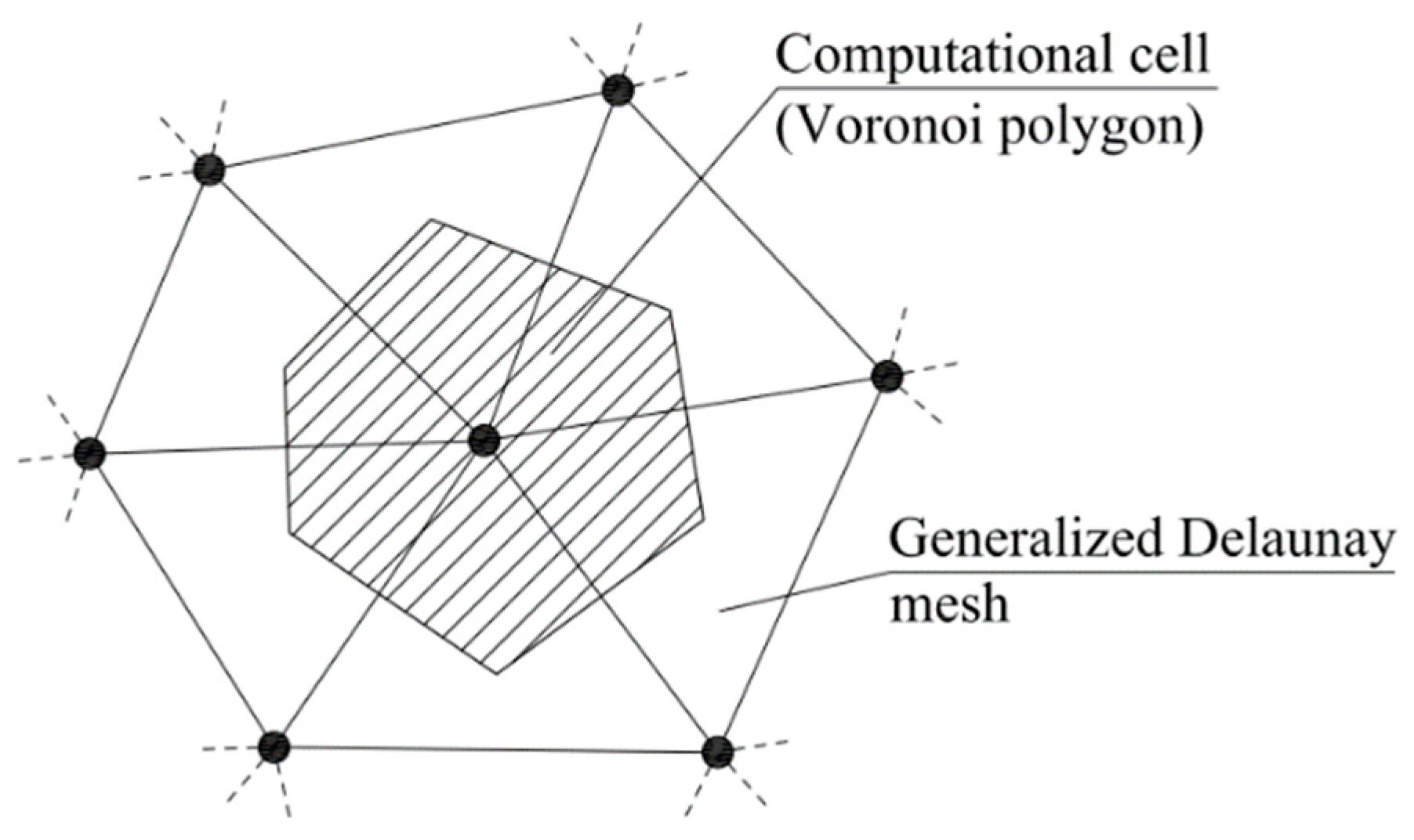
The source term Q in the right-hand side of Equation (5) is given by the net rainfall intensity, which is integrated over the whole cell area (Figure 4). The assumption is made that the infiltration below the ground surface is given only by the direct rainfall and no other infiltration is provided by the overland flow.
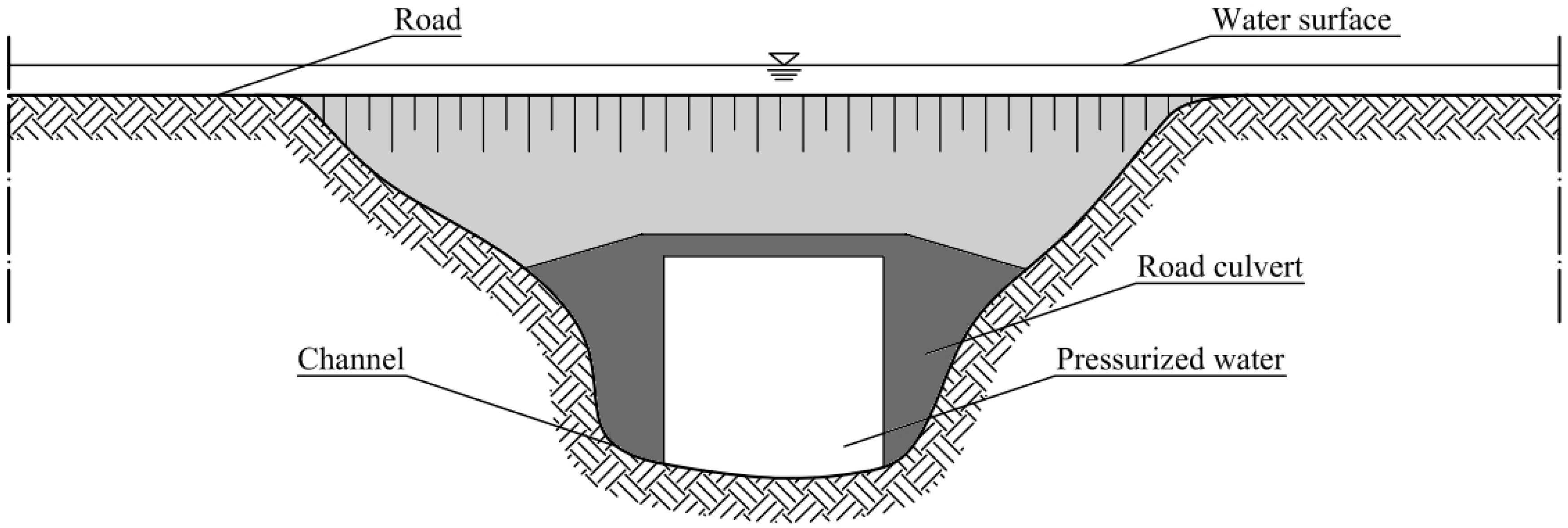
In urban areas, underground hydraulic channels (named culverts) are very often present and allow an impluvium to cross the urban area. During intense rainfall events, when the peak flow overcomes the flow capacity of the culvert, the upstream flow is split into two parts. The first part is the discharge occurring in the pressurized culvert; the second part is the shallow water flow occurring over the ground covering the culvert and also going into the lateral floodplains (Figure 5). Appendix E describes a simple way to include these structures in the hydraulic model.
3. Case Study and Model Setup
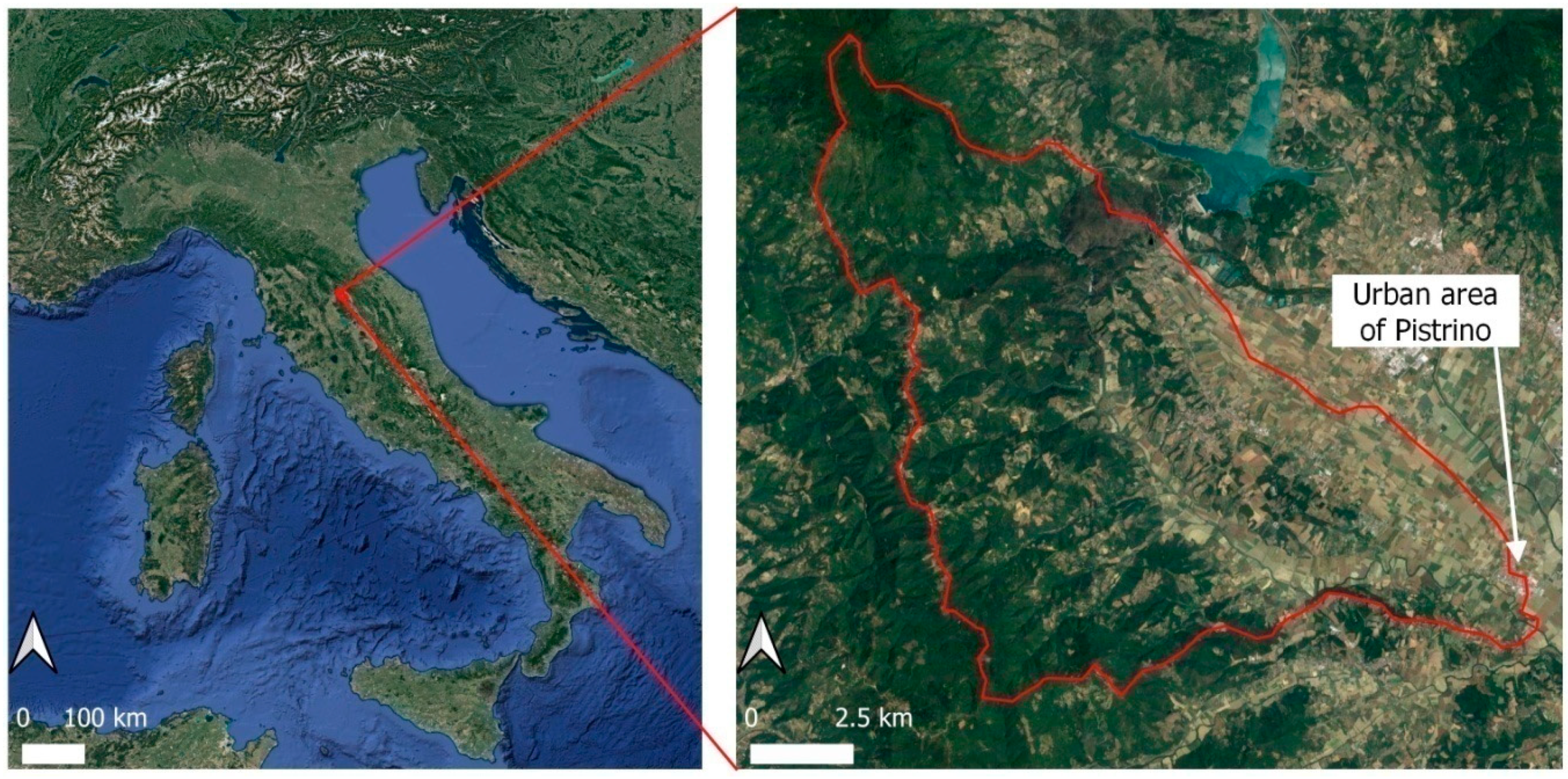
The proposed hydrologic-hydraulic coupled model is applied to a small catchment located in central Italy (Figure 6), the Sovara stream basin with a drainage area of about 134 km2. In the downstream part of the basin, the urban area of Pistrino, on the left of the Sovara stream, is subject to flooding phenomena during intense rainfall events.
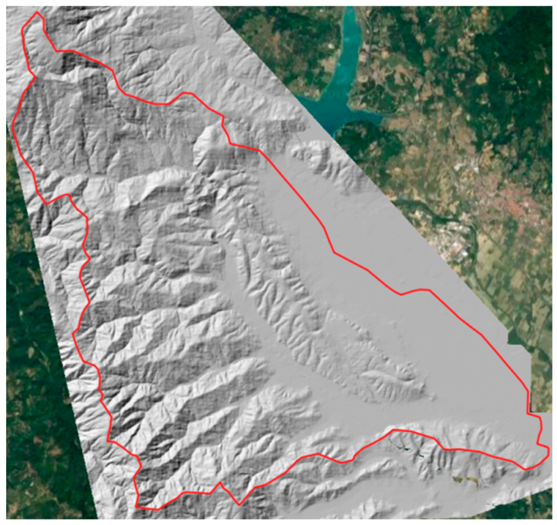
The topography of the whole basin is reconstructed from a 10 m × 10 m DEM covering the total area (Figure 7). In order to estimate the elevation of the river banks and of the main road embankments in the urban area, a 1 m × 1 m DEM is also used.
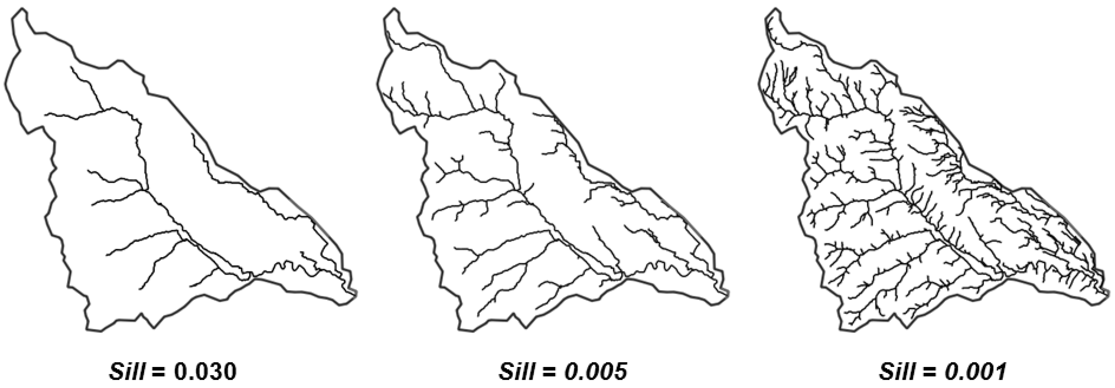
Figure 8 shows the hydrographic network obtained with different Sill values, using the procedure described in Section 2.1.
Obviously, a Sill value reduction leads to an increment of the number of elements in the computational mesh both in the urban and in the upstream basin areas. In the case study, a threshold ratio equal to 0.017 is deemed to be low enough to generate a good approximation of the hydrographic network.
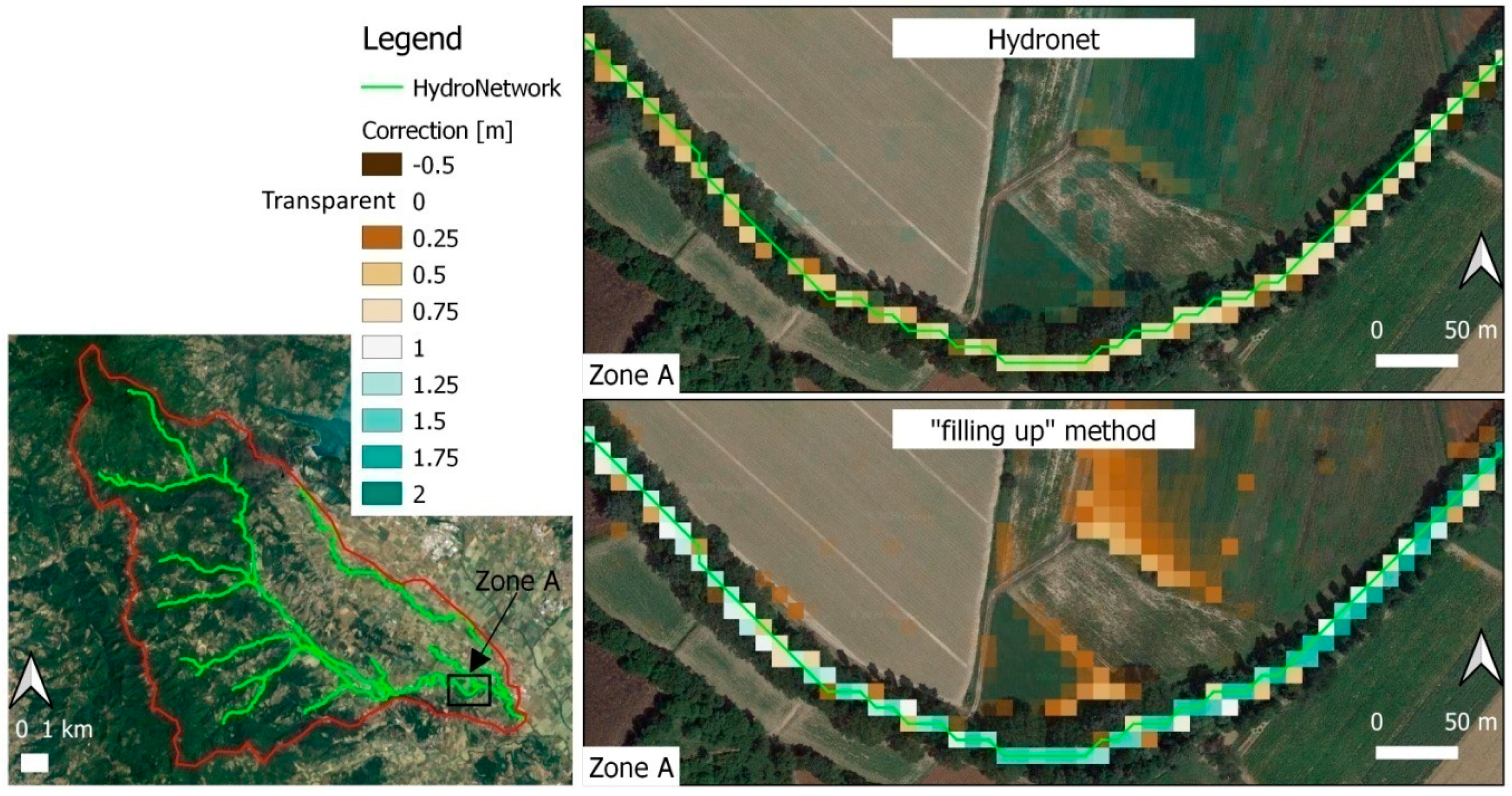
The Hydronet algorithm provides a residual correction error of the DEM cell elevation, expressed by Equation (A1), equal to 4.67 × 10⁻². In the case of correction by the “filling up” methods only, the same error is equal to 8.17 × 10⁻², that is almost twice the one obtained by the Hydronet. Figure 9 shows how the correction by the “filling up” methods can provide a significant local overestimation of the bottom elevation inside channels, with an artificial flood prediction in the neighboring areas. In the same figure, observe that along a single channel of the case study, the “filling up” method raises the bottom elevation up to 2 m, for a maximum length of about 900 m. On the contrary, the maximum correction carried out in the same channel by the Hydronet is restricted to 0.75 m.
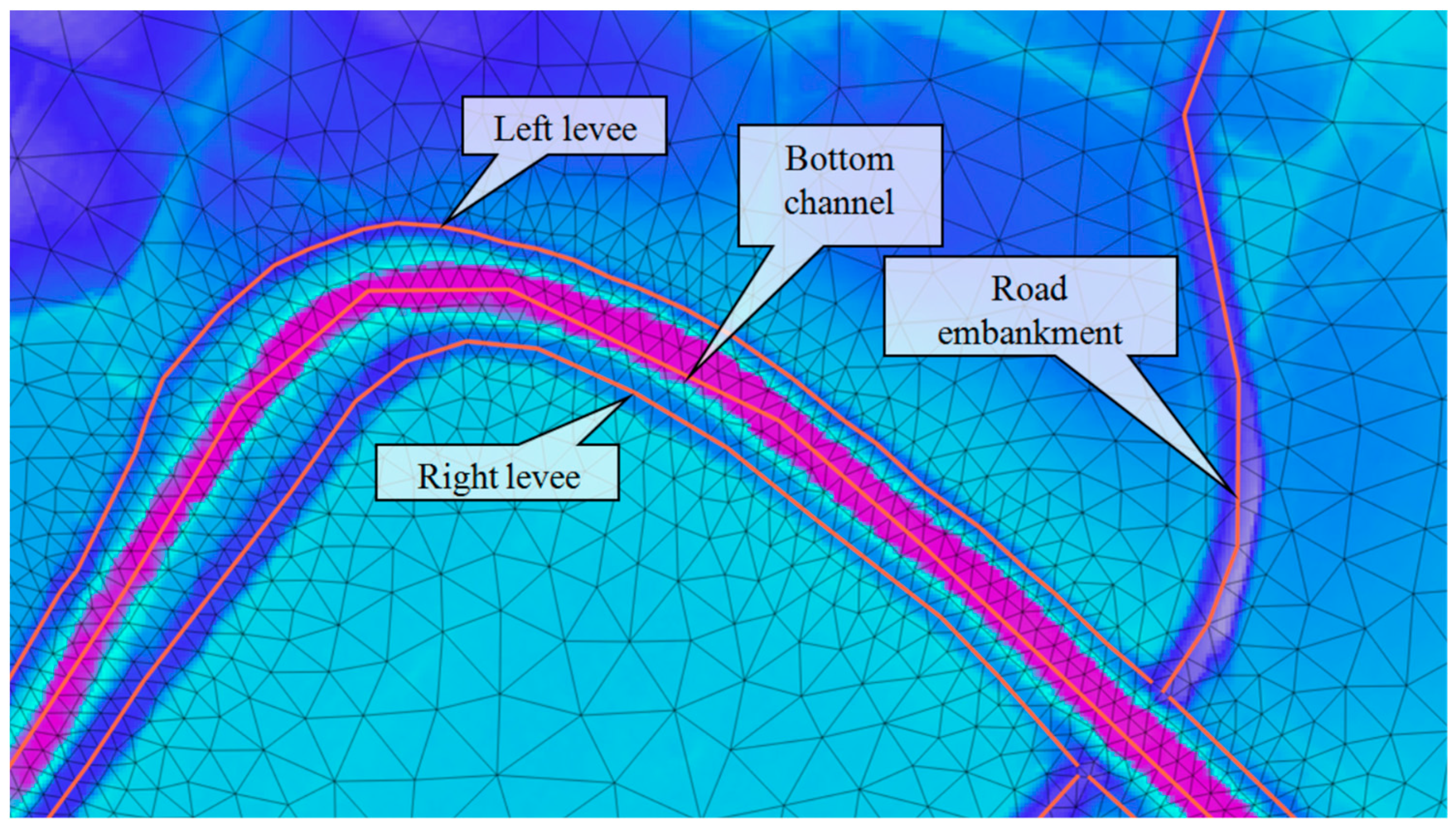
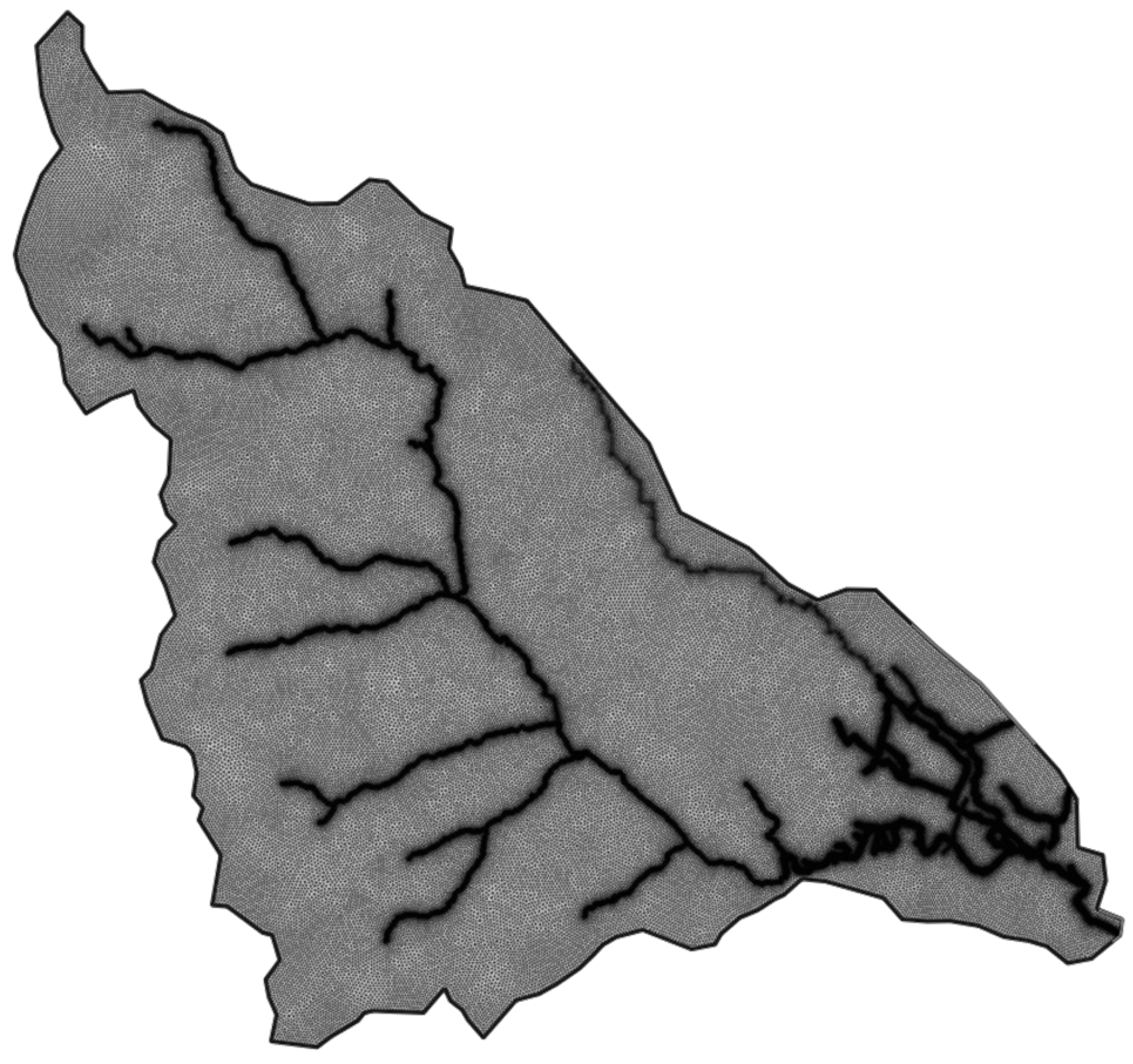
In addition to the generated hydrographic network, the land elevation in the urban area has been improved by inserting 3D lines along the river levees and road embankments, manually reconstructed. The resulting mean length of the triangle sides is between 10 m and 200 m in the basin area, and between 2 m and 5 m around the topographic singularities of the urban area (Figure 10). A computational mesh of 383,940 elements and 192,636 nodes has been finally generated (Figure 11).
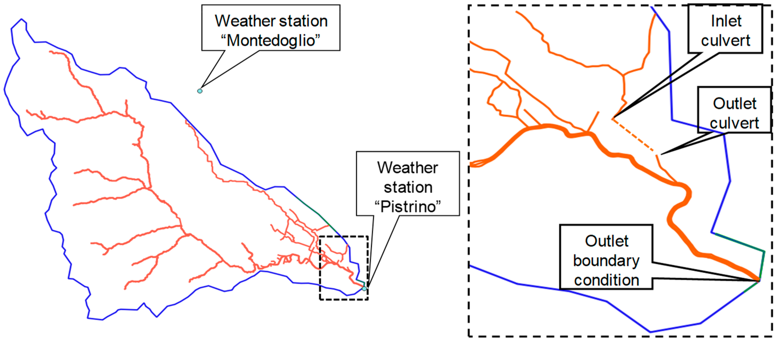
One gauged hydrometric station is available at the outlet section, as well as two rain gauges, named the “Montedoglio” and “Pistrino”. The “Montedoglio” rain gauge is located immediately out of the basin boundary (Figure 12).
A culvert of about 520 m length is located in the urban area close to the gauged section (Figure 12). This structure is very important because it delivers discharges concentrated during ordinary storms below the residential area, with a carrying capacity insufficient in the case of extreme events. To include it in the model, the two mesh nodes next to the inlet and to the outlet of the culvert have been connected with 1D channel edges, according to the procedure described in Appendix E.
4. Results
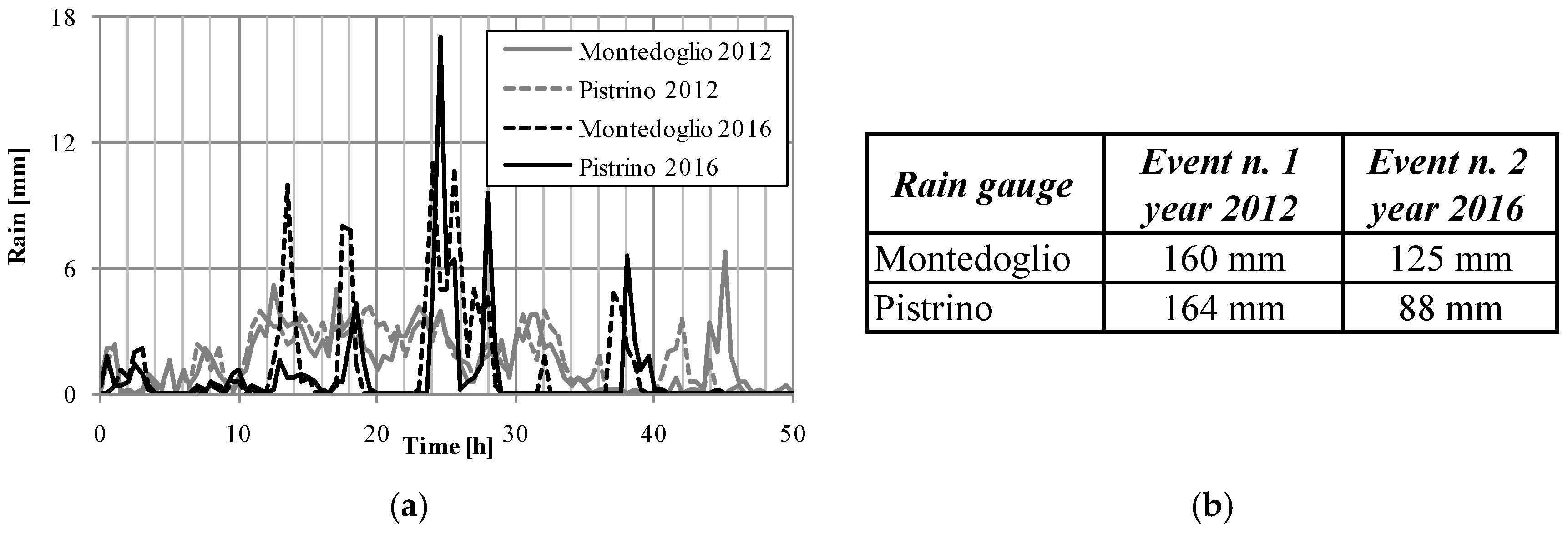
The proposed methodology is tested using historical data of two flood events; the first one occurred in the year 2012 and the second one in the year 2016. The rainfall series measured at each rain gauge, and shown in Figure 13 is applied to all the computational cells inside the watershed area and the corresponding polytope is defined by the Thiessen method [33].
The 2012 rainfall event is relatively continuous throughout the simulated 48 h and the maximum duration of a single storm is 29 h. During the 2016 event, the maximum duration of a single storm has been much shorter and equal to 6 h (Figure 13).
As a result of the short duration of the single storms and the large extension of the polytopes associated with each rain gauge, the mean rain depth over each polytope is likely to be smaller than the measured one. The Moisello and Papiri’s ARF method [30] is applied to take into account this reduction for the estimation of the rain P associated with each computational cell in the runoff model of Section 2.2.
As previously mentioned, a significant discharge enters into a culvert 520 m long in the flat urban area of Pistrino. When the discharge in the culvert exceeds 6 m3/s (as calculated by our next simulations), the flow overtops the inlet culvert, inundates the Pistrino urban area, and a large part of it leaves the basin through the left boundary of the catchment, along a very flat area, without passing through the outlet gauged section.
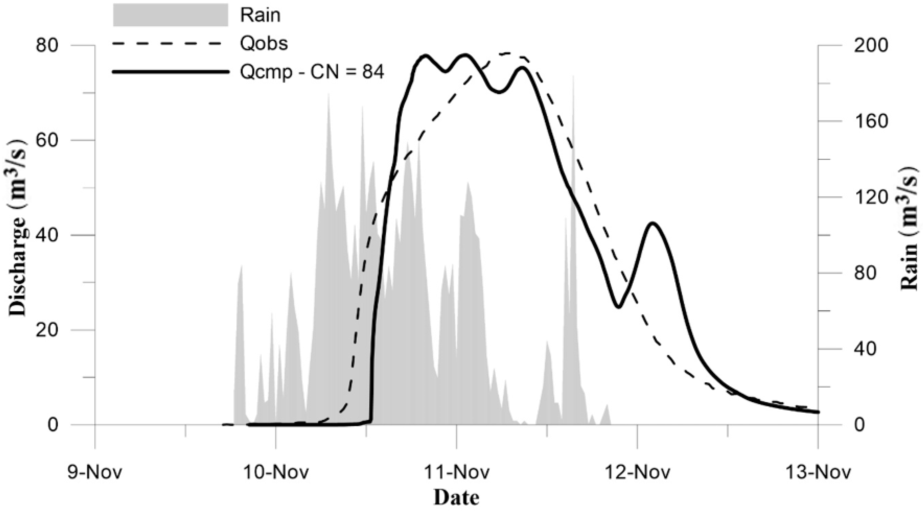
To compute the rainfall excess, CN and λ parameters are calibrated for the November 2012 event from the balance between the inlet and outlet volumes (8.913 Mm3), while the peak discharge is used to calibrate the Manning roughness n (Figure 14). For the hydraulic analysis, zero water depth is assigned as the initial condition. The calibrated parameters are CN = 84, λ = 0.01, and n = 0.050 s/m1/3. The observation that an initial abstraction ratio λ equal to 0.20, as suggested in [26], provides a strong delay of the simulated storm hydrograph with respect to the observed one, which is missing in the computed optimal one. The optimal CN parameter is also much higher than the regional values suggested in the literature [26]. This can be justified by the fully distributed structure of the proposed model, which simulates the water storage effect during the flow routing. The same effect is embedded in the CN parameters when the Curve Number method is applied for the discharge computation. In this first calibration event, the errors in the volume and peak discharge estimation are both close to 1.1%, and the Nash–Sutcliffe efficiency (NSE) is equal to 0.882.
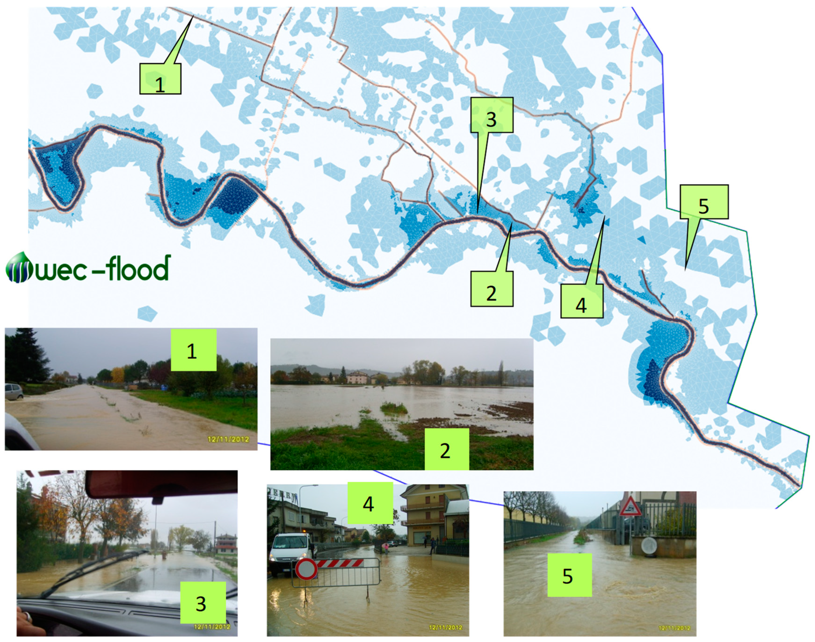
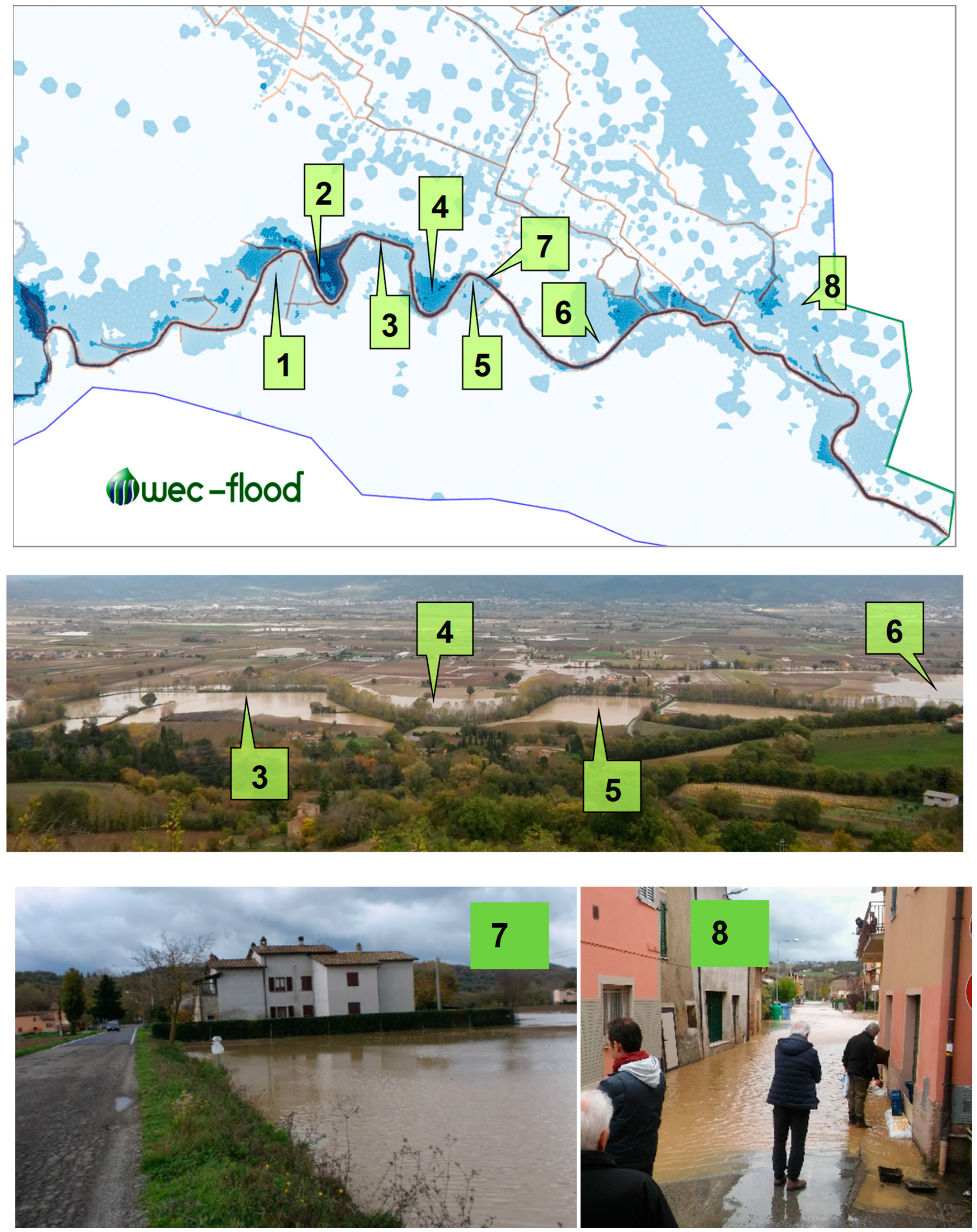
The historically flooded areas have been estimated from the images of the pictures taken immediately after the two events and show a good qualitative match with the results of the proposed method. The computed and the historical maximum flooded areas in the 2012 event are compared in Figure 15.
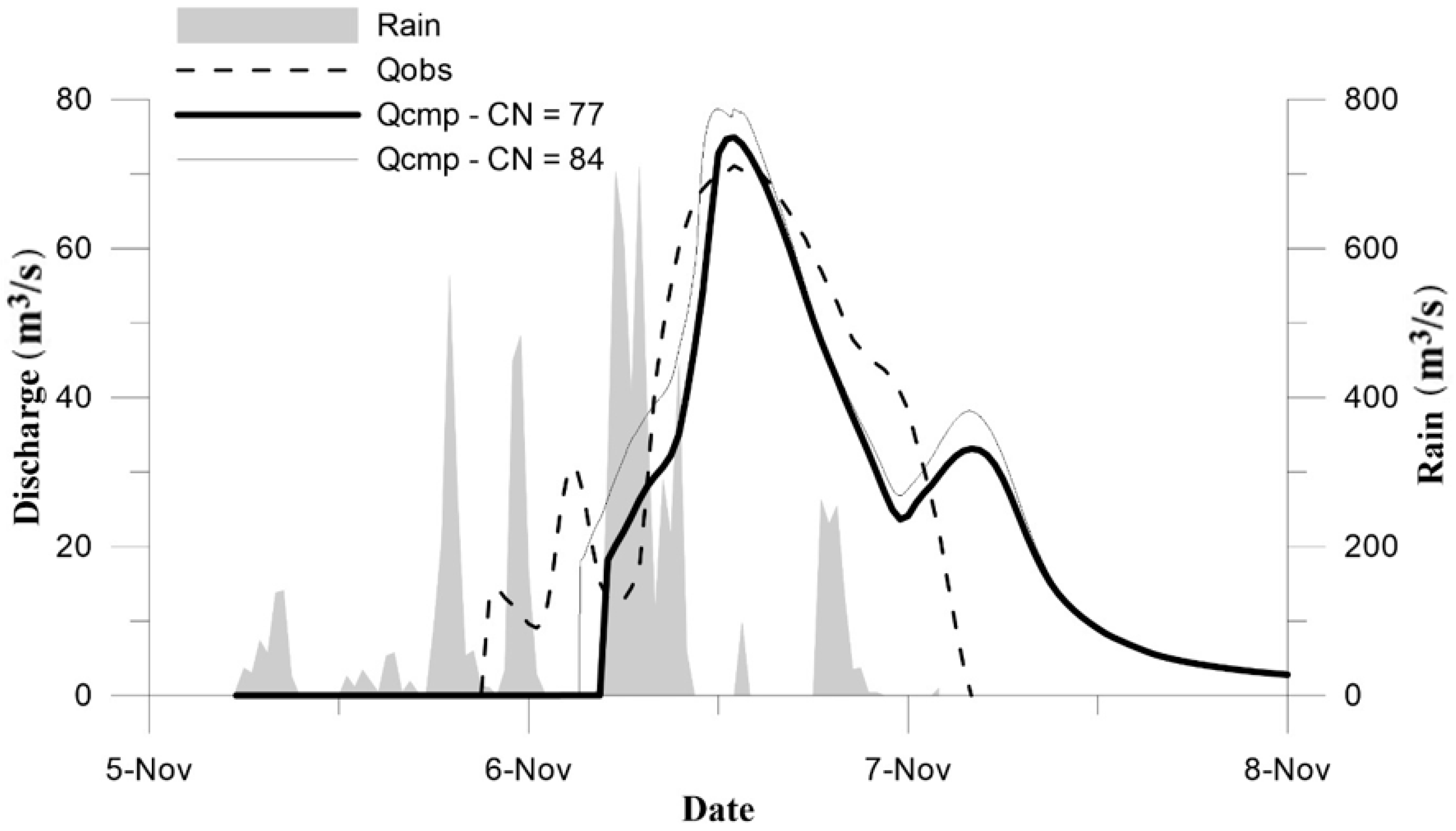
The same parameters n = 0.050 s/m1/3, CN = 84, and λ = 0.01, calibrated for the 2012 event, have been used to simulate the 2016 event. The observation that the CN parameter is a function of the ground saturation level and, is used in the context of nowcasting, should be corrected according to the actual saturation level. The errors between computed and observed hydrographs otherwise grow up to 14.5% and 10.2%, respectively, for the volume and for the peak discharge, but the shape of the computed hydrograph is quite similar to the measured one. The NSE found in this validation event is equal to 0.776. The relatively small impact of the CN parameter is confirmed by its optimization for the 2016 flood event. In this case, the optimal value of CN equal to 77 allows to drop the errors up to 0.3% and 4.7%, respectively for the volume and for the peak discharge but leads to anNSE equal to 0.753, similar to the previous one. The results obtained for the 2016 event are shown in Figure 16. In both events, the differences between the measured and the computed discharges are likely to depend mainly on the actual heterogeneity of the rainfall distribution, which has been accounted for in the model only through the ARF reduction of the mean value over each polytope.
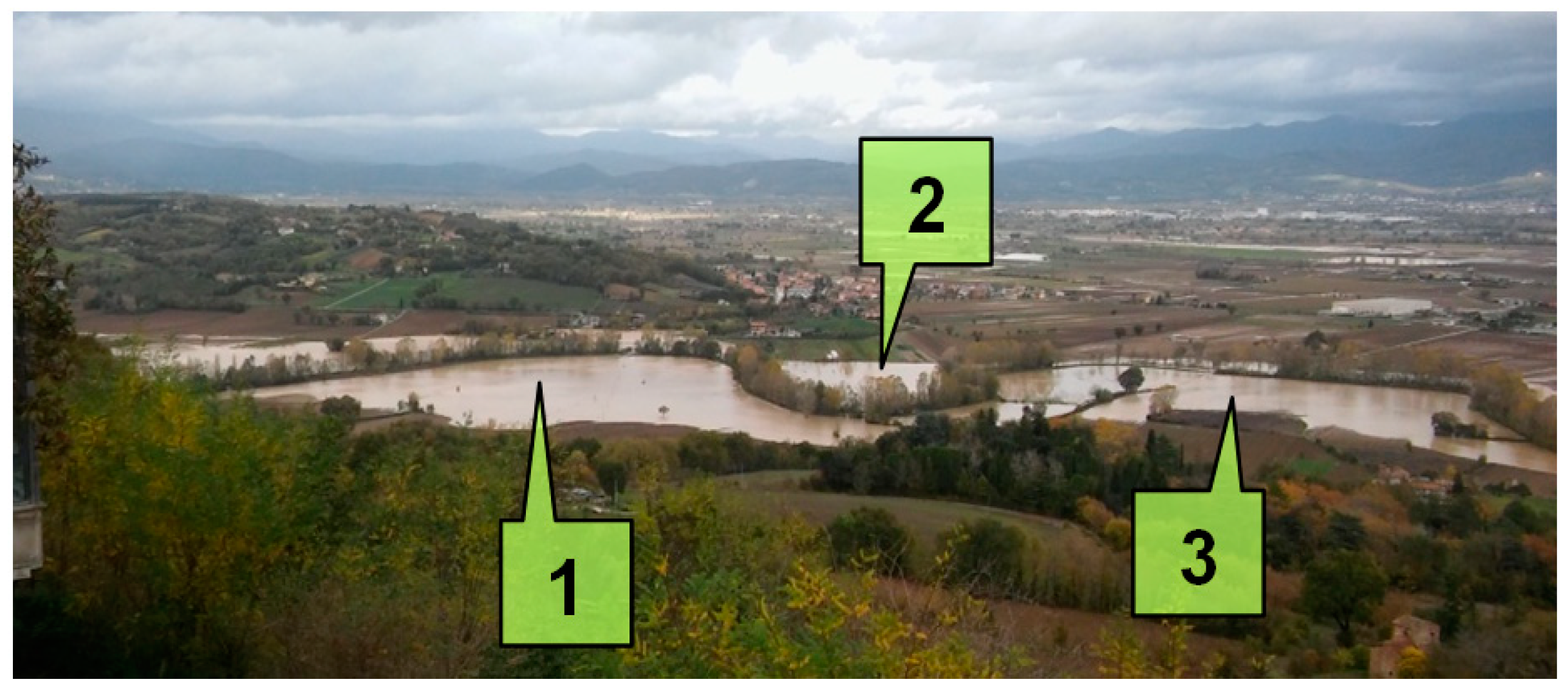
Some pictures of the flooded urban areas taken immediately after the 2016 event, have been used to estimate the maximum water depths, assuming the CN value is equal to 77, as shown in Figure 17. Specifically, picture 8 shows that the flood overtopped the culvert during the flood and the flood wave inundated the Pristino urban area.
5. Conclusions
An efficient engineering tool for a reliable delineation of flooded areas has been developed and applied to a test case in central Italy. The tool only requires, along with the hydraulic input (rain, initial, and boundary conditions), the DEM of the area and the vectors of other elevation points, representing anthropic elements, such as roads or urban river embankments. The major innovation of the procedure is its capability of generating a TIN and a set of nodal topographic elevations performing two different tasks—(1) to be a suitable computational mesh for both the hydrologic and the shallow water hydraulic models (with required regularity properties), (2) to form with some of its edges, a hydrographic network of previously assigned density. The density heterogeneity of the mesh allows good performance of the model in both the urban and the upstream areas inside the same computational domain.
In spite of the scarcity of data available for calibration, the resulting hydraulic model has provided, in the test case, good reconstruction of two historical events, with the use of only three parameters. In the first event, used for calibration, the resulting NSE was 0.882. In the second event, applied with the same calibrated parameters, the resulting NSE was 0.776. As in other cases, and well documented in literature, the major uncertainty of the results is likely due to the uncertainty in the temporal and spatial distribution of the rainfall, as well as in the knowledge of the domain topography and of the initial soil conditions. In spite of this, the availability of a single tool for the simulation of the entire chain of hydrologic transformation leading to the flood is of major interest, because it allows the construction of a direct relationship between the structural entities (like a culvert or a bank) and the resulting predicted water depths and velocities. In the context of the Building Image Modeling (BIM), this could easily become, in the near future, one of the several tools required by political decision-makers for good urban planning [34].
Finally, considering that this approach is self-contained in generating channel networks, very simple to simulate runoff formation and reliable in the diffusive-based flooding area assessment, it well lends itself to be applied at a larger scale, and this will be the next research challenge.
Author Contributions
Conceptualization, T.T., M.S. and C.N.; methodology, T.T., T.M., M.S. and C.N.; software, T.T. and M.S.; Investigation, C.N.; resources, S.B. and C.M.; writing—original draft preparation, M.S. and C.N.; writing—review and editing, T.T. and T.M. All authors have read and agreed to the published version of the manuscript.
Funding
This research received no external funding.
Conflicts of Interest
The authors declare no conflict of interest.
Appendix A. Mathematical Statement of the Constrained Minimization (CM) Problem and Computation of the “Upper” Auxiliary Solution
The DEM correction problem is cast as the solution of the following constrained minimization problem:
where is the measured elevation datum in cell i, zcmi is the corrected one, ic(i,m) is the index of the mth cell surrounding cell i in any of the eight available directions, ε is a minimum slope (parameter), ci,m is the distance between the center of the two cells, i and ic(i,m), Nc is the total number of cells, as well as the index of the outlet cell. The elevation of the basin outlet cell is not subject to then constraint (A2). We call the solution of problem (A1) and (A2) an optimal solution.
i = 1, …, Nc − 1
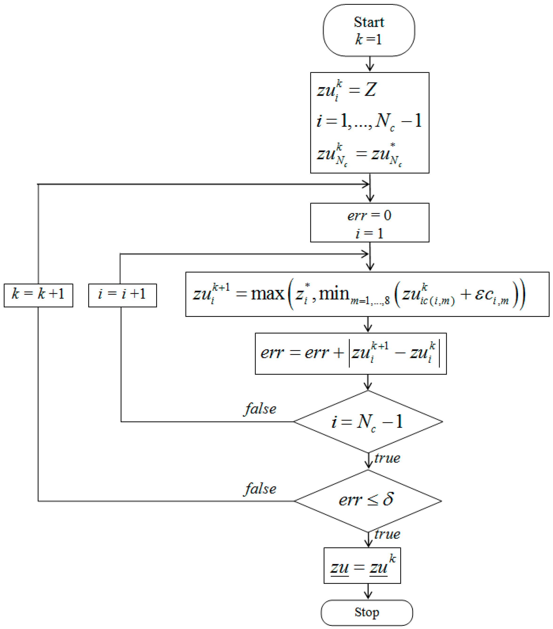
The “upper” solution zu is initialized by setting all the zui cell elevations equal to Z, except the basin outlet one. Z is the maximum cell elevation in the basin, and the elevation zuNc of the basin outlet cell always remains the measured one.
If k is the index of the iteration cycle, for each k value initializing with zero residue R, a loop m is computed on all the domain cells, except the outlet one. In each cell update, the “upper” solution elevation is calculated as follows:
where ε is a small arbitrary number, m is the index direction, ici,m is the index of the cell neighbor to cell i in the mth direction, ci,m is the distance between the centers of cells i and ici,m. The eight possible directions are Nord, Nord-Est, Est, Sud-Est, Sud, Sud-West, West, Nord-West (Figure A1). If the cell is a boundary cell, one or more directions will be missing. Updating the residue with:
After the end of the loop with index i, residue R is checked. If R is smaller than a small positive number δ, k is increased and the next iteration is started, otherwise stopped. See the flow-chart of the “upper” solution computation in Figure A2.
Figure A1.
Directions of cells next to cell i.

Figure A2.
Flow chart of the “upper” solution.

Appendix B. Computation of the “Lower” Auxiliary Solution
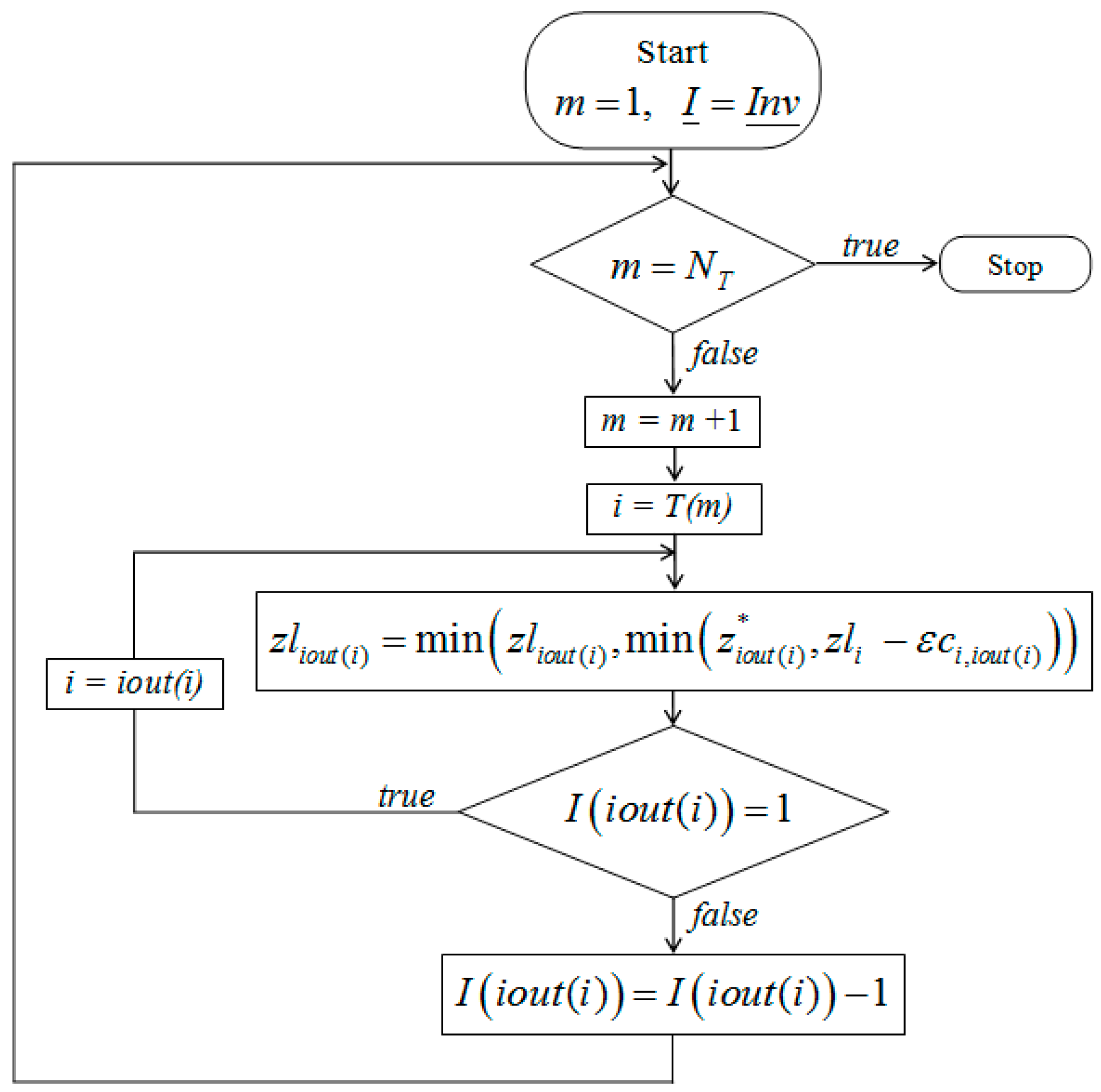
Say Inv(i) is the number of cells with any index m drained by cell i, such that for a number Inv(i) of cells with index m condition Iout(m) = i holds. Say leaf cell a cell i with Inv(i) = 0 and NT the number of the leaf cells. Say T(m) the cell index of the mth leaf cell. The “lower” solution zl is initialized by setting all the zl(i) cell elevations equal to Z, except the leaf cells, where we set zl(i) = z*(i). This also initializes an auxiliary vector I(i) = Inv(i).
Say k is the leaf index and starts from k = 1. Set i = T(k) and update zl(Iout(i)) with the following formula:
If iout(i) = Nc (the outlet cell index) and I(Nc) = 1 stop; If iout(i) ≠ Nc and I(Nc) = 1 set i= iout(i) and go back to operator (1B); If iout(i) ≠ Nc and I(Nc) > 1 set k = k + 1 and start again from i = T(k). See the flow chart of the “lower” solution computation in Figure A3.
Figure A3.
Flow chart of the “lower” solution.

Appendix C. Optimal Combination of the “Upper” and the “Lower” Solutions
Say Nb(j) the number of cells of the jth branch and Iz(i) the branch index associated to cell i. Assume Iz(i) = 0 if zui = zli. Call Ar(j) the cell index of the root of the jth branch, such that Iz(Iout(Ar(j))) = 0. Say A(j,k) the cell index of the kth element of the jth branch. Search for the optimal combination of the “upper” and “lower” solutions in each branch, given by:
To do that, minimize in each branch j the square error given by:
that is equivalent to set:
Appendix D. Correction of the TIN Node Elevations
To avoid the existence of artificial local minima, due to the interpolation error, an “upper” solution of the ground elevation of the TIN node elevation is found, following the same strategy used for the correction of the cell center elevations (see Appendix A). Equation (A3) changes into:
where id(i,m) is the index of the mth connected node, nste(i) is the number of nodes connected to node i and Nn is the total number of nodes, including the node at the center of the DEM outlet cell, which is assumed to have index Nn.
Appendix E. Culvert Modelling
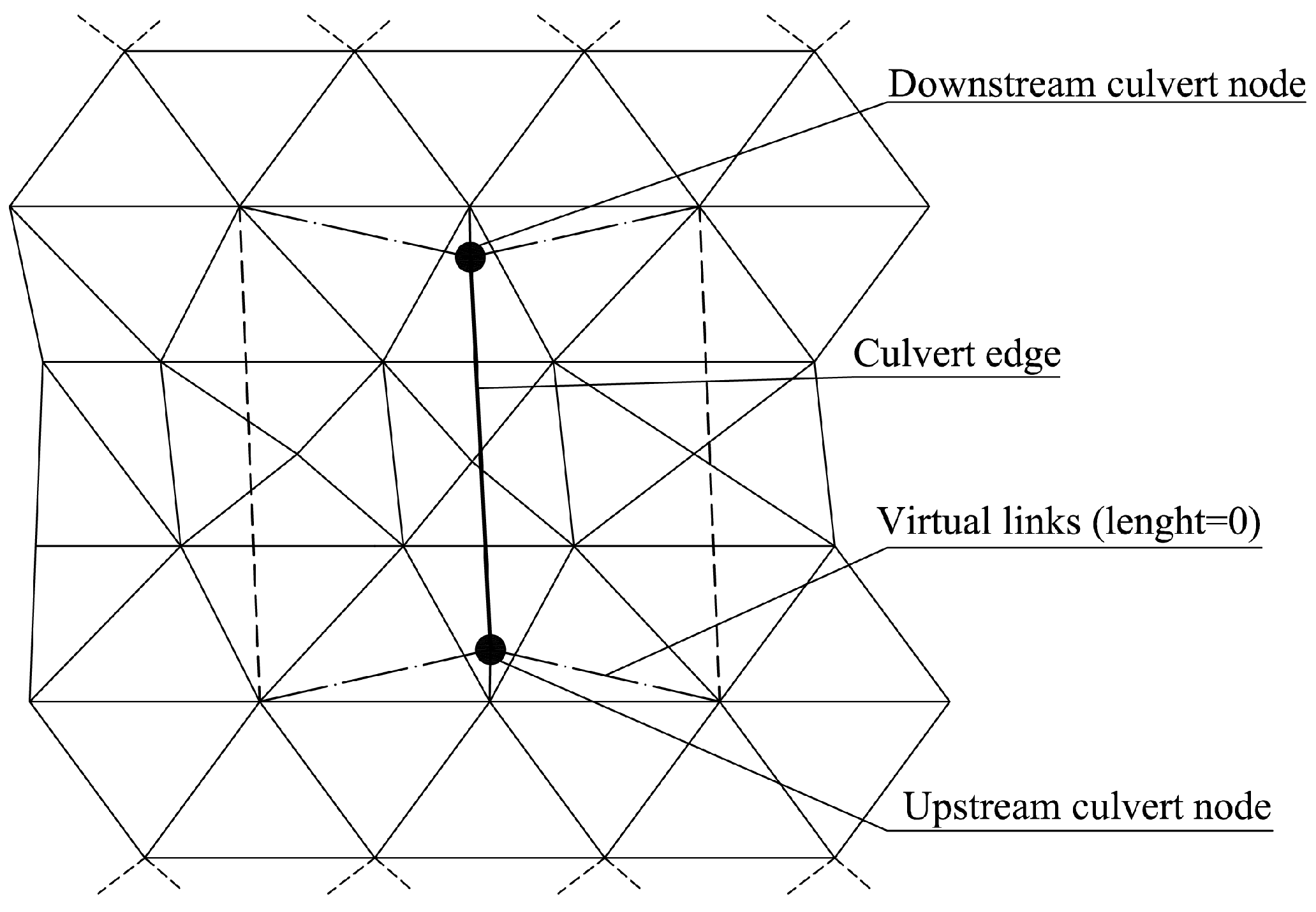
The hydraulic model used in the proposed methodology assumes that one or more nodes of the 2D domain overlap the inlet section of the culvert and that the cells of these nodes are connected with 1D channel cells by mixed edges, linking a computational cell of the 2D domain with a computational cell of the culvert 1D domain. Mixed edges can be thought of as simple topological entities, with zero length and storage capacity, having the only purpose of transferring the discharge from the 2D nodes to the culvert nodes and vice versa. Figure A4 shows an example of a 2D domain with three nodes aligned along the inlet and the outlet sections of a culvert. Three mixed edges link the three nodes with the first (and the last) section of a culvert, that has the real width bounded by the dotted lines.
Figure A4.
Schematic view of the proposed computational scheme.

In the prediction sub-problem, the fluxes are computed along the time step integration k + 1, in each edge m of the 1D sub-domain, as:
where is the conveyance associated to the culvert section, h is the water depth and is the piezometric gradient computed at the end of the kth time step. Mixed edges take the piezometric gradient of the channel edge connected to their culvert section and conveyance, which is a fraction c of the conveyance of the same channel edge. Because the conveyance per unit width is well-known to be almost proportional to the power 5/3 of the water depth, the fraction cs,i of the mixed edge linking culvert section s with the ith 2D node is computed at the end of the previous time step as:
where is the water depth in the 2D node n squared to 5/3, and the sum is extended to all the mixed edges connected to the culvert section s.
When the input discharge of the computational cell of a standard culvert section, shared by two or more channel edges, overcomes the maximum discharge allowed by the piezometric gradient, the water depth attains the maximum level in the culvert section and the exceeding discharge is restored in the sections during the solution of the next corrective sub-problem. When the same occurs in the 2D node connected to a culvert section through a mixed edge, the exceeding discharge is partially stored on the ground and partially transferred to the computational cell of another 2D node with lower potential, located also in the 2D domain above the culvert (see Figure A4).
References
- Sheth, M. Review: Rainfall Runoff Modelling. Int. J. Eng. Res. Technol. 2018, 7, 235–237. [Google Scholar]
- Beven, K.J. Rainfall-Runoff Modelling: The Primer; John Wiley & Sons: New York, NY, USA, 2000. [Google Scholar]
- Brath, A. Modelli matematici di formazione dei deflussi di piena. In La Sistemazione dei Corsi D’Acqua Naturali; Maione, U., Brath, A., Eds.; Editoriale Bios: Cosenza, Italy, 1996. [Google Scholar]
- Rodriguez-Iturbe, I.; Valdes, J.B. The Geomorphologic Structure of Hydrologic Response. Water Resour. Res. 1979, 15, 1409–1420. [Google Scholar] [CrossRef] [Green Version]
- Noto, L.V.; La Loggia, G. Derivation of a distributed unit hydrograph integrating Gis and remote sensing. J. Hydrol. Eng. 2007, 12, 639–650. [Google Scholar] [CrossRef]
- Mishra, A.; Hata, T. A grid-based runoff generation and flow routing model for the Upper Blue Nile basin. Hydrol. Sci. 2006, 51, 191–206. [Google Scholar] [CrossRef]
- Looper, J.P.; Vieux, B.E. An assessment of distributed flash flood forecasting accuracy using radar and rain gauge input for a physics-based distributed hydrologic model. J. Hydrol. 2012, 412–413, 114–132. [Google Scholar] [CrossRef]
- Kim, J.; Warnock, A.; Ivanov, V.Y.; Katopodes, N.D. Coupled modeling of hydrologic and hydrodynamic processes including overland and channel flow. Adv. Water Resour. 2012, 37, 104–126. [Google Scholar] [CrossRef]
- Teng, J.; Jakeman, A.J.; Vaze, J.; Croke, B.F.W.; Dutta, D.; Kim, S. Flood inundation modelling: A review of methods, recent advances and uncertainty analysis. Environ. Model. Softw. 2017, 90, 201–216. [Google Scholar] [CrossRef]
- Chena, A.S.; Evans, B.; Djordjević, S.; Savić, D.A. A coarse-grid approach to representing building blockage effects in 2D urban flood modelling. J. Hydrol. 2012, 426–427, 1–16. [Google Scholar] [CrossRef] [Green Version]
- Shi, Z.-H.; Chen, L.-D.; Fang, N.-F.; Qin, D.-F.; Cai, C.-F. Research on the SCS-CN initial abstraction ratio using rainfall-runoff event analysis in the Three Gorges Area, China. Catena 2009, 77, 1–7. [Google Scholar] [CrossRef]
- Planchon, O.; Darboux, F. A fast, simple and versatile algorithm to fill the depressions of digital elevation models. Catena 2001, 46, 159–176. [Google Scholar] [CrossRef]
- Aricò, C.; Sinagra, M.; Begnudelli, L.; Tucciarelli, T. MAST-2D diffusive model for flood prediction on domains with triangular Delaunay unstructured meshes. Adv. Water Resour. 2001, 34, 1427–1449. [Google Scholar] [CrossRef] [Green Version]
- Aricò, C.; Filianoti, P.; Sinagra, M.; Tucciarelli, T. The FLO diffusive 1D-2D model for simulation of river flooding. Water 2016, 8, 200. [Google Scholar] [CrossRef] [Green Version]
- Popescu, I.; Jonoski, A.; Van Andel, S.J.; Onyari, E.; Moya Quiroga, V.G. Integrated modelling for flood risk mitigation in Romania: Case study of the Timis–Bega river basin. Int. J. River Basin Manag. 2010, 8, 269–280. [Google Scholar] [CrossRef]
- Wang, Y.; Chen, A.S.; Fu, G.; Djordjević, S.; Zhang, C.; Savić, D.A. An integrated framework for high-resolution urban flood modelling considering multiple information sources and urban features. Environ. Model. Softw. 2018, 107, 85–95. [Google Scholar] [CrossRef]
- Tanaka, T.; Yoshioka, H.; Siev, S.; Fujii, H.; Fujihara, Y.; Hoshikawa, K.; Ly, S.; Yoshimura, C. An Integrated Hydrological-Hydraulic Model for Simulating Surface Water Flows of a Shallow Lake Surrounded by Large Floodplains. Water 2018, 10, 1213. [Google Scholar] [CrossRef] [Green Version]
- Grimaldi, S.; Schumann, G.J.-P.; Shokri, A.; Walker, J.P.; Pauwels, V.R.N. Challenges, opportunities and pitfalls for global coupled hydrologic-hydraulic modeling of floods. Water Resour. Res. 2019, 55, 5277–5300. [Google Scholar] [CrossRef] [Green Version]
- Nogherotto, R.; Fantini, A.; Raffaele, F.; Di Sante, F.; Dottori, F.; Coppola, E.; Giorgi, F. An integrated hydrological and hydraulic modelling approach for the flood risk assessment over Po river basin. Nat. Hazards Earth Syst. Sci. Discuss. 2019. [Google Scholar] [CrossRef]
- Aureli, F.; Prost, F.; Vacondio, R.; Dazzi, S.; Ferrari, A. A GPU-Accelerated Shallow-Water Scheme for Surface Runoff Simulations. Water 2020, 12, 637. [Google Scholar] [CrossRef] [Green Version]
- Jenson, S.K.; Domingue, J.O. Extracting topographic structure from digital elevation data for geographic information systems. Photogram. Eng. Rem. Sens. 1988, 54, 1593–1600. [Google Scholar]
- Martz, L.W.; Garbrecht, J. An outlet breaching algorithm for the treatment of closed depressions in a raster DEM. Comput. Geosci. 1999, 25, 835–844. [Google Scholar] [CrossRef]
- Soille, P. Optimal removal of spurious pits in grid digital elevation models. Water Resour. Res. 2004, 40, W12509. [Google Scholar] [CrossRef] [Green Version]
- Grimaldi, S.; Nardi, F.; Di Benedetto, F.; Istanbulluoglu, E.; Bras, R.L. A physically-based method for removing pits in digital elevation models. Adv. Water Resour. 2007, 30, 2151–2158. [Google Scholar] [CrossRef]
- Zhu, D.; Ren, Q.; Xuan, Y.; Chen, Y.; Cluckie, I.D. An effective depression filling algorithm for DEM-based 2-D surface flow modelling. Hydrol. Earth Syst. Sci. 2013, 17, 495–505. [Google Scholar] [CrossRef] [Green Version]
- U.S. Department of Agriculture. Estimation of Direct Runoff from Storm Rainfall. In National Engineering Handbook Part 630 Hydrology; National Resources Conservation Service: Washington, DC, USA, 2004. [Google Scholar]
- Xu, Y.; Fu, B.; He, C.; Gao, G. Watershed discretization based on multiple factors and its application in the Chinese Loess Plateau. Hydrol. Earth Syst. Sci. Discuss. 2011, 8, 9063–9087. [Google Scholar] [CrossRef]
- Huang, M.; Gallichand, J.; Wang, Z.; Goulet, M. A modification to the Soil Conservation Service curve number method for steep slopes in the Loess Plateau of China. Hydrol. Process. 2006, 20, 579–589. [Google Scholar] [CrossRef]
- Lim, K.J.; Engel, B.A.; Muthukrishnan, S.; Harbor, J. Effects of initial abstraction and urbanization on estimated runoff using CN technology. J. Am. Water Resour. Assoc. 2007, 42, 629–643. [Google Scholar] [CrossRef]
- Moisello, U.; Papiri, S. Relation between areal and point rainfall depth. In Proceedings of the XX Congress “Idraulica e Costruzioni Idrauliche”, Padua, Italy, 8–10 September 1986. (In Italian). [Google Scholar]
- Spada, E.; Sinagra, M.; Tucciarelli, T.; Barbetta, S.; Moramarco, T.; Corato, G. Assessment of river flow with significant lateral inflow through reverse routing modeling. Hydrol. Process. 2017, 31, 1539–1557. [Google Scholar] [CrossRef]
- Aricò, C.; Tucciarelli, T. A Marching in space and time (MAST) solver of the shallow water equations. Part I: The 1D case. Adv. Wat. Res. 2007, 30, 1236–1252. [Google Scholar] [CrossRef]
- Chow, V.T.; Maidment, D.R.; Mays, L.W. Applied Hydrology; McGraw-Hill Book Company: NewYork, NY, USA, 1988. [Google Scholar]
- Azhar, S. Building information modeling (BIM): Trends, benefits, risks, and challenges for the AEC industry. Leadersh. Manag. Eng. 2011, 11, 241–252. [Google Scholar] [CrossRef]
Figure 1.
Flowchart of the proposed Hydronet algorithm.

Figure 2.
The eight neighboring cells surrounding a generic cell i inside the basin and the corresponding directions. The possible location of the cell iout(i) is also shown.
Figure 2.
The eight neighboring cells surrounding a generic cell i inside the basin and the corresponding directions. The possible location of the cell iout(i) is also shown.

Figure 3.
(a) zp bilinear interpolation area. (b) zp linear variation along the fixed edge.

Figure 4.
Computational mesh.

Figure 5.
Schematic view of river flooding due to culvert overtopping.

Figure 6.
Sovara stream basin in central Italy.

Figure 7.
Digital Elevation Model adopted for the case study (resolution 10 m × 10 m).

Figure 8.
Sovara stream basin—hydrographic network computed with different values of the Sill threshold ratio.
Figure 8.
Sovara stream basin—hydrographic network computed with different values of the Sill threshold ratio.

Figure 9.
Comparison of the Digital Elevation Model correction between the Hydronet and the “filling up” method.
Figure 9.
Comparison of the Digital Elevation Model correction between the Hydronet and the “filling up” method.

Figure 10.
Detail of the mesh along the Sovara stream close to the urban area of Pistrino.

Figure 11.
Sovara stream basin: final computational mesh.

Figure 12.
Location of the culvert and of the rain meters in the computational domain.

Figure 13.
(a) Hyetographs and (b) total rainfall depths observed during the two investigated flood events.
Figure 13.
(a) Hyetographs and (b) total rainfall depths observed during the two investigated flood events.

Figure 14.
November 2012 flood event: comparison between observed rainfall, observed and computed discharge hydrographs at the hydrometric section of Pistrino (basin outlet).
Figure 14.
November 2012 flood event: comparison between observed rainfall, observed and computed discharge hydrographs at the hydrometric section of Pistrino (basin outlet).

Figure 15.
Computed flooded areas and some pictures that were taken during the 2012 event.

Figure 16.
The November 2016 flood event: a comparison between the observed rainfall, and the observed and computed discharge hydrographs at the hydrometric section of Pistrino (basin outlet).
Figure 16.
The November 2016 flood event: a comparison between the observed rainfall, and the observed and computed discharge hydrographs at the hydrometric section of Pistrino (basin outlet).

Figure 17.
Computed flooded areas and some pictures taken during the 2016 event.


Table 1.
Sequence of computed elevation vectors.
| Vector Name | Description |
|---|---|
| zcm | Optimal solution of the Constrained Minimum (CM) problem, never found |
| zu | “Upper” auxiliary solution of the CM problem |
| zl | “Lower” auxiliary solution of the CM problem |
| zc | Sub-optimal solution of the CM problem, linear combination of zu and zl |
| zp | TIN node elevations, interpolated from zc elevation in the cell centers and from other point elevations |
| z | Corrected final elevation in the TIN nodes |
© 2020 by the authors. Licensee MDPI, Basel, Switzerland. This article is an open access article distributed under the terms and conditions of the Creative Commons Attribution (CC BY) license (http://creativecommons.org/licenses/by/4.0/).
Share and Cite
MDPI and ACS Style
Sinagra, M.; Nasello, C.; Tucciarelli, T.; Barbetta, S.; Massari, C.; Moramarco, T. A Self-Contained and Automated Method for Flood Hazard Maps Prediction in Urban Areas. Water 2020, 12, 1266. https://doi.org/10.3390/w12051266
AMA Style
Sinagra M, Nasello C, Tucciarelli T, Barbetta S, Massari C, Moramarco T. A Self-Contained and Automated Method for Flood Hazard Maps Prediction in Urban Areas. Water. 2020; 12(5):1266. https://doi.org/10.3390/w12051266
Chicago/Turabian StyleSinagra, Marco, Carmelo Nasello, Tullio Tucciarelli, Silvia Barbetta, Christian Massari, and Tommaso Moramarco. 2020. "A Self-Contained and Automated Method for Flood Hazard Maps Prediction in Urban Areas" Water 12, no. 5: 1266. https://doi.org/10.3390/w12051266
Note that from the first issue of 2016, this journal uses article numbers instead of page numbers. See further details here.