In-Situ Monitoring and Characteristic Analysis of Freezing-Thawing Cycles in a Deep Vadose Zone
by
 , , , ,
Ce Zheng
1,2 ,
,
Yudong Lu
1,
Xiuhua Liu
1,3,*,
Jiří Šimůnek
2 ,
,
Yijian Zeng
4,
Changchun Shi
5 and
Huanhuan Li
1 1
Key Laboratory of Subsurface Hydrology and Ecological Effects in Arid Region of Ministry of Education, School of Water and Environment, Chang’an University, Xi’an 710054, China
2
Department of Environmental Sciences, University of California, Riverside, CA 92521, USA
3
Shaanxi Key Laboratory of Land Consolidation, Chang’an University, Xi’an 710064, China
4
Faculty of Geo-Information and Earth Observation (ITC), University of Twente, Hengelosestraat 99, 7514 AE Enschede, The Netherlands
5
China State Long-Term Observation and Research Station for Mu Us Desert Ecosystem in Yulin of Shaanxi, Yulin 719000, China
*
Author to whom correspondence should be addressed.
Water 2020, 12(5), 1261; https://doi.org/10.3390/w12051261
Submission received: 20 February 2020
/
Revised: 25 April 2020
/
Accepted: 27 April 2020
/
Published: 29 April 2020
(This article belongs to the Section Hydrology)
Abstract
:Freeze-thaw cycles play a critical role in affecting ecosystem services in arid regions. Monitoring studies of soil temperature and moisture during a freeze-thaw process can generate data for research on the coupled movement of water, vapor, and heat during the freezing-thawing period which can, in turn, provide theoretical guidance for rational irrigation practices and ecological protection. In this study, the soil temperature and moisture changes in the deep vadose zone were observed by in-situ monitoring from November 2017 to March 2018 in the Mu Us Desert. The results showed that changes in soil temperatures and temperature gradients were largest in soil layers above the 100-cm depth, and variations decreased with soil depth. The relationship between soil temperature and unfrozen water content can be depicted well by both theoretical and empirical models. Due to gradients of the matric potential and temperature, soil water flowed from deeper soil layers towards the frozen soil, increasing the total water content at the freezing front. The vapor flux, which was affected mainly by temperature, showed diurnal variations in the shallow 20-cm soil layer, and its rate and variations decreased gradually with increasing soil depths. The freeze-thaw process can be divided into three stages: the initial freezing stage, the downward freezing stage, and the thawing stage. The upward vapor flux contributed to the formation of the frozen layer during the freezing process.
1. Introduction
Regions with frozen soil are widely distributed in middle and high latitudes, affecting approximately 50% of the land around the world [1,2]. Soils in these regions will freeze or thaw in response to variations in soil temperatures, resulting in the phase change of soil water among ice, liquid water, and water vapor [3,4,5]. Abundant forest and mineral resources exist in these areas, and the frozen soil, representing a vital factor of the biological environment, affects productive activities and the sustainable development of these resources [6]. As the research of the critical zone increases in scope, studies on the dynamics in soil temperature and moisture in the vadose zone during freezing-thawing periods have attracted a growing interest [7,8].
The freeze-thaw process has a substantial impact on the surface energy balance and soil moisture distribution, significantly affecting soil properties, such as soil structure, permeability, conductivity, and bulk density, making it difficult and complicated to study water flow, heat transport, and related parameters in seasonally frozen soils [9,10,11]. For instance, the freezing process reduces soil and air permeabilities, influences the heat exchange, and changes the distribution of soil water. Furthermore, phase transitions of soil water occur frequently due to freeze-thaw cycles, resulting in variations in unfrozen water contents at subzero temperatures [12,13]. Physical properties of frozen soil in cold regions are strongly dependent on temperature when unfrozen water is present, and both unfrozen water and soil temperature control the freeze-thaw process and soil water migration [2,14,15]. Also, the presence of salts can alter the freeze-thaw process in soils and their transport during the freeze-thaw period could lead to increased soil salinization [16,17]. The coexistence of unfrozen water and ice in frozen soil affects its hydrological and thermal properties, becoming a significant factor for many engineering and environmental applications [18]. During the freezing process, unfrozen water flows in the direction of soil matric potential and temperature gradients from unfrozen soil in deeper soil layers, increasing the water content of the frozen layer [19,20,21]. The total soil water during the freezing period can be divided into “freezable” unfrozen water, absorbed water, and unfreezable water [22,23].
In arid areas with a deep groundwater level, moisture migration in the vadose zone often takes place in the form of water vapor [24,25], and the transformation between liquid water and water vapor occurs continuously, which results in water vapor playing a key role in maintaining surface vegetation and ecosystems [26,27]. Water vapor, driven mainly by temperature gradients, flows from warmer to cooler soil layers and performs a critical function in affecting variations in soil water contents in the vadose zone [28,29]. The existing literature indicates that vapor flow has a significant influence on variations in soil water contents during the freeze-thaw process under such conditions [24,30]. Both liquid water and water vapor flow upward towards the freezing front, and it is water vapor that connects water transfer below the freezing front and above the evaporation front [30]. Furthermore, since water vapor fluxes can become larger than liquid water fluxes in deep soil layers, only a model considering the coupled movement of water, vapor, and heat can fully describe critical physical mechanisms of the hydrological cycle in the vadose zone [31].
Many studies have evaluated coupled interactions between water and heat, and the influence of freeze-thaw cycles on soil properties. However, most of these studies were carried out either in laboratories or in areas with shallow groundwater, which have obvious spatial limitations [14,32]. Therefore, in-situ monitoring of the deep vadose zone is highly needed to improve our understanding of dynamic changes in the spatial-temporal distributions of moisture and temperature in frozen soils. Moreover, monitoring studies of soil water and heat movement under the freeze-thaw process in a deep vadose zone can provide data required for the development and validation of models simulating the coupled movement of water, vapor, and heat under such conditions, as well as for establishing practical guidance for rational irrigation management and ecological protection.
Therefore, the objectives of this study were (i) to monitor the soil temperature and moisture changes of the 8-m deep vadose zone in the Mu Us Desert during freezing-thawing periods, (ii) to analyze spatial and temporal distributions of soil temperatures and water contents, and (iii) to evaluate water vapor fluxes in the soil profile using Fick’s law.
2. Materials and Methods
2.1. Study Site
The Mu Us Desert is located between the Ordos Plateau and the Loess Plateau in northwestern China (Figure 1), in the north part of the Shaanxi Province, northeast of the Ningxia Hui Autonomous Region, and south of the Inner Mongolia Autonomous Region. The climate in the desert can be characterized as dry and cold, with large temperature differences and frequent strong winds. Based on the meteorological data since 1961, annual temperatures range from −31.4 to 36.4 °C, with an average annual temperature of 6.4 °C. Mean annual precipitation and potential evaporation are 360 and 2343 mm, respectively, and over 60% of the annual rainfall occurs from July to September [33,34]. Total annual sunshine time exceeds 3000 h, with total radiation of 608.37 kJ/cm2. The Mu Us Desert is typically subject to seasonal freezing, with the freeze-thaw process from November to March. The frozen layer usually extends to 100 cm below the soil surface.
The Mu Us Desert is one of the most vulnerable ecological areas in China. With rapid economic development and large-scale construction of energy bases, groundwater resources have been extensively developed, resulting in a significant decline in the groundwater level and an increase in the vadose zone thickness [35,36,37]. During the freezing period, diurnal temperature changes have a considerable effect on soil water movement, and dynamics in soil water contents and temperatures are closely related to vegetation growth, land desertification, and geologic hazards.
2.2. In-Situ Observations
The field work was conducted at the Yu Lin Desert Ecosystem Research Station (longitude 109°42′29″ E, latitude 38°23′19″ N, at an altitude of 1157 m above the sea level). At the study site, sand is the dominant soil fraction in the active soil layer and the land cover is dominated by Salix Pasmmophila and Artemisia. Vegetation is sparse during the freezing period, covering less than 5% of the land surface. As shown in Figure 1, a monitoring well with a diameter of 150 cm was dug to a depth of 900 cm, which is below the groundwater table (the groundwater level was located at a soil depth of 852 cm on 1 November 2017). Soil samples were collected to conduct the particle size analysis (Table 1). Sand and clay accounted for approximately 95% and 1% of the soil mass in the vadose zone, respectively, except for the soil horizon between 80 and 230 cm, where the clay content was slightly higher. For the measurements not to be influenced by external meteorological conditions, the well was covered by a 15 cm thick piece of polyethylene foam with the thermal conductivity of 0.03 W/m/K and a 10 cm thick well cover.
Monitoring sensors were installed at different depths of the soil profile through the wall of the well (Table 2). To minimize the influence of the well itself on measured values, the average distance of sensors from the wellbore was 50 cm. Monitoring started 6 months after the sensors were installed to allow soil to settle and establish better contact with the sensors. The Hydra Probe II sensors, which are based on the frequency domain (FD) measurement principles, were calibrated using gravimetric measurements (samples were oven-dried at 105 °C for 24 h; gravimetric water contents were converted to volumetric water contents using the soil bulk density) on soil samples collected from the study site. The concept of unfrozen water content measurements is based on the confirmed similarity between soil drying-wetting and freezing-thawing processes [3,38]. When testing at 100 MHz, the permittivity of liquid water (≈78) is significantly higher than those of the soil matrix (≈3–5), ice (≈3.4) and air (≈1) [15,38,39]. Moreover, the soil permittivity of the liquid phase is much more sensitive to soil temperature changes than those of solids and air [40]. Therefore, observed soil water contents were assumed to represent unfrozen water contents when the soil was frozen. Soil samples collected from different depths during the freezing period were taken to the laboratory to determine the total water content by an oven drying method. All sensors in the monitoring well were linked to a solar-powered automatic data-logger (CR1000), which recorded data at a 10 min interval. An automatic micrometeorological station was installed to record related meteorological variables at a 30 min interval, such as wind speed, air temperature, relative humidity, and precipitation. The observed data at the study site, from 1 November 2017 to 31 March 2018, was collected to analyze the variations in soil temperature and moisture during the freeze-thaw process.
Figure 2 shows the mean, maximum, and minimum air temperatures during the observation period. Air temperatures varied greatly during each day, with a mean diurnal temperature range of 22.8 °C, which dropped sharply in November and then increased in March. The mean temperature of the coldest month (January) and warmest month (March) during the study period reached −11.5 and 6.1 °C, respectively. Rainfall and snow during the study period were only 20.8 mm. It is clear that snow had little effect on variations in the unfrozen water content at shallow depths during the freezing period (Figure 2b,c).
2.3. Mathematical Calculations
2.3.1. Soil Heat Transport
Many analytical solutions of the soil energy balance equation coupled with Fourier’s law exist. One of them holds for homogeneous soils, no flow conditions, and an upper boundary condition given by a temperature sine wave with average temperature T0 (°C), a temperature amplitude A0 (°C), the time period τ (e.g., 24 h or 365 day), and a constant (both temporally and spatially) thermal diffusivity KT [41]:
where T is the temperature (°C), t is time (h), z is depth (cm), d is the damping depth (cm), ω is the angular frequency (h−1), and φ is the phase constant (-). The damping depth d and the diurnal amplitude Az (°C) at depth z can be calculated as follows:
2.3.2. Unfrozen Water Content
Based on the analogy between freezing and drying processes and the assumption that the ice pressure is equal to zero at freezing conditions, the relationship between soil subfreezing temperature and the liquid water matric potential can be expressed using the generalized Clapeyron equation [13]:
where h is the liquid water matric potential (m), Lf is the latent heat of vaporization (approximately 3.34 × 10⁵ J/kg), g is the gravitational acceleration (=9.81 m/s2), T is the temperature (K), and T0 is the freezing point of liquid water (=273.15 K).
According to the van Genuchten [42] model, the soil–water characteristic curve, which relates the water content with the pressure head, is as follows:
where θl, θr, and θs are the liquid, residual, and saturated water contents (m3/m3), respectively, and α (m−1), n (-), and m (-) are empirical parameters. The soil hydraulic parameters can be estimated from soil physical properties using neural network-based pedotransfer functions implemented in the numerical model HYDRUS-1D [43]. Equations (4) and (5) can be used to characterize the soil freezing characteristics curve to predict the unfrozen soil water content with measured subfreezing temperatures instead of measured pressure heads.
Additionally, an empirical method proposed by Xu et al. [44] can estimate the variations of unfrozen water contents with subfreezing temperatures:
where coefficients a and b are empirical constants that depend on soil texture and the initial water content. These two coefficients can be estimated using two (subscripts 1 and 2) freezing temperatures Tf (°C) and corresponding unfrozen water content θ (m3/m3) data pairs as follows:
2.3.3. Thermal Vapor Flux
In general, the vapor density ρv (kg/m3), which is used to calculate water vapor fluxes, can be calculated as a function of the saturated vapor density ρsv (kg/m3) and relative humidity Hr as follows [45]:
The saturated vapor density can be expressed as a function of temperature:
and the relative humidity Hr can be calculated using a thermodynamic relationship between liquid water and vapor in the soil as follows:
where M is the molecular weight of water (=0.018015 kg/mol) and R is the universal gas constant of water vapor (=8.315 J/mol/K).
The thermal vapor flux qv (m/s) can be calculated using Fick’s Law:
where KvT is the thermal vapor hydraulic conductivity (m2/K/s), which can be expressed as follows:
where D is the vapor diffusivity in soil (m2/s), which is defined as D = Daθaτ, where Da is the vapor diffusivity in air (=2.12 × 10⁻⁵(T/273.15)2 m2/s), θa is the air-filled porosity (m3/m3), τ is the tortuosity factor (=θa7/3/θs2) [46], ρw is the density of liquid water (kg/m3), and η is the enhancement factor (-) that can be calculated as follows [47]:
where fc is the mass fraction of clay in the soil (-).
3. Results
3.1. Measured Spatial-Temporal Distribution of Soil Temperature
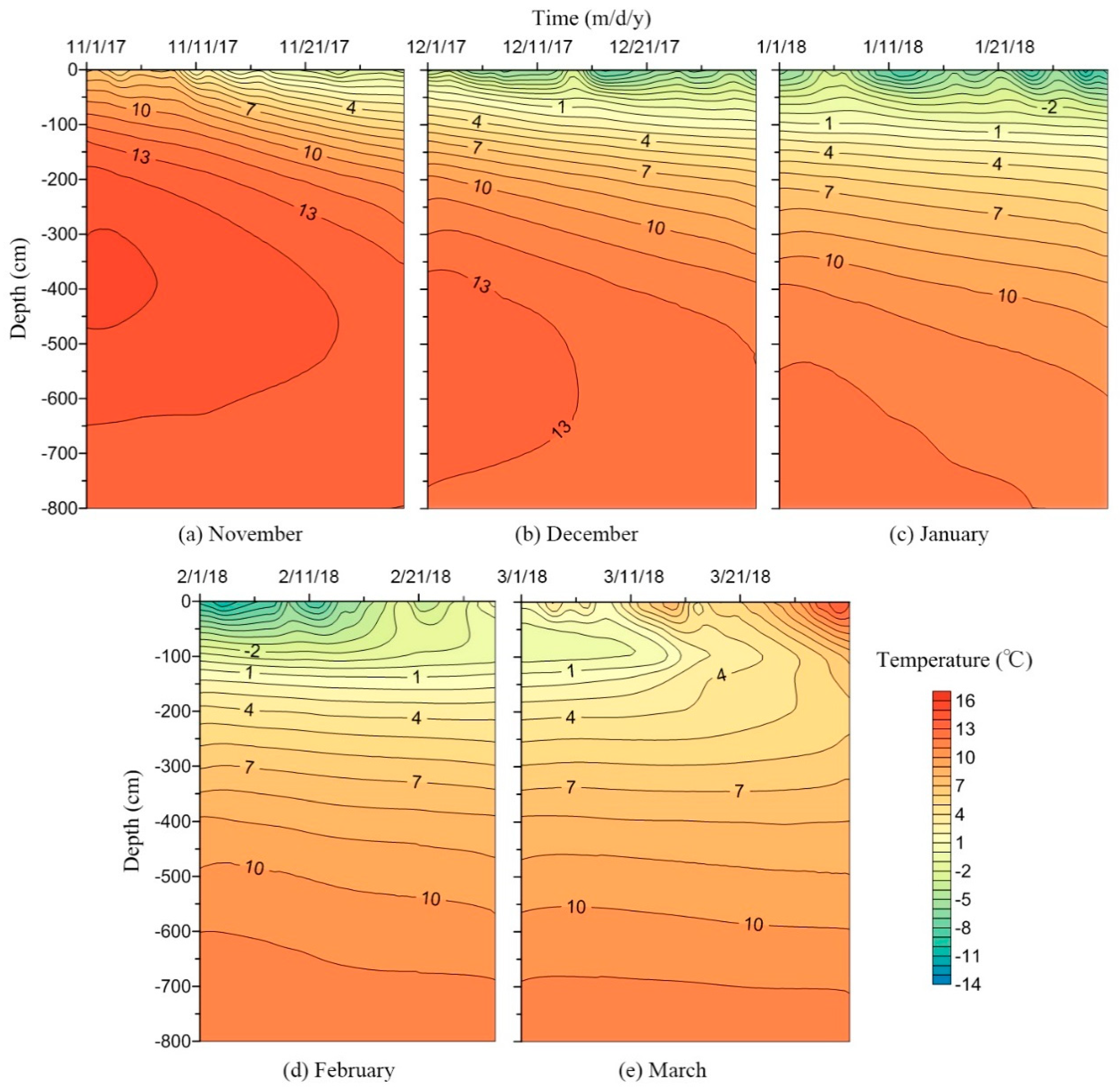
The spatial-temporal distribution of soil temperature measured during the observation period is shown in Figure 3. At the beginning of monitoring, soil temperatures in the upper part of the vadose zone were relatively low, while the maximum temperature (15.4 °C) was observed at a depth of 400 cm, resulting in an upward temperature gradient. As air temperatures kept falling after November, soil temperatures decreased accordingly and were invariably higher than air temperatures, resulting in the soil being exothermic. Due to a persistent upward heat flux, the depth of the maximum soil temperature in the vadose zone continued to increase, eventually reaching the 800 cm depth on 1 January. During this time period, the heat flux recorded by HFP01 at a depth of 800 cm decreased from a positive (downward) value of 0.76 W/m2 to a negative (upward) value of −0.02 W/m2, which was consistent with observed soil temperatures. Measured data indicated that soil temperatures above a depth of 200 cm reached their lowest values gradually in February and subsequently rose with an increase in air temperatures, especially in the top 50 cm layer, where they exceeded 10 °C. As a result, soil temperatures between depths of 100 and 200 cm became the lowest throughout the vadose zone. It should be noted that soil temperatures in the lower part of the vadose zone retained a slowly decreasing trend, even at the end of the observation period.
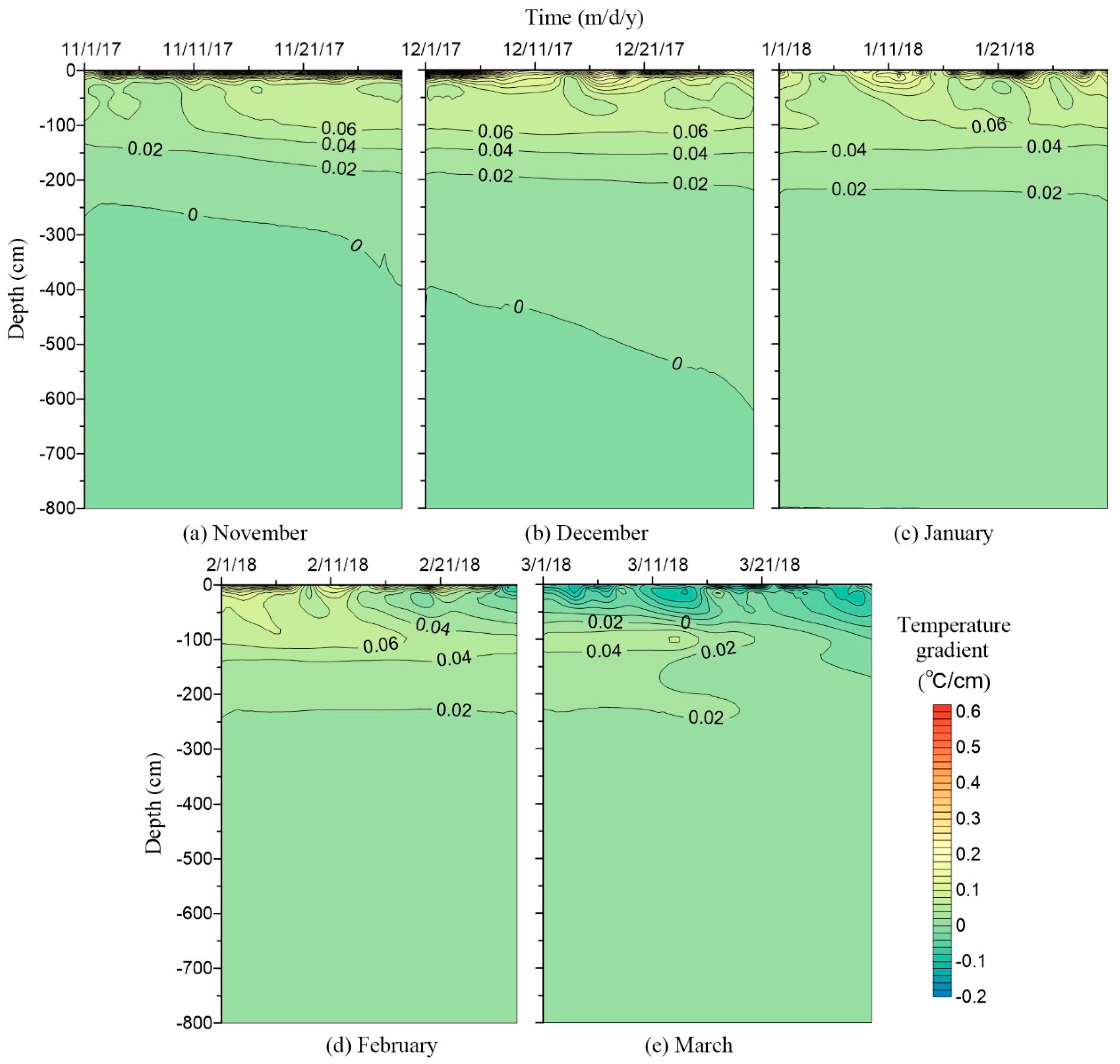
It is evident that the spatial distribution of temperature gradients (Figure 4) is consistent with soil temperatures, with temperature gradients decreasing with increasing soil depths. Note that variations in temperature gradient at soil depths above the 20 cm depth differed greatly (about 1–2 orders of magnitude) from those at deeper soil layers. During the freezing period, the temperature gradient varied from 0.248 to 0.055 °C/cm between the soil surface and a depth of 100 cm, reflecting obvious variations in soil temperature in this layer. On the contrary, temperature gradients were relatively low in the lower parts of the vadose zone. During the thawing period, the soil layer above a depth of 100 cm displayed negative (downward) temperature gradients, especially in the top 20 cm depths, with the gradients ranging from −0.102 to −0.051 °C/cm.
Table 3 provides a list of quantitative variables characterizing variations of soil temperatures at different depths. During the observation period, soil temperatures at depths of 2, 10, and 20 cm ranged from −12.4 to 15.9 °C, −10.1 to 14.0 °C, and −8.6 to 13.1 °C, respectively, and were significantly affected by changes in air temperatures (with correlation coefficients of 0.952, 0.938, and 0.899, respectively). The range of temperature variations decreased with depth, and the temperature changes became relatively small below the 200 cm depth (less than 10 °C). Furthermore, the coefficient of variation (Cv), as expected, decreased as the soil depth increased, indicating a weakening trend in soil temperature variations with depth.
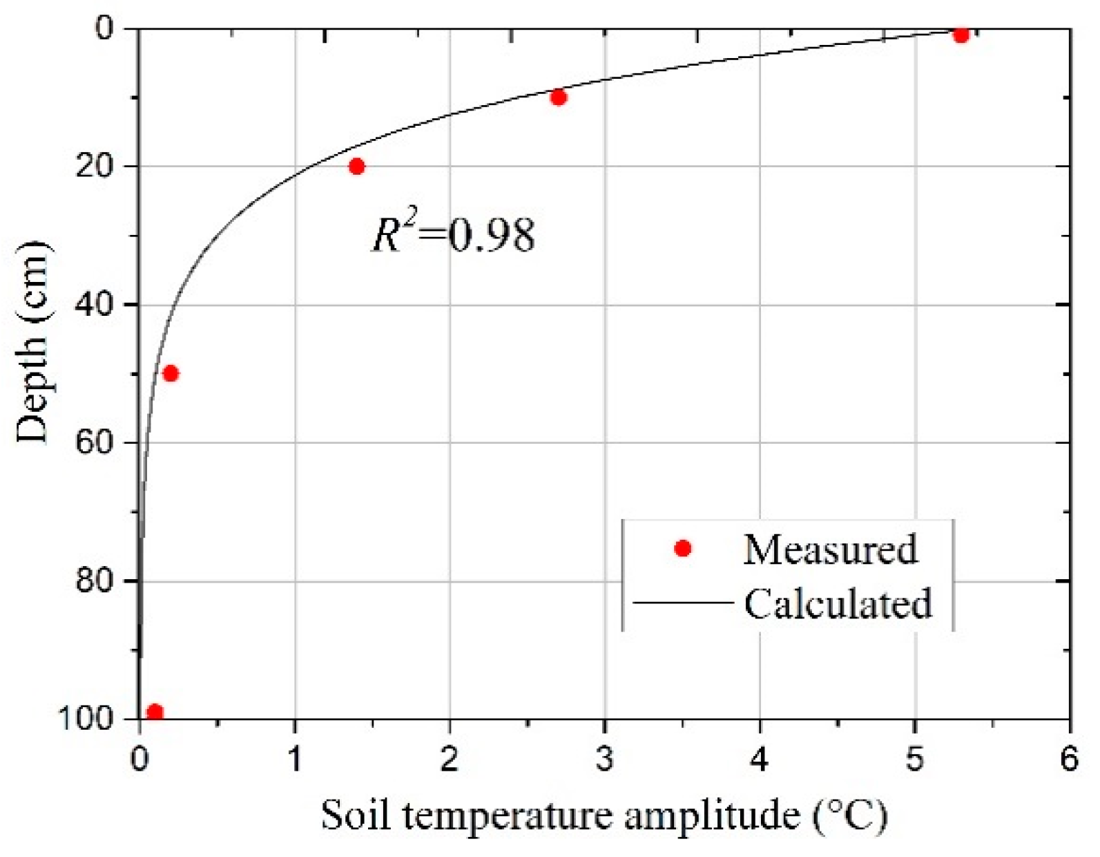
As the soil in this study is relatively dry (as discussed below in detail), the effect of the specific heat of freezing/thawing can be neglected, and the Equation (3) can be used to approximate soil temperatures with depth at subzero temperatures as well. Figure 5 illustrates measured and calculated (with T0 = −2.1 °C, A0 =5.4 °C, and KT =20.7 cm2/h) diurnal soil temperature amplitudes as a function of depth. The results show that calculated and measured temperature amplitudes agreed well, with a correlation coefficient of 0.98. The observed diurnal temperature amplitude at the soil surface, and at depths of 10 and 20 cm, were 5.4, 2.7, and 1.4 °C, respectively, while the amplitude became much smaller (less than 0.1 °C) below the 100 cm depth. Calculated values were always slightly lower than measured values, which was mainly because the measured amplitude at a depth of 2 cm was adopted to represent temperature variations at the soil surface, resulting in a lower value of the diurnal temperature amplitude at the surface (A0).
3.2. Measured Spatial-Temporal Distribution of Soil Water Content
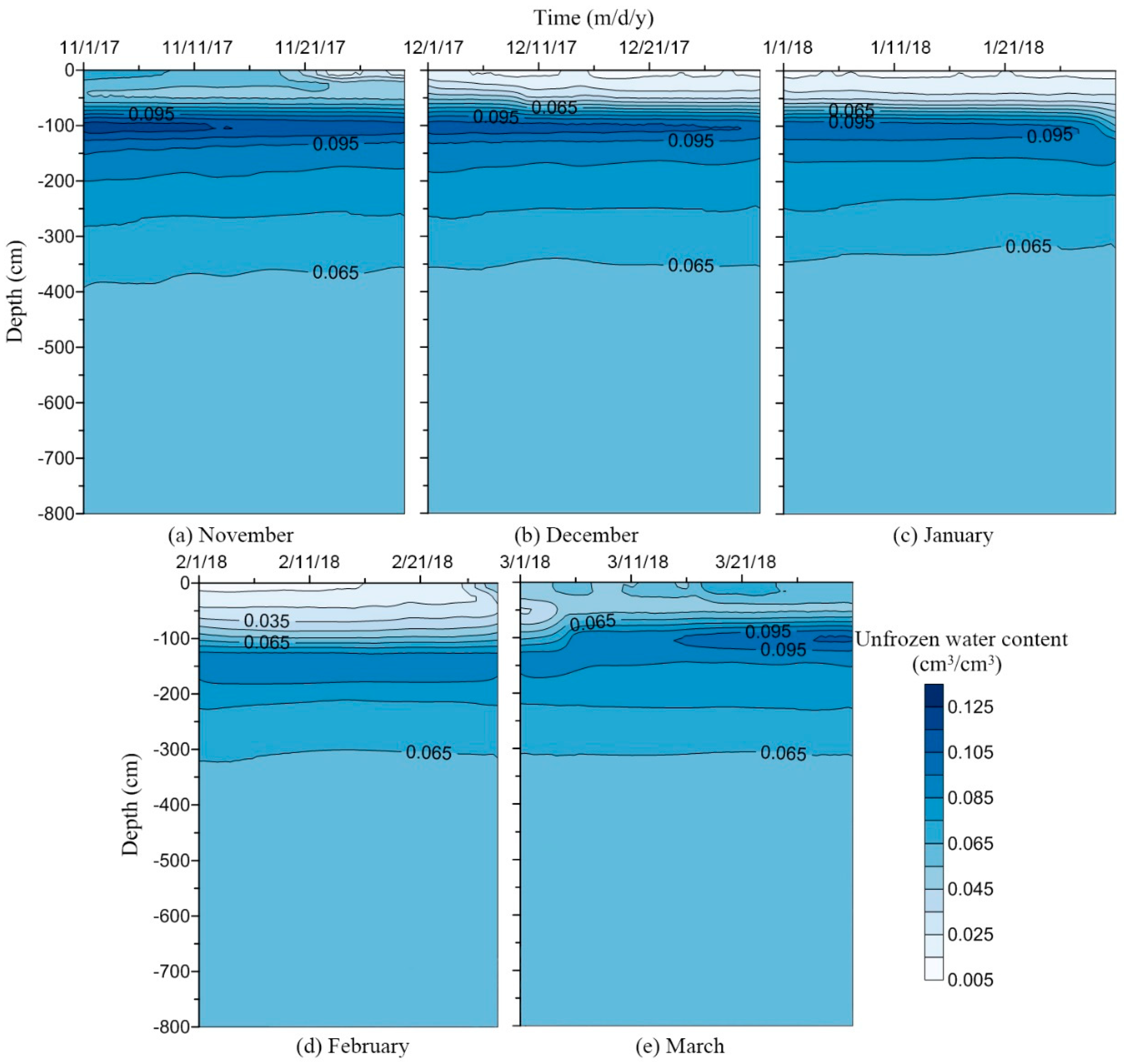
Figure 6 shows the spatial-temporal variations of the unfrozen water content during the observation period. The changes in the unfrozen water content were distinctive between the soil surface and a depth of 100 cm. Due to intensive solar radiation and sparse rainfall, the average water content in the soil profile was very low: approximately 0.06 cm3/cm3. During the freezing period, the unfrozen water content gradually decreased with time elapsed. The measured data showed a significant decrease in the unfrozen water content at depths of 10, 20, 50, and 100 cm on 24 November, 1 December, 10 December, and 26 January, respectively, demonstrating the phase change of liquid water. On the other hand, a decrease in the unfrozen water content below the 100 cm depth was only about, or less than, 0.01 cm3/cm3. As temperatures increased, the frozen layer gradually thawed after late February. Compared with the period before freezing, the soil water content changed after the frozen layer completely melted. For example, a decrease in the soil water content at a depth of 100 cm was about 16%, from 0.114 to 0.096 cm3/cm3. Since water contents were not affected by external factors, such as rainfall, this observation proves that the freeze-thaw process contributed to the redistribution of soil moisture in the soil profile. Meanwhile, the correlation coefficients between soil temperatures and unfrozen water contents were generally high with an average value of about 0.9 (as shown in Table 4), indicating similar trends (first decreasing and then increasing) in soil temperatures and water contents at corresponding depths. The minimum value (0.754) occurred at the 100 cm depth, which was mainly due to a sudden decrease in the unfrozen water content (Figure 6c) while soil temperature dropped gradually (Figure 3c).
A wetter soil layer with the soil water content from 0.08 to 0.12 cm3/cm3 existed between depths of 80 and 230 cm, which may be attributed to two factors. First, due to the temperature gradient, both liquid water and water vapor would flow upward and accumulate in this layer. Second, although the entire profile was mainly composed of sandy soil, the clay and silt fraction represented a considerable proportion (approximately 10%) of this soil layer, resulting in higher water retention and more restricted soil water movement in this layer.
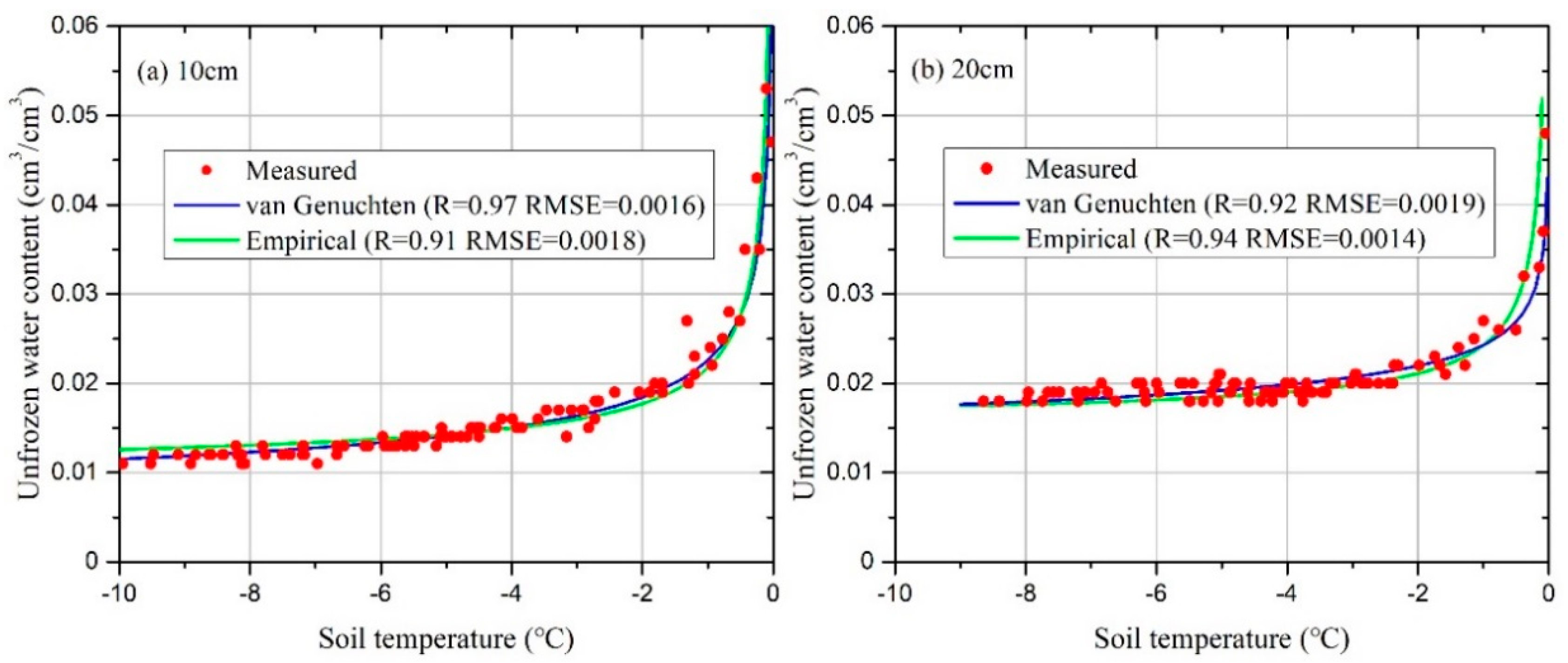
Figure 7 shows the relationship between the unfrozen water content and subfreezing temperature, and Table 5 lists the fitted parameters for both theoretical (Equation (5)) and empirical (Equation (6)) models. It is apparent that both models fitted observed data well at two different depths. The unfrozen water content began decreasing when soil temperature dropped below 0 °C, and the temperature range between 0 and −2 °C can be regarded as an apparent phase transformation temperature interval for the Mu Us sandy soil. In this temperature interval, a decrease in the unfrozen water content accounted for over 75% of the total water content. Most free water in the soil matrix froze in this temperature interval, and unfrozen water remained only in very small pores where ice cannot be easily formed. The downward trend in the unfrozen water content slowed when temperature ranged between −2 and −4 °C when unfrozen water consisted mainly of film water and absorbed water. Owing to this restriction, remaining unfrozen water (close to the residual water content) cannot easily freeze, and the change in the unfrozen water content became relatively low when soil temperature was below −4 °C. Also, the slope of the declining trend at a depth of 10 cm depth was steeper than at a depth of 20 cm. The minimum unfrozen water content was lower at a depth of 10 cm, which was mainly due to slightly different soil textures.
Table 6 lists the measured total water content and liquid water content data during the freezing period. The results indicated that the total soil water content above the depth of 50 cm displayed an increasing trend, especially in the shallow depth of 20 cm, and the ratio of liquid water content to the total water content gradually decreased with time elapsed. This phenomenon occurred mainly because a decrease in the unfrozen water content at the freezing front resulted in a sharp decline in the soil water potential, causing the unfrozen water from deeper soil layers to flow upward, towards the freezing front, and then to freeze there. Similarly, water vapor was flowing from deeper soil layers upward due to the temperature gradient (as discussed below in detail).
3.3. Water Vapor Flux
The calculation by Equation (9) showed that the vapor density remained in near-saturated conditions in the vadose zone during the non-freezing period, with the relative humidity reaching or acceding 99%. When the soil was frozen, the relative humidity declined with a decrease in the soil pressure head and temperature (e.g., it was about 90% at −10 °C), causing a reduction in the vapor density. Moreover, the results indicate that variations in soil temperature had a great influence on the vapor density. For example, a temperature increase of 1 °C would produce an increase of over 6% in the vapor density.
Figure 8 shows the distribution of the vapor density in the soil profile at three typical dates: before freezing (on 16 November), during the stable freezing stage (on 1 February), and after melting (on 25 March). Before the freezing period started, the vapor density was much smaller in the shallow soil layer than below it, while the maximum value of 12.5 × 10⁻⁶ g/cm3 occurred at the 400 cm depth. During the freezing period, the pressure head and soil temperatures in the frozen layer decreased sharply, resulting in a low vapor density and an upward vapor density gradient in the vadose zone. By comparison, the vapor density in the shallow layer increased significantly after melting, and the soil depth between 100 and 200 cm had the lowest vapor density (around 6.7 × 10⁻⁶ g/cm3). Additionally, the vapor density in the top 20 cm soil layer showed diurnal variations in all three cases, with an upward gradient of the vapor density during nighttime and a downward gradient of the vapor density during the daytime.
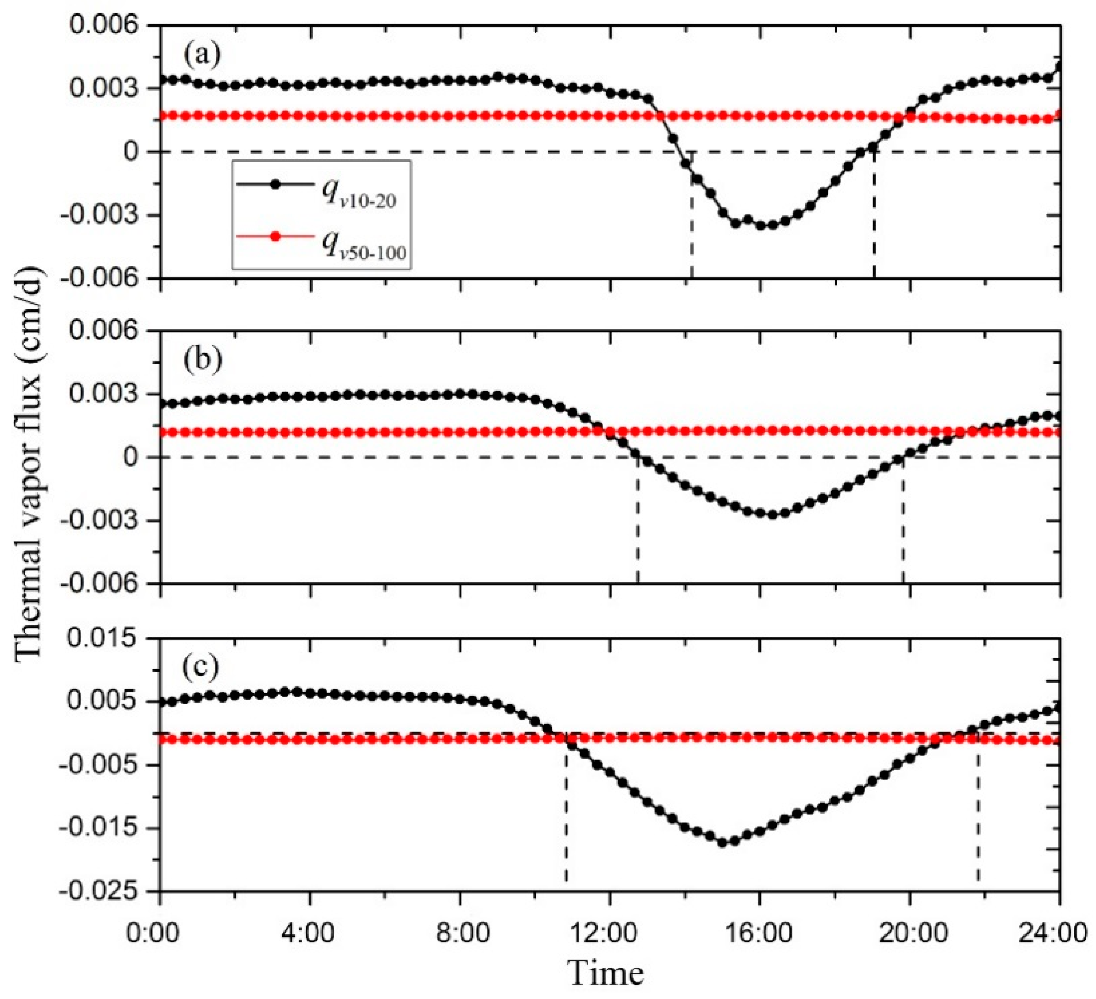
Figure 9 shows thermal vapor fluxes in the 10–20 and 50–100 cm soil layers on three typical days calculated using Equation (12). It is apparent that the vapor flux is affected by temperature changes in the shallow 20 cm depth. In this soil layer, on 16 November, water vapor flowed upward (about 0.003 cm/day at a depth of 10 cm) during most of the day, which was similar to variations on 1 February. However, with an increase in air temperature during the daytime, soil temperatures at the 10 cm depth were higher than at the 20 cm depth from 2:00 p.m. to 7:00 p.m. on 16 November and from 1:00 p.m. to 8:00 p.m. on 1 February, respectively, resulting in downward vapor flow during this time interval. Due to a rapid increase in air temperature after melting, the downward vapor flux sustained from 11:00 a.m. to 10:00 p.m. on 25 March. The maximum downward vapor flux was −0.017 cm/day, which was almost five times higher than before. For depths between 50 and 100 cm, soil temperatures fluctuated only slightly during the day, resulting in small vapor fluxes. While vapor fluxes were upward on 16 November (about 0.002 cm/day) and 1 February (about 0.001 cm/day), they were downward on 25 March (about −0.001 cm/day).
As for the deep soil layer, the vapor flux showed a decreasing trend with increasing soil depths. For example, owing to the relatively low temperature gradients, the thermal vapor fluxes at the 800 cm depth were −1.4 × 10⁻⁴, 1.6 × 10⁻⁴, and 2.9 × 10⁻⁴ cm/day on 16 November, 1 February, and 25 March, respectively.
4. Discussion
4.1. Characteristics of the Freeze-Thaw Process
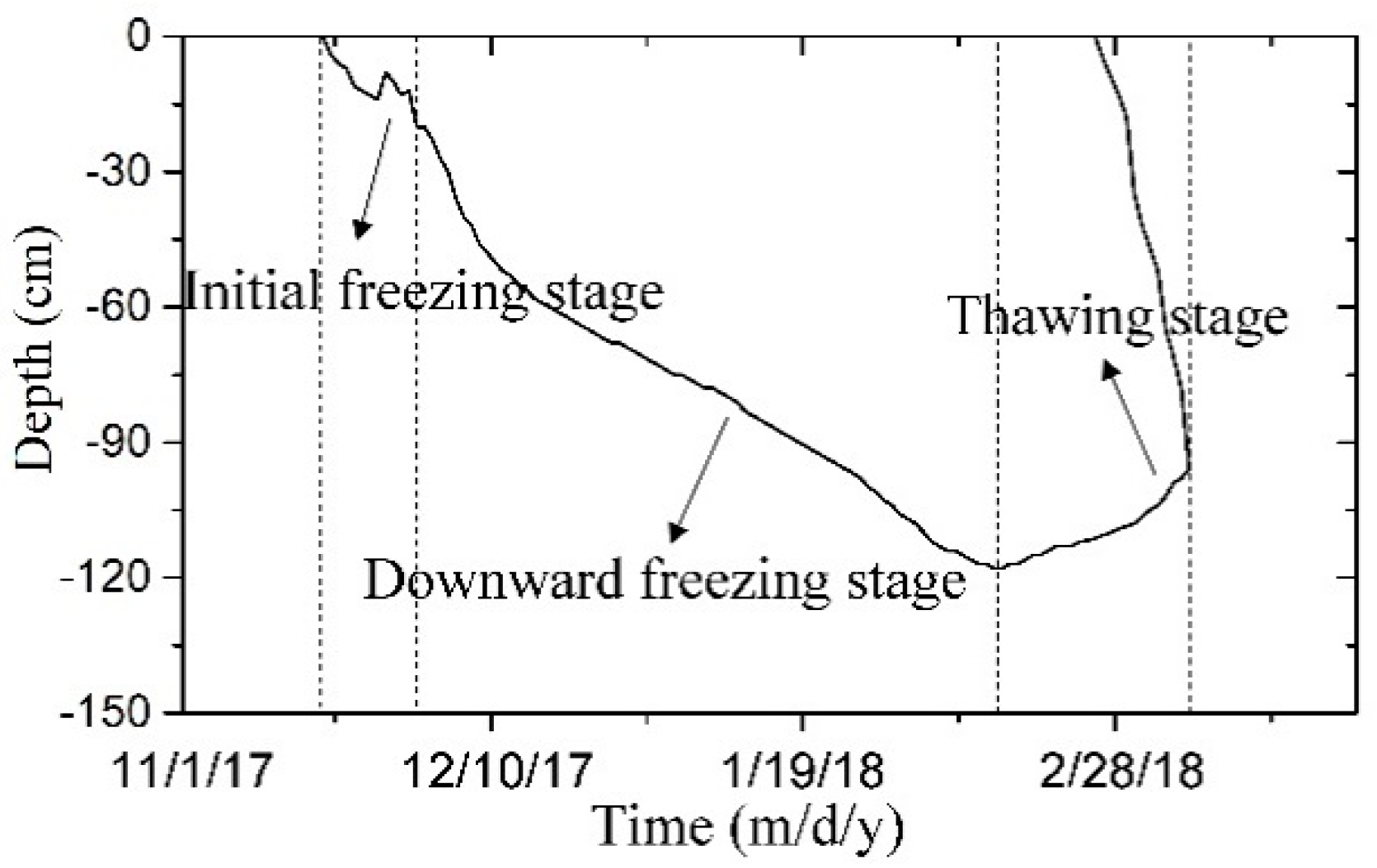
The freezing depth, defined as the depth with zero temperature, is often used to characterize the freeze-thaw process [9,26], as shown in Figure 10. According to the measured soil temperature and moisture data, the total freeze-thaw process, with the maximum freezing depth to be at a depth of 118 cm, lasted 112 days (from 19 November 2017, to 10 March 2018), and could be divided into three main stages: the initial freezing stage, the downward freezing stage, and the thawing stage.
During the initial freezing stage, the soil above the 20 cm depth experienced several freeze-thaw cycles, which could be characterized by nightly freezing and daily thawing. The diurnal variations of temperature at a depth of 10 cm (2.5 °C) were larger than at a depth of 20 cm (0.6 °C). The diurnal amplitude of the unfrozen water content at a depth of 10 cm was considerably larger than at a depth of 20 cm, indicating that the process of the water phase transition was more intense in the top 10 cm depths. During the downward freezing stage, the freezing process accelerated and the freezing depth gradually deepened. Unlike the soil in shallower depths, the soil below the 20 cm depth, which was less influenced by solar radiation, did not undergo multiple freeze-thaw cycles, but instead directly froze with a freezing rate of 1.3 cm/day. The daily range of shallow soil temperatures further increased (e.g., 5.1 °C at a depth of 10 cm), and the unfrozen water content continuously declined as temperatures dropped. At the lowest point, the unfrozen water content decreased by 79% and 65% in soil depths of 10 cm (from 0.053 to 0.011 cm3/cm3) and 20 cm (from 0.052 to 0.018 cm3/cm3), respectively, while the decrease was relatively small in soil depths of 50 cm (53%) and 100 cm (51%). The thawing process appeared from both the top and the bottom of the frozen layer, and the shallow soil experienced freeze-thaw cycles once again. The entire thawing process lasted only 25 days, which was strikingly shorter than the freezing stage. Due to a significant increase in springtime air temperature, soil temperatures increased rapidly, resulting in a melting rate of up to 4.7 cm/day, which substantially exceeded the freezing rate [3].
4.2. Vapor Migration during the Freezing-Thawing Period
Due to generally low liquid water contents in arid areas, vapor flow performs a critical function of the hydrological cycle in the vadose zone during the seasonal freezing-thawing process. At the beginning of the observation period, the layer between the soil surface and the 200 cm soil depth became a low soil temperature zone (Figure 3a). As the freezing process started, temperatures in this layer kept a declining trend. The decreasing rate (from November 1 to 1 February) of soil temperatures at depths of 50, 100, and 200 cm were 0.16, 0.14, and 0.11 °C/day, respectively. Driven by the upward temperature gradient, water vapor flowed upward towards the soil surface and evaporated into the atmosphere when the frozen layer was thin. Subsequently, it condensed gradually in the seasonally frozen layer, contributing to the ice formation [5,23]. The cumulative upward vapor flux at the 10 cm depth was about 0.56 cm during this period, which affected the soil moisture distribution at such a low liquid water content.
As air temperature increased in late February, soil temperature in the shallow layer increased rapidly, causing the vapor flux to move mainly downward. The cumulative downward vapor flux at the 10 cm depth was approximately 0.17 cm during the thawing period, and the flux maintained a rapidly increasing trend with a gradual increase in temperature gradients. At this time, temperatures at soil depths between 100 and 200 cm became relatively low (Figure 3e), and water vapor migrated from both above and below to the relatively low-temperature layer, which contributed to the formation of the wet layer.
5. Conclusions
Based on in-situ observations in the Mu Us Desert, the changes in soil temperatures and water contents during the freeze-thaw period were studied in this manuscript. The results showed that soil temperature displayed a decreasing trend during the freezing period and the depth with the maximum soil temperature in the vadose zone kept increasing from 400 cm to 800 cm. On the contrary, the soil layer above the 100 cm depths displayed negative (downward) temperature gradients during the melting period. The soil water content in the profile was generally low (only 0.06 cm3/cm3) before freezing, except for the soil horizon between 80 and 230 cm. Both theoretical and empirical models captured the relationship between the unfrozen water content and subfreezing temperature well. The total water content in the frozen layer increased due to the upward soil water flux from deeper soil layers. The entire freeze-thaw process can be divided based on the measured data into three stages, including the initial freezing stage, the downward freezing stage, and the thawing stage. According to Fick’s Law, the thermal vapor flux in the shallow 20 cm depth showed markedly diurnal variations, with vapor flowing upward during the nighttime and downward during the daytime, while the magnitude of the vapor flux gradually decreased with increasing soil depths. Calculation results indicated that vapor moved upward towards the frozen layer and contributed to the ice formation during the freezing process, while it flowed downward during the thawing process and contributed to the formation of the wet layer.
Although this study was carried out in northwestern China, similar results could be expected for other regions with similar soil and climate conditions. Further studies will focus on quantitative calculations of the fully coupled movement of water, vapor, and heat during the freeze-thaw process in the deep vadose zone, and will evaluate the influence of gradients of the matric potential and temperature on transport processes of liquid water and water vapor.
Author Contributions
C.Z. and X.L. were responsible for the original concept, and C.Z. wrote the original manuscript. C.Z., C.S., and H.L. conducted experiments and data analysis. Y.L., J.Š., and Y.Z. provided valuable suggestions, and J.Š. edited the manuscript. All authors have read and agreed to the published version of the manuscript.
Funding
This research was supported by the National Natural Science Foundation of China (Nos. 41877179 and 41630634), the Fundamental Research Foundation of the Central Universities, CHD (Nos. 300102298706 and 300102290719), the Shaanxi Water Conservancy Science and Technology plan project (2019slkj-18), the Fund project of Shaanxi Key Laboratory of Land Consolidation and the program of China Scholarship Council.
Acknowledgments
The authors are grateful to the editor and reviewers for providing positive and constructive comments for this paper.
Conflicts of Interest
The authors declare no conflict of interest.
References
- Chen, J.; Gao, X.; Zheng, X.; Miao, C.; Liu, P.; Du, Q.; Xu, Y. Transformation between phreatic water and soil Water during freeze–thaw periods. Water 2018, 10, 376. [Google Scholar] [CrossRef] [Green Version]
- Wen, Z.; Ma, W.; Feng, W.; Deng, Y.; Wang, D.; Fan, Z.; Zhou, C. Experimental study on unfrozen water content and soil matric potential of Qinghai-Tibetan silty clay. Environ. Earth Sci. 2012, 66, 1467–1476. [Google Scholar] [CrossRef]
- Cheng, Q.; Sun, Y.; Jones, S.B.; Vasilyev, V.I.; Popov, V.V.; Wang, G.; Zheng, L. In situ measured and simulated seasonal freeze-thaw cycle: A 2-year comparative study between layered and homogeneous field soil profiles. J. Hydrol. 2014, 519, 1466–1473. [Google Scholar] [CrossRef]
- Wang, W.; Li, H.; Wang, J.; Hao, X. Water vapor from western Eurasia promotes precipitation during the snow season in northern Xinjiang, a typical arid region in central Asia. Water 2020, 12, 141. [Google Scholar] [CrossRef] [Green Version]
- Zhang, Y.; Cheng, G.; Li, X.; Han, X.; Wang, L.; Li, H.; Chang, X.; Flerchinger, G.N. Coupling of a simultaneous heat and water model with a distributed hydrological model and evaluation of the combined model in a cold region watershed. Hydrol. Process. 2012, 27, 3762–3776. [Google Scholar] [CrossRef]
- Hayashi, M. The cold vadose zone: Hydrological and ecological significance of frozen-soil processes. Vadose Zone J. 2013, 12, 37–44. [Google Scholar] [CrossRef]
- Yin, X.; Liu, E.; Song, B.; Zhang, D. Numerical analysis of coupled liquid water, vapor, stress and heat transport in unsaturated freezing soil. Cold Reg. Sci. Technol. 2018, 155, 20–28. [Google Scholar] [CrossRef]
- Zheng, D.; Rogier, V.D.V.; Su, Z.; Wen, J.; Wang, X.; Yang, K. Impact of soil freeze-thaw mechanism on the runoff dynamics of two Tibetan rivers. J. Hydrol. 2018, 563, 382–394. [Google Scholar] [CrossRef]
- Monrabal-Martinez, C.; Scibilia, E.; Maus, S.; Muthanna, T.M. Infiltration response of adsorbent amended filters for stormwater management under freezing/thawing conditions. Water 2019, 11, 2619. [Google Scholar] [CrossRef] [Green Version]
- Steelman, C.M.; Endres, A.L.; Kruk, J.V.D. Field observations of shallow freeze and thaw processes using high-frequency ground-penetrating radar. Hydrol. Process. 2010, 24, 2022–2033. [Google Scholar] [CrossRef]
- Zhang, Y.; Ma, W.; Wang, T.; Cheng, B.; Wen, A. Characteristics of the liquid and vapor migration of coarse-grained soil in an open-system under constant-temperature freezing. Cold Reg. Sci. Technol. 2019, 165, 102793. [Google Scholar] [CrossRef]
- Guo, D.; Yang, M.; Wang, H. Characteristics of land surface heat and water exchange under different soil freeze/thaw conditions over the central Tibetan Plateau. Hydrol. Process. 2011, 25, 2531–2541. [Google Scholar] [CrossRef]
- Yi, J.; Zhao, Y.; Shao, M.; Zhang, J.; Cui, L.; Si, B. Soil freezing and thawing processes affected by the different landscape in the middle reaches of the Heihe River Basin, Gansu, China. J. Hydrol. 2014, 519, 1328–1338. [Google Scholar] [CrossRef]
- Romanovsky, V.E.; Osterkamp, T.E. Effects of unfrozen water on heat and mass transport processes in the active layer and permafrost. Permafr. Periglac. 2000, 11, 219–239. [Google Scholar] [CrossRef]
- Watanabe, K.; Wake, T. Measurement of unfrozen water content and relative permittivity of frozen unsaturated soil using NMR and TDR. Cold Reg. Sci. Technol. 2009, 59, 34–41. [Google Scholar] [CrossRef]
- Lu, C.; Qin, W.; Zhao, G.; Zhang, Y.; Wang, W. Better-fitted probability of hydraulic conductivity for a silty clay site and its effects on solute transport. Water 2017, 9, 466. [Google Scholar] [CrossRef] [Green Version]
- Zhao, X.; Xu, S.; Liu, T.; Qiu, P.; Qin, G. Moisture distribution in sloping black soil farmland during the freeze–thaw period in northeastern China. Water 2019, 11, 536. [Google Scholar] [CrossRef] [Green Version]
- Hansson, K.; Šimůnek, J.; Mizoguchi, M.; Lundin, L.C.; Th. van Genuchten, M. Water flow and heat transport in frozen soil: Numerical solution and freeze-thaw applications. Vadose Zone J. 2004, 3, 527–533. [Google Scholar] [CrossRef] [Green Version]
- Iwata, Y.; Hirota, T. Monitoring over-winter soil water dynamics in a freezing and snow-covered environment using a thermally insulated tensiometer. Hydrol. Process. 2005, 19, 3013–3019. [Google Scholar] [CrossRef]
- Iwata, Y.; Hirota, T.; Hayashi, M.; Suzuki, S.; Hasegawa, S. Effects of frozen soil and snow cover on cold-season soil water dynamics in Tokachi, Japan. Hydrol. Process. 2010, 24, 1755–1765. [Google Scholar] [CrossRef]
- Kozlowski, T.; Nartowska, E. The Unfrozen water content in representative bentonites of different origin subjected to cyclic freezing and thawing. Vadose Zone J. 2013, 12, 1196–1206. [Google Scholar] [CrossRef] [Green Version]
- Henry, H.A.L. Soil freeze-thaw cycle experiments: Trends methodological weaknesses and suggested improvements. Soil Biol. Biochem. 2007, 39, 977–986. [Google Scholar] [CrossRef]
- Kozlowski, T. Some factors affecting supercooling and the equilibrium freezing point in soil-water systems. Cold Reg. Sci. Technol. 2009, 59, 25–33. [Google Scholar] [CrossRef]
- Zeng, Y.; Su, Z.; Wan, L.; Yang, Z.; Zhang, T.; Tian, H.; Shi, X.; Wang, X.; Cao, W. Diurnal pattern of the drying front in desert and its application for determining the effective infiltration. Hydrol. Earth Syst. Sci. 2009, 13, 703–714. [Google Scholar] [CrossRef] [Green Version]
- Zhou, Y.; Wang, X.; Han, P. Depth-dependent seasonal variation of soil water in a thick vadose zone in the Badain Jaran Desert, China. Water 2018, 10, 1719. [Google Scholar] [CrossRef] [Green Version]
- Zeng, Y.; Su, Z.; Wan, L.; Wen, J. Numerical analysis of air-water-heat flow in the unsaturated soil: Is it necessary to consider air flow in land surface models? J. Geophys. Res. 2011, 116, D20107. [Google Scholar] [CrossRef] [Green Version]
- Zhang, S.; Teng, J.; He, Z.; Sheng, D. Importance of vapor flow in unsaturated freezing soil: A numerical study. Cold Reg. Sci. Technol. 2016, 126, 1–9. [Google Scholar] [CrossRef]
- Saito, H.; Šimůnek, J.; Mohanty, B. Numerical analyses of coupled water, vapor, and heat transport in the vadose zone. Vadose Zone J. 2006, 5, 784–800. [Google Scholar] [CrossRef] [Green Version]
- Zeng, Y.; Su, Z.; Wan, L.; Wen, J. A simulation analysis of the advective effect on evaporation using a two-phase heat and mass flow model. Water Resour. Res. 2011, 47, W10529. [Google Scholar] [CrossRef]
- Yu, L.; Zeng, Y.; Wen, J.; Su, Z. Liquid-vapor-air flow in the frozen soil. J. Geophys. Res. 2018, 123, 7393–7415. [Google Scholar] [CrossRef] [Green Version]
- Xiang, L.; Yu, Z.; Chen, L.; Mon, J.; Lu, H. Evaluating coupled water, vapor, and heat flows and their influence on moisture dynamics in arid regions. J. Hydrol. Eng. 2012, 17, 565–577. [Google Scholar] [CrossRef]
- Zhao, Y.; Huang, M.; Horton, R.; Liu, F.; Peth, S.; Horn, R. Influence of winter grazing on water and heat flow in seasonally frozen soil of Inner Mongolia. Vadose Zone J. 2013, 12, 105–115. [Google Scholar] [CrossRef]
- Bai, C.; He, X.; Tang, H.; Shan, B.; Zhao, L. Spatial distribution of arbuscular mycorrhizal fungi, glomalin and soil enzymes under the canopy of Astragalus adsurgens Pall. In the Mu Us sandland, China. Soil Biol. Biochem. 2009, 41, 941–947. [Google Scholar] [CrossRef]
- Cheng, D.; Li, Y.; Chen, X.; Wang, W.; Hou, G.; Wang, C. Estimation of groundwater evaportranspiration using diurnal water table fluctuations in the Mu Us Desert, northern China. J. Hydrol. 2013, 490, 106–113. [Google Scholar] [CrossRef]
- Li, H.; Lu, Y.; Zheng, C.; Yang, M.; Li, S. Groundwater level prediction for the arid oasis of northwest China based on the artificial bee colony algorithm and a back-propagation neural network with double hidden layers. Water 2019, 11, 860. [Google Scholar] [CrossRef] [Green Version]
- Liu, X.; Guo, C.; He, S.; Zhu, H.; Li, J.; Yu, Z.; Qi, Y.; He, J.; Zhang, J.; Muller, C. Divergent gross nitrogen transformation paths in the topsoil and subsoil between abandoned and agricultural cultivation land in irrigated areas. Sci. Total Environ. 2020, 716, 137148. [Google Scholar] [CrossRef]
- Zheng, C.; Lu, Y.; Guo, X.; Li, H.; Sai, J.; Liu, X. Application of HYDRUS-1D model for research on irrigation infiltration characteristics in arid oasis of northwest China. Environ. Earth Sci. 2017, 76, 785–794. [Google Scholar] [CrossRef]
- Zhang, M.; Wen, Z.; Xue, K.; Chen, L.; Li, D. A coupled model for liquid water, water vapor and heat transport of saturated–unsaturated soil in cold regions: Model formulation and verification. Environ. Earth Sci. 2016, 75, 701–719. [Google Scholar] [CrossRef]
- Cheng, Q.; Sun, Y.; Xue, X.; Guo, J. Characteristics for estimation of soil moisture characteristics using a dielectric tube sensor. Soil Sci. Soc. Am. J. 2014, 78, 133–138. [Google Scholar] [CrossRef]
- Sun, Y.; Cheng, Q.; Xue, X.; Fu, L.; Chai, J.; Meng, F.; Lammers, P.S.; Jones, S.B. Determining in-situ soil freeze-thaw cycle dynamics using an access tube-based dielectric sensor. Geoderma 2012, 189–190, 321–327. [Google Scholar] [CrossRef]
- Radcliffe, D.E.; Šimůnek, J. Soil Physics with HYDRUS: Modeling and Applications; CRC Press: Boca Raton, FL, USA, 2010; p. 373. [Google Scholar]
- Van Genuchten, M.T. A closed-form equation for predicting the hydraulic conductivity of unsaturated soils. Soil Sci. Soc. Am. J. 2010, 44, 892–898. [Google Scholar] [CrossRef] [Green Version]
- Šimůnek, J.; van Genuchten, M.T.; Šejna, M. Development and applications of the HYDRUS and STANMOD software packages and related codes. Vadose Zone J. 2008, 7, 587–600. [Google Scholar] [CrossRef] [Green Version]
- Xu, X.; Wang, J.; Zhang, L. Frozen Soil Physics; Science Press: Beijing, China, 2010; p. 43. [Google Scholar]
- Camillo, P.J.; Gurney, R.; Schmugge, T. A soil and atmospheric boundary layer model for evapotranspiration and soil moisture studies. Water Resour. Res. 1983, 19, 371–380. [Google Scholar] [CrossRef]
- Millington, R.J.; Quirk, J.P. Permeability of porous solids. Trans. Faraday Soc. 1961, 57, 1200–1207. [Google Scholar] [CrossRef]
- Cass, A.; Campbell, G.S.; Jones, T.L. Enhancement of thermal water vapor diffusion in soil. Soil Sci. Soc. Am. J. 1984, 48, 25–32. [Google Scholar] [CrossRef]
Figure 1.
Location of the study site and the field instrumentation layout.

Figure 2.
(a) Measured air temperature, rainfall, and snow during the period from November 2017 to March 2018 at the study site; and (b,c) unfrozen water content at the 10 cm depth during two snow periods.
Figure 2.
(a) Measured air temperature, rainfall, and snow during the period from November 2017 to March 2018 at the study site; and (b,c) unfrozen water content at the 10 cm depth during two snow periods.

Figure 3.
Spatial and temporal variations of soil temperatures during the months of (a) November 2017, (b) December 2017, (c) January 2018, (d) February 2018, and (e) March 2018.
Figure 3.
Spatial and temporal variations of soil temperatures during the months of (a) November 2017, (b) December 2017, (c) January 2018, (d) February 2018, and (e) March 2018.

Figure 4.
Spatial and temporal variations of soil temperature gradients during the months of (a) November 2017, (b) December 2017, (c) January 2018, (d) February 2018, and (e) March 2018. The temperature gradient was calculated as ΔT/Δz = (Ti+1 − Ti)/Δz, where Ti+1 and Ti are soil temperatures at depths i and i + 1, respectively, and Δz is the vertical distance between depths i and i + 1.

Figure 5.
Changes in the diurnal soil temperature amplitude as a function of depth.

Figure 6.
Spatial and temporal variations of the soil unfrozen water contents during the months of (a) November 2017, (b) December 2017, (c) January 2018, (d) February 2018, and (e) March 2018.
Figure 6.
Spatial and temporal variations of the soil unfrozen water contents during the months of (a) November 2017, (b) December 2017, (c) January 2018, (d) February 2018, and (e) March 2018.

Figure 7.
The relationship between the unfrozen soil water content and soil temperature at depths of 10 (a) and 20 (b) cm. Figures show experimental data, as well as the van Genuchten (Equation (5)) and empirical (Equation (6)) functions. R is the correlation coefficient, and RMSE is the root mean square error (cm3/cm3).

Figure 8.
The depth distribution of the vapor density on different days: (a) before freezing (16 November), (b) during the stable freezing stage (1 February), and (c) after melting (25 March).
Figure 8.
The depth distribution of the vapor density on different days: (a) before freezing (16 November), (b) during the stable freezing stage (1 February), and (c) after melting (25 March).

Figure 9.
Diurnal variations of the thermal vapor flux at two layers (10–20 and 50–100 cm) on different days: (a) 16 November, (b) 1 February, and (c) 25 March. qv10–20 and qv50–100 are calculated vapor fluxes in soil layers 10–20 and 50–100 cm, respectively. Positive values indicate upward vapor flow, while negative values indicate downward vapor flow.

Figure 10.
The freezing depth curve during the freeze-thaw process.


Table 1.
Measured soil particle composition and bulk density at different depths.
| Soil Layer (cm) | Soil Particle Composition (%) | Bulk Density | ||
|---|---|---|---|---|
| Sand | Silt | Clay | (g/cm3) | |
| 0–10 | 96.2 | 3.1 | 0.7 | 1.57 |
| 10–50 | 95.7 | 3.2 | 1.1 | 1.59 |
| 50–80 | 95.5 | 3.3 | 1.2 | 1.57 |
| 80–160 | 90.1 | 5.4 | 4.5 | 1.51 |
| 160–230 | 91.7 | 5.2 | 3.1 | 1.52 |
| 230–560 | 94.0 | 4.7 | 1.3 | 1.57 |
| 560–800 | 95.4 | 3.5 | 1.1 | 1.57 |
Table 2.
Monitoring instruments at the study site. Positive heights mean that sensors were installed aboveground, while negative heights indicate that sensors were installed in the monitoring well below the surface. Soil temperatures and water contents measured at a depth of 2 cm were considered to represent the changes at the soil surface.
| Variables | Sensors | Manufacturers | Height/Depth (cm) |
|---|---|---|---|
| Wind speed (m/s) and wind direction | Davis Cup Anemometer | Decagon | 240 |
| Precipitation (mm) | ECRN-100 | Decagon | 200 |
| Air temperature (°C) and relative humidity | VP-3 | Decagon | 20 |
| Soil temperature (°C) and water content (cm3/cm3) | Hydra Probe II | Stevens | −2, −10, −20, −50, −100, −130, −200, −400, −630, −660 −800 |
| Soil matric potential (hPa) | TensioMark | Stevens | −2, −10, −20, −50, −100, −130, −200, −400, −630, −660 −800 |
| Soil heat flux (W/m2) | HFP01 | Hukseflux | −20, −200, −800 |
| Groundwater level (cm) | Submersible Depth Transmitter | Stevens | −880 |
Table 3.
Daily temperature characteristics calculated for different depths. The coefficient of variation is calculated based on the Kelvin temperature scale.
Table 3.
Daily temperature characteristics calculated for different depths. The coefficient of variation is calculated based on the Kelvin temperature scale.
| Depth (cm) | Average Temperature (°C) | Minimum Temperature (°C) | Maximum Temperature (°C) | Standard Deviation (°C) | Coefficient of Variation |
|---|---|---|---|---|---|
| 2 | −2.1 | −12.4 | 15.9 | 6.67 | 0.0246 |
| 10 | −1.5 | −10.1 | 14.0 | 5.90 | 0.0217 |
| 20 | −0.8 | −8.6 | 13.1 | 5.19 | 0.0191 |
| 50 | 0.7 | −5.3 | 10.6 | 4.03 | 0.0147 |
| 100 | 2.7 | −1.7 | 11.9 | 3.66 | 0.0133 |
| 130 | 4.3 | 0.6 | 13.0 | 3.48 | 0.0125 |
| 200 | 6.9 | 3.5 | 14.5 | 3.35 | 0.0120 |
| 400 | 10.7 | 7.9 | 15.4 | 2.43 | 0.0086 |
| 630 | 12 | 10.4 | 14.1 | 1.26 | 0.0044 |
| 660 | 12.1 | 10.7 | 13.8 | 1.06 | 0.0037 |
| 800 | 12.3 | 11.6 | 13.3 | 0.61 | 0.0021 |
Table 4.
Correlation coefficients between soil temperatures and unfrozen water contents at various depths. All values pass the test at a 0.01 significance level.
Table 4.
Correlation coefficients between soil temperatures and unfrozen water contents at various depths. All values pass the test at a 0.01 significance level.
| 0 cm | 10 cm | 20 cm | 50 cm | 100 cm | 130 cm | 200 cm | 410 cm | 630 cm | 660 cm | 800 cm |
|---|---|---|---|---|---|---|---|---|---|---|
| 0.907 | 0.918 | 0.906 | 0.887 | 0.754 | 0.912 | 0.957 | 0.919 | 0.914 | 0.915 | 0.906 |
Table 5.
The fitted parameters for the van Genuchten and empirical models.
| Depth (cm) | Van Genuchten Model | Empirical Model | |||||
|---|---|---|---|---|---|---|---|
| θr | θs | α | n | m | a | b | |
| 10 | 0.01 | 0.35 | 0.034 | 1.55 | 0.35 | 0.023 | −0.294 |
| 20 | 0.014 | 0.35 | 0.034 | 1.61 | 0.38 | 0.024 | −0.141 |
Table 6.
The total soil water content θt (cm3/cm3) measured using the drying method and the liquid soil water content θl (cm3/cm3) measured using the Hydra Probe II sensors at different soil depths and at different times.
Table 6.
The total soil water content θt (cm3/cm3) measured using the drying method and the liquid soil water content θl (cm3/cm3) measured using the Hydra Probe II sensors at different soil depths and at different times.
| Depth (cm) | 19 December 2017 | 9 January 2018 | 5 February 2018 | ||||||
|---|---|---|---|---|---|---|---|---|---|
| θt | θl | θl/θt | θt | θl | θl/θt | θt | θl | θl/θt | |
| 10 | 0.055 | 0.012 | 0.22 | 0.061 | 0.013 | 0.21 | 0.063 | 0.011 | 0.17 |
| 20 | 0.052 | 0.019 | 0.37 | 0.056 | 0.018 | 0.32 | 0.059 | 0.018 | 0.31 |
| 30 | 0.050 | - | - | 0.053 | - | - | 0.055 | - | - |
| 40 | 0.051 | - | - | 0.055 | - | - | 0.056 | - | - |
| 50 | 0.051 | 0.034 | 0.67 | 0.055 | 0.033 | 0.60 | 0.054 | 0.027 | 0.50 |
© 2020 by the authors. Licensee MDPI, Basel, Switzerland. This article is an open access article distributed under the terms and conditions of the Creative Commons Attribution (CC BY) license (http://creativecommons.org/licenses/by/4.0/).
Share and Cite
MDPI and ACS Style
Zheng, C.; Lu, Y.; Liu, X.; Šimůnek, J.; Zeng, Y.; Shi, C.; Li, H. In-Situ Monitoring and Characteristic Analysis of Freezing-Thawing Cycles in a Deep Vadose Zone. Water 2020, 12, 1261. https://doi.org/10.3390/w12051261
AMA Style
Zheng C, Lu Y, Liu X, Šimůnek J, Zeng Y, Shi C, Li H. In-Situ Monitoring and Characteristic Analysis of Freezing-Thawing Cycles in a Deep Vadose Zone. Water. 2020; 12(5):1261. https://doi.org/10.3390/w12051261
Chicago/Turabian StyleZheng, Ce, Yudong Lu, Xiuhua Liu, Jiří Šimůnek, Yijian Zeng, Changchun Shi, and Huanhuan Li. 2020. "In-Situ Monitoring and Characteristic Analysis of Freezing-Thawing Cycles in a Deep Vadose Zone" Water 12, no. 5: 1261. https://doi.org/10.3390/w12051261
Note that from the first issue of 2016, this journal uses article numbers instead of page numbers. See further details here.