Using GRanD Database and Surface Water Data to Constrain Area–Storage Curve of Reservoirs


1
Key Laboratory of Water Cycle and Related Land Surface Processes, Institute of Geographical Sciences and Natural Resources Research, Chinese Academy of Sciences, Beijing 100101, China
2
Department of Hydrology and and Water Resources Science, University of Chinese Academy of Sciences, Beijing 100049, China
3
State Key Laboratory of Simulation and Regulation of Water Cycle in River Basin, China Institute of Water Resources and Hydropower Research, Beijing 100038, China
4
Key Laboratory of Land Surface Pattern and Simulation, Institute of Geographic Sciences and Natural Resources Research, Chinese Academy of Sciences, Beijing 100101, China
*
Author to whom correspondence should be addressed.
Water 2020, 12(5), 1242; https://doi.org/10.3390/w12051242
Submission received: 4 February 2020
/
Revised: 22 February 2020
/
Accepted: 26 February 2020
/
Published: 27 April 2020
(This article belongs to the Special Issue Modeling and Monitoring Climate Extremes and Impacts on Natural-Human Systems)
Abstract
:Basic information on global reservoirs is well documented in databases such as GRanD (Global Reservoir and Dam) and ICOLD (International Commission on Large Dams). However, though playing a critical role in estimating reservoir storage variations from remote sensing or hydrological models, area–storage curves of reservoirs are not conveniently obtained nor publicly shared. In this paper, we combine the GRanD database and Landsat-based global surface water extent (GSW) data to derive area–storage curves of reservoirs. The reported storage capacity in the GRanD database and water surface area from GSW data were used to constrain the area–storage curve. The proposed method has the potential to derive area–storage curves of reservoirs larger than 1 km2 archived in the GRanD database. The derived curves are validated with in situ reservoir data collected in US and China, and the results show that in situ records are well captured by the derived curves both in large and small reservoirs with various shapes. The derived area–storage curves could be employed to advance global monitoring or modeling of reservoir storage dynamics.
1. Introduction
As one of the most important human water resource management activities, artificial reservoir operation, greatly affects water and energy balance both at the global and local scale [1,2,3]. So far, macro-scale simulation-based reservoir operation algorithms [2,4,5,6,7,8,9,10] have been developed to simulate the storage and release of global reservoirs, but there are still huge gaps in representing the realistic operating rules and reproducing historic reservoir storage dynamics. Due to the unavailability of observation data or characteristic data of most reservoirs, these algorithms are basically calibrated in several selected reservoirs, and then the calibrated uniform modeling parameters are used in all regions, ignoring the heterogeneity of the operating rules. Observed reservoir operation data, i.e., water level, area or storage, could considerably improve the efficiency of these algorithms through calibrating the optimal modeling parameters [11]. However, the in situ observation data is not publicly accessible in most countries and regions mainly due to security concerns, especially in less developed countries. Therefore, remote sensing products, which usually have global coverage, have offered an important source to provide reservoirs storage estimates [12].
The common method for estimating individual reservoir storage dynamic by remote sensing is to first build the empirical area–storage (A-S) or elevation–storage (E-S) curve and second, use either water surface area or elevation data to infer storage variations [12,13,14,15,16]. Water surface area can be retrieved by visible or infrared bands from sensors such as the Landsat TM/ETM+, the MODerate Resolution Imaging Spectroradiometer (MODIS), or the Advanced Very High Resolution Radiometer (AVHRR), spatial resolutions of which range from 30 m to several kilometers and time resolutions range from 1 to 16 days. Water surface elevation can be retrieved by radar altimetry or laser altimetry products, such as GEOSAT, ENVISAT, Jason-1~3, TOPEX/POSEIDON, and ICESat, spatial resolutions of which range from tens of meters to tens of kilometers and time resolutions range from 10 to 35 days [14]. The prerequisite of this method is that A-S or E-S curves can be precisely determined by combining remote sensed simultaneous water surface area and elevation training data, which are assumed to be linearly correlated in previous studies, both available during the same time period. However, due to sparse coverage and coarse hundreds-kilometer cross-track spacing, remote sensed elevation data is so far only available in hundreds of large reservoirs and lakes globally. Therefore, the A-S or E-S curves of thousands more reservoirs listed in the GRanD (Global Reservoir and Dam) database [17] are not provided in the two public A-S curves databases: G-REALM (Global Reservoirs and Lakes Monitor) by USDA (United States Department of Agriculture) [18] and HYDROWEB by CNES (Centre National d’Etudes Spatiales) [19]. As Zhang et al. 2016 [16] suggests, this method is applicable only when the coefficient of determination R2 between remote sensed elevations and areas of one reservoir is larger than 0.5, which means the standard deviation of water area series needs to be larger than 20 km2. This requirement seems too restrictive to be applied to relatively small reservoirs (several square kilometers). For some of those small reservoirs, extensive bathymetric field surveys are conducted to estimate the storage capacity and area–storage curves at local scale [20,21], which could be costly and not practical at the regional or global scale [22].
Compared to water surface elevation data, water area estimation can be achieved at desired finer spatial and temporal resolution for a longer period by remote sensing at the global scale [23]. The estimates of storage dynamic in small reservoirs are mostly hindered by the lack of area–storage curves, bathymetry or altimetry data. This implicates that reservoir storage estimation at the global scale can be advanced by providing A-S curves independent of remote sensed water surface elevation data. Van Bemmelen et al. 2016 [24] proposed a method called virtual reservoir placement, which creates five virtual reservoirs or so in the vicinity of the existing reservoir and statistically regresses the area–storage relationships of virtual reservoirs derived from SRTM (Shuttle Radar Topography Mission) as the existing reservoir’s A-S curve. This method proves quite applicable in several reservoirs. However, it depends much on expected geomorphological homogeneity/similarity, which does not necessarily hold over various topographic types. Moreover, this method requires expert knowledge on tentatively selecting virtual reservoir locations and numbers, which may induce great uncertainties and limit its wide application at the global scale. Recently, Yigzaw et al. 2018 [22] developed a physically coherent parameterization of reservoir storage–area–depth data set at the global scale and derived the storage–area–depth relationships of global reservoirs. These efforts have greatly advanced modeling and understanding of reservoir influence on the hydrological cycle. These studies attempted to derive the A-S curves from remote sensed elevation or geometry data, and the observed storage in the GRanD data was usually used to validate the remote sensing method [22].However, we would argue that the observed storage data over 6800 reservoirs in GRanD data can be directly used to constrain the A-S curves.
This study attempts to use the observed storage data in GRanD data, together with surface water extent data, to derive area–storage curves of the reservoirs larger than 1 km2 archived in the GRanD database. The proposed approach has two advantages compared to previous studies: (1) the datasets used, i.e., GRanD database, Landsat-based Global Surface Water extent (GSW) data [23], and one arc-minute global relief model ETOPO1 [25], have global coverage and thus enable estimates at the global scale; (2) the datasets used are readily available. The detailed methodology is explained in Section 2.2. The derived curves are validated with in situ storage records and Landsat-based area estimates or in situ elevation records in the selected reservoirs in the US and China.
2. Materials and Methods
2.1. Input Datasets
Three input datasets, i.e., GRanD, GSW, and ETOPO1, are used in this study to derive A-S curves. The basic description and their roles in this study are introduced as the following.
The Global Reservoir and Dam (GRanD) database is the most comprehensive georeferenced database which describes characteristics and geospatial distribution of global reservoirs. It is freely available to the public and scientific community. The original spatial coverage polygon and storage capacity of 5542 reservoirs larger than 1 km2 are extracted from GRanD for use with modification.
The Global Surface Water (GSW) dataset, which classifies each pixel as water or non-water pixel at 30-m and monthly resolution, is generated by Pekel et al. 2016 [23] using three million more scenes from Landsat 5, 7, and 8 between March 1984 and October 2015, though suffering from cloud covers in some regions. Original GRanD polygon of each reservoir, which usually underestimates the maximum coverage of a reservoir, is extended by GSW to be the maximum coverage polygon used later in this study. The annual maximal and minimal water areas of the reservoirs during 1984–2015 are extracted from GSW to validate the A-S curves, since there is no in situ observation of reservoir water area.
One arc-minute (about 1.8 km) global relief model ETOPO1 is intrinsically a digital elevation model (DEM) showing complete global land topography, i.e., the elevation of underwater bedrock or ice surface (around Antarctic and Greenland). It is produced by combining topographic DEM products SRTM30 (1 km) and GLOBE (1 km), shoreline, and bathymetry data sets, if they are available, from various agencies. Though higher-resolution DEM products, such as 250-m GMTED2010, 30-m SRTM and ASTER GDEM, are also globally available and more precise at vertical accuracy, most of the pixels over a reservoir or lake share the same elevation value, which is the detected elevation of water surface instead of underwater bedrock elevation and thus cannot reveal the topography of the reservoir. Recently, Yamazaki et al. 2017 [26] removed the height error of the existing spaceborne DEMs and developed a high-accuracy map of terrain elevations called Multi-Error-Removed Improved-Terrain DEM (MERIT DEM), but it is still not capable of revealing underwater topography and thus not chosen in this study. After examining all the above DEMs, ETOPO1 is found to show the best performance on the issue we focus on, i.e., area–storage curves derivation. Therefore, ETOPO1 is selected as the most proper DEM product, as far as we know, though the absolute vertical error is about as high as 10 m. This disadvantage will be largely compensated by GRanD and GSW with the calibration process, which is introduced later in Section 2.2.
In situ reservoir storage and forebay water elevation records in the US are collected from the Bureau of Reclamation [27] and are used along with remote sensed reservoir water area series [23] to validate the derived curves. Observed area–storage and depth–storage curves of several reservoirs in China are also collected [28,29].
2.2. Methods to Derive Area–Storage Curves
The core idea of the method in this study is to sequentially: 1) identify reservoir coverage polygons by extending the original GRanD polygons with the GSW dataset, 2) construct the hypsographic curve of a reservoir from ETOPO1, 3) calculate the cumulative storages with the water area, increasing step by step to obtain the original area–storage curve, and 4) calibrate the original curve with reported storage capacity in the GRanD database. The four steps are explained in detail below.
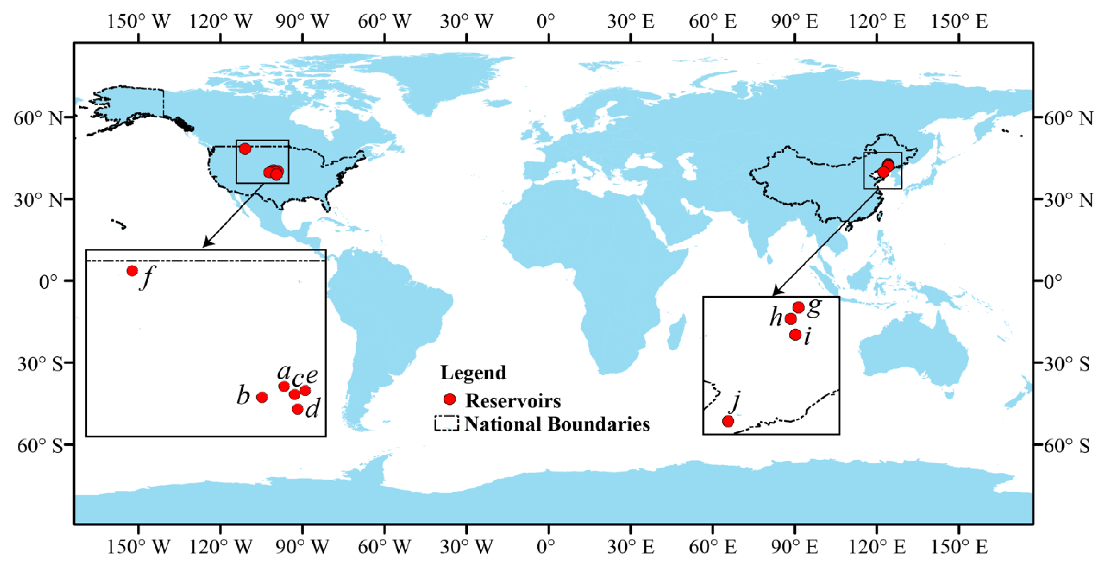
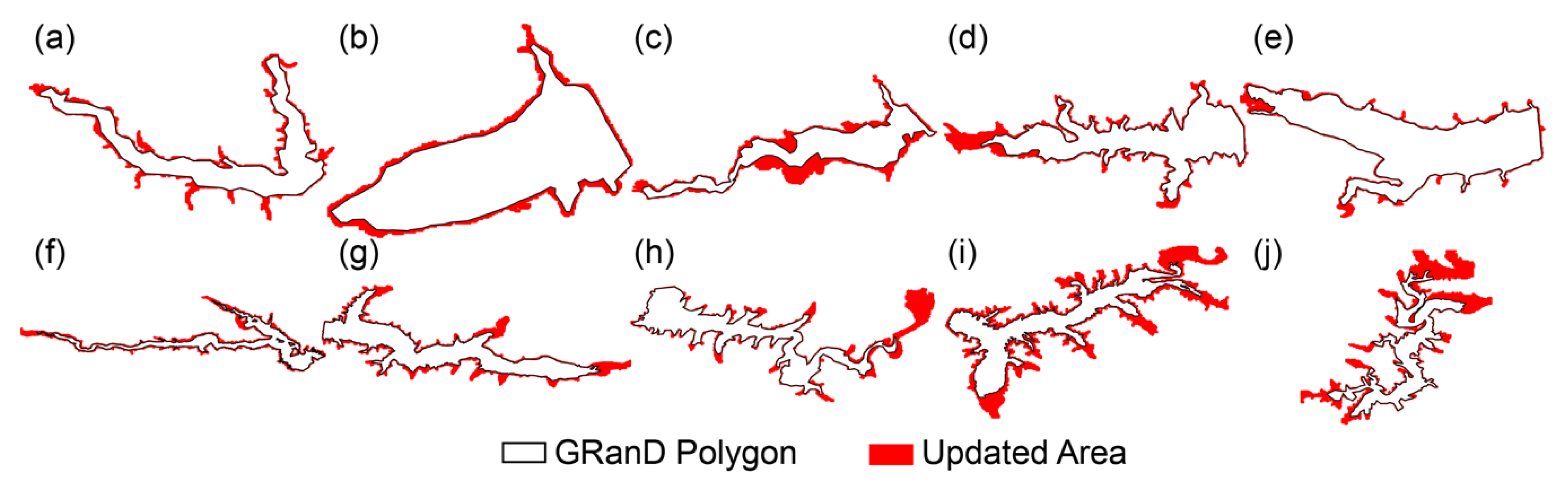
First, the original coverage polygon of each reservoir is obtained from GRanD and extended to where water was once detected by GSW (30 m) during 1984–2015. The locations of the ten selected reservoirs in this study are shown in Figure 1. This procedure is necessary because most polygons from GRanD are delineated from snapshot imagery in the SRTM Water Body Database (SWBD) [30], which could underestimate the extent of the reservoir and the area at capacity by as much as 65% (Figure 2 and Table 1). The updated polygons instead of the original GRanD polygons are used in the study. The areas at capacity, i.e., the maximal coverage areas of reservoirs, is determined by the area of the updated polygons.
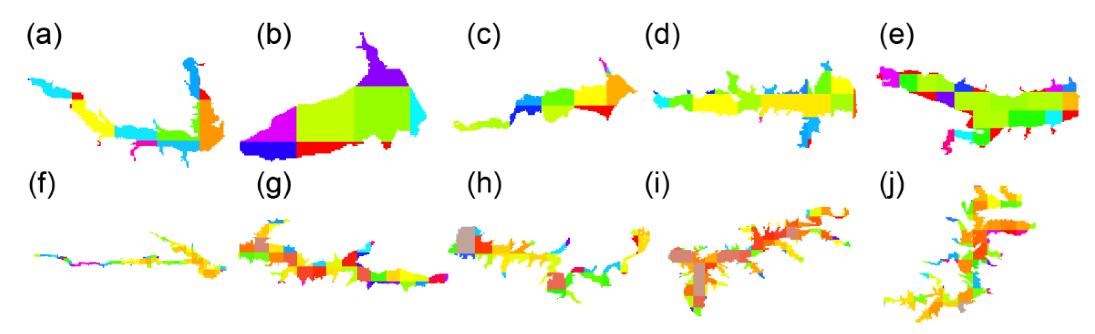
Second, the hypsographic relationship between reservoir surface water areas and the corresponding relative water depths is derived from ETOPO1 for each reservoir. The elevation of each pixel in the reservoir polygon is extracted from ETOPO1, resampled by the nearest neighbor resampling method at 30-m resolution, which is consistent with the resolution of the updated coverage polygons. Figure 3 shows ETOPO1 DEM values with different pixel colors over the ten selected reservoirs. Large reservoirs have denser ETOPO1 values than small reservoirs, which implies the derived curves of large reservoirs are more reliable while those of small reservoirs may suffer from larger uncertainties. The relative water depth of one selected pixel, which represents the water depth in this pixel when all and only the pixels no higher than the selected pixel are fully filled with water, is the elevation of the pixel subtracted by the minimum elevation of the reservoir, and is calculated as:
where is the relative water depth (m), is the elevation value (m) from ETOPO1, and is the minimum of all the elevation values in one reservoir. The corresponding water area of the specific water depth is the sum area of all the pixels no higher than the selected depth and is calculated as:
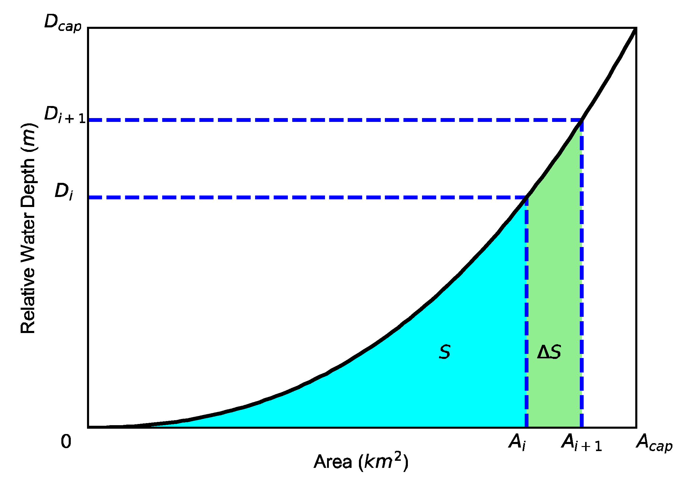
where is the water area corresponding to water depth , is the water area at capacity, is the number of all 30-m pixels in the reservoir, and is the number of all pixels with water depth no higher than . Based on Equation (2), the hypsographic curve of a reservoir can be plotted as the black solid line in Figure 4. We assume the largest water depth over the reservoir exists near the dam, which is observed and recorded as forebay water elevation in reservoirs management.
Third, the cumulative storage is calculated with increasing water area by every one percent of reservoir coverage area and then, the area–storage curve is obtained. The A-S curves derived in this step are referred as uncalibrated curves since they are directly derived from ETOPO1 and not calibrated or constrained by GRanD database. The increased storage , as the light green component (approximate right trapezoid) shown in Figure 4, with water area increasing from to is calculated as:
where I = 0, 1, 2, …, 99. One hundred intervals are found adequate in this study.
The cumulative storage , as the cyan component shown in Figure 4, with water area as is calculated as:
This would be the uncalibrated area–storage curves which suffer great errors mainly originated from the limited absolute vertical accuracy of ETOPO1.
Finally, the area–storage curve is linearly calibrated by the ratio of reported capacity in GRanD over calculated capacity , following:
Relative water depth is defined as the largest water depth over the reservoir when water area is . The reservoir storage could not be directly inferred through D-S curve since no such depth data are conveniently accessible in both remote sensing products and in situ observation records. Therefore, we define a standardized depth–storage curve (SD-S curve) that depicts the relationship between water depth and storage. The storage records can be inferred from SD-S curves with forebay water elevation, which is assumed as the deepest water over the reservoir. The standardized water depth is literally calculated as:
where and are the minimum and maximum of relative water depth values, and ranges from 0 to 1. Combining Equations (5) and (6), the SD-S curve can be obtained as:
The SD-S curves are used to make indirect validation with in situ reservoir storage and forebay elevation records.
3. Results
To evaluate the performance of the proposed method, the derived area–storage (A-S) curves and standardized depth–storage (SD-S) curves of ten reservoirs (reservoirs a-f in the US and g-j in China) are selected to make the validation, where the in situ observation records are available. See characteristics of these 10 reservoirs in Figure 2 and Table 1. The areas at capacity of these selected reservoirs vary from 6 to 82 km2, and the capacity vary from 51 to 2187 million m3, which is larger than the capacity of 93% (6373 of 6862) reservoirs in the GRanD database. This ensures that the validation covers both the small and large reservoirs with various shapes. The coefficient of determination R2 is used to evaluate the performance.
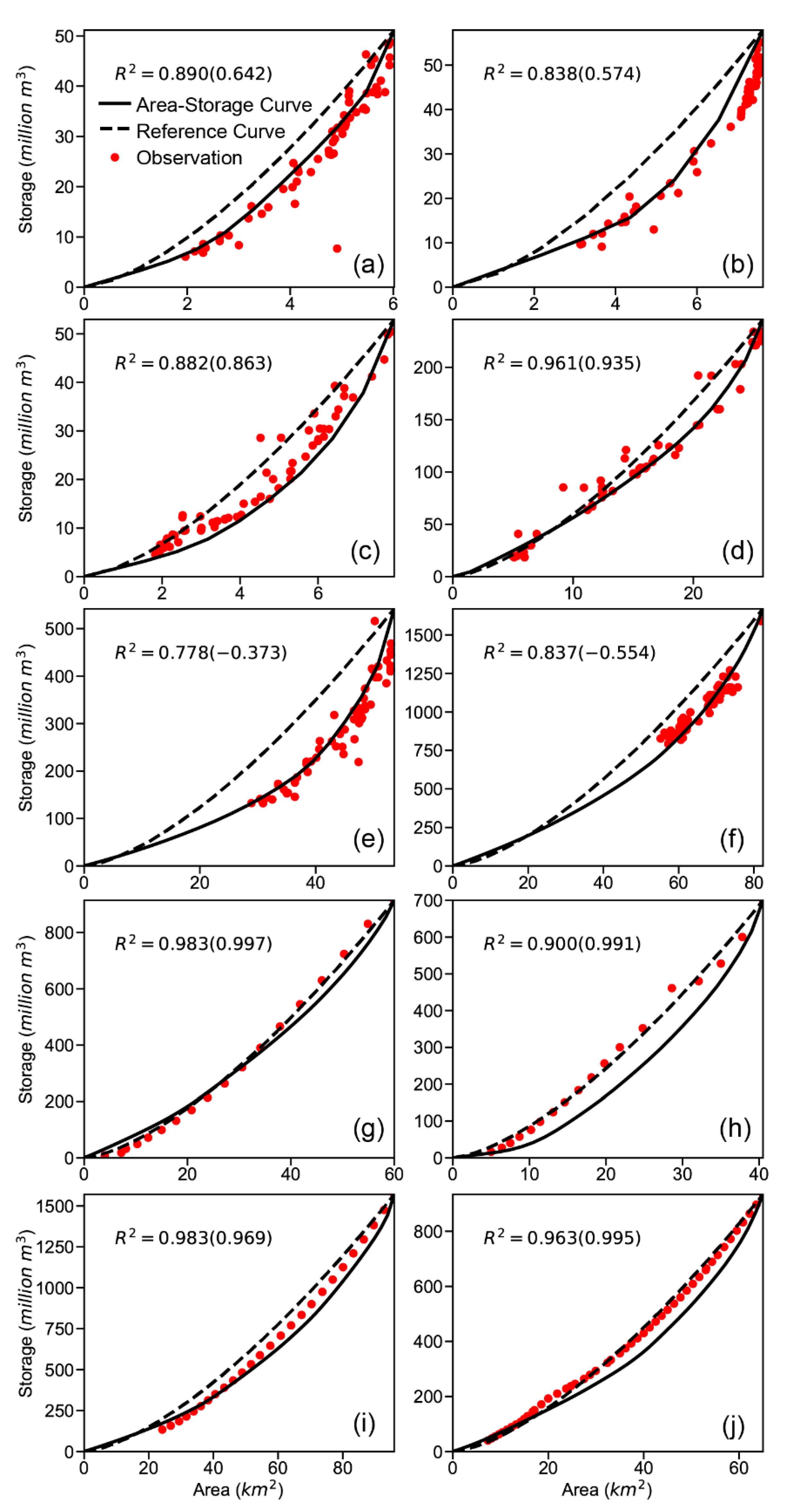
Figure 5 shows the validation of A-S curves of the ten selected reservoirs. The red points in Figure 5a–f represent the observation records of annual maximal or minimal in situ water storage and remote sensed water area during 1984–2015 in the US, while in Figure 5g–j, the red points represent the observed curves of reservoirs collected in China. It can be interpreted from Figure 5 that the derived curves (black solid lines) capture the distribution pattern of red observation points in all 10 reservoirs, with R2 ranging from 0.78 to 0.98. Reference A-S curves from van Bemmelen et al. 2016 [24] (black dashed lines) serve as comparison to show the performance of derived A-S curves in this study. The reference R2 (numbers in brackets in Figure 5) between reference curves and observation records are smaller than our results in Figure 5a–f. This implicates the proposed method in this study performs better in most cases, especially in relatively large reservoirs Figure 5e,f, while the reference curves fail to represent the realistic area–storage relationships probably due to smaller geomorphological similarity around the large reservoirs. The reference curves are derived based on the geomorphological similarity according to van Bemmelen et al. 2016 [24]. Therefore, if a large similarity exits between the existing reservoir and the nearby virtual reservoirs, the A-S relationships of the existing reservoir can be well represented by the reference curves. For a large reservoir, it may be difficult to find nearby virtual reservoirs with large similarity, which may lead to the failed representations of the reference curves. Moreover, the selection of the virtual reservoirs is subjective to expert knowledge and can induce large uncertainties. These two reasons contribute to the large uncertainties of the reference curves in some reservoirs, e.g., in Figure 5e,f. The performances of the two methods are comparable in Figure 5g–j. The derived A-S curves of small reservoirs in Figure 5a–c also show good performance, not limited by the requirement suggested in Zhang and Gao (2016) [16].
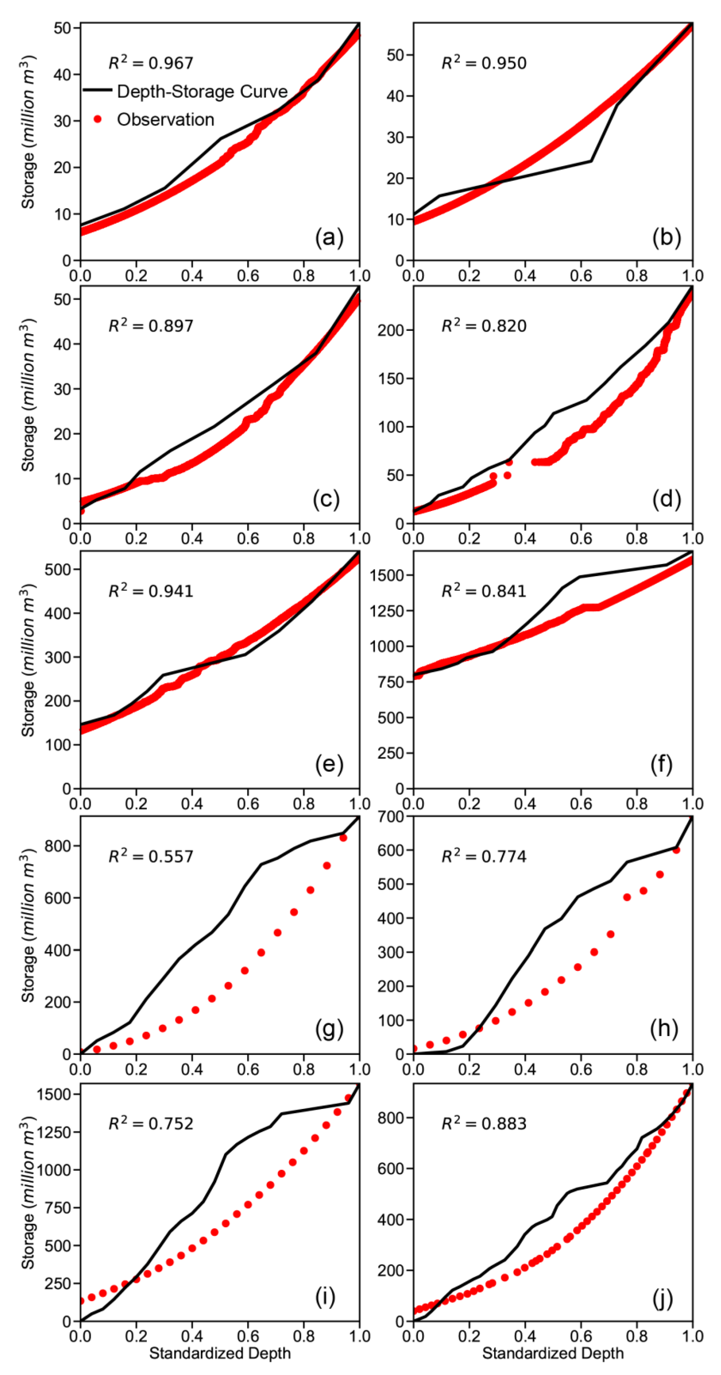
Figure 6 shows the validation of SD-S curves, which serves as the indirect validation of the derived A-S curves. The red points (seem like continuous lines due to large number of points) in the figure represent the daily in situ storage and standardized forebay water elevation records with a few outliers eliminated during 1984–2015 in Figure 6a–f, while in Figure 6g–j the red points represent the observed curves of reservoirs collected in China. We assume as in Section 2 that the forebay region adjacent to the dam has the deepest water over the reservoir. The black SD-S curves capture the distribution pattern of red observation points in nearly all 10 reservoirs, with R2 ranging from 0.56 to 0.97. The SD-S curve and the observation diverge greatly from each other with standardized depth around 0.5–0.7 and converge with each other otherwise. The SD-S curves perform well when the standardized depth (SD) approaches 0 or 1 because the curves are well constrained by the minimal and maximal storage capacities provided by the GRanD database. However, when SD is in the range 0.5–0.7, the curves are less constrained and so a large discrepancy occurs. The scale of the discrepancy varies across different reservoirs depending on the uncertainties of input data and the different shapes of reservoirs. Larger biases are observed in SD-S curves (Figure 6) than in A-S curves (Figure 5). The accuracy of the derived SD-S curves may be improved if the water elevation information over the reservoirs is accessible.
4. Conclusions and Discussion
In this paper, we demonstrate an approach to derive area–storage curves of reservoirs using readily available datasets, i.e., the GRanD database and Landsat-based global surface water extent (GSW) dataset. It should be noted that this approach relies heavily on reservoir storage data archived in the GRanD database and surface water area from the Landsat-based global surface water extent (GSW) data. As no bathymetry or geometric information has been used, it can not only be used at the reservoirs archived in the GRanD database. Despite its limitations, one advantage is that the storage data has highest accuracy because it is from ground observation rather than remote sensing estimates. The validation results suggest that the derived curves can capture the distribution pattern of in situ observation records both in large and small reservoirs in the US and China. The approach shows the potential to be applicable to 80% of global reservoirs (with area at capacity larger than 1 km2; totally occupying 98% capacity of global reservoirs in GRanD) including small ones. This would advance global-scale monitoring and modeling of reservoir storage and area variations. A previous study [31] developed a framework for monitoring hydrological droughts using a global, long-term, monthly, remotely sensed reservoir surface area dataset. The method proposed in this study can be applied to derive the area–storage curve of reservoirs archived in the GRanD database. In addition to reservoir surface area monitoring, it will facilitate global reservoir water storage monitoring using the area–storage curves and remotely sensed reservoir surface area. Furthermore, a new indicator based on reservoir water storage rather than reservoir surface area can be defined for global hydrological drought and water stress monitoring. For global scale studies, the accuracy of the derived area–storage curves should be acceptable, given that most of those curves are not publicly shared. The curves can also be employed in other related fields which use area–storage relationship of reservoirs as an important input, e.g., estimating evaporation over reservoirs [32].
Uncertainties and bias in A-S curves come from three main sources:
- The coverage polygon of each reservoir. The polygon is based on the original GRanD polygon and expanded by the GSW dataset. The uncertainties in both datasets would propagate to affect the real coverage of the reservoir and in result, affect the area at capacity and the topography delineation from ETOPO1.
- The coarse resolution and vertical accuracy of elevation data. The coarse resolution and limited vertical accuracy of the ETOPO1 could cause great uncertainties even errors and restrict its applicability. A finer-resolution (10–60 m) and higher-accuracy (10–25 cm) DEM with water depth information may be derived after SWOT (Surface Water and Ocean Topography mission) [33] to be launched in the year 2021. SWOT would be able to observe lakes with repeated high-resolution elevation measurements, and when combined with high-resolution surface water data, would enable area–storage curves of global lake/reservoirs with better accuracy in the future. For now, however, the proposed approach in this study, which utilizes the readily available ETOPO1, can serve as an alternative approach with satisfied accuracy to provide area–storage curves for the hydrology community. Furthermore, the disadvantages of ETOPO1 are largely compensated in the calibration process by the GRanD and GSW dataset. Although other high-resolution DEMs may have the potential to derive the area–storage curves with some new modified approaches, it is beyond the scope of this study and may be considered and examined in the future.
- The reported capacity in the GRanD database and the sedimentation effect. The calibration in this study heavily depends on , which is collected from multiple unguaranteed sources with various qualities. Moreover, in this study (as well as in previously mentioned studies), the storage capacity of the reservoir is assumed not to change through time and thus, a stationary capacity is adopted, which means the sedimentation effect [34] is not considered and may introduce bias in reservoirs with severe sediment deposition. Basson (2009) [35] reported that the annual reservoir sedimentation rate is about 0.5%–1% of global reservoir storage volume. It means the adding loss of storage is approximately 50 km3 per year worldwide [36]. The highest average reservoir sedimentation rate occurs in arid regions such as the Middle East, Australia, Africa, and western United States [37,38]. Wang and Hu (2009) [39] reported that sedimentation had reduced the reservoir capacity in China by 66%. The previous study also showed that 80% of the useful storage capacity for hydropower production will be lost by 2035, and whereas 70% of the storage volumes used for irrigation will be lost due to sedimentation by 2025 in Asia [40]. As the sediment filling effect is increasingly widespread, many measures have been carried out to preserve reservoir capacity [41,42]. The variation of reservoir storage capacity is difficult to monitor and predict. Wisser et al. (2013) [43] estimated the loss in storage capacity for global large reservoirs from 1901 to 2010, and found that the net reservoir capacity is declining as a result of sedimentation (∼5% compared to the installed capacity). It should be noted that using the fixed reservoir storage capacity in the GRanD database would introduce uncertainty to the area–storage curve estimates. There is an urgent need to update the storage capacity in the database. We also note that the annual change of reservoir capacity is usually small compared to the install capacity. If the storage capacity had been recently updated, the fixed storage capacity may be used to derive the area–storage curve for reservoir water storage monitoring. Local information, e.g., more accurate dynamic capacity of reservoirs, could be used to calibrate the A-S curves on a local scale if higher accuracy is desired. However, for global-scale studies, the proposed approach should work well with acceptable bias.
Author Contributions
Conceptualization, M.M. and Q.T.; Data curation, M.M.; Funding acquisition, Q.T.; Methodology, M.M. and Q.T.; Supervision, Q.T.; Validation, M.M.; Visualization, M.M.; Writing—original draft, M.M.; Writing—review & editing, Q.T., S.H., X.L. and H.C. All authors have read and agreed to the published version of the manuscript.
Funding
This research was funded by the Strategic Priority Research Program of Chinese Academy of Sciences (Grant XDA20060402), the National Natural Science Foundation of China (Grants 41730645 and 41425002), and Newton Advanced Fellowship to Q.T.
Acknowledgments
The updated coverage polygons and the derived area–storage curves of global reservoirs with area at capacity larger than 1 km2 listed in GRanD database are publicly available upon request. We acknowledge the technical assistance from Google Earth Engine (GEE).
Conflicts of Interest
The authors declare no conflict of interest.
References
- Chao, B.F.; Wu, Y.H.; Li, Y.S. Impact of Artificial Reservoir Water Impoundment on Global Sea Level. Science 2008, 320, 212–214. [Google Scholar] [CrossRef] [Green Version]
- Döll, P.; Fiedler, K.; Zhang, J. Global-scale analysis of river flow alterations due to water withdrawals and reservoirs. Hydrol. Earth Syst. Sci. 2009, 13, 2413–2432. [Google Scholar] [CrossRef] [Green Version]
- Zhou, T.; Nijssen, B.; Gao, H.; Lettenmaier, D.P. The Contribution of Reservoirs to Global Land Surface Water Storage Variations. J. Hydrometeorol. 2016, 17, 309–325. [Google Scholar] [CrossRef]
- Hanasaki, N.; Kanae, S.; Oki, T. A reservoir operation scheme for global river routing models. J. Hydrol. 2006, 327, 22–41. [Google Scholar] [CrossRef]
- Hanasaki, N.; Kanae, S.; Oki, T.; Masuda, K.; Motoya, K.; Shirakawa, N.; Shen, Y.; Tanaka, K. An integrated model for the assessment of global water resources—Part 1: Model description and input meteorological forcing. Hydrol. Earth Syst. Sci. 2008, 12, 1007–1025. [Google Scholar] [CrossRef] [Green Version]
- Wisser, D.; Fekete, B.M.; Vörösmarty, C.J.; Schumann, A.H. Reconstructing 20th century global hydrography: A contribution to the Global Terrestrial Network-Hydrology (GTN-H). Hydrol. Earth Syst. Sci. 2010, 14, 1–24. [Google Scholar] [CrossRef] [Green Version]
- Pokhrel, Y.; Hanasaki, N.; Koirala, S.; Cho, J.; Yeh, P.J.-F.; Kim, H.; Kanae, S.; Oki, T. Incorporating Anthropogenic Water Regulation Modules into a Land Surface Model. J. Hydrometeorol. 2012, 13, 255–269. [Google Scholar] [CrossRef] [Green Version]
- Voisin, N.; Liu, L.; Hejazi, M.; Tesfa, T.; Li, H.; Huang, M.; Liu, Y.; Leung, L.R. One-Way coupling of an integrated assessment model and a water resources model: Evaluation and implications of future changes over the US Midwest. Hydrol. Earth Syst. Sci. 2013, 17, 4555–4575. [Google Scholar] [CrossRef] [Green Version]
- Biemans, H.; Haddeland, I.; Kabat, P.; Ludwig, F.; Hutjes, R.W.A.; Heinke, J.; Von Bloh, W.; Gerten, D. Impact of reservoirs on river discharge and irrigation water supply during the 20th century. Water Resour. Res. 2011, 47, 1–15. [Google Scholar] [CrossRef] [Green Version]
- Liu, X.; Tang, Q.; Voisin, N.; Cui, H. Projected impacts of climate change on hydropower potential in China. Hydrol. Earth Syst. Sci. 2016, 20, 3343–3359. [Google Scholar] [CrossRef] [Green Version]
- Nazemi, A.; Wheater, H.S. On inclusion of water resource management in Earth system models—Part 2: Representation of water supply and allocation and opportunities for improved modeling. Hydrol. Earth Syst. Sci. 2015, 19, 63–90. [Google Scholar] [CrossRef] [Green Version]
- Gao, H.; Birkett, C.; Lettenmaier, D.P. Global monitoring of large reservoir storage from satellite remote sensing. Water Resour. Res. 2012, 48, 1–12. [Google Scholar] [CrossRef] [Green Version]
- Zhang, S.; Gao, H.; Naz, B.S. Monitoring reservoir storage in South Asia frommultisatellite remote sensing. Water Resour. Res. 2014, 50, 8927–8943. [Google Scholar] [CrossRef]
- Gao, H. Satellite remote sensing of large lakes and reservoirs: From elevation and area to storage. Wiley Interdiscip. Rev. Water 2015, 2, 147–157. [Google Scholar] [CrossRef]
- Crétaux, J.F.; Biancamaria, S.; Arsen, A.; Bergé-Nguyen, M.; Becker, M. Global surveys of reservoirs and lakes from satellites and regional application to the Syrdarya river basin. Environ. Res. Lett. 2015, 10, 015002. [Google Scholar] [CrossRef] [Green Version]
- Zhang, S.; Gao, H. A novel algorithm for monitoring reservoirs under all-weather conditions at a high temporal resolution through passive microwave remote sensing. Geophys. Res. Lett. 2016, 43, 8052–8059. [Google Scholar] [CrossRef]
- Lehner, B.; Liermann, C.R.; Revenga, C.; Vörömsmarty, C.; Fekete, B.; Crouzet, P.; Döll, P.; Endejan, M.; Frenken, K.; Magome, J.; et al. High-resolution mapping of the world’s reservoirs and dams for sustainable river-flow management. Front. Ecol. Environ. 2011, 9, 494–502. [Google Scholar] [CrossRef] [Green Version]
- G-REALM: A Lake/Reservoir Monitoring Tool for Water Resources and Regional Security Assessment. Available online: https://www.pecad.fas.usda.gov/cropexplorer/global_reservoir (accessed on 1 July 2017).
- Crétaux, J.F.; Jelinski, W.; Calmant, S.; Kouraev, A.; Vuglinski, V.; Bergé-Nguyen, M.; Gennero, M.C.; Nino, F.; Abarca Del Rio, R.; Cazenave, A.; et al. SOLS: A lake database to monitor in the Near Real Time water level and storage variations from remote sensing data. Adv. Space Res. 2011, 47, 1497–1507. [Google Scholar] [CrossRef]
- Liebe, J.; van de Giesen, N.; Andreini, M. Estimation of small reservoir storage capacities in a semi-arid environment. Phys. Chem. Earth 2005, 30, 448–454. [Google Scholar] [CrossRef]
- Sawunyama, T.; Senzanje, A.; Mhizha, A. Estimation of small reservoir storage capacities in Limpopo River Basin using geographical information systems (GIS) and remotely sensed surface areas: Case of Mzingwane catchment. Phys. Chem. Earth 2006, 31, 935–943. [Google Scholar] [CrossRef]
- Klein, I.; Gessner, U.; Dietz, A.J.; Kuenzer, C. Global WaterPack—A 250 m resolution dataset revealing the daily dynamics of global inland water bodies. Remote Sens. Environ. 2017, 198, 345–362. [Google Scholar] [CrossRef]
- Pekel, J.-F.; Cottam, A.; Gorelick, N.; Belward, A.S. High-resolution mapping of global surface water and its long-term changes. Nature 2016, 540, 418–422. [Google Scholar] [CrossRef] [PubMed]
- Van Bemmelen, C.W.T.; Mann, M.; de Ridder, M.P.; Rutten, M.M.; van de Giesen, N.C. Determining water reservoir characteristics with global elevation data. Geophys. Res. Lett. 2016, 43, 11278–11286. [Google Scholar] [CrossRef] [Green Version]
- Amante, C.; Eakins, B.W. ETOPO1 1 Arc-Minute Global Relief Model: Procedures, Data Sources and Analysis; NOAA Technical Memorandum NESDIS NGDC-24; National Geophysical Data Center, NOAA, 2009; p. 19. Available online: http://www.ngdc.noaa.gov/mgg/global/global.html (accessed on 1 June 2017).
- Yamazaki, D.; Ikeshima, D.; Tawatari, R.; Yamaguchi, T.; O’Loughlin, F.; Neal, J.C.; Sampson, C.C.; Kanae, S.; Bates, P.D. A high accuracy map of global terrain elevations. Geophys. Res. Lett. 2017, 44, 5844–5853. [Google Scholar] [CrossRef] [Green Version]
- USBR US Bureau of Reclamation. Available online: https://www.usbr.gov/ (accessed on 1 June 2017).
- Li, Y.; Zhang, C.; Chu, J.; Cai, X.; Zhou, H. Reservoir Operation with Combined Natural Inflow and Controlled Inflow through Interbasin Transfer: Biliu Reservoir in Northeastern China. J. Water Resour. Plan. Manag. 2015, 142, 05015009. [Google Scholar] [CrossRef]
- Zhang, C.; Li, Y.; Chu, J.; Fu, G.; Tang, R.; Qi, W. Use of Many-Objective Visual Analytics to Analyze Water Supply Objective Trade-Offs with Water Transfer. J. Water Resour. Plan. Manag. 2017, 143, 05017006. [Google Scholar] [CrossRef] [Green Version]
- NASA/NGA SRTM Water Body Data Product Specific Guidance, Version 2.0. Available online: http://dds.cr.usgs.gov/srtm/version2_1/SWBD/SWBD_Documentation/ (accessed on 1 June 2017).
- Zhao, G.; Gao, H. Towards Global Hydrological Drought Monitoring Using Remotely Sensed Reservoir Surface Area. Geophys. Res. Lett. 2019, 46, 13027–13035. [Google Scholar] [CrossRef]
- Zhang, C.; Ding, W.; Li, Y.; Tang, Y.; Wang, D. Catchments’ hedging strategy on evapotranspiration for climatic variability. Water Resour. Res. 2016, 52, 9036–9045. [Google Scholar] [CrossRef]
- Biancamaria, S.; Lettenmaier, D.P.; Pavelsky, T.M. The SWOT Mission and Its Capabilities for Land Hydrology. Surv. Geophys. 2016, 37, 307–337. [Google Scholar] [CrossRef] [Green Version]
- Dargahi, B. Reservoir Sedimentation. In Encyclopedia of Lakes and Reservoirs; Bengtsson, L., Herschy, R.W., Fairbridge, R.W., Eds.; Springer: Dordrecht, The Netherlands, 2012; pp. 628–649. [Google Scholar]
- Basson, G. Management of siltation in existing and new reservoirs. In Proceedings of the 23rd Congress of the International Commission on Large Dams ICOLD CIGB, Basilia, Brazil, 25–29 May 2009. [Google Scholar]
- Palmieri, A.; Shah, F.; Annandale, G.; Dinar, A. Reservoir Conservation Volume I: The RESCON Approach; World Bank: Washington, DC, USA, 2003; Available online: http://documents.worldbank.org/curated/en/819541468138875126/RESCON-approach (accessed on 20 February 2020).
- Graf, W.L.; Wohl, E.; Sinha, T.; Sabo, J.L. Sedimentation and sustainability of western American reservoirs. Water Resour. Res. 2010, 46, 1–34. [Google Scholar] [CrossRef]
- George, M.W.; Hotchkiss, R.H.; Huffaker, R. Reservoir sustainability and sediment management. J. Water Resour. Plan. Manag. 2017, 143, 04016077. [Google Scholar] [CrossRef] [Green Version]
- Wang, Z.; Hu, C. Strategies for managing reservoir sedimentation. Int. J. Sediment Res. 2009, 24, 369–384. [Google Scholar] [CrossRef]
- Schleiss, A.J.; Franca, M.J.; Juez, C.; De Cesare, G. Reservoir sedimentation. J. Hydraul. Res. 2016, 54, 595–614. [Google Scholar] [CrossRef]
- Kondolf, G.M.; Gao, Y.; Annandale, G.W.; Morris, G.L.; Jiang, E.; Zhang, J.; Cao, Y.; Carling, P.; Fu, K.; Guo, Q.; et al. Sustainable sediment management in reservoirs and regulated rivers: Experiences from five continents. Earth’s Future 2014, 2, 256–280. [Google Scholar] [CrossRef]
- Espa, P.; Batalla, R.J.; Brignoli, M.L.; Crosa, G.; Gentili, G.; Quadroni, S. Tackling reservoir siltation by controlled sediment flushing: Impact on downstream fauna and related management issues. PLoS ONE 2019, 14, e0218822. [Google Scholar] [CrossRef]
- Wisser, D.; Frolking, S.; Hagen, S.; Bierkens, M.F.P. Beyond peak reservoir storage? A global estimate of declining water storage capacity in large reservoirs. Water Resour. Res. 2013, 49, 5732–5739. [Google Scholar] [CrossRef] [Green Version]
Figure 1.
The locations of the ten selected reservoirs used in the study. (a) Hugh Butler Lake; (b) Bonny Reservoir; (c) Keith Sebelius Lake; (d) Cedar Bluff Reservoir; (e) Harlan County Lake; (f) Lake Elwell; (g) Qinghe Reservoir; (h) Chaihe Reservoir; (i) Dahuofang Reservoir; (j) Biliuhe Reservoir.

Figure 2.
Original reservoir polygons in the GRanD (Global Reservoir and Dam) database and updated polygons of the ten selected reservoirs. Reservoir polygons are scaled to the similar length for plotting convenience, so the sizes of polygons in the figure do not represent the real coverage area (see Table 1). (a) Hugh Butler Lake; (b) Bonny Reservoir; (c) Keith Sebelius Lake; (d) Cedar Bluff Reservoir; (e) Harlan County Lake; (f) Lake Elwell; (g) Qinghe Reservoir; (h) Chaihe Reservoir; (i) Dahuofang Reservoir; (j) Biliuhe Reservoir.

Figure 3.
ETOPO1 DEM values with different pixel colors over the ten selected reservoirs. (a) Hugh Butler Lake; (b) Bonny Reservoir; (c) Keith Sebelius Lake; (d) Cedar Bluff Reservoir; (e) Harlan County Lake; (f) Lake Elwell; (g) Qinghe Reservoir; (h) Chaihe Reservoir; (i) Dahuofang Reservoir; (j) Biliuhe Reservoir.

Figure 4.
Hypsographic curve representation of a reservoir. is the increased storage with water area increasing from to and water depth increasing from to . is the cumulative reservoir storage with water area as . and are respectively the area at capacity and the depth at capacity.
Figure 4.
Hypsographic curve representation of a reservoir. is the increased storage with water area increasing from to and water depth increasing from to . is the cumulative reservoir storage with water area as . and are respectively the area at capacity and the depth at capacity.

Figure 5.
Area–storage curves and their validation results of the ten selected reservoirs: (a) Hugh Butler Lake; (b) Bonny Reservoir; (c) Keith Sebelius Lake; (d) Cedar Bluff Reservoir; (e) Harlan County Lake; (f) Lake Elwell; (g) Qinghe Reservoir; (h) Chaihe Reservoir; (i) Dahuofang Reservoir; (j) Biliuhe Reservoir. Area–storage curves (black solid lines) are derived by the proposed method in this study. Reference curves (black dashed lines) represent the A-S curves in van Bemmelen et al. 2016 [24]. Red points in (a–f) represent the annual maximum and minimum of in situ storage records and remote sensed water area estimates during 1984–2015 in US. Red points in (g–j) represent the observed curves in China.

Figure 6.
Standardized depth–storage curves and their validation results of the ten selected reservoirs: (a) Hugh Butler Lake; (b) Bonny Reservoir; (c) Keith Sebelius Lake; (d) Cedar Bluff Reservoir; (e) Harlan County Lake; (f) Lake Elwell; (g) Qinghe Reservoir; (h) Chaihe Reservoir; (i) Dahuofang Reservoir; (j) Biliuhe Reservoir. Red points in (a–f) represent the daily in situ storage and forebay water elevation records with a few outliers (which contains normal water elevation data but with extremely large water storage data) eliminated during 1984–2015 in US. Red points in (g–j) represent the observed curves in China. Water surface elevation and relative water depth are standardized for validation convenience between the derived curves and the in situ records, following respectively: and .


Table 1.
Characteristics of the ten selected reservoirs in this study.
| ID in Figures | GRanD ID | Reservoir Name | Capacity (million m3) | Area at Capacity (km2) | GRanD Area (km2) | Updated Area Ratio (%) |
|---|---|---|---|---|---|---|
| a | 939 | Hugh Butler Lake | 51.1 | 6.0 | 5.0 | 20% |
| b | 958 | Bonny Reservoir | 57.9 | 7.6 | 6.8 | 12% |
| c | 953 | Keith Sebelius Lake | 52.9 | 8.0 | 5.7 | 39% |
| d | 976 | Cedar Bluff Reservoir | 245.7 | 25.8 | 21.2 | 22% |
| e | 948 | Harlan County Lake | 541.8 | 53.6 | 50.0 | 7% |
| f | 300 | Lake Elwell | 1669.5 | 82.4 | 65.2 | 26% |
| g | 5855 | Qinghe Reservoir | 971.0 | 46.1 | 37.1 | 24% |
| h | 5864 | Chaihe Reservoir | 650.0 | 26.2 | 20.8 | 26% |
| i | 5873 | Dahuofang Reservoir | 2187.0 | 79.8 | 51.1 | 56% |
| j | 5913 | Biliuhe Reservoir | 930.0 | 53.2 | 32.2 | 65% |
© 2020 by the authors. Licensee MDPI, Basel, Switzerland. This article is an open access article distributed under the terms and conditions of the Creative Commons Attribution (CC BY) license (http://creativecommons.org/licenses/by/4.0/).
Share and Cite
MDPI and ACS Style
Mu, M.; Tang, Q.; Han, S.; Liu, X.; Cui, H. Using GRanD Database and Surface Water Data to Constrain Area–Storage Curve of Reservoirs. Water 2020, 12, 1242. https://doi.org/10.3390/w12051242
AMA Style
Mu M, Tang Q, Han S, Liu X, Cui H. Using GRanD Database and Surface Water Data to Constrain Area–Storage Curve of Reservoirs. Water. 2020; 12(5):1242. https://doi.org/10.3390/w12051242
Chicago/Turabian StyleMu, Mengfei, Qiuhong Tang, Songjun Han, Xiaomang Liu, and Huijuan Cui. 2020. "Using GRanD Database and Surface Water Data to Constrain Area–Storage Curve of Reservoirs" Water 12, no. 5: 1242. https://doi.org/10.3390/w12051242
Note that from the first issue of 2016, this journal uses article numbers instead of page numbers. See further details here.