Potential Fields in Fluid Mechanics: A Review of Two Classical Approaches and Related Recent Advances

Abstract

The use of potential fields in fluid dynamics is retraced, ranging from classical potential theory to recent developments in this evergreen research field. The focus is centred on two major approaches and their advancements: (i) the Clebsch transformation and (ii) the classical complex variable method utilising Airy’s stress function, which can be generalised to a first integral methodology based on the introduction of a tensor potential and parallels drawn with Maxwell’s theory. Basic questions relating to the existence and gauge freedoms of the potential fields and the satisfaction of the boundary conditions required for closure are addressed; with respect to (i), the properties of self-adjointness and Galilean invariance are of particular interest. The application and use of both approaches is explored through the solution of four purposely selected problems; three of which are tractable analytically, the fourth requiring a numerical solution. In all cases, the results obtained are found to be in excellent agreement with corresponding solutions available in the open literature.

1. Introduction

In various branches of physics, potentials continue to be used as additional auxiliary fields for the advantageous reformulation of one or more governing equations. Classical electrodynamics serves as a prime illustrative example of their use [1], enabling Maxwell equations in their commonly expressed form, comprised of two scalar and two vector equations for the two observables—electric field $\overrightarrow{E}$ and magnetic flux density $\overrightarrow{B}$—to be formulated differently in terms of the derivatives of a scalar potential $\phi$ and a vector potential $\overrightarrow{A}$, such that $\overrightarrow{E}=-\nabla \phi -{\partial }_t\overrightarrow{A}$ and $\overrightarrow{B}=\nabla \times \overrightarrow{A}$, respectively; in which case, two of the four Maxwell equations are fulfilled identically while the other two form a self-adjoint pair—i.e., can be obtained from a variational principle. Moreover, followed by proper gauging of the potential fields, a fully decoupled form of Maxwell’s equations in terms of two inhomogeneous d’Alembert equations is obtained. From a mathematical viewpoint, amendments to the original equations comprise:

• A reduction in the number of equations and unknowns;
• Self-adjointness of the equations;
• A full decoupling of the equations;
• Transformation of the equations to a known mathematical type.

Despite the above benefits, a historical debate reaching back to Heaviside [2,3] has surrounded the Maxwell potentials and their rationale, which were not free of polemics [4,5,6]. A major objection against the use of potential fields has surrounded their mathematical non-uniqueness, implying that they are not observable by physical measurements. In the case of the Maxwell potentials, the transformation

$$\begin{array}{cc}\hfill \overrightarrow{A}\to {\overrightarrow{A}}^{\prime }& =\overrightarrow{A}+\nabla \chi \hfill \end{array}$$

(1)

$$\begin{array}{cc}\hfill \phi \to {\phi }^{\prime }& =\phi -{\partial }_t\chi \hfill \end{array}$$

(2)

in terms of an arbitrary scalar field $\chi$ defines an alternative set of potentials related identically to the observable fields $\overrightarrow{E}$ and $\overrightarrow{B}$. The non-uniqueness of the original Maxwell potentials does not reflect a weak point in the theory; on the contrary, it defines a symmetry that has proven formative in the usage of potential fields in modern theoretical physics as well as ground-breaking with respect to the subsequent development of gauge theory [7]. Each of which confirm Maxwell’s theory to be a significant reference point for other field theories, an obvious example being the potential representation of the Weyl tensor in general relativity [8,9].

Subsequently, based on the publications of Ehrenberg and Siday [10], Aharonov and Bohm [11], the so-called Aharonov–Bohm solenoid effect—which takes place when the wave function of a charged particle passes around a long solenoid and experiences a phase shift as a result of the enclosed magnetic field, despite the magnetic field being negligible outside the solenoid—gave rise to a second debate concerning the physical meaning of the vector Potential $\overrightarrow{A}$. This effect is frequently misunderstood: it does not allow for a point-wise “measurement” of $\overrightarrow{A}$ since only the integral magnetic flux can be determined from the phase shift, while the gauge transformation in Equation (1) is still a symmetry of the Schrödinger–Maxwell theory predicting the effect properly; thus any gradient field $\nabla \chi$ can be added to the vector potential $\overrightarrow{A}$ leading to the same experimental result. Nevertheless, the question still remains an open one as to what physical role the vector potential plays and controversy surrounding it persists; see, for example, [12,13,14,15,16,17,18].

In summary, the use of potentials is motivated from both a mathematical and physical viewpoint: mathematically the original equations can be manipulated in beneficial ways, while physically new insight concerning the structure of the theory is provided via the reformulated equation set. Both of these aspects are considered subsequently.

The particular aim henceforth is to demonstrate the application of potential methods to fluid mechanics. As is well known in the case of an incompressible inviscid irrotational fluid flow, by expressing the velocity field $\overrightarrow{v}$ in terms of a scalar potential $\phi$:

$$\overrightarrow{v}=\nabla \phi$$

(3)

the associated equations of motion are reduced to Bernoulli’s equation, resulting as a first integral of Euler’s equations together with a Laplace equation

$${\nabla }^2\phi =0$$

(4)

for the potential via the continuity equation. Since Bernoulli’s equation is essentially the conditional equation for the pressure field, only Equation (4) remains to be solved, elevating potential flow theory to the status of an essential topic in standard fluid dynamics text books [19,20,21,22]. Despite the obvious advantage of making various flow problems more tractable, the approach is restricted to inviscid and irrotational barotropic flows. In order to extend the methodology to encompass a wider range of flow problems, generalisations of and alternatives to Equation (3) have emerged. Of these, the following two major strands only are explored in the present work:

• The so-called Clebsch transformation [19,20,23] and related methodologies enabling, in the first instance, Euler’s equation to be reformulated as a generalised Bernoulli equation complemented with two transport equations for the Clebsch potentials. The approach was subsequently generalised to encompass baroclinic flow by Seliger and Witham [24], but still with the restriction that the flow is inviscid and heat conduction absent. Note that the Clebsch transformation has been applied to physical problems beyond fluid mechanics including Maxwell theory in classical electrodynamics [25], the field of Magnetohydrodynamics [26], relativistic dynamical systems [27] and even in relation to quantum theory within the context of (a) the quantisation of vortex tubes Madelung [28], Schoenberg [29], (b) generalised membranes [30] and (c) relativistic quantum vorticity [31].
• The complex variable method, developed in the first half of the 20th century and originally related to problems in plane linear elasticity [32,33]. The method was subsequently adopted by the fluid mechanics community: in the case of 2D Stokes flow ($\mathrm{Re}\to 0$) it has led to solutions based on a complex-valued Goursat representation of the stream function in terms of two analytic functions, which has been generalised incrementally, starting with Legendre [34] and followed by Coleman [35], Ranger [36], and Scholle et al. [37], Marner et al. [38], resulting finally in an exact complex-valued first integral of the 2D unsteady NS equations, based on the introduction of an auxiliary potential field. A further generalisation to 3D viscous flow has been achieved only recently using a tensor potential in place of the complex potential field employed in two-dimensions [39].

Historically, both approaches have been subject to limitations on their usage: the Clebsch transformation originated for the case of inviscid flow ($\mathrm{Re}\to \infty$) and the complex variable method for that of 2D Stokes flow ($\mathrm{Re}\to 0$). Recent advancements have lifted these restrictions. In this review, the origin and evolution of both methods is retraced and potential future developments highlighted. Section 2 considers the Clebsch transformation, starting from its origins in inviscid barotropic flow theory, Section 2.1. After commenting on the global existence of the Clebsch variables, Section 2.2, it is demonstrated via a rigorous symmetry analysis, Section 2.2, that the Clebsch representation of the velocity is a natural outcome of Galilean invariance via Noether’s theorem. An extended Clebsch transformation for viscous flow is then presented in Section 2.3 and followed, Section 2.4, by applying it to the problem of viscous stagnation flow. The complex variable method and its progression to a tensor potential approach is outlined in Section 3, beginning in Section 3.1 with the use of Airy’s stress function with respect to steady-state equilibrium conditions for an arbitrary continuum in general and for Stokes’s flow in particular. In Section 3.2, the approach is generalised to encompass the full unsteady 2D-NS equations, utilising a complex potential. A serendipitous benefit is that of enabling the integration of the dynamic boundary condition along a free surface, or interface, and its reduction to a standard form, as shown in Section 3.3, as subsequently utilised in Section 3.4 for the numerical solution of a free surface film flow problem. Latterly, a particularly noteworthy advance, Section 3.5, has been that of overcoming the 2D restriction. This has been achieved by rearranging the complex equations in a tensor form leading to a potential-based first integral of the full 3D-NS equations with a seamless extension to an analogous form of the 4D relativistic energy momentum equations. Concluding remarks are provided in Section 4.

Finally, it would be remiss and incomplete not to point out that in the field of fluid mechanics other approaches to the use of potentials for solving the equations of motion exist that have not been considered in the present text. In this sense and as instructive examples, the reader is referred to the work of Papkovich and Neuber [40], Lee et al. [41], Greengard and Jiang [42].

2. Clebsch Transformation Approach

2.1. The Clebsch Transformation for Inviscid Flows

For inviscid flow, Clebsch [19,20,23] proposed a non-standard potential representation for the velocity field, in terms of the so-called Clebsch variables $\phi ,\alpha ,\beta$, of the form:

$$\overrightarrow{u}=\nabla \phi +\alpha \nabla \beta .$$

(5)

From a mathematical viewpoint, the potential representation in Equation (5) is a decomposition of the velocity field into a curl-free part $\nabla \phi$ and a helicity-free part $\alpha \nabla \beta$. Schoenberg [29] has shown that the above decomposition is not unique; by applying the gauge transformation:

$$\begin{array}{ccc}\hfill \phi ⟶& {\phi }^{\prime }& =\phi +f(\alpha ,\beta ,t)\hfill \\ \hfill \alpha ⟶& {\alpha }^{\prime }& =g(\alpha ,\beta ,t)\hfill \\ \hfill \beta ⟶& {\beta }^{\prime }& =h(\alpha ,\beta ,t)\hfill \end{array}$$

(6)

an equivalent set of Clebsch variables ${\phi }^{\prime },{\alpha }^{\prime },{\beta }^{\prime }$ is given if and only if the functions $f,g,h$ fulfil the following two PDEs:

$$\begin{array}{ccc}\hfill \frac{\partial f}{\partial \beta }+g\frac{\partial h}{\partial \beta }& =& \alpha ,\hfill \end{array}$$

(7)

$$\begin{array}{ccc}\hfill \frac{\partial f}{\partial \alpha }+g\frac{\partial h}{\partial \alpha }& =& 0.\hfill \end{array}$$

(8)

By applying Equation (5) to Euler’s equations for inviscid flows, one obtains:

$$\overrightarrow{0}=\frac{\mathrm{D}\overrightarrow{u}}{\mathrm{D}t}+\nabla [P+U]=\nabla \left[\frac{\partial \phi }{\partial t}+\alpha \frac{\partial \beta }{\partial t}+\frac{\overrightarrow{u}{}^2}{2}+P\left(\varrho \right)+U\right]+\frac{\mathrm{D}\alpha }{\mathrm{D}t}\nabla \beta -\frac{\mathrm{D}\beta }{\mathrm{D}t}\nabla \alpha ,$$

(9)

with the pressure function $P\left(\varrho \right)=\int {\varrho }^{-1}\mathrm{d}p$ and U the specific potential energy of the external force. The operator $\mathrm{D}/\mathrm{D}t=\partial /\partial t+\overrightarrow{u}·\nabla$ is the material time derivative. Being basically of the form:

$$\nabla \left[\cdots \right]+\left[\cdots \right]\nabla \alpha +\left[\cdots \right]\nabla \beta =\overrightarrow{0},$$

(10)

this vector equation can be decomposed according to:

$$\begin{array}{ccc}\hfill \frac{\partial \phi }{\partial t}+\alpha \frac{\partial \beta }{\partial t}+\frac{\overrightarrow{u}{}^2}{2}+P+U& =& F(\alpha ,\beta ,t),\hfill \end{array}$$

(11)

$$\begin{array}{ccc}\hfill \frac{\mathrm{D}\alpha }{\mathrm{D}t}& =& -\frac{\partial F}{\partial \beta },\hfill \end{array}$$

(12)

$$\begin{array}{ccc}\hfill \frac{\mathrm{D}\beta }{\mathrm{D}t}& =& \frac{\partial F}{\partial \alpha },\hfill \end{array}$$

(13)

containing an unknown function $F(\alpha ,\beta ,t)$; which, making use of the gauge transformation of Equation (6), leads to $F\to 0$. The above three scalar field equations represent a first integral of Euler’s equations and are self-adjoint. However, their most intriguing feature is that the vorticity:

$$\overrightarrow{\omega }=\frac{1}{2}\nabla \times \overrightarrow{u}=\frac{1}{2}\nabla \alpha \times \nabla \beta ,$$

(14)

is given by the two scalar fields $\alpha ,\beta$, only. Hence, the vortex dynamics is reduced to and conveniently captured by the two transport Equations (12) and (13). This beneficial feature has been exploited by, for example, Prakash et al. [43], who utilised the Clebsch transformation as a generalisation of classical potential theory for the simulation of bubble dynamics.

Another beneficial feature of the transformed field equations is their self-adjointness: they result from a variational principle:

$$\delta \underset{t_1}{\overset{t_2}{\int }}\underset{V}{\int \int \int }\ell \left(\varrho ,\alpha ,\partial \phi ,\partial \beta ,\overrightarrow{x},t\right)\mathrm{d}V\mathrm{d}t=0,$$

(15)

with respect to free and independent variation of the four fields $\varrho ,\phi ,\alpha ,\beta$ and their first order spatial and temporal derivatives for fixed values at initial and final time, $t_{1,2}$, with the Lagrangian given as [25]:

$$\ell \left(\varrho ,\alpha ,\partial \phi ,\partial \beta ,\overrightarrow{x},t\right)=-\varrho \left[\frac{\partial \phi }{\partial t}+\alpha \frac{\partial \beta }{\partial t}+\frac{1}{2}{\left(\nabla \phi +\alpha \nabla \beta \right)}^2+e\left(\varrho \right)+U\left(\overrightarrow{x},t\right)\right],$$

(16)

for the specific elastic energy $e\left(\varrho \right)$ fulfilling $e\left(\varrho \right)+\varrho e^{\prime }\left(\varrho \right)=P\left(\varrho \right)$. For generalisations of the above variational principle toward thermal degrees of freedom, reference is made to [24,44,45,46].

2.2. A Note on the Global Existence of the Clebsch Variables

When introducing potentials as auxiliary fields, their existence has to be clarified first. Referring to the classical example $\overrightarrow{u}=\nabla \phi$ from potential theory corresponding to the special case of the Clebsch representation in Equation (5) with $\alpha =\beta =0$, it is obvious that it applies only to vortex-free fields, i.e., $\nabla \times \overrightarrow{u}=\overrightarrow{0}$. However, according to Equation (14), velocity fields with non-vanishing vorticity (Equation ((14)) can be considered, but not arbitrary ones, as demonstrated in the following, Moreau [47], Moffatt [48] having identified the helicity

$$H=\underset{V}{\int \int \int }2\overrightarrow{u}·\overrightarrow{\omega }\mathrm{d}V$$

(17)

as a decisive quantity in the case of inviscid fluid flow. Under the assumption that the potential $\phi$ is continuously differentiable and single-valued then by expressing, via Equations (5) and (14), the velocity and the vorticity in terms of the Clebsch variables and their gradients, the helicity density can be re-written as:

$$\begin{array}{cc}\hfill 2\overrightarrow{u}·\overrightarrow{\omega }& =\left[\nabla \phi +\alpha \nabla \beta \right]·\left(\nabla \alpha \times \nabla \beta \right)=\nabla \phi ·\left(\nabla \alpha \times \nabla \beta \right),\hfill \\ \hfill & =\nabla \phi ·\overrightarrow{\omega }=2\nabla ·\left(\phi \overrightarrow{\omega }\right)-2\phi \underset{\overrightarrow{0}}{\underbrace{\nabla ·\overrightarrow{\omega }}}\hfill \end{array}$$

implying, utilising Gauss’s theorem with $\partial V$ denoting the surface of the flow domain and $\overrightarrow{n}$ the normal vector, the global helicity to be:

$$H=2\underset{V}{\int \int \int }\nabla ·\left(\phi \overrightarrow{\omega }\right)\mathrm{d}V=\underset{\partial V}{{\displaystyle ∯}}\phi \overrightarrow{\omega }·\overrightarrow{n}\mathrm{d}A.$$

(18)

The issue raised by the above formula is the occurrence of the potential $\phi$ as a non-observable in the sense that it can, according to Equation (6), be replaced by a re-gauged potential ${\phi }^{\prime }=\phi +f\left(\alpha ,\beta \right)$, leading to a corresponding helicity given by:

$$H^{\prime }=H+2\underset{\partial V}{{\displaystyle ∯}}f\left(\alpha ,\beta \right)\overrightarrow{\omega }·\overrightarrow{n}\mathrm{d}A.$$

(19)

Since, due to its definition (Equation ((17)), the helicity is an observable and therefore a gauge-invariant quantity, i.e., $H^{\prime }=H$, the integral on the right hand of Equation (19) has to vanish for any choice of the function $f\left(\alpha ,\beta \right)$, implying that $\overrightarrow{\omega }·\overrightarrow{n}=0$ along the entire boundary $\partial V$ of the flow domain. Finally, the latter implies also that the helicity vanishes. As a consequence, the classical Clebsch transformation with continuously differentiable and single-valued potentials only applies to flows the total helicity of which is zero.

There are two different approaches to overcoming this restriction: the first utilises a multi-valued potential $\phi$, as demonstrated by Yahalom [49], Yahalom and Lynden-Bell [50]; the second is based on the use of multiple pairs of variables, such as $\overrightarrow{u}=\nabla \phi +{\alpha }_1\nabla {\beta }_1+{\alpha }_2\nabla {\beta }_2+\cdots$, in the sense that the number of pairs has to be chosen adequately depending on the topological features of the respective individual flow problem—such flows with closed vortex lines that form linked rings or ones with isolated points of zero vorticity are discussed, for example, by Balkovsky [51], Yoshida [52]. More recent work on this topic is presented by Ohkitani and Constantin [53], Cartes et al. [54], Ohkitani [55]. However, independently of the question of how many pairs of Clebsch variables are useful for representing the topology of a flow, there is a minimum number of two pairs for which global existence can be granted, as demonstrated in Appendix A.

Subsequently, for convenience, attention is paid to the classical form in Equation (5) only on the understanding that an extension via more pairs of variables is possible if required.

Derivation of a Clebsch-Like Form by Galilean Invariance and Self-Adjointness

The question of global existence discussed briefly above, Section 2.2, has become a research topic to which many research groups have contributed over several decades, while the use of the Clebsch variables remained restricted to the realm of inviscid flows. In contrast, the focus here is to provide a rationale for the use of Clebsch variables for arbitrary continuous physical systems, the dynamics of which are assumed to be given by a variational principle, following an in-depth analysis of the underlying Galilean group and its consequences for the resulting balances of mass and momentum.

If a system is physically closed, i.e., isolated from the surrounding, its equations of motion are invariant with respect to the following four universal symmetry transformations of the Galilean group, corresponding to homogeneity of time and space, isotropy of space and equality of all inertial frames:

time translations: 

$$t\to t^{\prime }=t+\tau$$

(20)

space translations: 

$$\overrightarrow{x}\to {\overrightarrow{x}}^{\prime }=\overrightarrow{x}+\overrightarrow{s}$$

(21)

rigid rotations: 

$$\overrightarrow{x}\to {\overrightarrow{x}}^{\prime }=\underline{\mathrm{R}}\overrightarrow{x}$$

(22)

Galilei boosts: 

$$\overrightarrow{x}\to {\overrightarrow{x}}^{\prime }=\overrightarrow{x}-{\overrightarrow{u}}_{0}t$$

(23)

Here, the scalar $\tau$, the two vectors $\overrightarrow{s}$ and ${\overrightarrow{u}}_0$ and the unitary matrix $\underline{\mathrm{R}}$ fulfilling ${\underline{\mathrm{R}}}^T\underline{\mathrm{R}}=\underline{1}$ and $det\underline{\mathrm{R}}=1$ are constants. Via Formulae (20)–(23) the four symmetries are obviously well-defined for discrete systems; for instance, systems of point masses in Newtonian mechanics. For continuous systems, the situation is essentially different: in field theories, the Formulae (20)–(23) have to be supplemented by the respective transformation formulae for the fields in order to define the transformations completely. For demonstration purposes consider the Lagrangian (16) for inviscid barotropic flows in the absence of external forces, $U=0$:

$$\ell \left(\varrho ,\alpha ,\dot{\phi },\nabla \phi ,\dot{\beta },\nabla \beta \right)=-\varrho \left[\dot{\phi }+\alpha \dot{\beta }+\frac{1}{2}{\left(\nabla \phi +\alpha \nabla \beta \right)}^2+e\left(\varrho \right)\right],$$

(24)

where the dot indicates the partial time derivative $\partial /\partial t$. Obviously, the Lagrangian (24) is invariant with respect to space and time translations in Equations (20), (21) and rigid rotations (22) if the four fields, $\varrho ,\phi ,\alpha ,\beta$ are assumed to be likewise invariant. In contrast, invariance with respect to Galilei boosts requires the first Clebsch variable $\phi$ to be transformed according to [26]:

$$\phi \to {\phi }^{\prime }=\phi -{\overrightarrow{u}}_0·\overrightarrow{x}+\frac{{{\overrightarrow{u}}_0}^2}{2}t,$$

(25)

implying, according to Equation (5), that consequently $\overrightarrow{u}\to {\overrightarrow{u}}^{\prime }=\overrightarrow{u}-{\overrightarrow{u}}_0$ for the velocity field and compensating the non-invariance $\partial /\partial t\to \partial /\partial t+{\overrightarrow{u}}_0·\nabla$ of the partial time derivatives occurring in the Lagrangian. The fact that the Galilei boost becomes manifest as a combination of the geometric transformation in Equation (23) with the gauge transformation in Equation (25) is an unfavourable feature since, for each physical system depending on an arbitrary set of fields, the transformation formulae for the fields involved have to be defined individually. However, there is a way to eliminate this disadvantage: by means of the substitution:

$$\phi =\Phi +\zeta ,$$

(26)

with the generating field:

$$\zeta :=\frac{{\overrightarrow{x}}^2}{2t}.$$

(27)

The Lagrangian (24) can be re-written in the alternative form:

$$\tilde{\ell }\left(\varrho ,\alpha ,\stackrel{\circ }{\Phi },\nabla \Phi ,\stackrel{\circ }{\beta },\nabla \beta \right)=-\varrho \left[\stackrel{\circ }{\Phi }+\alpha \stackrel{\circ }{\beta }+\frac{1}{2}{\left(\nabla \phi +\alpha \nabla \beta \right)}^2+e\left(\varrho \right)\right],$$

(28)

where the ring symbol $\stackrel{\circ }{}$ indicates the dual time derivative [56]:

$$\stackrel{\circ }{\Phi }=\left\{\frac{\partial }{\partial t}+\nabla \zeta ·\nabla \right\}\Phi ,$$

(29)

which in contrast to the conventional time derivative is invariant with respect to Galilei boosts. As a consequence, the Lagrangian in its alternative form in Equation (28), subsequently called the dual representation, proves to be invariant with respect to Galilei boosts if all fields including $\Phi$ are assumed to be likewise invariant. Thus, the essence of the dual representation in Equation(28) is that Galilei boosts become manifest as pure geometrical transformations without the need to combine them with a re-gauging of potentials. Vice versa, for the dual Lagrangian (28), time and space translations become manifest as mixed transformations consisting of a geometric part in combination with a re-gauging of the potential $\Phi$ [56]. Subsequently, a Lagrangian is termed strictly invariant if it is invariant with respect to a purely geometric transformation without the need of re-gauging one of the potential fields. In this sense, Equation (24) is strictly invariant with respect to space and time translations while Equation (28) is strictly invariant with respect to Galilei boosts but not vice versa.

This poses the question of whether the coexistence of two different representations of a given Lagrangian, one being strictly invariant with respect to space and time translations and the other one being strictly invariant with respect to Galilei boosts, is an individual feature of the theory of inviscid barotropic flows or if other examples exist. Scholle [56] undertook a rigorous analysis to investigate this question, arriving at the conclusion that this coexistence is a universal property of every continuum being ruled by self-adjoint equations of motions invariant with respect to the full Galilean group: if the state of a continuous system is defined by N independent fields ${\psi }_i,i=1\cdots ,N$ and its evolution determined by a variational principle:

$$\delta \underset{t_1}{\overset{t_2}{\int }}\underset{V}{\int \int \int }\ell \left({\psi }_i,{\dot{\psi }}_i,\nabla {\psi }_i\right)\mathrm{d}V\mathrm{d}t=0,$$

(30)

based on free and independent variation of the fields ${\psi }_i$ and their first order spatial and temporal derivatives for fixed values at the initial and final time, $t_{1,2}$, then a variable transformation

$${\psi }_i=K_i\left({\mathsf{\Psi }}_j,\zeta ,\nabla \zeta \right),$$

(31)

exists with the generating field $\zeta$ defined via Equation (27), fulfilling the identity:

$$\begin{array}{cc}\hfill \ell \left(K_i\left({\mathsf{\Psi }}_j,\zeta ,\nabla \zeta \right),{\dot{K}}_i\left({\mathsf{\Psi }}_j,\zeta ,\nabla \zeta \right),\nabla K_i\left({\mathsf{\Psi }}_j,\zeta ,\nabla \zeta \right)\right)=& \ell \left({\mathsf{\Psi }}_i,\stackrel{\circ }{{\mathsf{\Psi }}_i},\nabla {\mathsf{\Psi }}_i+\frac{1}{t}{\overrightarrow{K}}_i\left({\mathsf{\Psi }}_j\right)\right),\hfill \end{array}$$

(32)

$$\begin{array}{cc}\hfill {\overrightarrow{K}}_i\left({\mathsf{\Psi }}_j\right):=& \underset{\zeta ,\nabla \zeta \to 0}{lim}\frac{\partial K_i}{\partial (\nabla \zeta )},\hfill \end{array}$$

(33)

giving rise to the dual representation of the Lagrangian on the right hand of Equation (32) depending on the dual time derivatives ${\stackrel{\circ }{\mathsf{\Psi }}}_i={\dot{\mathsf{\Psi }}}_i+\nabla \zeta ·\nabla {\mathsf{\Psi }}_i$ of the transformed fields.

Since the conventional representation $\ell \left({\psi }_i,{\dot{\psi }}_i,\nabla {\psi }_i\right)$ is obviously strictly invariant with respect to space and time translations while the dual representation $\ell \left({\mathsf{\Psi }}_i,\stackrel{\circ }{{\mathsf{\Psi }}_i},\nabla {\mathsf{\Psi }}_i+{\overrightarrow{K}}_i\left({\mathsf{\Psi }}_j\right)/t\right)$ is strictly invariant with respect to Galilei boosts, simultaneous invariance with respect to translations and Galilei boosts is granted by Equation (32), which consequentially can be understood as a collective symmetry criterion for the Galilean group and has to be fulfilled by any Lagrangian related to a physically closed continuous system. One implication is that the gauge transformation:

$${\psi }_i\to {{\psi }_i}^{\prime }=K_i\left({\psi }_j,\epsilon ,0\right)$$

(34)

is likewise defined as being a symmetry transformation of the Lagrangian. This induced gauge transformation is remarkable since it is an indirect consequence of the Galilean invariance.

The above-mentioned general properties of Lagrangians in continuum theory entail additional general implications for the physical balances resulting from the variational Principle (30) by utilising Noether’s theorem [57,58,59], the essence of which is that each Lie symmetry of the Lagrangian gives rise to a physical balance equation and to a canonical definition of the density and flux density involved. In the present context, the balances for mass and momentum,

$$\begin{array}{cc}\hfill \frac{\partial \varrho }{\partial t}+\nabla ·\left(\varrho \overrightarrow{u}\right)& =0,\hfill \end{array}$$

(35)

$$\begin{array}{cc}\hfill \frac{\partial \overrightarrow{p}}{\partial t}+\nabla ·\underline{\Pi }& =\overrightarrow{0},\hfill \end{array}$$

(36)

are related (via Noether’s theorem) to the induced gauge Transformation (34) and (from the space translation in Equation (21)) with the mass density $\varrho$, the mass flux density $\overrightarrow{j}=\varrho \overrightarrow{u}$, the momentum density $\overrightarrow{p}$ and the momentum flux density $\underline{\Pi }$ which are given by [56]:

$$\begin{array}{cc}\hfill \varrho & =-\frac{\partial \ell }{\partial \dot{{\psi }_i}}{K}_{0i}\left({\psi }_j\right),\hfill \end{array}$$

(37)

$$\begin{array}{cc}\hfill \overrightarrow{j}=\varrho \overrightarrow{u}& =-\frac{\partial \ell }{\partial \nabla {\psi }_i}{K}_{0i}\left({\psi }_j\right),\hfill \end{array}$$

(38)

$$\begin{array}{cc}\hfill \overrightarrow{p}& =-\frac{\partial \ell }{\partial \dot{{\psi }_i}}\nabla {\psi }_i,\hfill \end{array}$$

(39)

$$\begin{array}{cc}\hfill \underline{\Pi }& =\ell \underline{1}-\frac{\partial \ell }{\partial \nabla {\psi }_i}\otimes \nabla {\psi }_i,\hfill \end{array}$$

(40)

with the infinitesimal Generator $K_{0i}\left({\psi }_j\right)$ defined as:

$$K_{0i}\left({\mathsf{\Psi }}_j\right):=\underset{\zeta ,\nabla \zeta \to 0}{lim}\frac{\partial K_i}{\partial \zeta }.$$

(41)

In Equations (37)–(40) and subsequently, the following Einstein notation is utilised: an index variable appearing twice in a single term implies summation of that term over all values of the index.

Note that in contrast to classical continuum mechanics, the mass flux density and the momentum density need not to be equal. The difference between both, ${\overrightarrow{p}}^{*}:=\overrightarrow{p}-\overrightarrow{j}=\overrightarrow{p}-\varrho \overrightarrow{u}$, is called the quasi-momentum density and can be interpreted as contributions to the momentum due to non-material degrees of freedom, for example, electromagnetic fields, thermal fields and also due to phenomena beyond the scope of continuum theories on a molecular scale, for example, Brownian motion. After analysing the Noether balance resulting from Galilei-boosts, a constitutive relation between momentum and mass flux can be identified [56] implying the identity:

$${\overrightarrow{p}}^{*}=-\frac{\partial }{\partial t}\left[\frac{\partial \ell }{\partial \dot{{\psi }_i}}{\overrightarrow{K}}_i\left({\psi }_j\right)\right]-\nabla ·\left[\frac{\partial \ell }{\partial \nabla {\psi }_i}\otimes {\overrightarrow{K}}_i\left({\psi }_j\right)\right].$$

(42)

for the quasi-momentum density.

In classical continuum mechanics, mass flux density and momentum density are assumed to be equal, implying ${\overrightarrow{p}}^{*}=\overrightarrow{0}$, which according to Equations (42) and (33) requires the variable Transformation (31) to be independent of $\nabla \zeta$, leading to a drastic mathematical simplification of Criterion (32) and allowing derivation of the following universal scheme for Lagrangians [56]: without loss of generality the conventional representation of the Lagrangian can be written in terms of N fields, $\left({\psi }_i\right)=\left(\phi ,{\vartheta }_1,\cdots ,{\vartheta }_{N-1}\right)$ as:

$$\ell \left(\dot{\phi },\nabla \phi ,{\vartheta }^j,\dot{{\vartheta }^j},\nabla {\vartheta }^j\right)=L\left(\omega ,{\vartheta }_j,\stackrel{\odot }{{\vartheta }_j},\nabla {\vartheta }_j\right),$$

(43)

with the abbreviations:

$$\begin{array}{cc}\hfill \omega & :=\dot{\phi }+\frac{1}{2}{\left(\nabla \phi \right)}^2,\hfill \end{array}$$

(44)

$$\begin{array}{cc}\hfill \stackrel{\odot }{{\vartheta }_j}& :=\dot{{\vartheta }_j}+\nabla \phi ·\nabla {\vartheta }_j,j=1,\cdots ,N-1,\hfill \end{array}$$

(45)

fulfilling Criterion (32) for the following form of the variable Transformation (31):

$$\begin{array}{cc}\hfill \phi & =\Phi +\zeta ,\hfill \end{array}$$

(46)

$$\begin{array}{cc}\hfill {\vartheta }_j& ={\Theta }_j,j=1,\cdots ,N-1.\hfill \end{array}$$

(47)

Consequently, the Lagrangian (24) for inviscid barotropic flows corresponds to the universal Scheme (43) with $L=-\varrho \left[\omega +\alpha \stackrel{\odot }{\beta }+\frac{1}{2}{\left(\alpha \nabla \beta \right)}^2+e\left(\varrho \right)\right]$ but also any other Lagrangian of a continuous system with Galilean invariance and equality of momentum density and mass flux density. Moreover, in [56], it is certified that the velocity field fulfils all transformation rules with respect to the Galilean Group in any case.

For the universal Scheme (43), the mass density (Equation ((37)) simplifies to

$$\varrho =-\frac{\partial L}{\partial \omega },$$

(48)

while the momentum density, which equals the mass flux density, according to Equation (39), becomes:

$$\varrho \overrightarrow{u}=\overrightarrow{p}=\underset{\varrho }{\underbrace{-\frac{\partial L}{\partial \omega }}}\nabla \phi -\frac{\partial L}{\partial \stackrel{\odot }{{\vartheta }_i}}\nabla {\vartheta }_i,$$

(49)

Therefore, the velocity field takes the form:

$$\overrightarrow{u}=\nabla \phi +{\gamma }_i\nabla {\vartheta }_i,$$

(50)

of a generalised Clebsch representation with:

$${\gamma }_i={\gamma }_i\left(\omega ,{\vartheta }_j,\stackrel{\odot }{{\vartheta }_j},\nabla {\vartheta }_j\right):=-\frac{1}{\varrho }\frac{\partial L}{\partial \stackrel{\odot }{{\vartheta }_i}}.$$

(51)

The surprising result from the above investigations is that the Clebsch representation of the velocity field is an inevitable consequence of the Galilean invariance. More precisely, the essence of the above can be formulated in the following theorem:

Theorem 1.

If a continuum, no matter whether it is a solid or a fluid, fulfils the following three requirements:

• Its dynamics are deducible from Hamilton’s Principle (30),
• The associated Lagrangian fulfils Galilean invariance, i.e., invariance with respect to (21–23),
• Equivalence$\overrightarrow{p}=\varrho \overrightarrow{u}$of momentum density and mass flux density is given,

then the velocity field takes, via Noether’s theorem, the analytic form (Equation (50)) of a (generalised) Clebsch representation.

In terms of the above theorem, the Clebsch representation is substantiated from fundamental symmetries in physics.

2.3. An Extended Clebsch Transformation for Viscous Flow

Consider now the NS equations together with the continuity equation:

$$\begin{array}{ccc}\hfill \frac{\mathrm{D}\overrightarrow{u}}{\mathrm{D}t}-\nu \Delta \overrightarrow{u}+\nabla \left[\frac{p}{\varrho }+U\right]& =& \overrightarrow{0},\hfill \end{array}$$

(52)

$$\begin{array}{ccc}\hfill \nabla ·\overrightarrow{u}& =& 0,\hfill \end{array}$$

(53)

assuming incompressible flow according to Equation (53), commensurate with the classical theory of viscous flow [19], such that $\nu$ denotes the kinematic viscosity. As demonstrated in Section 2.1 for inviscid flow, the key feature of the Clebsch transformation is that it enables the Euler equations to be written in the form of Equation (10), being a natural outcome of the mathematical structure of inviscid flow theory. For the viscous case, it is less obvious how the transformation applies, since the specific viscous force $-\nu \Delta \overrightarrow{u}$ in the NS equations reads, when written in terms of the Clebsch variables, as:

$$-\nu \Delta \overrightarrow{u}=2\nu \nabla \times \overrightarrow{\omega }-2\nu \nabla \underset{0}{\underbrace{\left(\nabla ·\overrightarrow{u}\right)}}=\nu \Delta \beta \nabla \alpha -\nu \Delta \alpha \nabla \beta -\nu \left(\nabla \alpha ·\nabla \right)\nabla \beta +\nu \left(\nabla \beta ·\nabla \right)\nabla \alpha ,$$

(54)

which does not correspond directly to the mathematical Scheme (10). Despite this, it is shown in [60] that it is possible to decompose the viscous term according to Equation (10) by introducing an additional field $\xi$. In addition and as demonstrated subsequently, this procedure applies to any vector field, not only to the specific viscous friction force (Equation (54)).

Theorem 2.

Let $\overrightarrow{a}$ be an arbitrary vector field, $\overrightarrow{u}$ the velocity field given in Clebsch representation according to Equation (5) based on the Clebsch variables $\phi ,\alpha ,\beta$ and $\overrightarrow{\omega }$ the vorticity given according to Equation (14). Then, a decomposition of $\overrightarrow{a}$ according to Scheme (10) is always possible, i.e., three fields ξ, λ and μ exist fulfilling:

$$\overrightarrow{a}=\nabla \xi +\lambda \nabla \alpha +\mu \nabla \beta ,$$

(55)

for prescribed fields $\alpha ,\beta$ where the auxiliary field ξ results as the solution of the conditional equation:

$$\overrightarrow{\omega }·\nabla \xi =\overrightarrow{\omega }·\overrightarrow{a}$$

(56)

and the two coefficients $\lambda ,\mu$ explicitly as:

$$\begin{array}{cc}\hfill \lambda & =\frac{\overrightarrow{\omega }\times \left[\overrightarrow{a}-\nabla \xi \right]}{2{\overrightarrow{\omega }}^2}·\nabla \beta ,\hfill \end{array}$$

(57)

$$\begin{array}{cc}\hfill \mu & =-\frac{\overrightarrow{\omega }\times \left[\overrightarrow{a}-\nabla \xi \right]}{2{\overrightarrow{\omega }}^2}·\nabla \alpha .\hfill \end{array}$$

(58)

Proof. 

The conditional Equation (56) is obtained by taking the inner product of Equation (55) with $2\overrightarrow{\omega }=\nabla \alpha \times \nabla \beta$. Once having solved Equation (56), the identity:

$$\overrightarrow{\omega }\times \left(\overrightarrow{\omega }\times \left[\overrightarrow{a}-\nabla \xi \right]\right)=\overrightarrow{\omega }\underset{0}{\underbrace{\left(\overrightarrow{\omega }·\left[\overrightarrow{a}-\nabla \xi \right]\right)}}-\left[\overrightarrow{a}-\nabla \xi \right]{\overrightarrow{\omega }}^2=-{\overrightarrow{\omega }}^2\left[\overrightarrow{a}-\nabla \xi \right]$$

(59)

follows and therefore:

$$\begin{array}{cc}\hfill \overrightarrow{a}-\nabla \xi & =\frac{\left(\overrightarrow{\omega }\times \left[\overrightarrow{a}-\nabla \xi \right]\right)\times \overrightarrow{\omega }}{{\overrightarrow{\omega }}^2}=\frac{\left(\overrightarrow{\omega }\times \left[\overrightarrow{a}-\nabla \xi \right]\right)\times \left(\nabla \alpha \times \nabla \beta \right)}{2{\overrightarrow{\omega }}^2}\hfill \\ \hfill & =\underset{=:\lambda }{\underbrace{\frac{\left(\overrightarrow{\omega }\times \left[\overrightarrow{a}-\nabla \xi \right]\right)·\nabla \beta }{2{\overrightarrow{\omega }}^2}}}\nabla \alpha \underset{=:\mu }{\underbrace{-\frac{\left(\overrightarrow{\omega }\times \left[\overrightarrow{a}-\nabla \xi \right]\right)·\nabla \alpha }{2{\overrightarrow{\omega }}^2}}}\nabla \beta \hfill \end{array}$$

(60)

as the desired decomposition of $\overrightarrow{a}-\nabla \xi$ as a linear combination of $\nabla \alpha$ and $\nabla \beta$ according to Equation (55). □

Like the Clebsch variables $\Phi ,\alpha ,\beta$, the auxiliary field $\xi$ is not uniquely given, since any particular solution ${\xi }_{\mathrm{p}}$ of the inhomogeneous linear first order PDE (56) can be superposed with any solution ${\xi }_{\mathrm{h}}$ of the respective homogeneous PDE $\overrightarrow{\omega }·\nabla {\xi }_{\mathrm{h}}=0$. Since three independent solutions are given by $\alpha$, $\beta$ and t, the mathematical theory of linear first order PDE implies ${\xi }_{\mathrm{h}}=F(\alpha ,\beta ,t)$ for an arbitrary function F. As a consequence:

$$\xi ⟶{\xi }^{\prime }=\xi +F(\alpha ,\beta ,t),$$

(61)

is a gauge transformation for the auxiliary field, which is used subsequently to provide a favourable form of the resulting equations.

Note that the decomposition in Equation (60) is applicable to an arbitrary vector field $\overrightarrow{a}$, including for instance non-conservative forces. In the case of viscous flow, the specific viscous force in Equation (54) in the NS Equations (52) can be partitioned into two parts [60], namely $\overrightarrow{a}=\nu \left(\nabla \beta ·\nabla \right)\nabla \alpha -\nu \left(\nabla \alpha ·\nabla \right)\nabla \beta$ on the one hand and $-\nu {\nabla }^2\overrightarrow{u}-\overrightarrow{a}=\nu \Delta \beta \nabla \alpha -\nu \Delta \alpha \nabla \beta$ on the other, which makes sense at first glance since the latter contributions already have the desired form of Equation (10). However, a major disadvantage of this partition is that the selected field $\overrightarrow{a}$ is not gauge invariant with respect to the transformation shown in Equation (6). Although not representing a problem mathematically, this feature makes the field equations resulting from the generalised Clebsch transformation less transparent from a physical viewpoint.

In contrast to the above, the full specific viscous force in Equation (54) is considered in the following, i.e.,

$$\overrightarrow{a}=2\nu \nabla \times \overrightarrow{\omega },$$

(62)

leading to a physically more transparent representation of the field equations, as provided in [60]. This procedure allows the NS Equations (52) to be written as:

$$\overrightarrow{0}=\nabla \left[\frac{\partial \phi }{\partial t}+\alpha \frac{\partial \beta }{\partial t}+\frac{\overrightarrow{u}{}^2}{2}+\frac{p}{\varrho }+U+\xi \right]+\left[\frac{\mathrm{D}\alpha }{\mathrm{D}t}+\mu \right]\nabla \beta +\left[-\frac{\mathrm{D}\beta }{\mathrm{D}t}+\lambda \right]\nabla \alpha ,$$

(63)

with $\xi ,\lambda ,\mu$ given according to Theorem 2. As in Section 2.1, by proper gauging of the potentials, the bracketed terms in Equation (63) vanish separately, resulting in the following set of PDEs

$$\begin{array}{cc}\hfill \frac{\partial \phi }{\partial t}+\alpha \frac{\partial \beta }{\partial t}+\frac{\overrightarrow{u}{}^2}{2}+\frac{p}{\varrho }+U+\xi & =0\hfill \end{array}$$

(64)

$$\begin{array}{cc}\hfill \frac{\mathrm{D}\alpha }{\mathrm{D}t}-\frac{\overrightarrow{\omega }\times \left[2\nu \nabla \times \overrightarrow{\omega }-\nabla \xi \right]}{2{\overrightarrow{\omega }}^2}·\nabla \alpha & =0\hfill \end{array}$$

(65)

$$\begin{array}{cc}\hfill \frac{\mathrm{D}\beta }{\mathrm{D}t}-\frac{\overrightarrow{\omega }\times \left[2\nu \nabla \times \overrightarrow{\omega }-\nabla \xi \right]}{2{\overrightarrow{\omega }}^2}·\nabla \beta & =0\hfill \end{array}$$

(66)

supplemented by the conditional equation:

$$\overrightarrow{\omega }·\nabla \xi =2\nu \overrightarrow{\omega }·\left(\nabla \times \overrightarrow{\omega }\right)$$

(67)

for the auxiliary field and the continuity Equation (53). The latter, in terms of Clebsch variables [43], becomes:

$${\nabla }^2\phi +\alpha {\nabla }^2\beta +2\nabla \alpha ·\nabla \beta =0.$$

(68)

Physically, Equation (64) can be interpreted as a generalised Bernoulli’s equation and Equations (65) and (66) as generalised transport equations covering the entire vortex dynamics of the flow.

2.4. Axisymmetric Stagnation Flow

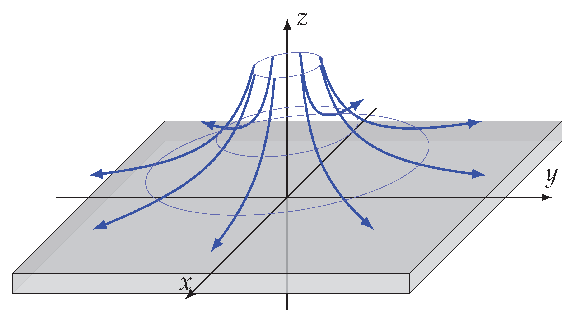
The problem of an axisymmetric stagnation flow against a solid wall, see Figure 1, is considered one of prototypical character in fluid mechanics, since the underlying features of Navier–Stokes theory are exposed, especially the formation of a boundary layer at the solid wall $z=0$. It is one of the few boundary layer problems that allow for an analytical treatment of the full NS equations, without the necessity of neglecting higher order terms. In the inviscid case, the velocity field, written in cylindrical coordinates ($r,\varphi ,z$), is given by Mayes et al. [61]:

$${\overrightarrow{u}}_{\mathrm{invis}}=Ar{\overrightarrow{e}}_r-2Az{\overrightarrow{e}}_z.$$

(69)

Although Equation (69) is a solution of the NS equations, it does not match to the no-slip condition ${\overrightarrow{e}}_r·\overrightarrow{u}=0$ at the wall and therefore represents a good approximation for the far field only, i.e., the field in the region $z\gg \sqrt{\nu /A}$ far beyond the boundary layer; whereas, in the vicinity of the wall, a boundary layer becomes manifest in which the velocity is assumed to take the slightly different form:

$$\overrightarrow{u}=r{f}^{\prime }\left(z\right){\overrightarrow{e}}_r-2f\left(z\right){\overrightarrow{e}}_z,$$

(70)

containing the function $f\left(z\right)$ that has to be determined. Note that the continuity Equation (53) is fulfilled identically by Equation (70). The associated boundary conditions are (i) the no-slip/no-penetration condition $\overrightarrow{u}=\overrightarrow{0}$ at $z=0$ and (ii) the matching condition $\overrightarrow{u}\to {\overrightarrow{u}}_{\mathrm{invis}}$ for $z\to \infty$, leading to:

$$f\left(0\right)=0,f^{\prime }\left(0\right)=0,\underset{z\to \infty }{lim}{f}^{\prime }\left(z\right)=A.$$

(71)

Now the extended Clebsch transformation developed in Section 2.3 is applied: writing the vorticity and the specific viscous force as:

$$\begin{array}{cc}\hfill \overrightarrow{\omega }& =\frac{r}{2}{f}^{\prime \prime }\left(z\right){\overrightarrow{e}}_{\varphi },\hfill \end{array}$$

(72)

$$\begin{array}{cc}\hfill 2\nu \nabla \times \overrightarrow{\omega }& =\nu \left[2f^{\prime \prime }\left(z\right){\overrightarrow{e}}_z-r{f}^{\prime \prime \prime }\left(z\right){\overrightarrow{e}}_r\right],\hfill \end{array}$$

(73)

the conditional equation simplifies to:

$$\frac{\partial \xi }{\partial \varphi }=0,$$

(74)

implying $\xi =\xi \left(r,z,t\right)$ as a general solution. Since a steady axisymmetric flow is considered, it is subsequently assumed independent of time and azimuthal angle for all potentials $\xi ,\alpha ,\beta$ and $\phi$. The remaining equations of interest are the generalised transport Equations (65) and (66) which, after minor mathematical manipulation, take the form:

$$\begin{array}{cc}\hfill \left[r^2{f}^{\prime }\left(z\right)f^{\prime \prime }\left(z\right)-2\nu f^{\prime \prime }\left(z\right)+\frac{\partial \xi }{\partial z}\right]\frac{\partial \alpha }{\partial r}-\left[2rf\left(z\right)f^{\prime \prime }\left(z\right)+\nu r{f}^{\prime \prime \prime }\left(z\right)+\frac{\partial \xi }{\partial r}\right]\frac{\partial \alpha }{\partial z}& =0,\hfill \end{array}$$

(75)

$$\begin{array}{cc}\hfill \left[r^2{f}^{\prime }\left(z\right)f^{\prime \prime }\left(z\right)-2\nu f^{\prime \prime }\left(z\right)+\frac{\partial \xi }{\partial z}\right]\frac{\partial \beta }{\partial r}-\left[2rf\left(z\right)f^{\prime \prime }\left(z\right)+\nu r{f}^{\prime \prime \prime }\left(z\right)+\frac{\partial \xi }{\partial r}\right]\frac{\partial \beta }{\partial z}& =0.\hfill \end{array}$$

(76)

The generalised Bernoulli Equation (64) and the continuity Equation (68) are decoupled from Equations (75) and (76); they provide the third Clebsch variable $\phi$ and the pressure p, both of which are not required here.

Three unknown fields $\xi ,\alpha ,\beta$ are involved in the two decisive PDEs (75) and (76) due to the freedoms given by the gauge symmetry with respect to the transformation in Equation (6). This provides the opportunity to choose the potentials in a beneficial way: for instance, by considering that the vorticity in Equation (72) can be written as $2\overrightarrow{\omega }=r{f}^{\prime \prime }\left(z\right){\overrightarrow{e}}_{\varphi }=r{f}^{\prime \prime }\left(z\right){\overrightarrow{e}}_z\times {\overrightarrow{e}}_r=\nabla f^{\prime }\left(z\right)\times \nabla r^2/2$ and comparison with Equation (14) motivates the choice:

$$\begin{array}{cc}\hfill \alpha & =f^{\prime }\left(z\right)\hfill \end{array}$$

(77)

$$\begin{array}{cc}\hfill \beta & =\frac{r^2}{2}\hfill \end{array}$$

(78)

for the two Clebsch variables. By inserting these into Equations (75) and (76), the following simplified equations:

$$\begin{array}{cc}\hfill \frac{\partial \xi }{\partial r}& =-2rf\left(z\right)f^{\prime \prime }\left(z\right)-\nu r{f}^{\prime \prime \prime }\left(z\right),\hfill \end{array}$$

(79)

$$\begin{array}{cc}\hfill \frac{\partial \xi }{\partial z}& =2\nu f^{\prime \prime }\left(z\right)-r^2{f}^{\prime }\left(z\right)f^{\prime \prime }\left(z\right),\hfill \end{array}$$

(80)

result for the auxiliary field which are both integrable, leading to:

$$\begin{array}{cc}\hfill \xi & =-r^{2}f\left(z\right)f^{\prime \prime }\left(z\right)-\frac{\nu }{2}{r}^2{f}^{\prime \prime \prime }\left(z\right)+F_1\left(z\right),\hfill \end{array}$$

(81)

$$\begin{array}{cc}\hfill \xi & =2\nu f^{\prime }\left(z\right)-\frac{r^2}{2}{f}^{\prime }{\left(z\right)}^2+F_2\left(r\right),\hfill \end{array}$$

(82)

containing the two integration functions $F_1\left(z\right)$ and $F_2\left(r\right)$. By subtracting Equation (81) from (82), the auxiliary field is eliminated, giving:

$$\frac{r^2}{2}\left[\nu f^{\prime \prime \prime }\left(z\right)+2f\left(z\right)f^{\prime \prime }\left(z\right)-f^{\prime }{\left(z\right)}^2\right]+F_2\left(r\right)+2\nu f^{\prime }\left(z\right)-F_1\left(z\right)=0.$$

(83)

Next, taking the limit $r\to 0$ of the above equation leads to $F_1\left(z\right)=F_2\left(0\right)+2\nu f^{\prime }\left(z\right)$; alternatively, the limit $z\to \infty$, in tandem with the matching condition $f^{\prime }\left(z\right)\to A$ according to Equation (71), gives $F_2\left(r\right)-F_2\left(0\right)=A^2{r}^2/2$. On re-inserting these explicit forms of the integration functions into Equation (83), the following ODE for the unknown function $f\left(z\right)$ is obtained:

$$\nu f^{\prime \prime \prime }\left(z\right)+2f\left(z\right)f^{\prime \prime }\left(z\right)-f^{\prime }{\left(z\right)}^2+A^2=0.$$

(84)

Finally, the substitution $f\left(z\right)=\sqrt{\nu A}\overline{f}\left(\overline{z}\right)$ with $\overline{z}=\sqrt{A/\nu }z$ transforms the latter into the more convenient form:

$${\overline{f}}^{\prime \prime \prime }\left(\overline{z}\right)+2\overline{f}\left(\overline{z}\right){\overline{f}}^{\prime \prime }\left(\overline{z}\right)-{\overline{f}}^{\prime }{\left(\overline{z}\right)}^2+1=0,$$

(85)

well-known in the literature as the Falkner-Skan equation [61].

3. Complex Variable and Tensor Potential Approach

3.1. The Classical Complex Variable Method

Consider the case of an arbitrary homogeneous continuum, with plane stress given by the tensor:

$$\underline{T}=\left(\begin{array}{cc}{\sigma }_x& {\tau }_{xy}\\ {\tau }_{xy}& {\sigma }_y\end{array}\right)$$

(86)

under a load provided by a conservative force with specific potential energy U. Assuming a steady state, the equilibrium condition:

$$\nabla ·\underline{T}+\varrho \nabla U=\overrightarrow{0}$$

(87)

has to be fulfilled. By defining the complex variable:

$$\xi :=x+\mathrm{i}y,$$

(88)

the three fields ${\sigma }_x,{\sigma }_y$ and ${\tau }_{xy}$ can be considered as functions of $\xi$ and its complex conjugate, $\overline{\xi }$, and the equilibrium Condition (87) reads:

$$\begin{array}{cc}\hfill \overrightarrow{0}& =\left(\frac{\partial }{\partial \xi }+\frac{\partial }{\partial \overline{\xi }},\mathrm{i}\frac{\partial }{\partial \xi }-\mathrm{i}\frac{\partial }{\partial \overline{\xi }}\right)\left(\begin{array}{cc}{\sigma }_x+\varrho U& {\tau }_{xy}\\ {\tau }_{xy}& {\sigma }_y+\varrho U\end{array}\right)\hfill \\ \hfill & =\frac{1}{2}\left(\begin{array}{c}\frac{\partial }{\partial \overline{\xi }}\left[{\sigma }_x+{\sigma }_y+2\varrho U\right]+\frac{\partial }{\partial \xi }\left[{\sigma }_x-{\sigma }_y+\mathrm{i}{\tau }_{xy}\right]+\mathrm{c}.\mathrm{c}.\\ -\mathrm{i}\frac{\partial }{\partial \overline{\xi }}\left[{\sigma }_x+{\sigma }_y+2\varrho U\right]-\mathrm{i}\frac{\partial }{\partial \xi }\left[{\sigma }_x-{\sigma }_y+\mathrm{i}{\tau }_{xy}\right]+\mathrm{c}.\mathrm{c}.\end{array}\right)\hfill \end{array}$$

(89)

where c.c. denotes the conjugate complex of the preceding expression. It is convenient to introduce the hydrostatic pressure $p:=({\sigma }_x+{\sigma }_y)/2$ and the complex stress $\underline{\sigma }:=({\sigma }_x-{\sigma }_y)/2+\mathrm{i}{\tau }_{xy}$, allowing Equation (89) to be written as $\Re \left(\partial \left[p+\varrho U\right]/\partial \overline{\xi }+\partial \underline{\sigma }/\partial \xi \right)=0$ and $\Im \left(\partial \left[p+\varrho U\right]/\partial \overline{\xi }+\partial \underline{\sigma }/\partial \xi \right)=0$ and therefore:

$$\frac{\partial }{\partial \overline{\xi }}\left[\frac{p}{\varrho }+U\right]+\frac{1}{\varrho }\frac{\partial \underline{\sigma }}{\partial \xi }=0,$$

(90)

as the complex form of the equilibrium Condition (87). The equilibrium Condition (90) is fulfilled identically by introducing a real-valued potential field $\Phi$ according to:

$$\begin{array}{cc}\hfill \frac{\underline{\sigma }}{\varrho }& =-4\frac{{\partial }^2\Phi }{\partial {\overline{\xi }}^2},\hfill \end{array}$$

(91)

$$\begin{array}{cc}\hfill \frac{p}{\varrho }+U& =4\frac{{\partial }^2\Phi }{\partial \overline{\xi }\partial \xi }.\hfill \end{array}$$

(92)

The potential $\Phi$ is the well known Airy stress function from the theory of linear elasticity [32,62]. Since, however, no assumptions regarding the constitutive equations of the respective continuum are required for the above derivation of the complex equilibrium Condition (87) and the use of Airy’s stress function according to Equations (91) and (92), this approach applies to any continuum and thus also to Stokes flow. By assuming a steady flow and neglecting the nonlinear terms for the case of very small Reynolds numbers, the NS Equations (52) simplify to the Stokes equation; being of the general form in Equation (87) with stress tensor $T_{ij}=-p{\delta }_{ij}+\varrho \nu \left({\partial }_i{u}_j+{\partial }_j{u}_i\right)$, leading to a complex stress field:

$$\frac{\underline{\sigma }}{\varrho }=-2\nu \frac{\partial u}{\partial \overline{\xi }},$$

(93)

where u denotes the complex velocity:

$$u=u_x+\mathrm{i}{u}_y.$$

(94)

On introducing a stream function $\mathsf{\Psi }$, satisfying:

$$u=-2\mathrm{i}\frac{\partial \mathsf{\Psi }}{\partial \overline{\xi }},$$

(95)

which fulfils the continuity Equation (53) identically [37,38], the constitutive Equation (93), written in terms of the stream function, becomes:

$$\frac{\underline{\sigma }}{\varrho }=4\mathrm{i}\nu \frac{{\partial }^2\mathsf{\Psi }}{\partial {\overline{\xi }}^2}.$$

(96)

By inserting Equation (96) into (91), the fully integrable equation:

$$\frac{{\partial }^2}{\partial {\overline{\xi }}^2}\left[\Phi +\mathrm{i}\nu \mathsf{\Psi }\right]=0,$$

(97)

results; the double integration of which gives the general solution:

$$\Phi +\mathrm{i}\nu \mathsf{\Psi }=g_0\left(\xi \right)+\overline{\xi }{g}_1\left(\xi \right),$$

(98)

containing integration functions $g_0\left(\xi \right)$ and $g_1\left(\xi \right)$, known as Goursat functions [62]. Note that, such an approach leads to the well-known Sherman–Lauricella equations [63,64,65] and to a reproduction of the Muskhelishvili–Kolosov formula [32,33].

The complex variable method has been applied successfully to various Stokes’ flow problems [35,66,67,68,69], usually by adopting a conformal mapping on the Goursat functions known for a simple flow domain in order to obtain the respective Goursat functions for a non-trivial domain. Being holomorphic, the Goursat functions can be recovered alternatively from their boundary values determined by the boundary conditions as utilised in [70,71,72] as an investigative tool for studying the internal flow structure of film flows over corrugated walls.

3.2. Integration of the Full 2D Navier–Stokes Equations

Making use again of the complex variable transformation in Equations (88) and (94), the NS Equations (52) and continuity Equation (53) can be reformulated as:

$$\begin{array}{cc}\hfill \frac{\partial u}{\partial t}+2\frac{\partial }{\partial \overline{\xi }}\left[\frac{\overline{u}u}{2}+\frac{p}{\varrho }+U\right]+2\frac{\partial }{\partial \xi }\left(\frac{u^2}{2}\right)& =4\nu \frac{{\partial }^{2}u}{\partial \overline{\xi }\partial \xi },\hfill \end{array}$$

(99)

$$\begin{array}{cc}\hfill \Re \left(\frac{\partial u}{\partial \xi }\right)& =0,\hfill \end{array}$$

(100)

in terms of the complex coordinate $\xi$, the complex velocity field u and their complex conjugates, with ℜ denoting the real part of the subsequent complex expression. It is obvious that by introducing a stream function $\mathsf{\Psi }$, according to Equation (95), the continuity Equation (100) is fulfilled identically. Accordingly, the complex NS Equation (99) can be written as:

$$\frac{\partial }{\partial \overline{\xi }}\left[\frac{\overline{u}u}{2}+\frac{p}{\varrho }+U-\mathrm{i}\frac{\partial \mathsf{\Psi }}{\partial t}\right]+\frac{\partial }{\partial \xi }\left(\frac{u^2}{2}\right)=2\nu \frac{{\partial }^{2}u}{\partial \overline{\xi }\partial \xi }.$$

(101)

By introducing a new complex potential M according to

$$\frac{\overline{u}u}{2}+\frac{p}{\varrho }+U-\mathrm{i}\frac{\partial \mathsf{\Psi }}{\partial t}=2\frac{\partial M}{\partial \xi },$$

(102)

an integrable form of Equation (99),

$$\frac{\partial }{\partial \xi }\left[2\frac{\partial M}{\partial \overline{\xi }}+\frac{u^2}{2}-2\nu \frac{\partial u}{\partial \overline{\xi }}\right]=0,$$

(103)

is obtained which, after integration with respect to $\xi$, gives:

$$2\frac{\partial M}{\partial \overline{\xi }}+\frac{u^2}{2}-2\nu \frac{\partial u}{\partial \overline{\xi }}=f\left(\overline{\xi }\right),$$

(104)

having integration function $f\left(\overline{\xi }\right)$ on the right hand side. The latter can be conveniently set to zero by re-gauging the potential M as follows:

$$M⟶M+\frac{1}{2}F\left(\overline{\xi }\right),$$

with $F^{\prime }\left(\overline{\xi }\right)=f\left(\overline{\xi }\right)$, since according to Equation (102) any complex function of $\overline{\xi }$ can be added to M without having any effect. Making use of Equation (95), Equation (104) simplifies to:

$$2\frac{\partial }{\partial \overline{\xi }}\left[M+2\mathrm{i}\nu \frac{\partial \mathsf{\Psi }}{\partial \overline{\xi }}\right]+\frac{u^2}{2}=0.$$

(105)

Finally, a second complex potential $\chi$ is introduced via:

$$M+2\mathrm{i}\nu \frac{\partial \mathsf{\Psi }}{\partial \overline{\xi }}=2\frac{\partial \chi }{\partial \overline{\xi }},$$

(106)

by which the two complex equations together with Equations (102) and (105) take the final form:

$$\begin{array}{cc}\hfill \frac{\overline{u}u}{2}+\frac{p}{\varrho }+U-\mathrm{i}\left[\frac{\partial \mathsf{\Psi }}{\partial t}-4\nu \frac{{\partial }^2\mathsf{\Psi }}{\partial \overline{\xi }\partial \xi }\right]& =4\frac{{\partial }^2\chi }{\partial \overline{\xi }\partial \xi },\hfill \end{array}$$

(107)

$$\begin{array}{cc}\hfill -\frac{u^2}{2}& =4\frac{{\partial }^2\chi }{\partial {\overline{\xi }}^2}.\hfill \end{array}$$

(108)

By Equations (107) and (108), two complex equations are given containing the complex potential $\chi$, the real-valued stream function $\mathsf{\Psi }$ and the pressure p as unknowns. They constitute a first integral of Navier–Stokes equations [73] in the sense that by taking the difference of the derivative of Equation (108) with respect to $\xi$ with the derivative of Equation (107) with respect to $\overline{\xi }$, the complex NS Equation (99) is recovered.

Compared to the classical complex variable approach outlined in Section 3.1, a complex valued potential field $\chi$ is required for the integration of the full 2D-NS equation in place of the real valued Airy stress function $\Phi$ utilised for the Stokes equation. A relationship between $\chi$ and $\Phi$ can be established for the particular case of steady flow: by setting $\partial \mathsf{\Psi }/\partial t=0$, Equation (107) simplifies to:

$$\frac{\overline{u}u}{2}+\frac{p}{\varrho }+U=4\frac{{\partial }^2}{\partial \overline{\xi }\partial \xi }\left[\chi -\mathrm{i}\nu \mathsf{\Psi }\right],$$

which, apart from the additional nonlinear term $\overline{u}u/2$, corresponds to Equation (92) if $\Phi =\chi -\mathrm{i}\nu \mathsf{\Psi }$ is identified as the Airy stress function. Thus, for the steady flow case the two field Equations (107) and (108) simplify to:

$$\begin{array}{cc}\hfill \frac{\overline{u}u}{2}+\frac{p}{\varrho }+U& =4\frac{{\partial }^2\Phi }{\partial \overline{\xi }\partial \xi },\hfill \end{array}$$

(109)

$$\begin{array}{cc}\hfill 4\mathrm{i}\nu \frac{{\partial }^2\mathsf{\Psi }}{\partial {\overline{\xi }}^2}+\frac{u^2}{2}& =-4\frac{{\partial }^2\Phi }{\partial {\overline{\xi }}^2},\hfill \end{array}$$

(110)

in accordance with [38]. Note that Equation (109) takes the form of Bernoulli’s equation apart from the second order derivative of the potential on its right hand side.

3.3. Integration of the Dynamic Boundary Condition

The mathematical derivation is completed by the specification of appropriate boundary conditions, which take the form of no-slip/no-penetration conditions at solid walls, inflow and outflow conditions and, in the case of film or multiphase flows, kinematic and dynamic boundary conditions at a free surface or internal interface. These are discussed in detail in [38,73]. However, a key feature of the above approach that requires emphasising is that the dynamic boundary condition associated with a free surface or internal interface can be similarly integrated in the case of steady flow leading to a corresponding first integral form that greatly simplifies enforcing such a condition compared to the standard method of addressing such problems employing the standard NS equations and boundary conditions written in primitive (i.e., observable) variables. Accordingly, this case as outlined briefly below.

Consider a simply connected domain with a boundary $\xi =f\left(s\right)$, parametrised with respect to the arc length s of the boundary; furthermore, tangential and normal unit vectors along the boundary are taken to be $f^{\prime }\left(s\right)$ and $n=\mathrm{i}{f}^{\prime }\left(s\right)$, respectively. In terms of the stream function $\mathsf{\Psi }$, the kinematic boundary condition $\Im (u{\overline{f}}^{\prime })=0$ ensures that along a free surface/interface the velocity in the normal direction vanishes, resulting in:

$$\frac{\partial \mathsf{\Psi }}{\partial s}=0.$$

(111)

The original dynamic boundary condition, after transformation into complex representation, reads:

$$\frac{p_0-p}{\varrho }n-2\mathrm{i}\nu \frac{\partial u}{\partial \overline{\xi }}{\overline{f}}^{\prime }=\frac{\sigma }{\varrho }{f}^{\prime \prime }.$$

(112)

By making use of Equations (109) and (110), the pressure p and the viscous stresses $\mathrm{i}\nu \partial u/\partial \overline{\xi }$ can be replaced by derivatives of $\Phi$, implying:

$$-u\frac{\mathrm{d}\mathsf{\Psi }}{\mathrm{d}s}+\left(U+\frac{p_0}{\varrho }\right)n=\frac{\mathrm{d}}{\mathrm{d}s}\left[\frac{\sigma }{\varrho }{f}^{\prime }+4\mathrm{i}\frac{\partial \Phi }{\partial \overline{\xi }}\right],$$

(113)

as the boundary condition for $\Phi$. Since the specific potential energy U can be gauged with a constant, $U+p_0/\varrho$ can be replaced by U. Making use of the kinematic boundary condition in Equation (111), integration of Equation (113) leads to:

$$4\mathrm{i}\frac{\partial \Phi }{\partial \overline{\xi }}=-\frac{\sigma }{\varrho }{f}^{\prime }+\int Un\mathrm{d}s,$$

(114)

as a first integral of the dynamic boundary condition. In [38], the same boundary condition is derived in real-valued form and where it is demonstrated that it can be decomposed into a Dirichlet and a Neumann boundary condition for $\Phi$. The reduction of the original non-standard boundary condition in Equation (112) containing mixed contributions from different fields u and p to a mathematical standard form has proven to be extremely beneficial for the implementation of numerical methods of solution, as demonstrated in [6,38,74].

3.4. Particular Flow Geometries as Exemplars

Three different flow problems are used to demonstrate applications of the tensor approach described above; two of which lead to closed form analytical solutions, the third requiring a numerical solution.

3.4.1. Uniaxial Flow: Flow over an Oscillating Plate

Consider the case of a uniaxial flow geometry with, $u_y=0$, or equivalently in complex formulation: $u-\overline{u}=0$. With reference to Equation (95), the following PDE:

$$\frac{\partial \mathsf{\Psi }}{\partial \xi }+\frac{\partial \mathsf{\Psi }}{\partial \overline{\xi }}=0$$

has to be satisfied, implying the following explicit forms:

$$\begin{array}{ccc}\hfill \mathsf{\Psi }& =& \mathsf{\Psi }\left(\frac{\xi +\overline{\xi }}{2\mathrm{i}},t\right)=\mathsf{\Psi }\left(y,t\right)\hfill \end{array}$$

(115)

$$\begin{array}{ccc}\hfill u& =& -2\mathrm{i}\frac{\partial \mathsf{\Psi }}{\partial \overline{\xi }}={\mathsf{\Psi }}^{\prime }\left(y,t\right)\hfill \end{array}$$

(116)

for the stream function and the velocity; the prime denotes differentiation with respect to y. The general solution of Equation (108) is given by:

$$\chi =\overline{\xi }{w}_0(\xi ,t)+w_1(\xi ,t)+\frac{1}{2}\int \left[\int {\mathsf{\Psi }}^{\prime }{\left(y,t\right)}^2\mathrm{d}y\right]\mathrm{d}y,$$

(117)

containing the two analytic functions $w_0(\xi ,t)$, $w_1(\xi ,t)$, being generalisations of the so-called Goursat functions [38]. Following the insertion of Equation (117), Equation (107) simplifies to:

$$\frac{p}{\varrho }+U-\mathrm{i}\left[\dot{\mathsf{\Psi }}-\nu {\mathsf{\Psi }}^{\prime \prime }\right]=4w_0^{\prime }(\xi ,t):,$$

(118)

the dot over a symbol denoting its time-derivative.

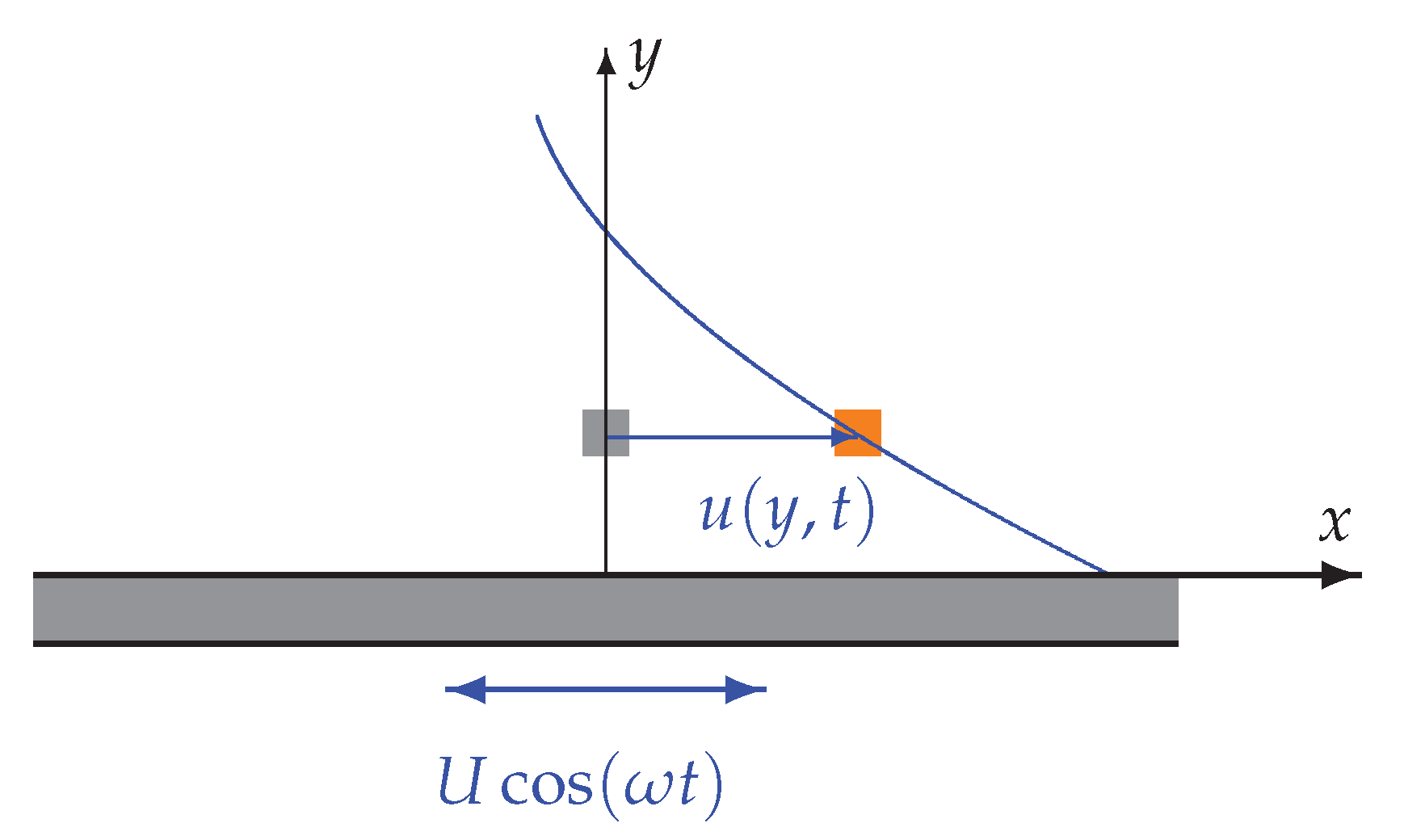
A horizontal plate of infinite extent covered by a fluid invokes a flow by a forced oscillatory movement, see Figure 2.

The no-penetration condition is already fulfilled due to the prescribed flow configuration $u_y=0$, while the no-slip condition compels the fluid to mimic the oscillatory behaviour of the plate according to $u_x(y,0)=Ucos\left(\omega t\right)$. By re-writing the latter in terms of the stream function $\mathsf{\Psi }$ via $u_x=\partial \mathsf{\Psi }/\partial y$, it takes the form of a Neumann boundary condition ${\mathsf{\Psi }}^{\prime }(0,t)=Ucos\left(\omega t\right)$. Since the stream function is gaugeable by an arbitrary constant, the additional Dirichlet condition $\mathsf{\Psi }(0,t)=0$ can be formulated without loss of generality. Additionally, the asymptotic condition ${\mathsf{\Psi }}^{\prime }(y,t)\to 0$ has to be fulfilled to ensure that the fluid tends to a state at rest far away from the plate.

Assuming vanishing pressure $p=0$ and a wave-like solution of the form

$$\mathsf{\Psi }=U\Im \left\{exp(-\mathrm{i}\omega t)\frac{exp\left(\mathrm{i}ky\right)-1}{k}\right\},$$

(119)

together with fulfilment of the no-slip and no-penetration condition, then Equation (118) leads to the identity:

$$-\mathrm{i}U\Im \left\{\frac{-\mathrm{i}\omega +\nu k^2}{k}exp\left(\mathrm{i}[ky-\omega t]\right)+\mathrm{i}\frac{\omega }{k}exp(-\mathrm{i}\omega t)\right\}=4w_0^{\prime }(\xi ,t),$$

requiring k and $\omega$ to satisfy the dispersion relation:

$$\mathrm{i}\omega =\nu k^2$$

(120)

for damped transverse waves in accordance to the classical result [22]. The Goursat function $w_0$ takes the form:

$$w_0=-\frac{\mathrm{i}}{4}\xi \nu U\Im \left[kexp(-\mathrm{i}\omega t)\right].$$

(121)

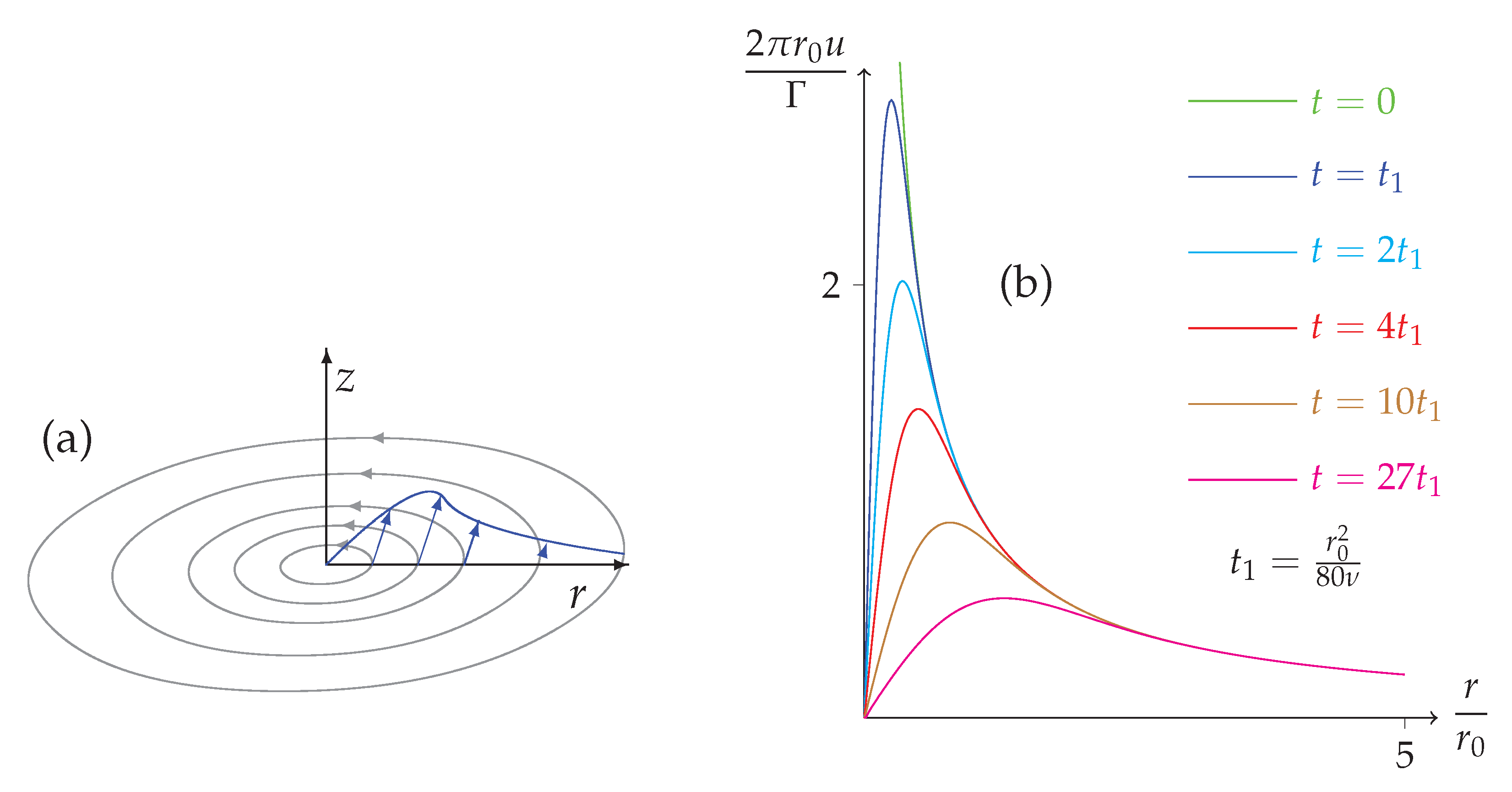
3.4.2. Axisymmetric Flow: The Lamb-Oseen Vortex

Consider a class of flows given by the following particular form:

$$\begin{array}{ccc}\hfill \mathsf{\Psi }& =& \mathsf{\Psi }(r,t),\hfill \end{array}$$

(122)

$$\begin{array}{ccc}\hfill u& =& -2\mathrm{i}\frac{\partial \mathsf{\Psi }}{\partial \overline{\xi }}=-\frac{\mathrm{i}\xi }{r}{\mathsf{\Psi }}^{\prime }\left(r,t\right),\hfill \end{array}$$

(123)

$$\begin{array}{ccc}\hfill r& :=& \sqrt{\overline{\xi }\xi },\hfill \end{array}$$

(124)

of the stream function with the prime denoting differentiation with respect to r; that is flows, the streamlines of which form concentric circles, see Figure 3a. Assuming a particular solution for Equation (108) of the form ${\chi }_{\mathrm{p}}={\chi }_{\mathrm{p}}(r,t)$ leads to the the following expression:

$$r\frac{\partial }{\partial r}\left(\frac{{\chi }_{\mathrm{p}}^{\prime }}{r}\right)=\frac{1}{2}{\mathsf{\Psi }}^{\prime }{\left(r,t\right)}^2,$$

(125)

and therefore:

$$\frac{{\chi }_{\mathrm{p}}^{\prime }}{r}=\frac{1}{2}\int \frac{{\mathsf{\Psi }}^{\prime }{\left(r,t\right)}^2}{r}\mathrm{d}r.$$

(126)

By inserting the above into Equation (107), the following simplified PDE results:

$$\frac{p}{\varrho }+U-\mathrm{i}\left[\dot{\mathsf{\Psi }}-\frac{\nu }{r}\frac{\partial }{\partial r}\left(r{\mathsf{\Psi }}^{\prime }\right)\right]-\int \frac{{\mathsf{\Psi }}^{\prime }{\left(r,t\right)}^2}{r}\mathrm{d}r=0.$$

(127)

Via the introduction of the following similarity variable:

$$z=\frac{r}{\sqrt{\nu t}}$$

solutions of the form $\mathsf{\Psi }=f\left(z\right)$ are now searched for. Under the above assumptions the imaginary part of Equation (127) takes the form:

$$\frac{1}{t}\left[\frac{z}{2}{f}^{\prime }\left(z\right)+\frac{1}{z}\frac{\mathrm{d}}{\mathrm{d}z}\left(z{f}^{\prime }\left(z\right)\right)\right]=0$$

which, after making the substitution $g\left(z\right)=z{f}^{\prime }\left(z\right)$, can be written conveniently as;

$$g^{\prime }\left(z\right)+\frac{z}{2}g\left(z\right)=0,$$

which, in turn, is easily solved by taking:

$$g\left(z\right)=g_{0}exp\left(-\frac{z^2}{4}\right),$$

(128)

leading to:

$$f\left(z\right)=g_0\int \frac{1}{z}exp\left(-\frac{z^2}{4}\right)\mathrm{d}z=\frac{g_0}{2}\mathrm{Ei}\left(-\frac{z^2}{4}\right),$$

(129)

where Ei denotes the integral exponential function. This particular solution contains a singularity; however, by considering the superposition:

$$\mathsf{\Psi }=\frac{g_0}{2}\mathrm{Ei}\left(-\frac{z^2}{4}\right)-\frac{\Gamma }{2\pi }lnr,$$

with the well-known potential vortex $\frac{\Gamma }{2\pi }lnr$ as an alternative solution to Equation (127), the singularity is removed as follows: the complex velocity field resulting from Equation (123) reads

$$u=-\frac{\mathrm{i}\xi }{r}{\mathsf{\Psi }}^{\prime }\left(r,t\right)=\frac{\mathrm{i}}{r}\left[\frac{\Gamma }{2\pi }+g_{0}exp\left(-\frac{r^2}{4\nu t}\right)\right]exp\left(\mathrm{i}\phi \right),$$

which is convergent in the limit $r\to 0$ if and only if $2\pi g_0=\Gamma$. Finally, the solution reads:

$$u=\frac{\mathrm{i}\Gamma }{2\pi r}\left[1-exp\left(-\frac{r^2}{4\nu t}\right)\right]exp\left(\mathrm{i}\phi \right),$$

(130)

which is a reproduction of the classical Lamb-Oseen vortex [19]. The velocity profile $\left|u\right|$ is shown in Figure 3b.

3.4.3. Steady Film Flow over Topography

In the context of the numerical solution of flow problems, possibly involving a free surface, for which inertial effects cannot be ignored, the LSFEM, Cassidy [75], Thatcher [76], Bolton and Thatcher [77], has gained wide acceptability as a very effective and flexible approach—in particular when simple equal order elements in conjunction with highly efficient multigrid solvers are employed [6], exploiting the symmetry and positive definiteness of the resulting system matrices [78].

For reasons of practicality, the complex field Equations (109) and (110) are expressed as real-valued ones in terms of the velocity variables $u_x=\Re u={\partial }_y\mathsf{\Psi }$, $u_y=\Im u=-{\partial }_x\mathsf{\Psi }$ and first order derivatives, ${\varphi }_x={\partial }_x\Phi$, ${\varphi }_y={\partial }_y\Phi$, of the Airy stress function leading, together with the continuity Equation (53) and the condition:

$$\frac{\partial {\varphi }_1}{\partial y}-\frac{\partial {\varphi }_2}{\partial x}=0,$$

(131)

to a system of four equations involving first order derivatives of $u_x,u_y,{\varphi }_x,{\varphi }_y$ only, conforming ideally to a first-order system least squares methodology.

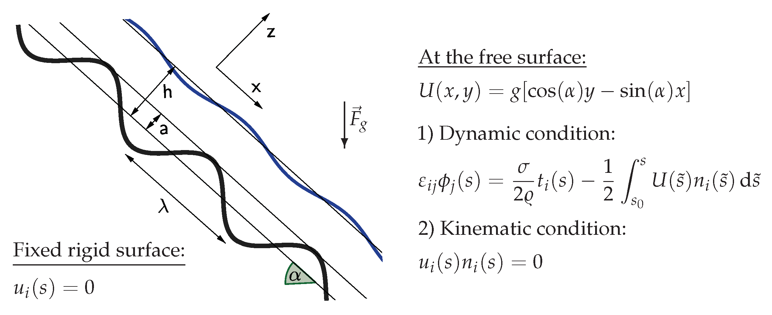
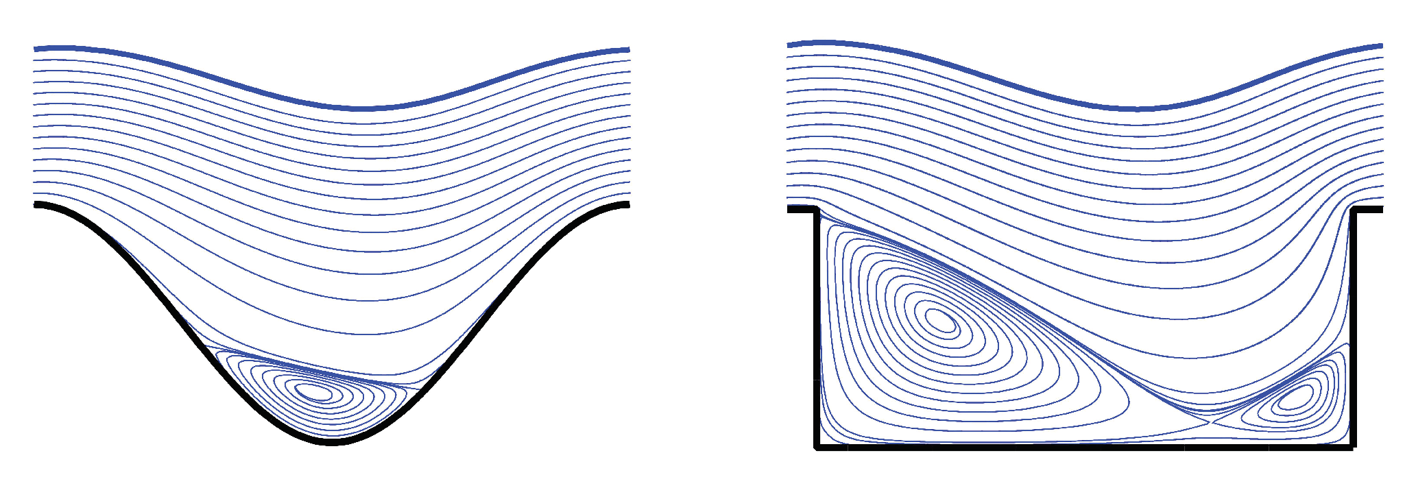
Figure 4 shows the problem of gravity-driven film flow down a corrugated rigid surface inclined at an angle $\alpha$ to the horizontal considered by Marner [6]. Along the stationary corrugated surface, velocity Dirichlet conditions are imposed. While at the free surface, in addition to a kinematic boundary condition, two dynamic conditions are imposed resulting as inhomogeneous Dirichlet conditions for ${\varphi }_1$ and ${\varphi }_2$ from Equation (114) by decomposition into real and imaginary parts; these depend on the surface tension, the curvature and the potential energy density. The resulting free surface profile is obtained by iterating over the kinematic condition while solving a sequence of flow problems with prescribed dynamic conditions in a fixed domain using the LSFEM.

Two representative results for two differently contoured and repeating surface shapes are shown in Figure 5:

The resulting streamline patterns reproduce exactly the observed corresponding experimental results of [79], obtained using silicon oil Elbesil 145: $\varrho =964.8\mathrm{kg}/{\mathrm{m}}^3$, $\nu =144.2{\mathrm{mm}}^2/\mathrm{s}$, $\sigma =20.1\mathrm{mN}/\mathrm{m}$, $\lambda =20\mathrm{mm}$, $A=4\mathrm{mm}$, $H_0=5\mathrm{mm}$, $\alpha ={10}^{\circ }$.

Overall, the numerical method was shown [6] to produce an accurate and reliable result over a wide range of Reynolds and capillary numbers for the above problem.

3.5. Tensor Potential Approach

The obvious limitation of the 2D complex-variable formulation is its extension beyond two dimensions, since for the case of 3D viscous flow, a corresponding complex first integral formulation is, by definition, not possible; however, a real-valued tensor form is. In two dimensions, such a form can be established by decomposing both Equations (108) and (107) into real and imaginary parts and taking the linear combinations ℜ(107)$\pm \Re$(108), leading to four real-valued equations:

$$\begin{array}{cc}\hfill u_1^2+\frac{p}{\varrho }+U=& 2{\partial }_2^2\Re \chi +2{\partial }_1{\partial }_2\Im \chi ,\hfill \end{array}$$

(132)

$$\begin{array}{cc}\hfill u_2^2+\frac{p}{\varrho }+U=& 2{\partial }_1^2\Re \chi -2{\partial }_1{\partial }_2\Im \chi ,\hfill \end{array}$$

(133)

$$\begin{array}{cc}\hfill u_1{u}_2=& -\left\{{\partial }_1^2-{\partial }_2^2\right\}\Im \chi -2{\partial }_1{\partial }_2\Re \chi ,\hfill \end{array}$$

(134)

$$\begin{array}{cc}\hfill {\partial }_t\mathsf{\Psi }=& -{\nabla }^2\left[\Im \chi -\nu \mathsf{\Psi }\right],\hfill \end{array}$$

(135)

which, in the context of extension to higher dimensions, can be written in the following convenient and compact tensor form:

$$u_i{u}_j+\left[\frac{p}{\varrho }+U\right]{\delta }_{ij}=-{\partial }_k{\partial }_k{\tilde{a}}_{ij}+{\partial }_i{A}_j+{\partial }_j{A}_i-{\partial }_k{A}_k{\delta }_{ij},$$

(136)

with the tensor and vector fields given by ${\tilde{a}}_{ij}=-\Re \chi {\delta }_{ij}$ and $A_j={\partial }_i{\tilde{a}}_{ij}+{\epsilon }_{jk}{\partial }_k\Im \chi$, respectively. The abbreviations ${\partial }_k:=\partial /\partial x_k$ and ${\partial }_t:=\partial /\partial t$ imply partial differentiation, while ${\delta }_{ij}$ and ${\epsilon }_{ij}$ denote the Kronecker delta function and the two-dimensional Levi-Civita symbol, respectively.

Recently [39], the corresponding tensor potential formulation for three dimensions has been established, an essential underpinning being analogies drawn with the methodical reduction of Maxwell’s equations [6]. The continuity Equation (53) is shown to be fulfilled identically following the introduction a streamfunction vector ${\mathsf{\Psi }}_k$ for the velocity, in accordance with $u_i={\epsilon }_{ijk}{\partial }_j{\mathsf{\Psi }}_k$ and ${\epsilon }_{ijk}$ denoting the corresponding 3D Levi-Civita symbol, representing a 3D generalisation of the 2D streamfunction [21]. Compared to the 2D first integral of the NS equations, the corresponding 3D formulation utilises an independent symmetric tensor potential ${\tilde{a}}_{ij}$ and a vector potential ${\phi }_i$ with the indices $i,j$ taking values from 1 to 3. The auxiliary vector field $A_j$ in the 3D case reads:

$$A_j={\partial }_k{\tilde{a}}_{kj}+{\epsilon }_{jlk}{\partial }_l{\phi }_k,$$

(137)

and Equation (135) has to replaced by its corresponding 3D form:

$$\begin{array}{c}\hfill {\partial }_t{\mathsf{\Psi }}_n=\nu {\partial }_k{\partial }_k{\mathsf{\Psi }}_n-{\epsilon }_{nkl}{\partial }_k{\partial }_m{\tilde{a}}_{ml}.\end{array}$$

(138)

Like the Clebsch variables considered in Section 2, the tensor potential ${\tilde{a}}_{ij}$ and the vector potential ${\phi }_i$ are not unique and can be gauged in a beneficial way. Obviously, by performing the operations:

$$\begin{array}{cc}\hfill {\tilde{a}}_{ij}& ⟶{\tilde{a}}_{ij}+{\partial }_i{\alpha }_j+{\partial }_j{\alpha }_i-{\partial }_k{\alpha }_k{\delta }_{ij},\hfill \end{array}$$

(139)

$$\begin{array}{cc}\hfill {\phi }_i& ⟶{\phi }_i+{\partial }_i\zeta ,\hfill \end{array}$$

(140)

for an arbitrary vector field ${\alpha }_i$ and an arbitrary scalar field $\zeta$, the field Equations (136) remain invariant. These rules are utilised in [39] to establish bona fide gauging scenarios. In the same paper the prescription of appropriate commonly occurring physical and necessary auxiliary boundary conditions, incorporating for completeness the derivation of a first integral of the dynamic boundary condition at a free surface, is established, together with how the general approach can be advantageously reformulated for application in solving unsteady flow problems with periodic boundaries.

Using a tensor formulation, the approach is suitable for use in the case of an arbitrary number of dimensions: in [80], a potential-based first integral form is established for the 4D energy-momentum equations for flows under relativistic conditions.

4. Discussion

Based on a detailed analysis and discourse, the two different approaches considered above can be explained in the light of their different origins: the Clebsch representation of the velocity can, according to recent analysis [56], be understood as a natural outcome of Galilean invariance; whereas, Airy’s stress function originates historically from the 2D static equilibrium of internal forces. In the course of a long and growing series of research contributions both approaches have been generalised and made available for use in solving arbitrary flow problems. A Clebsch transformation has emerged that applies to arbitrary forces in the equations of motion, including viscous ones, while extensions to the Airy stress function approach applies to cases beyond static equilibrium, in particular to unsteady flows with inertia and, after rearrangement of the complex equations, to tensor equations (in terms of a tensor potential) for 3D viscous flows and even for the case of 4D relativistic flows. The use of a tensor potential has parallels to Maxwell’s theory of electromagnetism [6,39,80]. The capabilities of both approaches have been convincingly demonstrated through the solution of a variety of illustrative examples.

Despite the very positive stage of development of both methods, some open questions remain: the first is that the field Equations (64)–(68) resulting, via the extended Clebsch transformation according to Theorem 2, from the NS equations are not self-adjoint; as in the inviscid flow case. The non-existence of a Lagrangian appears to be due to energy dissipation caused by viscosity. Anthony [81] poses a possible strategy to overcome this problem by including thermal degrees of freedom and related inner energy in order to remain consistent with Noether’s theorem, which implies conservation of energy for Lagrangians being invariant with respect to time-translations. Note that the present work, by dissipation, the irreversible transfer of energy from mechanical to thermal energy is understood from the physicist’s viewpoint, while the total energy (the sum of mechanical and thermal energy) is conserved. Based on Seliger and Witham [24]’s classical work, Zuckerwar and Ash [82], Zuckerwar and Ash [83] suggest a Lagrangian considering only volume viscosity, leading to equations of motion containing, only qualitatively, the effect of volume viscosity but differing quantitatively from the compressible NS equations—also known as the Navier–Stokes–Duhem equations [84,85] without shear viscosity. They interpret their result as a generalisation of the theory of viscous flow towards thermodynamic non-equilibrium. A Lagrangian for viscous flow considering both shear viscosity and volume viscosity has been suggested by Scholle and Marner [86], Marner et al. [87], again leading to equations of motion that differ from the Navier–Stokes–Duhem equations by non-equilibrium terms. A striking feature of their Lagrangian is a discontinuity, causing fluctuations on a microscopic scale and revealing parallels to a stochastic variational description as in statistical physics; see, for example, [88,89,90,91,92,93]. Since these considerations go beyond the scope of classical fluid mechanics, further research on this particular field is required.

A second unanswered question is whether a general and all-encompassing potential approach exists reducing to both the Clebsch and the tensor potential approach as special cases. The search for this ’missing link’ between two conceptually different approaches represents another future research topic of general interest. A promising first step could be an analysis of the Clebsch transformation in the sense of general relativity [94], followed by a particular classical limit as shown in Lightman et al. [95], problem 5.31 pp. 35, 227–228.

Thirdly, the first integral of the 4D energy-momentum equations based on a tensor potential [80] points to the future use of mathematical techniques and methods of solutions not currently applicable to the field equations in their original form, in particular the use of matrix structures within the framework of Clifford algebra, based on quaternions or Dirac matrices with the goal of developing highly efficient methods of solution. Having mapped the entire problem to a matrix-algebra framework, the limit $c\to \infty$ could be applied in order to provide efficient solutions of the classical NS equations. Although implementation of such a matrix-algebra techniques remains speculative at this stage, it deserves further investigation since its utilisation can lead to significant economic gains in the computation of fluid flows, in a similar fashion to the use of quaternions representing spatial rotation operations [96,97], potentially leading to the formulation of highly efficient and predictive CFD software.

References

- Jackson, J.D. Classical Electrodynamics, 3rd ed.; Wiley: New York, NY, USA, 1999. [Google Scholar]
- Heaviside, O. Electrical Papers (2 Volumes, Collected Works); The Electrician Printing and Publishing Co.: London, UK, 1892. [Google Scholar]
- Heaviside, O. Electromagnetic Theory; The Electrician Printing and Publishing Co.: London, UK, 1894; Volume 1. [Google Scholar]
- Wu, A.; Yang, C.N. Evolution of the concept of the vector potential in the description of fundamental interactions. Int. J. Mod. Phys. A 2006, 21, 3235–3277. [Google Scholar] [CrossRef]
- Jackson, J.D.; Okun, L.B. Historical roots of gauge invariance. Rev. Mod. Phys. 2001, 73, 663–680. [Google Scholar] [CrossRef] [Green Version]
- Marner, F. Potential-Based Formulations of the Navier-Stokes Equations and Their Application. Ph.D. Thesis, Durham University, Durham, UK, 2019. [Google Scholar]
- Kaku, M. Quantum Field Theory: A Modern Introduction; Oxford University Press: Oxford, UK, 1993. [Google Scholar]
- Lanczos, C. The Splitting of the Riemann Tensor. Rev. Mod. Phys. 1962, 34, 379–389. [Google Scholar] [CrossRef]
- Roberts, M.D. The Lanczos Potential for Bianchi Spacetime. arXiv 2019, arXiv:1910.00416. [Google Scholar]
- Ehrenberg, W.; Siday, R.E. The Refractive Index in Electron Optics and the Principles of Dynamics. Proc. Phys. Soc. B 1949, 62, 8–21. [Google Scholar] [CrossRef]
- Aharonov, Y.; Bohm, D. Significance of Electromagnetic Potentials in the Quantum Theory. Phys. Rev. 1959, 115, 485–491. [Google Scholar] [CrossRef]
- Boyer, T.H. Does the Aharonov–Bohm Effect Exist? Found. Phys. 2000, 30, 893–905. [Google Scholar] [CrossRef]
- Boyer, T.H. Comment on Experiments Related to the Aharonov–Bohm Phase Shift. Found. Phys. 2008, 38, 498–505. [Google Scholar] [CrossRef] [Green Version]
- Vaidman, L. Role of potentials in the Aharonov-Bohm effect. Phys. Rev. A 2012, 86, 040101. [Google Scholar] [CrossRef] [Green Version]
- Aharonov, Y.; Cohen, E.; Rohrlich, D. Comment on “Role of potentials in the Aharonov-Bohm effect”. Phys. Rev. A 2015, 92. [Google Scholar] [CrossRef] [Green Version]
- Vaidman, L. Reply to “Comment on ‘Role of potentials in the Aharonov-Bohm effect”’. Phys. Rev. A 2015, 92, 026102. [Google Scholar] [CrossRef] [Green Version]
- Aharonov, Y.; Cohen, E.; Rohrlich, D. Nonlocality of the Aharonov-Bohm effect. Phys. Rev. A 2016, 93, 042110. [Google Scholar] [CrossRef] [Green Version]
- De Oliveira, C.R.; Romano, R.G. A New Version of the Aharonov-Bohm Effect. Found. Phys. 2020, 50, 137–146. [Google Scholar] [CrossRef] [Green Version]
- Lamb, H. Hydrodynamics; Cambridge University Press: Cambridge, UK, 1974. [Google Scholar]
- Panton, R.L. Incompressible Flow; John Wiley & Sons, Inc.: Hoboken, NJ, USA, 1996. [Google Scholar]
- Batchelor, G.K. An Introduction to Fluid Dynamics; Cambridge Mathematical Library, Cambridge University Press: Cambridge, UK, 2000. [Google Scholar]
- Spurk, J.H.; Aksel, N. Fluid Mechanics, 2nd ed.; Springer: Berlin/Heidelberg, Germany, 2008. [Google Scholar] [CrossRef]
- Clebsch, A. Ueber die Integration der hydrodynamischen Gleichungen. Journal für die Reine und Angewandte Mathematik 1859, 56, 1–10. [Google Scholar]
- Seliger, R.; Witham, G.B. Variational principles in continuum mechanics. Proc. R. Soc. Lond. A Math. Phys. Eng. Sci. 1968, 305, 1–25. [Google Scholar] [CrossRef]
- Wagner, H.J. Das Inverse Problem der Lagrangeschen Feldtheorie in Hydrodynamik, Plasmaphysik und Hydrodynamischem Bild der Quantenmechanik. Ph.D. Thesis, University of Paderborn, Paderborn, Germany, 1997. [Google Scholar]
- Calkin, M.G. An action principle for magnetohydrodynamics. Can. J. Phys. 1963, 41, 2241–2251. [Google Scholar] [CrossRef]
- Rund, H. Clebsch representations and relativistic dynamical systems. Arch. Ration. Mech. Anal. 1979, 71, 199–220. [Google Scholar] [CrossRef]
- Madelung, E. Quantentheorie in hydrodynamischer Form. Zeitschrift für Physik 1927, 40, 322–326. [Google Scholar] [CrossRef]
- Schoenberg, M. Vortex Motions of the Madelung Fluid. Nuovo Cimento 1955, 1, 543–580. [Google Scholar] [CrossRef]
- Roberts, M. A fluid generalization of membranes. Open Phys. 2011, 9, 1016–1021. [Google Scholar] [CrossRef] [Green Version]
- Asenjo, F.A.; Mahajan, S.M. Relativistic quantum vorticity of the quadratic form of the Dirac equation. Phys. Scr. 2015, 90, 015001. [Google Scholar] [CrossRef]
- Muskhelishvili, N.I. Some Basic Problems of the Mathematical Theory of Elasticity; Noordhoff: Groningen, The Netherlands, 1953. [Google Scholar]
- Mikhlin, S.G. Integral Equations and Their Applications to Certain Problems in Mechanics, Mathematical Physics and Technology; Pergamon Press: New York, NY, USA, 1957. [Google Scholar]
- Legendre, R. Solutions plus complète du problème Blasius. Comptes Rendus Hebdomadaires des Seances de l Academie des Sciences 1949, 228, 2008–2010. [Google Scholar]
- Coleman, C.J. On the use of complex variables in the analysis of flows of an elastic fluid. J. Non-Newtonian Fluid Mech. 1984, 15, 227–238. [Google Scholar] [CrossRef]
- Ranger, K.B. Parametrization of general solutions for the Navier-Stokes equations. Q. J. Appl. Math. 1994, 52, 335–341. [Google Scholar] [CrossRef] [Green Version]
- Scholle, M.; Haas, A.; Gaskell, P.H. A first integral of Navier-Stokes equations and its applications. Proc. R. Soc. A 2011, 467, 127–143. [Google Scholar] [CrossRef] [Green Version]
- Marner, F.; Gaskell, P.H.; Scholle, M. On a potential-velocity formulation of Navier-Stokes equations. Phys. Mesomech. 2014, 17, 341–348. [Google Scholar] [CrossRef]
- Scholle, M.; Gaskell, P.H.; Marner, F. Exact integration of the unsteady incompressible Navier-Stokes equations, gauge criteria, and applications. J. Math. Phys. 2018, 59, 043101. [Google Scholar] [CrossRef] [Green Version]
- Neuber, H. Ein neuer Ansatz zur Lösung räumlicher Probleme der Elastizitätstheorie. J. Appl. Math. Mech. 1934, 14, 2008–2010. [Google Scholar]
- Lee, S.; Ryi, S.; Lim, H. About vortex equations of two dimensional flows. Indian J. Phys. 2017, 91, 1089–1094. [Google Scholar] [CrossRef]
- Greengard, L.; Jiang, S. A New Mixed Potential Representation for Unsteady, Incompressible Flow. SIAM Rev. 2019, 61, 733–755. [Google Scholar] [CrossRef]
- Prakash, J.; Lavrenteva, O.M.; Nir, A. Application of Clebsch variables to fluid-body interaction in presence of non-uniform vorticity. Phys. Fluids 2014, 26, 077102. [Google Scholar] [CrossRef]
- Lin, C.C. Hydrodynamics of Liquid Helium II. Phys. Rev. Lett. 1959, 2, 245–246. [Google Scholar] [CrossRef]
- Eckart, C. Variation Principles of Hydrodynamics. Phys. Fluids 1960, 3, 421–427. [Google Scholar] [CrossRef]
- Lin, C.C. Hydrodynamics of Helium II. In Proceedings of the International School of Physics of Physics “Enrico Fermi”, Varenna, Italy, 19–31 August 1963; Academic Press: New York, NY, USA, 1963; Volume 21. [Google Scholar]
- Moreau, J.J. Constantes d’un îlot tourbillonnaire en fluide parfait barotrope. Comptes Rendus Hebdomadaires des Séances de l’Académie des Sciences 1961, 252, 2810–2812. [Google Scholar]
- Moffatt, H.K. The degree of knottedness of tangled vortex lines. J. Fluid Mech. 1969, 35, 117–129. [Google Scholar] [CrossRef]
- Yahalom, A. Using Fluid Variational Variables to Obtain New Analytic Solutions of Self-Gravitating Flows with Nonzero Helicity. Procedia IUTAM 2013, 7, 223–232. [Google Scholar] [CrossRef] [Green Version]
- Yahalom, A.; Lynden-Bell, D. Variational principles for topological barotropic fluid dynamics. Geophys. Astrophys. Fluid Dyn. 2014, 108, 667–685. [Google Scholar] [CrossRef]
- Balkovsky, E. Some notes on the Clebsch representation for incompressible fluids. Phys. Lett. A 1994, 186, 135–136. [Google Scholar] [CrossRef]
- Yoshida, Z. Clebsch parameterization: Basic properties and remarks on its applications. J. Math. Phys. 2009, 50, 113101. [Google Scholar] [CrossRef]
- Ohkitani, K.; Constantin, P. Numerical study on the Eulerian–Lagrangian analysis of Navier–Stokes turbulence. Phys. Fluids 2008, 20, 075102. [Google Scholar] [CrossRef] [Green Version]
- Cartes, C.; Bustamante, M.D.; Brachet, M.E. Generalized Eulerian-Lagrangian description of Navier-Stokes dynamics. Phys. Fluids 2007, 19, 077101. [Google Scholar] [CrossRef] [Green Version]
- Ohkitani, K. Study of the 3D Euler equations using Clebsch potentials: Dual mechanisms for geometric depletion. Nonlinearity 2018, 31, R25. [Google Scholar] [CrossRef] [Green Version]
- Scholle, M. Construction of Lagrangians in continuum theories. Proc. R. Soc. Lond. A 2004, 460, 3241–3260. [Google Scholar] [CrossRef]
- Schmutzer, E. Symmetrien und Erhaltungssätze der Physik; 75: Reihe Mathematik und Physik; Akademie-Verlag: Berlin, Germany, 1972; 165p. [Google Scholar]
- Corson, E.M. Introduction to Tensors, Spinors and Relativistic Wave-Equations: Relation Structure; Hafner: New York, NY, USA, 1953. [Google Scholar]
- Noether, E. Invariant variation problems. Transp. Theory Stat. Phys. 1971, 1, 186–207. [Google Scholar] [CrossRef] [Green Version]
- Scholle, M.; Marner, F. A generalized Clebsch transformation leading to a first integral of Navier-Stokes equations. Phys. Lett. A 2016, 380, 3258–3261. [Google Scholar] [CrossRef]
- Mayes, C.; Schlichting, H.; Krause, E.; Oertel, H.; Gersten, K. Boundary-Layer Theory; Physic and Astronomy; Springer: Berlin/Heidelberg, Germany, 2003. [Google Scholar]
- Mikhlin, S.; Morozov, N.; Paukshto, M.; Gajewski, H. The Integral Equations of the Theory of Elasticity; Teubner-Texte zur Mathematik, Vieweg+Teubner Verlag: Berlin, Germany, 2013. [Google Scholar]
- Lauricella, G. Sur l’intégration de l’équation relative àl’équilibre des plaques élastiques encastrées. Acta Math. 1909, 32, 201. [Google Scholar] [CrossRef]
- Sherman, D.I. On the solution of the theory of elasticity static plane problem under given external loading. Doklady Akademii Nauk SSSR 1940, 26, 25–28. [Google Scholar]
- Greengard, L.; Kropinski, M.C.; Mayo, A. Integral equation methods for Stokes flow and isotropic elasticity in the plane. J. Comput. Phys. 1996, 125, 403–404. [Google Scholar] [CrossRef]
- Richardson, S. On the no-slip boundary condition. J. Fluid Mech. 1973, 59, 707–719. [Google Scholar] [CrossRef]
- Howison, S.D. Complex variable methods in Hele–Shaw moving boundary problems. Eur. J. Appl. Math. 1992, 3, 209–224. [Google Scholar] [CrossRef] [Green Version]
- Siegel, M. Cusp formation for time-evolving bubbles in two-dimensional Stokes flow. J. Fluid Mech. 2000, 412, 227–257. [Google Scholar] [CrossRef]
- Cummings, L.J. Steady solutions for bubbles in dipole-driven Stokes flows. Phys. Fluids 2000, 12, 2162–2168. [Google Scholar] [CrossRef]
- Scholle, M.; Wierschem, A.; Aksel, N. Creeping films with vortices over strongly undulated bottoms. Acta Mech. 2004, 168, 167–193. [Google Scholar] [CrossRef]
- Scholle, M. Creeping Couette flow over an undulated plate. Arch. Appl. Mech. 2004, 73, 823–840. [Google Scholar] [CrossRef]
- Scholle, M.; Haas, A.; Aksel, N.; Wilson, M.C.T.; Thompson, H.M.; Gaskell, P.H. Competing geometric and inertial effects on local flow structure in thick gravity-driven fluid films. Phys. Fluids 2008, 20, 123101. [Google Scholar] [CrossRef]
- Marner, F.; Gaskell, P.H.; Scholle, M. A complex-valued first integral of Navier-Stokes equations: Unsteady Couette flow in a corrugated channel system. J. Math. Phys. 2017, 58, 043102. [Google Scholar] [CrossRef] [Green Version]
- Scholle, M.; Gaskell, P.H.; Marner, F. A Potential Field Description for Gravity-Driven Film Flow over Piece-Wise Planar Topography. Fluids 2019, 4. [Google Scholar] [CrossRef] [Green Version]
- Cassidy, M. A Spectral Method for Viscoelastic Extrudate Swell. Ph.D. Thesis, University of Wales, Aberystwyth, UK, 1996. [Google Scholar]
- Thatcher, R.W. A least squares method for Stokes flow based on stress and stream functions. In Manchester Centre for Computational Mathematics; Report 330; University of Manchester: Manchester, UK, 1998. [Google Scholar]
- Bolton, P.; Thatcher, R.W. A least-squares finite element method for the Navier-Stokes equations. J. Comput. Phys. 2006, 213, 174–183. [Google Scholar] [CrossRef]
- Bochev, P.B.; Gunzburger, M.D. Least-Squares Finite Element Methods; Applied Mathematical Sciences; Springer: New York, NY, USA, 2009; Volume 166. [Google Scholar]
- Schörner, M.; Reck, D.; Aksel, N. Does the topography’s specific shape matter in general for the stability of film flows? Phys. Fluids 2015, 27, 042103. [Google Scholar] [CrossRef]
- Scholle, M.; Marner, F.; Gaskell, P.H. A first integral form of the energy-momentum equations for viscous flow, with comparisons drawn to classical fluid flow theory. Eur. J. Mech. B Fluids 2020. under review. [Google Scholar]
- Anthony, K.H. Hamilton’s action principle and thermodynamics of irreversible processes—A unifying procedure for reversible and irreversible processes. J. Non-Newton. Fluid Mech. 2001, 96, 291–339. [Google Scholar] [CrossRef]
- Zuckerwar, A.J.; Ash, R.L. Variational approach to the volume viscosity of fluids. Phys. Fluids 2006, 18, 047101. [Google Scholar] [CrossRef] [Green Version]
- Zuckerwar, A.J.; Ash, R.L. Volume viscosity in fluids with multiple dissipative processes. Phys. Fluids 2009, 21, 033105. [Google Scholar] [CrossRef] [Green Version]
- Olsson, P. Transport Phenomena in Newtonian Fluids—A Concise Primer; Springer Briefs in Applied Sciences and Technology; Springer International Publishing: Cham, Switzerland, 2013. [Google Scholar] [CrossRef]
- Belevich, M. Classical Fluid Mechanics; Bentham Science Publishers: Sharjah, UAE, 2017. [Google Scholar]
- Scholle, M.; Marner, F. A non-conventional discontinuous Lagrangian for viscous flow. R. Soc. Open Sci. 2017, 4. [Google Scholar] [CrossRef] [PubMed] [Green Version]
- Marner, F.; Scholle, M.; Herrmann, D.; Gaskell, P.H. Competing Lagrangians for incompressible and compressible viscous flow. R. Soc. Open Sci. 2019, 6, 181595. [Google Scholar] [CrossRef] [Green Version]
- Cipriano, F.; Cruzeiro, A.B. Navier-Stokes Equation and Diffusions on the Group of Homeomorphisms of the Torus. Commun. Math. Phys. 2007, 275, 255–269. [Google Scholar] [CrossRef]
- Arnaudon, M.; Cruzeiro, A.B.; Galamba, N. Lagrangian Navier-Stokes flows: A stochastic model. J. Phys. A 2011, 44, 175501. [Google Scholar] [CrossRef] [Green Version]
- Arnaudon, M.; Cruzeiro, A.B. Lagrangian Navier-Stokes diffusions on manifolds: Variational principle and stability. Bulletin des Sciences Mathématiques 2012, 136, 857–881. [Google Scholar] [CrossRef] [Green Version]
- Arnaudon, M.; Cruzeiro, A.B. Stochastic Lagrangian Flows and the Navier-Stokes Equations. In Stochastic Analysis: A Series of Lectures; Springer: Berlin, Germany, 2015; pp. 55–75. [Google Scholar]
- Arnaudon, M.; Chen, X.; Cruzeiro, A.B. Stochastic Euler-Poincaré reduction. J. Math. Phys. 2014, 55, 081507. [Google Scholar] [CrossRef] [Green Version]
- Chen, X.; Cruzeiro, A.B.; Ratiu, T.S. Constrained and stochastic variational principles for dissipative equations with advected quantities. arXiv 2015, arXiv:1506.05024. [Google Scholar]
- Roberts, M.D. The Clebsch potential approach to fluid Lagrangians. J. Geom. Phys. 2017, 117, 60–67. [Google Scholar] [CrossRef] [Green Version]
- Lightman, A.; Press, W.; Price, R.; Teukolsky, S. Problem Book in Relativity and Gravitation; Princeton University Press: Princeton, NJ, USA, 1975. [Google Scholar]
- Kuipers, J.B. Quaternions and Rotation Sequences: A Primer with Applications to Orbits, Aerospace, and Virtual Reality; Princeton University Press: Princeton, NJ, USA, 1999. [Google Scholar]
- Arribas, M.; Elipe, A.; Palacios, M. Quaternions and the rotation of a rigid body. Celest. Mech. Dyn. Astron. 2006, 96, 239–251. [Google Scholar] [CrossRef]
- Haupt, P. Continuum Mechanics and Theory of Materials. Appl. Mech. Rev. 2002, 55, B23. [Google Scholar] [CrossRef]
Figure 1.
Schematic of an axisymmetric stagnation flow in the vicinity of a solid wall.
Figure 2.
Schematic showing the geometry for the flow over an oscillating plate.
Figure 3.
Vortex geometry (a) and time evolution of the velocity profile (b).
Figure 4.
Schematic of gravity-driven film flow down a corrugated rigid surface inclined at an angle to the horizontal. The indices i and j in the boundary conditions run from 1 to 2.
Figure 5.
Streamlines elucidating steady film flow over two different periodically corrugated inclined surfaces: on the left a smoothly varying feature, on the right a feature involving sharp, step changes.
© 2020 by the authors. Licensee MDPI, Basel, Switzerland. This article is an open access article distributed under the terms and conditions of the Creative Commons Attribution (CC BY) license (http://creativecommons.org/licenses/by/4.0/).
Share and Cite
MDPI and ACS Style
Scholle, M.; Marner, F.; Gaskell, P.H. Potential Fields in Fluid Mechanics: A Review of Two Classical Approaches and Related Recent Advances. Water 2020, 12, 1241. https://doi.org/10.3390/w12051241
AMA Style
Scholle M, Marner F, Gaskell PH. Potential Fields in Fluid Mechanics: A Review of Two Classical Approaches and Related Recent Advances. Water. 2020; 12(5):1241. https://doi.org/10.3390/w12051241
Chicago/Turabian StyleScholle, Markus, Florian Marner, and Philip H. Gaskell. 2020. "Potential Fields in Fluid Mechanics: A Review of Two Classical Approaches and Related Recent Advances" Water 12, no. 5: 1241. https://doi.org/10.3390/w12051241
Note that from the first issue of 2016, this journal uses article numbers instead of page numbers. See further details here.