Aeroelastic Performance Analysis of Wind Turbine in the Wake with a New Elastic Actuator Line Model

Abstract

The scale of a wind turbine is getting larger with the development of wind energy recently. Therefore, the effect of the wind turbine blades deformation on its performances and lifespan has become obvious. In order to solve this research rapidly, a new elastic actuator line model (EALM) is proposed in this study, which is based on turbinesFoam in OpenFOAM (Open Source Field Operation and Manipulation, a free, open source computational fluid dynamics (CFD) software package released by the OpenFOAM Foundation, which was incorporated as a company limited by guarantee in England and Wales). The model combines the actuator line model (ALM) and a beam solver, which is used in the wind turbine blade design. The aeroelastic performances of the NREL (National Renewable Energy Laboratory) 5 MW wind turbine like power, thrust, and blade tip displacement are investigated. These results are compared with some research to prove the new model. Additionally, the influence caused by blade deflections on the aerodynamic performance is discussed. It is demonstrated that the tower shadow effect becomes more obvious and causes the power and thrust to get a bit lower and unsteady. Finally, this variety is analyzed in the wake of upstream wind turbine and it is found that the influence on the performance and wake flow field of downstream wind turbine becomes more serious.

1. Introduction

With the improvement of wind power technology and the demand of high-power generation, the target of wind turbine design turns to large scale and offshore [1,2,3,4,5,6,7]. In 2009, the National Renewable Energy Laboratory (NREL) in America defined a 5 MW reference wind turbine for offshore system, in which the rotor diameter is 126 m [8]. Technical University of Denmark described a 10 MW reference wind turbine whose rotor diameter is 178.3 m [9] in 2013. As the blade of wind turbine gets longer, it becomes less stiff, more susceptible, and easily deformable, which will lead to increased fatigue damage and reduced production. When simulating the aeroelastic performances of a floating offshore wind turbine or a wind farm, there are many challenges to solve.

There are mainly three methods to study the aerodynamic performances of wind turbines. The first one is the Blade Element Momentum (BEM) theory, which combines the blade element theory and momentum theory. It has high efficiency and is widely used in the industrial application, but the information of flow field is not considered. The second one is the Computational Fluid Dynamics (CFD) method, which calculates the velocity and pressure fields by solving the Navier-Stokes equations. It can obtain quite accurate results and is gradually used in recent years, e.g., Tran et al. [10] analyzed the loading of 5 MW offshore wind turbine, Miao et al. [11] investigated the wake characteristics of double wind turbines, Liu et al. [12] established a fully coupled model for simulating floating offshore wind turbine. Nevertheless, this research usually takes consuming time to run on a computer, because of the refinement mesh in the wake region and motion of the platform. The last one is Vortex lattice method, which can achieve the velocity distribution behind the rotor and calculate faster than CFD method. In this method, the vortex core model, using the empirical equations, is considered to avoid the unrealistic result and the dissipation of the wake structure. Compared with BEM theory, it pays more attention to the wake region rather than performance on the blade (both of them are considered in the CFD method). However, it may gain inaccurate results in far wake area and is seldom applied [13].

The structural dynamic characteristics are studied mainly by three methods, modal approach, Finite Element Method (FEM), and multi-body dynamics method. In the modal approach, the description of deformation can be made as a linear superimposition by some physical realistic modes. This method can reduce the number of DOF (Degree Of Freedom) and compute very fast [14]. FEM divides the structure into finite elements, in which a shape function is used to approximate the deformation [15]. However, its number of DOF is much bigger than that of former method and it will cost more computational time. In the multi-body dynamic method, every rigid part is connected by springs and hinges. This method is cheaper than FEM, but more expensive than the modal approach [14].

The aeroelastic performances of wind turbine contain the aerodynamic properties and structural responses. Multi combination methods of aerodynamic performances and structural dynamic characteristics method can solve this complex problem and have their own advantages and disadvantages. Fatigue, Aerodynamics, Structures, and Turbulence (FAST) is developed by the National Renewable Energy Laboratory (NREL), which combined the BEM and modal approach to simulate the aeroelastic performances. In a recent version, the multi-body dynamics method is also added into FAST. Ferede et al. [16] gave a framework for aeroelastic wind turbine blade analysis with BEM and multi-body dynamics method. Li et al. [17] coupled CFD and multi-body dynamics method by overset technology predict the aerodynamic performances. Ageze et al. [18] and Heinz et al. [19] used CFD and FEM to solve the fluid–structure interaction (FSI) in a wind turbine simulation.

Since BEM cannot predict wake behavior and CFD is a high computational cost method, the actuator line method (ALM), which combines advantages of BEM and CFD, was introduced by Shen and Sørensen in 2002 [20]. In ALM, the blade is replaced by a series of aerodynamic loading and this loading which acts as the body forces is added into the source item of Navier-Stokes equations. Thus, ALM is very effective and can be widely used in wind farm simulation [21,22]. Moreover, Meng et al. [23] proposed the elastic actuator line (EAL) model firstly, in which ALM and a finite difference structural model are used to analyze the wake-induced fatigue. Ma et al. [13] combined ALM and FEM to discuss the wake characteristics. The aim of the current research is developing a rapid technique to predict the aeroelastic performances. Therefore, a beam solver, which is used in the wind turbine blade design [24], is combined with ALM to accomplish this task.

In this paper, the concept of ALM is reviewed in brief, and the technique about how to add the structural solver method into turbinesFoam in OpenFOAM [25] is given. The NREL 5 MW baseline wind turbine is studied under the uniform inlet wind speed of 8 m/s and 11.4 m/s. The aerodynamic properties, including power and thrust, and the tip displacement are calculated and compared with related research and NREL’s reference data, which can validate the new elastic actuator line model (EALM). Then, the difference of the aerodynamic performances with and without aeroelastic is discussed. Moreover, this variety is also studied in the wake of upstream wind turbine. It is to be observed that the foundation of the wind turbine is fixed in this research, and the floating one combined with structural dynamic characteristics of wind turbine blade is too complex and requires more validation which needs further study.

2. Theoretical Model

2.1. Actuator Line Model

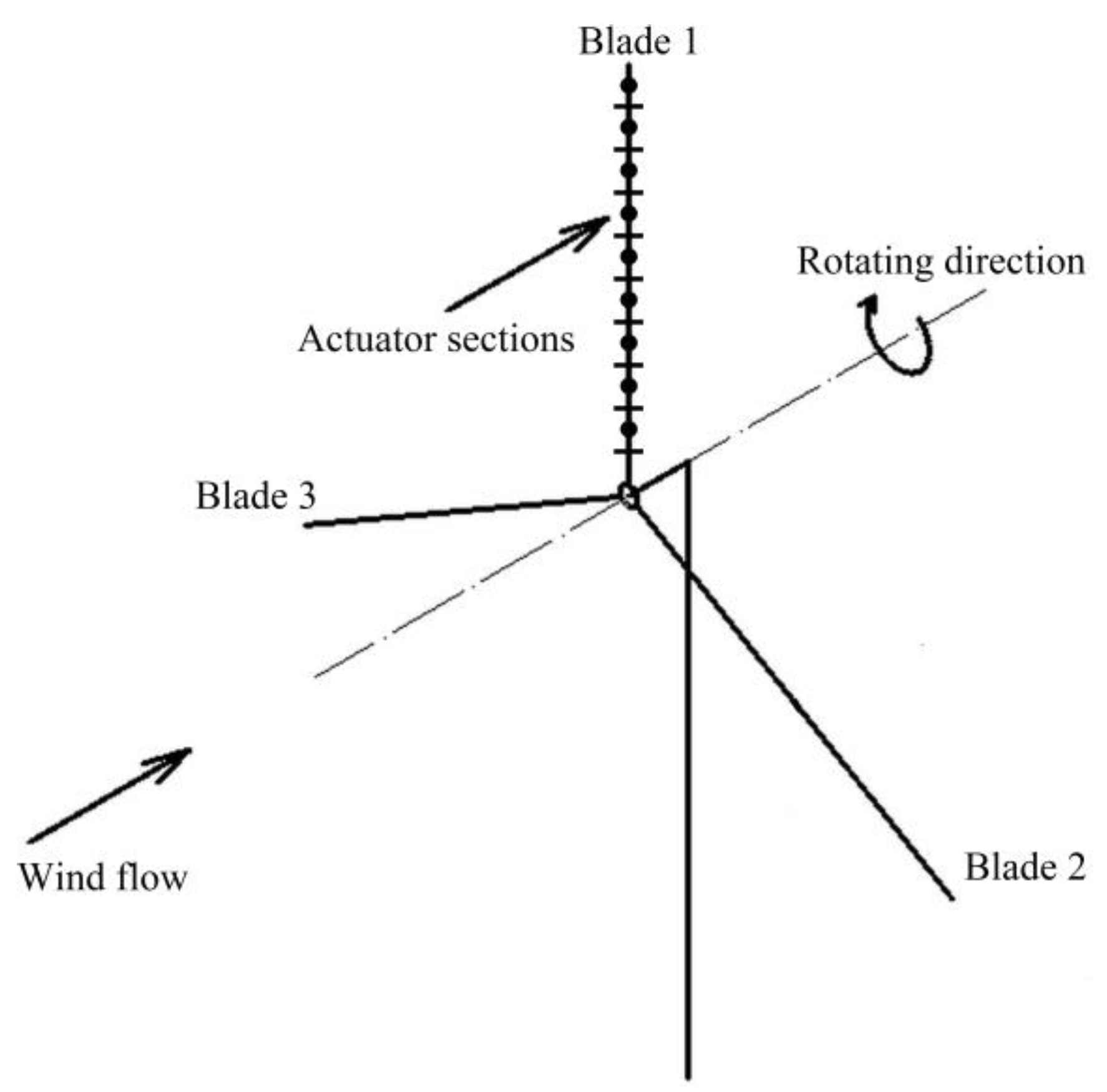
In the actuator line model, the blades of wind turbine are replaced by lines with the aerodynamic force distributed on it, as shown in Figure 1. The lines are discretized into actuator sections, in which there are different airfoils, chords and structure twists. The loading in each section, which is usually named as the aerodynamic force, can be calculated by Equation (1).

$$f=(L,D)=\frac{1}{2}\rho U^{2}c(C_l\overrightarrow{e_L}+C_d\overrightarrow{e_D})$$

(1)

where f is the aerodynamic force; L and D are lift and drag, respectively; ρ is the air density, and $\rho =1.225\hspace{0.17em}\mathrm{kg}/{\mathrm{m}}^3$ in this paper; U is the relative velocity of the blade element in actuator sections; c is the chord length; $C_l$ and $C_d$ are the coefficients of lift and drag, which can be looked up from airfoil data tables derived from physical experiment; $\overrightarrow{e_L}$ and $\overrightarrow{e_D}$ represent the unit direction vectors of L and D.

Besides, the aerodynamic loads are concentrated on the aerodynamic center of the blade element, which are located in 0.25 chord length. To describe the influence of wind turbine blade on the flow field, the aerodynamic loads should be dispersed on the grid point. There are many distributional ways, and three-dimensional Gaussian distribution ${\eta }_{\epsilon }$ is used in this paper, whose function is shown in Equation (2). This equation is a smooth function and can avoid numerical singularity.

$${\eta }_{\epsilon }(d)=\frac{1}{{\epsilon }^3{\pi }^{3/2}}\exp [-{(\frac{d}{\epsilon })}^2]$$

(2)

where ε is a constant to adjust the strength of the distribution formula, and it is two times of local grid scale in this study according to Shives [26]; and d is the distance between the force point and the grid point. Therefore, the forces $f_{\epsilon }$ on the nearby mesh can be calculated by Equation (3) and added into the momentum equation to solve the flow field as the body forces.

$$f_{\epsilon }=f\times {\eta }_{\epsilon }(d)$$

(3)

$$\frac{\partial V}{\partial t}+V\cdot \nabla V=-\frac{1}{\rho }\nabla p+\upsilon {\nabla }^{2}V+f_{\epsilon }$$

(4)

where V and p are the wind speed and pressure in the flow; $\upsilon$ is the kinematic viscosity, and it is set as $1.5\times {10}^{-5}\hspace{0.17em}{\mathrm{m}}^2/\mathrm{s}$; $f_{\epsilon }$ is the source item calculated through Equation (3).

Moreover, the Prandtl–Glauert tip loss model is used to the consideration that the velocity is zero at the tip. The function of tip loss model is shown as Equation (5).

$$F_{tip}=\frac{2}{\pi }\arccos [\exp (-\frac{B(R-r)}{2r\sin \varphi })]$$

(5)

where $F_{tip}$ is the aerodynamic corrected force at the tip; B is the blades number; R is the radius of the blades; r is the distance between the root of blades and the action point of aerodynamic force; and $\varphi$ is the angle between U and the rotor plane [27]. Tower and hub effect are also considered in this research by similar technology, and their airfoils are cylinder.

2.2. Rotating Beam Solver

The blades of wind turbine are considered as rotating variable cross-section projecting beams in this study. In this section, an approach of solving these beams in actual design is introduced [24]. Although this method is faulty and not suitable for structural solution, it still could catch some phenomena in vibration.

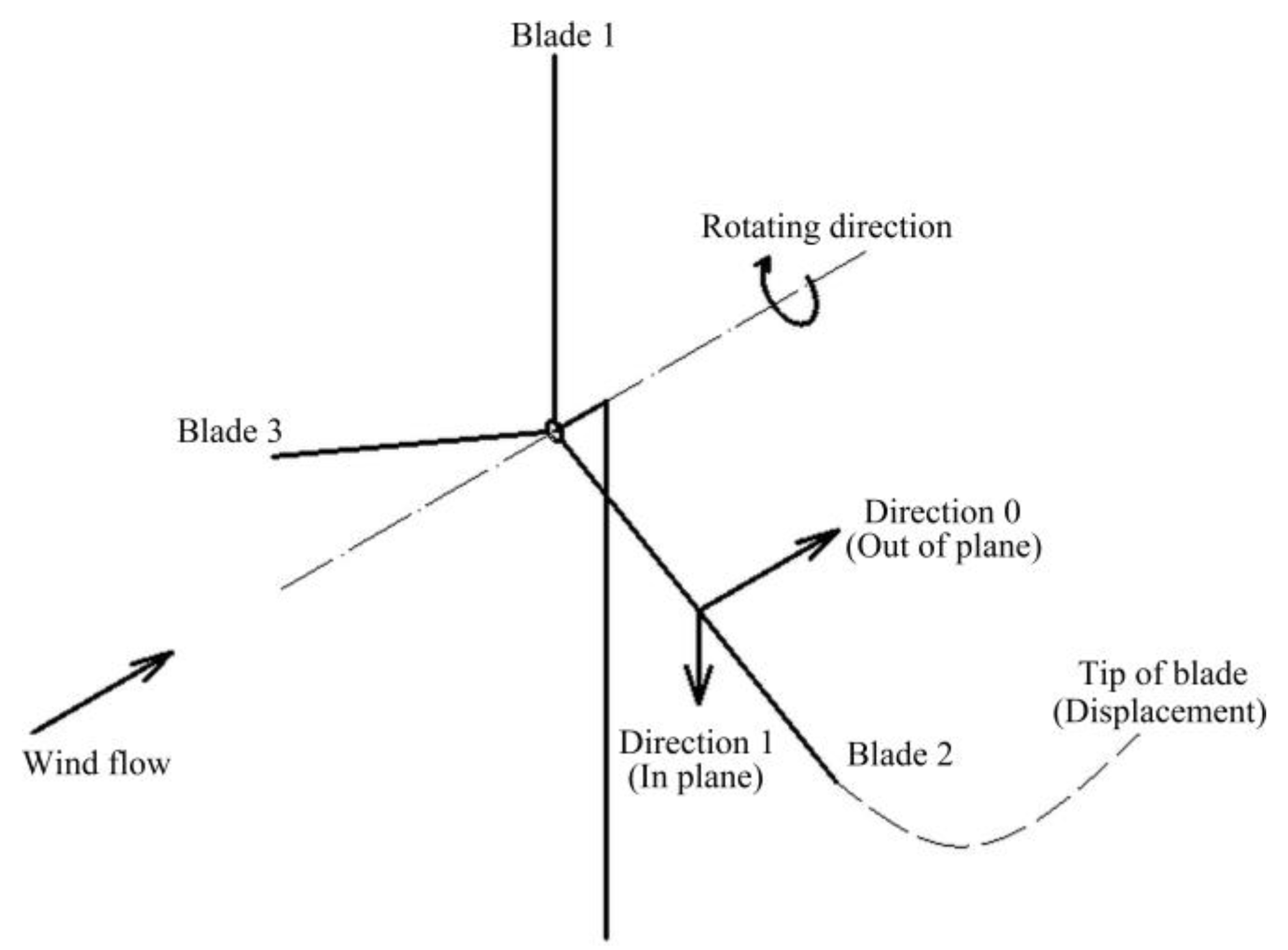
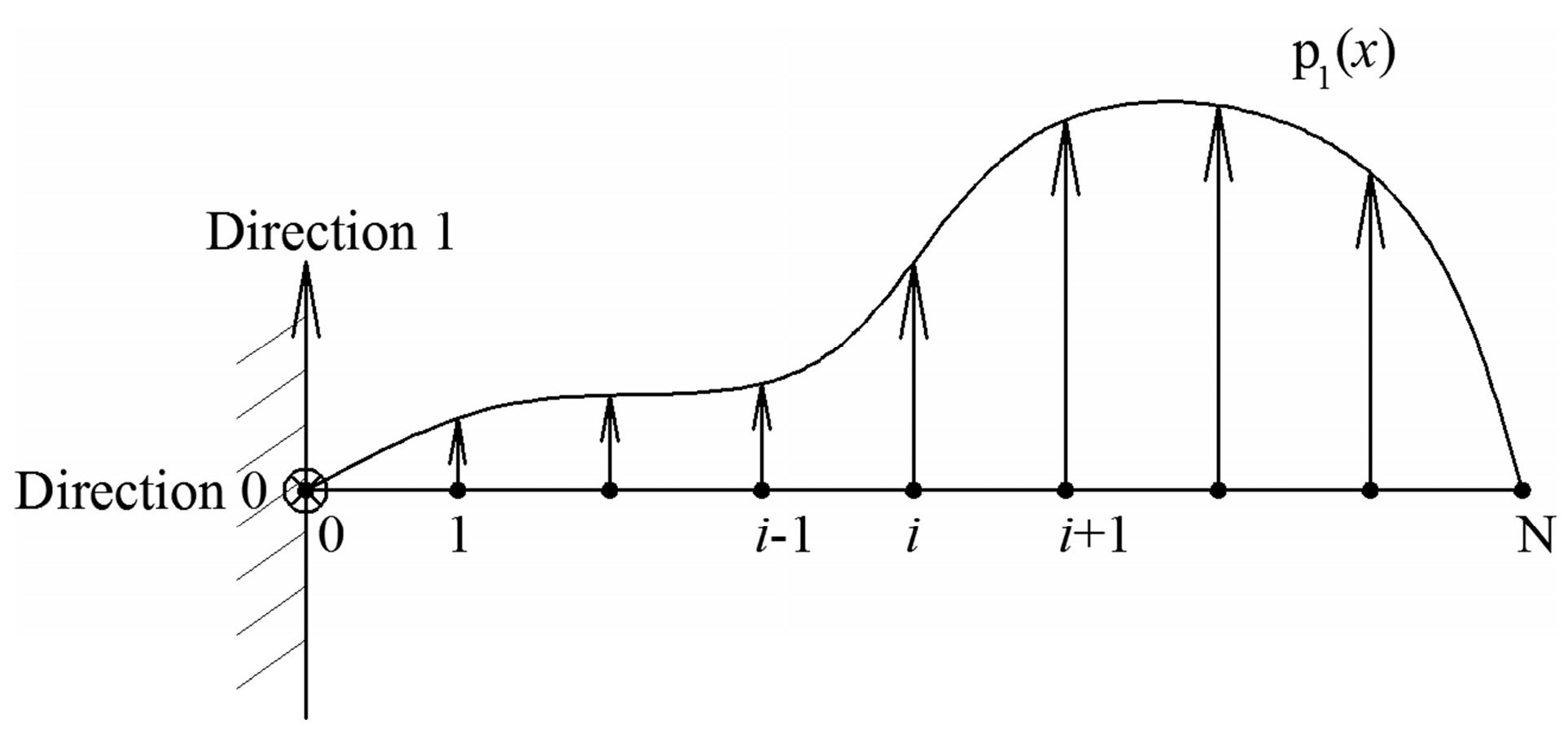
Figure 2 shows the diagram of the blade deflection, in which the blades have been substituted by actuator lines. In the picture, direction 0 is out of the rotating plane and called flapwise. Similarly, direction 1 is in the rotating plane and called edgewise. In this research, the subscript 0 means the component of the physical quantity in 0 direction and the subscript 1 represents component of the corresponding parameter in 1 direction. The diagrammatic sketch of the forces on the blade, which is considered as a cantilever beam, is given in Figure 3. According to the Newton’s second law of a microelement, the sheer stresses $T_0$, $T_1$ and the bending moments $M_0$, $M_1$ of each blade element can be calculated from Equation (6) to Equation (9).

$$\frac{d{T}_0}{dx}=-p_0(x)-m(x)g\sin \theta +m(x){\ddot{y}}_0(x)$$

(6)

$$\frac{d{T}_1}{dx}=-p_1(x)-m(x)g\cos \theta +m(x){\ddot{y}}_1(x)$$

(7)

$$\frac{d{M}_1}{dx}=T_0+N_0$$

(8)

$$\frac{d{M}_0}{dx}=-T_1+N_1$$

(9)

where p(x) is the aerodynamic force distribution; m(x) is the blade mass distribution; g is the gravitational acceleration, and it is set as 9.8 $\mathrm{m}/{\mathrm{s}}^2$ in this paper; $\theta$ is the shaft tilt angle, and it is 5 degree here; $\ddot{y}$ is the displacement y to the second derivative of time, and it can be calculated by prediction and correction of modified Euler method, given from Equation (10) to Equation (13); N₀, N₁ are the component of centrifugal force in 0 direction and 1 direction.

$${\tilde{y}}_{n+1}=2y_n-y_{n-1}+{\ddot{y}}_{n}dtdt$$

(10)

$${\tilde{\ddot{y}}}_{n+1}=h\left({\tilde{y}}_{n+1},t_{n+1}\right)$$

(11)

$$y_{n+1}=2y_n-y_{n-1}+0.5({\ddot{y}}_n+{\tilde{\ddot{y}}}_{n+1})dtdt$$

(12)

$${\ddot{y}}_{n+1}=h\left(y_{n+1},t_{n+1}\right)$$

(13)

where the subscript n + 1 represents at time $t_{n+1}$; the subscript n represents at time $t_n$; $\tilde{y}$ is predicted value; function h can be calculated from transposition of structure equations, as shown in Equation (15).

$$M(x)\ddot{y}+K(x)y=F(x,t)$$

(14)

$$\ddot{y}=\frac{F(x,t)}{M(x)}-\frac{K(x)y}{M(x)}=g(y,t)$$

(15)

where Equation (14) is the structure equations without damping; $M(x)$ is mass of blade; $K(x)$ is the stiffness of blade; $F(x)$ is the external loading.

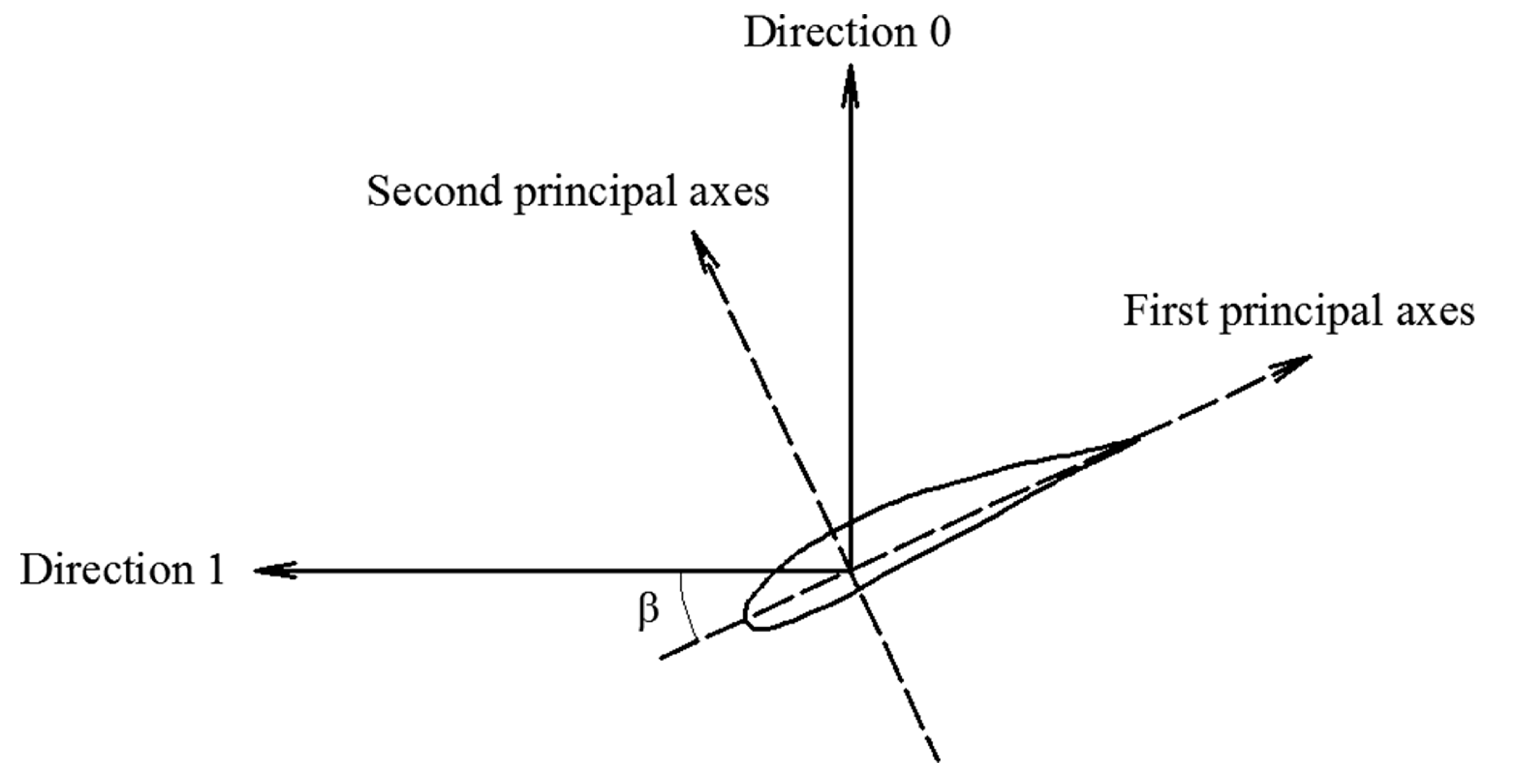
According to Figure 4, the bending moments $M_0$ and $M_1$ can be transformed into principal axes direction by Equation (16) and Equation (17).

$$M_{11}=M_1\cos \beta -M_0\sin \beta$$

(16)

$$M_{22}=M_1\sin \beta -M_0\cos \beta$$

(17)

where $M_{11}$ and $M_{22}$ are the bending moments on the first principal axis and the second principal axis; $\beta$ is the structure twist angel.

Based on the beam theory, the curvature of principal axes ${\kappa }_{11}$ and ${\kappa }_{22}$ can be obtained from Equation (18) and Equation (19).

$${\kappa }_{11}=\frac{M_{11}}{E{I}_1}$$

(18)

$${\kappa }_{22}=\frac{M_{22}}{E{I}_2}$$

(19)

where EI is the stiffness of the blade element.

Equation (18) and Equation (19) are converted back to direction 0 and direction 1 through the formulas as following:

$${\kappa }_0=-{\kappa }_{11}\sin \beta +{\kappa }_{22}\cos \beta$$

(20)

$${\kappa }_1={\kappa }_{11}\cos \beta +{\kappa }_{22}\sin \beta$$

(21)

Therefore, the angular deformation $\theta$ and deflection y can be calculated by:

$$\frac{d{\theta }_1}{dx}={\kappa }_1$$

(22)

$$\frac{d{\theta }_0}{dx}={\kappa }_0$$

(23)

$$\frac{d{y}_0}{dx}=-{\theta }_1$$

(24)

$$\frac{d{y}_1}{dx}={\theta }_0$$

(25)

The root of the blade is clamped, so the boundary condition at root is:

$${\theta }_0=0,{\theta }_1=0,y_0=0,y_1=0$$

(26)

The tip is free end, so the boundary condition at tip is:

$$T_0=0,T_1=0,M_0=0,M_1=0$$

(27)

2.3. New Elastic Actuator Line Model

In this section, the ALM is improved into a new elastic actuator line model (EALM) based on turbinesFoam library, which is developed by Bachant et al. [25]. This library uses ALM to simulate wind and marine hydrokinetic turbines in OpenFOAM. Its interpolation, Gaussian projection, and vector rotation functions are all adapted from NREL’s Simulator for Off/Onshore Wind Farm Applications (SOWFA).

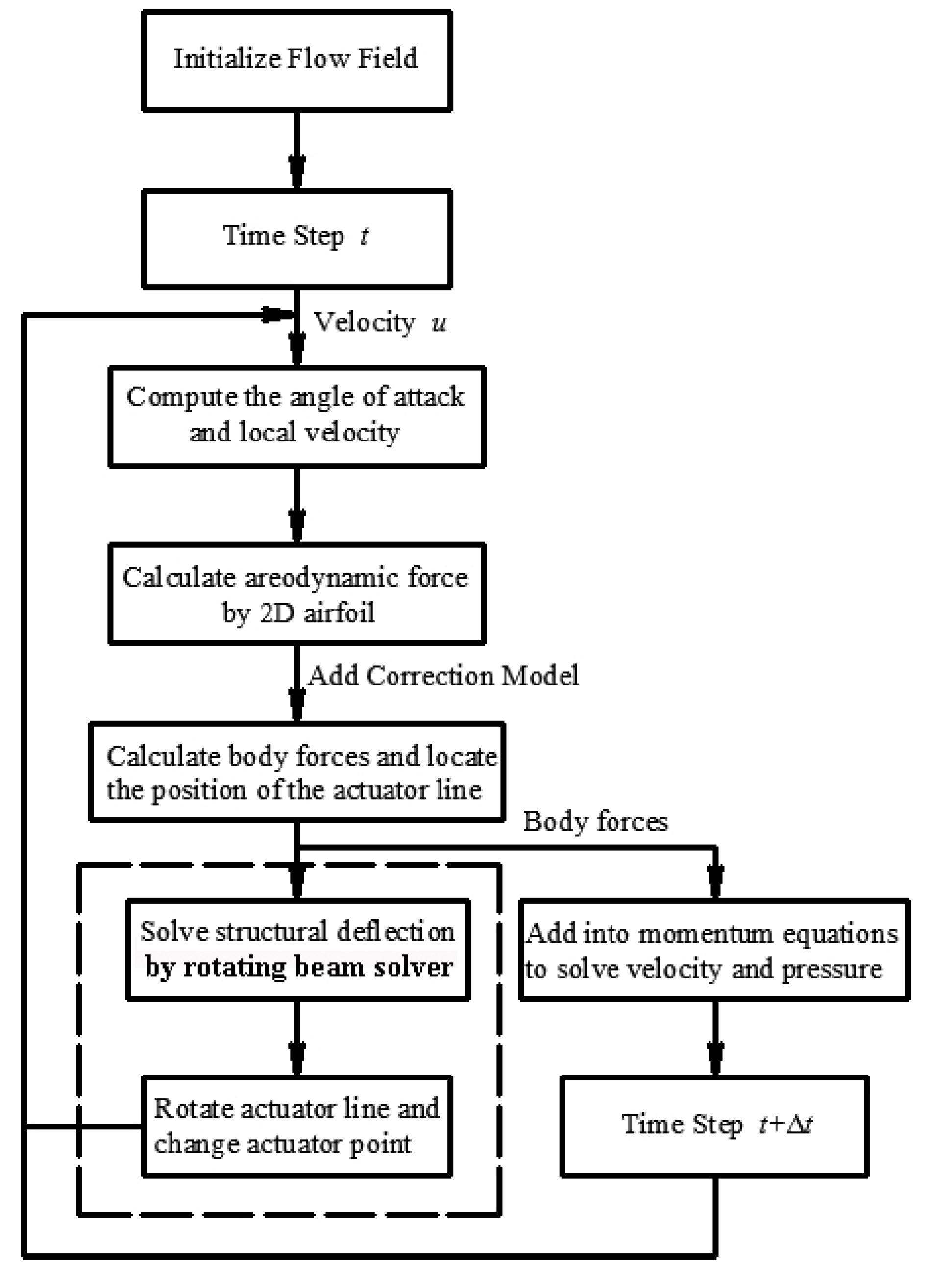
In EALM, the body forces are calculated by traditional ALM and the blade deflection is computed by rotating beam solver, which is defined in Section 2.2. The computation process of EALM is given in Figure 5, in which the difference between EALM and ALM is marked by dashed rectangle. The part of structure solver is added into the actuatorLineSource class, and the actuator point is changed in the actuatorLineElement class. From Figure 5, it can be found that this combination of ALM and structure model is one-way coupling. Compared with the research by Meng et al. [23], the part of aerodynamics solver is similar, but the way of dealing with structural solver is different (see Section 2.2). The advantages of this model are that the EALM allows large time step when the position of actuator line changes every time and computes long terms of wind turbine working. This technology will be further improved and used in the simulation of the floating offshore wind turbine in the sea, which needs more simulation time to keep the floating foundation stability under waves.

2.4. Computational Wind Turbine Model

In this study, the aerodynamic performances, which are power and thrust, and the structural responses, which are represented mainly by the blade tip displacement, will be compared with different research using varieties methods to validate EALM. According to the theory above, all these three physical quantities are obtained from the aerodynamic forces along the blade. Different cases use varieties method to achieve these forces. Only if the blade properties, including the aerodynamic and structural properties, and the computational condition such as wind speed are all the same, these three quantities could make equivalent comparisons. Thus, the computational condition will be given next. The model used in this research is NREL 5 MW wind turbine, and its gross properties are listed in

Table 1. Properties of NREL 5 MW baseline wind turbine (NREL: National Renewable Energy Laboratory).

Properties	Content
Rotor orientation	Upwind
Rotor configuration	Three blades
Rotor diameter	126 m
Hub diameter	3 m
Hub height	90 m
Shaft tilt angle	5°
Rotor mass	110,000 kg
Rated power	5 MW
Rated wind speed	11.4 m/s
Rated rotor speed	12.1 rpm

. The details of the blade structural and aerodynamic properties can be referenced in Jonkman’s technical report [8]. To be exact, the shaft tilt angle is considered in the structural part, which will make the external force of blade increased because of the gravity component.

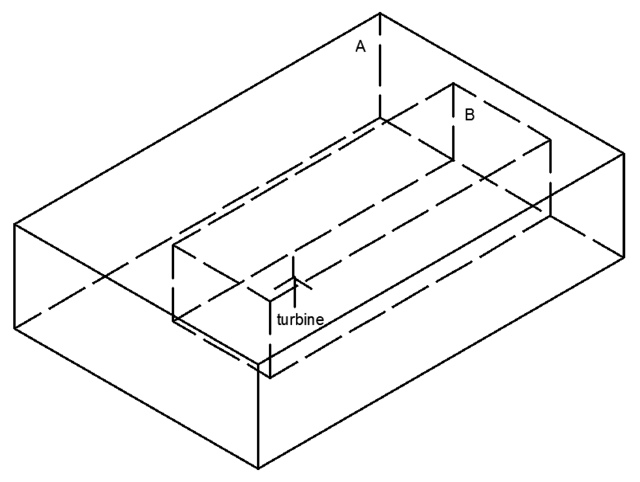
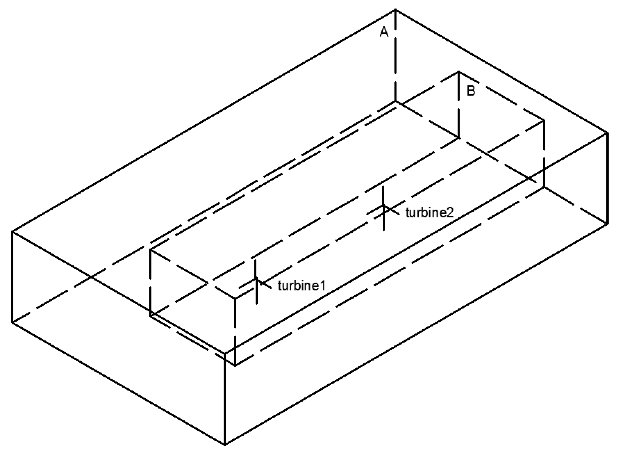
The simulation physical domains used in this paper are the same as Yu et al. [28]. Their three-dimensional sketches are shown in Figure 6 and Figure 7. In these pictures, A is the outer mesh region and B is the refined mesh region, where the grid is refined by 4 levels. The mesh refined ratio is 0.5 between each level. The mesh independence test has been completed in that research and 1.5 m is chosen as the minimum size of grid. Besides, it is confirmed that the wind turbine gets a better working status at the wind speed of 8 m/s and its corresponding tip speed ratio is 7.55. As a consequence of this model, the cases studied in present research are mainly in two situations, 8 m/s and 11.4 m/s. To analyze the aeroelastic performance in the wake, double NREL 5 MW wind turbines set in a line are studied, and its simulation domain is shown in Figure 7. The main contents of this research are focused on the downstream wind turbine.

Compared to the work of Yu et al. [28], the parameter settings are all the same expect that the LES (Large Eddy Simulation) model is used instead of RANS (Reynolds Average Navier-Stokes). That is because the LES model will get more accurate results about the vorticities than RANS and the influence of the wake flows to elastic blade is studied in this research. In addition, the wind turbine blade deflection solver is added in ALM, named EALM.

3. Verification and Analysis

In this section, the mesh independence and uncertainty analysis of actuator point number are given first. Then, the aerodynamic performance and the structural responses are compared to validate EALM. The aerodynamic performance contains the power and the thrust. The structural responses are represented mainly by the blade tip displacement.

3.1. Mesh Independence and Uncertainty Analysis

Four levels of grids are tested to prove the mesh independence under the rated wind speed, and the non-dimension coefficients of power and thrust are compared in

Table 2. Mesh independence test of power and thrust coefficient.

Grid Level	Number of Cell	Size of Wake Region Cell (m)	Cp	Ct
1	0.38 M	2.5	0.4678	0.8665
2	0.75 M	2.0	0.4642	0.8599
3	2.90 M	1.5	0.4634	0.8584
4	5.96 M	1.0	0.4627	0.8572

. They are defined as power coefficient C_p and thrust coefficient C_t as below:

$$C_p=\frac{P}{0.5\rho V^3\pi R^2}$$

(28)

$$C_t=\frac{T}{0.5\rho V^3\pi R^2}$$

(29)

where P is the mechanical power; ρ is the air density; V is the wind speed in the flow; T is the thrust on the blades. It shows that the results drop slow when the grid levels up especially from level 3 to level 4. Therefore, the level 3 mesh is used in the following research.

According to Shives’ research [26], the number of actuator point has the rule that the maximum of the distance between the adjacent point should not more than the size of blade region. Different actuator point numbers are also tested in

Table 3. Relationship between actuator point number and aerodynamic coefficients.

Level	Actuator Point Number	Cp	Ct
1	54	0.4650	0.8608
2	72	0.4634	0.8584
3	90	0.4632	0.8580

and Figure 8. Besides, the mesh size and computational condition are kept as constant during this test. To improve the accuracy the uncertainty coefficient $U_{\xi }$ is calculated as follow steps.

(1) Calculate the difference of aerodynamic coefficients between neighbor level, which are defined as ${\epsilon }_{\zeta 21}$ and ${\epsilon }_{\zeta 32}$;

(2) The convergence ratio $R_{\xi }$ can be computed by Equation (30).

$$R_{\xi }=\frac{{\epsilon }_{\zeta 32}}{{\epsilon }_{\zeta 21}}$$

(30)

(3) The power coefficient convergence ratio is 0.125 and the thrust coefficient convergence ratio is 0.167. They are both located in the interval which greater than 0 and less than 1. So, the Richardson extrapolation method is used to get the order of accuracy $p_{\xi }$ and the estimated value of error ${\delta }_{\mathrm{Re}\xi 1}$ in Equation (31) and Equation (32).

$$p_{\xi }=\frac{\ln ({\epsilon }_{21}/{\epsilon }_{32})}{\ln (r_{\xi })}$$

(31)

$${\delta }^{*}{}_{\mathrm{Re}\xi 1}=\frac{{\epsilon }_{\xi 32}}{r_{\xi }^{p_{\xi }}-1}$$

(32)

where $r_{\xi }$ is refinement ratio of actuator point number.

(4) The uncertainty coefficient $U_{\xi }$ can be compute by Equation (33).

$$U_{\xi }=(\left|C_{\xi }\right|+\left|1-C_{\xi }\right|)\left|{\delta }^{*}{}_{\mathrm{Re}\xi 1}\right|$$

(33)

where $C_{\xi }$ is correction factor and defined by Equation (34).

$$C_{\xi }=\frac{r_{\xi }^{p_{\xi }}-1}{r_{\xi }^2-1}$$

(34)

Following the calculation steps above, the uncertainty coefficient of C_p and C_t can be achieved. They are 0.129% D and 0.126% D, where D is the reference data from the NREL technical report [8]. Because both of them are less than 1% D, that proves the results are credible. Through the verification above, the level 2 actuator point number will be adopted, and it will obtain reliable results.

In addition, one of this method’s advantages is that in the part of the aerodynamic solver it will cost less computational resources than CFD. The BEM theory is not considered here because the wake flow cannot be achieved in this way. The comparison of the computational cost between ALM and CFD method are shown in

Table 4. Comparison of the computational cost between actuator line method (ALM) and computational fluid dynamics (CFD) method.

Method	Software	Number of Cell	Simulated Time	Power
ALM	OpenFOAM	1.49 M	9.2 h	5.036 MW
CFD	Star CCM+	5.01 M	82.0 h	5.050 MW

ALM: Actuator Line Method; CFD: Computational Fluid Dynamics; OpenFOAM: Open Source Field Operation and Manipulation, a free, open source CFD software package released by the OpenFOAM Foundation, which was incorporated as a company limited by guarantee in England and Wales; Star CCM+: Siemens Digital Industries Software, 5800 Granite Parkway, Suite 600, Plano, TX, USA.

. It can be concluded that ALM uses less grids and computes faster than the CFD method under similar accuracy.

3.2. Comparison of the Power and the Thrust

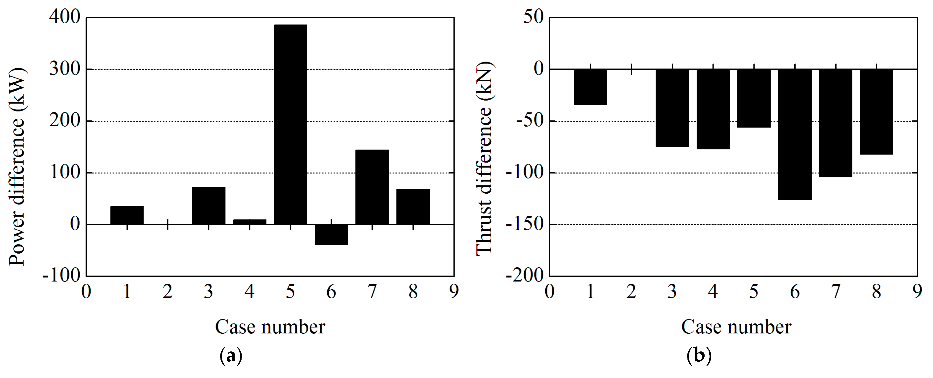
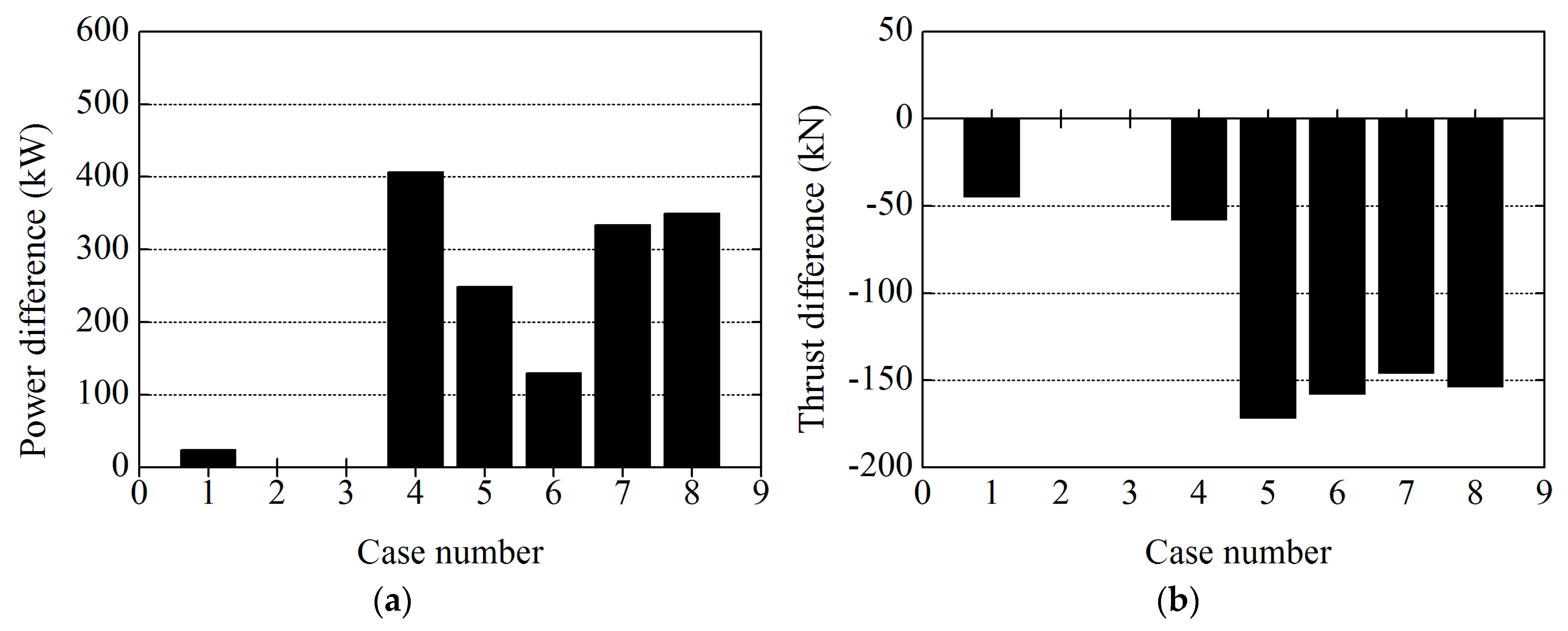
In this part, the results of aerodynamic performance are compared with 8 cases, in which 7 cases are the previous research and 1 case is the present one. Case 1 is the simulation of EALM and it is the present study. Case 2 is from the official technical report even though some data are given by NREL’s FAST code [8]. In this report, the blade mode is derived by the mode’s program and then passes a best-fit polynomial to get the equivalent polynomial representations of the mode shapes needed by FAST. Case 3 is simulated by HAWC2 (Horizontal Axis Wind turbine simulation Code 2nd generation) [29], which is an in-house nonlinear aeroelastic model developed by Technical University of Denmark. BEM is used as aerodynamic model and the multi-body dynamics method (MBD) is its structural model, in which each body is a linear Timoshenko beam element. The data of Case 4 are calculated by Li et al. [17] using CFD and MBD. This approach uses a dynamic overset CFD code for aerodynamics and MBD code for motion responses. The coupled way is done by exchanging the information between the fluid and structure solver in explicit form. The results of Case 5 are given by Jeong et al. [30] with BEM. In their research, the FSI (Fluid–Structure interaction) applies a strong coupling method which is using a first order implicit-explicit coupling scheme. Case 6 is set up in the research of Ponta et al. [31] by BEM and dynamic rotor deformation model, where the effects of rotor deformation are incorporates in the computation of aerodynamic loads. Yu et al. [32,33] combined CFD and CSD (Computational Structural Dynamics) in Case 7. The coupling methodology in this research is made by adopting the delta-airload loose-coupling technology. The last Case 8 is the results of the actuator line finite-element beam method (ALFBM) by Ma et al. [13]. The process of this research is three parts: the CFD solver given by OpenFOAM, the aerodynamic solver calculated by ALM, and the structural solver by finite-element beam method. The coupled steps are reading the velocity in the flow field from t–Δt and adding it to source term, which is computed by aerodynamic solver and structural solver. To clearly compare the varieties, the detailed information about the solved method on the aerodynamic performance and the structural responses in different cases are given in

Table 5. Detailed information about the solved method on the aerodynamic performance and the structural responses in different cases.

Case Number	Aerodynamic Method	Elastic Dynamics Method	Studying Contents
1	ALM	Rotating beam solver	Variation in wake flow
2	BEM	Modal approach	Blade response and aerodynamics
3	BEM	MBD	Blade response and aerodynamics
4	CFD	MBD	Influence of wind turbulence
5	BEM	Geometric nonlinearity beam model	Optimal yaw and pitch angle
6	BEM	Dynamic rotor deformation model	Rotor structure deformation
7	CFD	FEM-based CSD beam solver	Yaw and wind shear
8	ALM	Finite-element beam method	Wake behavior

ALM: Actuator Line Method; BEM: Blade-Element Momentum; MBD: Multi-Body Dynamics; CFD: Computational Fluid Dynamics; CSD: Computational Structural Dynamics; FEM: Finite Element Method.

. In this research, BEM theory cannot describe the detailed flow field, and the CFD method may cost too much time to calculate. Therefore, ALM is chosen to resolve aerodynamic performance. Compared to ALFBM, this research concentrates on the variation of the aeroelastic characteristics in wake flow caused by upstream wind turbine.

Table 6. Comparison of the power and the thrust with different research.

Case Number	8 m/s		11.4 m/s
	Power (MW)	Thrust (kN)	Power (MW)	Thrust (kN)
1	1.891	432	5.024	772
2	1.856	466	5.000	817
3	1.928	391	No data	No data
4	1.865	389	5.407	759
5	2.242	410	5.249	645
6	1.817	340	5.130	659
7	2.000	362	5.334	671
8	1.924	384	5.350	663

Case 1: Elastic Actuator Line Model (present study); Case 2: NREL’s Fatigue, Aerodynamics, Structures, and Turbulence (FAST) code; Case 3: Horizontal Axis Wind turbine simulation Code 2nd generation results; Case 4: research by Li et al. [17]; Case 5: research by Jeong et al. [30]; Case 6: research by Ponta et al. [31]; Case 7: research by Yu et al. [32,33]; Case 8: research by Ma et al. [13].

lists the results of 8 cases with velocities of 8 m/s and 11.4 m/s, and their mean output power and thrust differences are described in a histogram to visualize disparity of these cases, as shown in Figure 9 and Figure 10. According to the results, the NREL’s reported results are chosen as the reference data. It can be seen that all the results of power are higher than the reference data, except Case 6. All the results of thrust are lower than the FAST result. The big difference of thrust results are found from Case 5 to Case 8. The main reason for this is that the tip loss correction is not considered, and it has a great influence on aerodynamic performance. Case 4 has unsatisfied power result and there is no data in Case 3 under the rated situation. Besides, Case 1 has the most approximate result to the reference data among all studies. Its power difference is less than 50 kW and thrust difference is not more than 50 kN.

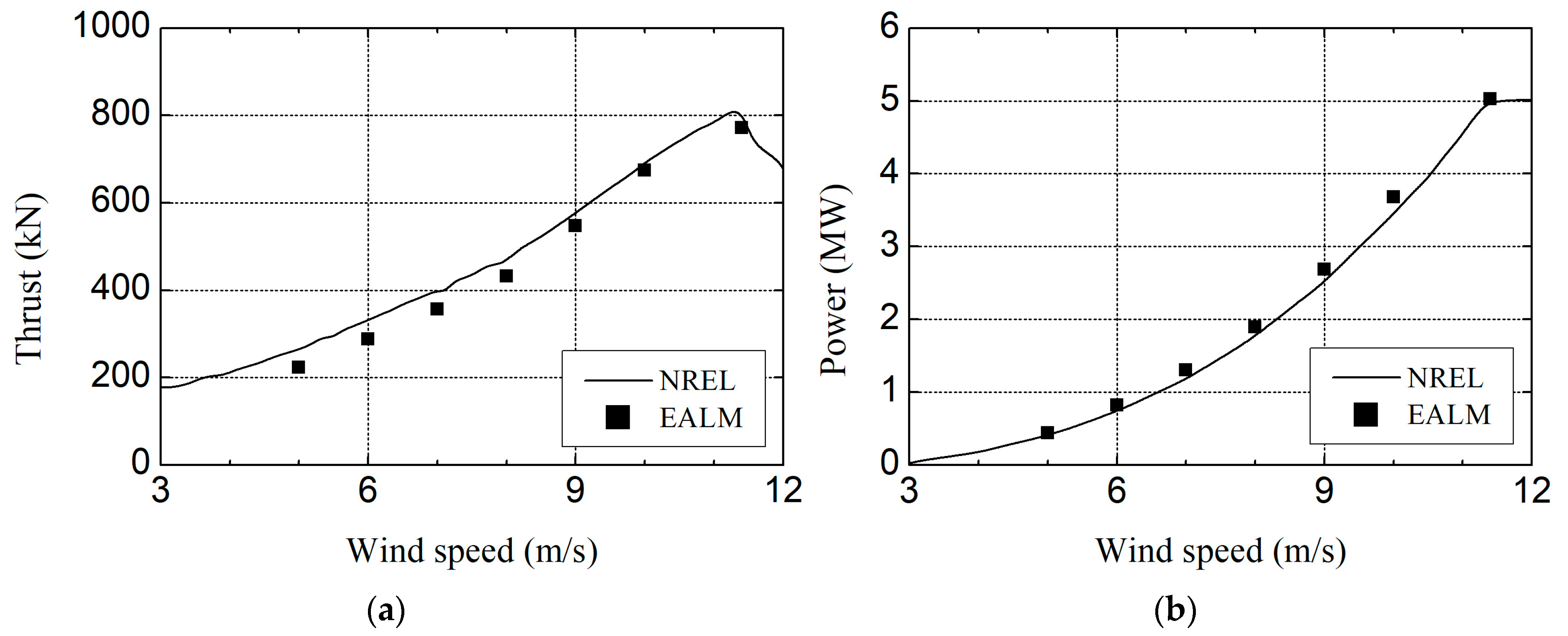
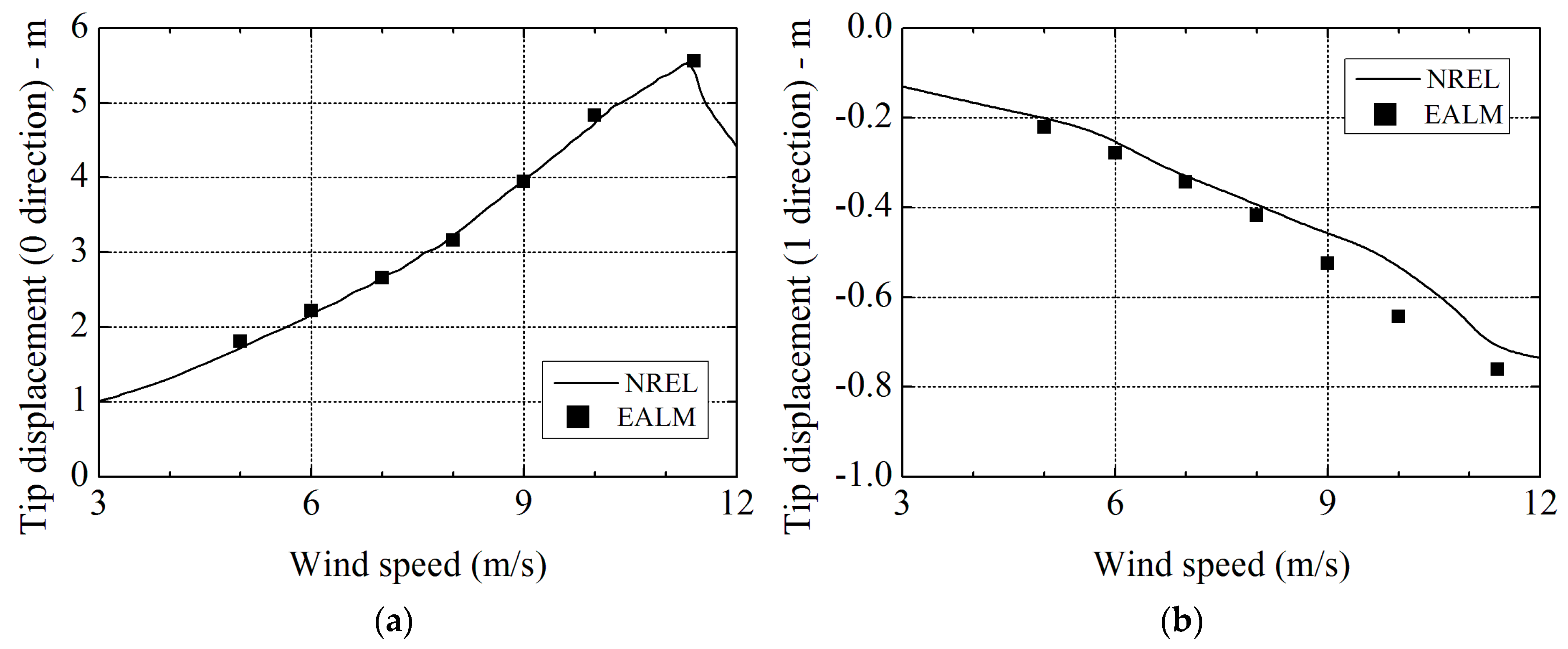
To further examine the accuracy of EALM under different wind speed conditions, power and thrust are computed and compared with Case 2, which are shown in Figure 11. Besides, their relative errors are given in

Table 7. Comparisons of the power and the thrust relative error between elastic actuator line model (EALM) and NREL’s FAST code at different wind speeds.

Wind Speed (m/s)	Power (MW)	Error	Thrust (kN)	Error
5.0	0.4355	2.828%	222.6153	15.965%
6.0	0.8194	7.080%	287.8339	13.253%
7.0	1.2986	6.099%	356.5589	10.233%
8.0	1.8906	3.856%	432.3593	7.543%
9.0	2.6880	3.564%	546.8937	5.374%
10.0	3.6799	3.405%	674.6184	2.392%
11.4	5.0241	0.482%	772.1718	3.948%

. The errors are smaller when the wind speed is close to the rated speed, which is 11.4 m/s, than those when the wind speed is below 8 m/s. This phenomenon is caused by the coefficients of lift and drag $C_l$ and $C_d$ in Equation (1). These two parameters are referenced from airfoil data tables and these tables are achieved by physical experiment which is given by NREL official report [8]. In that report, the airfoil data is only obtained under nearly rated wind speed. Therefore, the lift and drag of a blade element can get more accurate if the wind speed closed to 11.4 m/s. On the contrary, the result of the force in the blade element will not be satisfactory if the wind speed is far away from 11.4 m/s. In case of application that the airfoil data corresponds to the wind speed, the result will be perfect, which will be improved in future research. From results of Picture 11, the predict results show good agreements with NREL’s reference data. In addition, the differences between NREL and EALM are getting small with the inlet wind velocity increasing whether the output power or thrust. Especially in the rated situation, the relative errors of both power and thrust are less than 5%.

According to the validation above, it could be concluded that EALM can predict the power and thrust accurately. This conclusion can be predictable because the aerodynamic calculations of EALM are based on blade element theory. In this theory, the lift and drag of blade element are achieved from two-dimensional airfoil data, which is obtained from physical experiments.

3.3. Comparison of the Tip Displacement

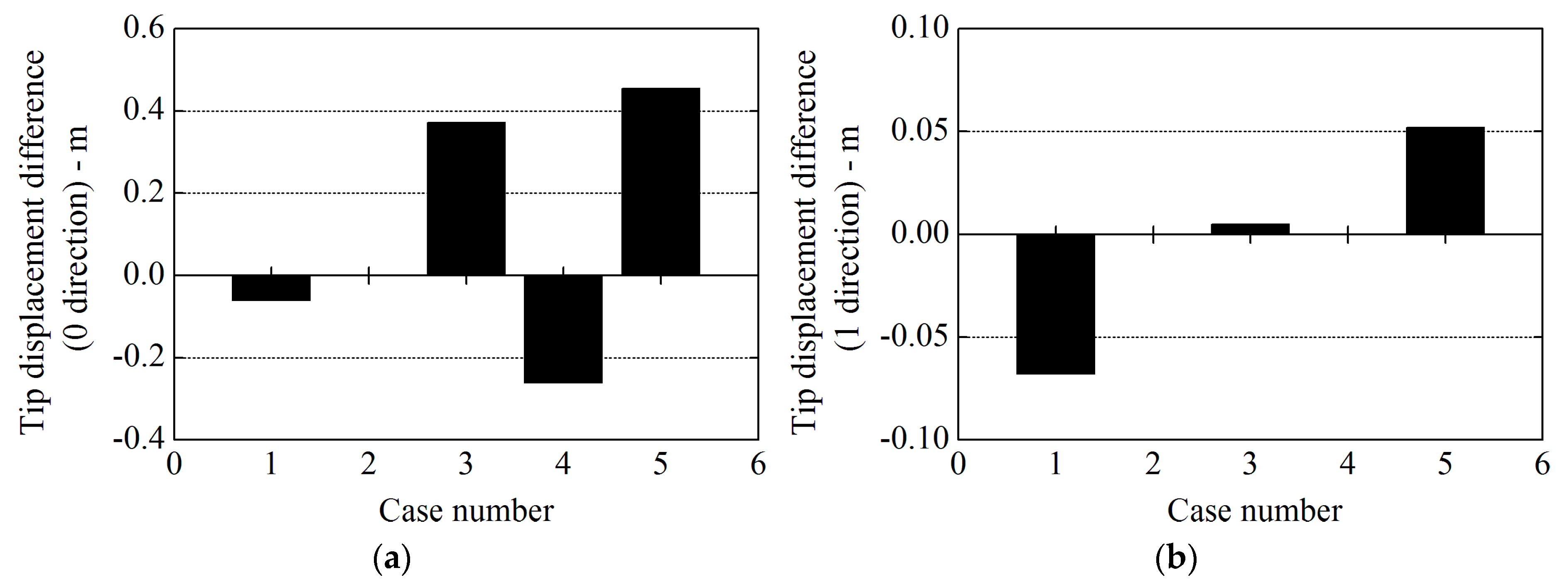
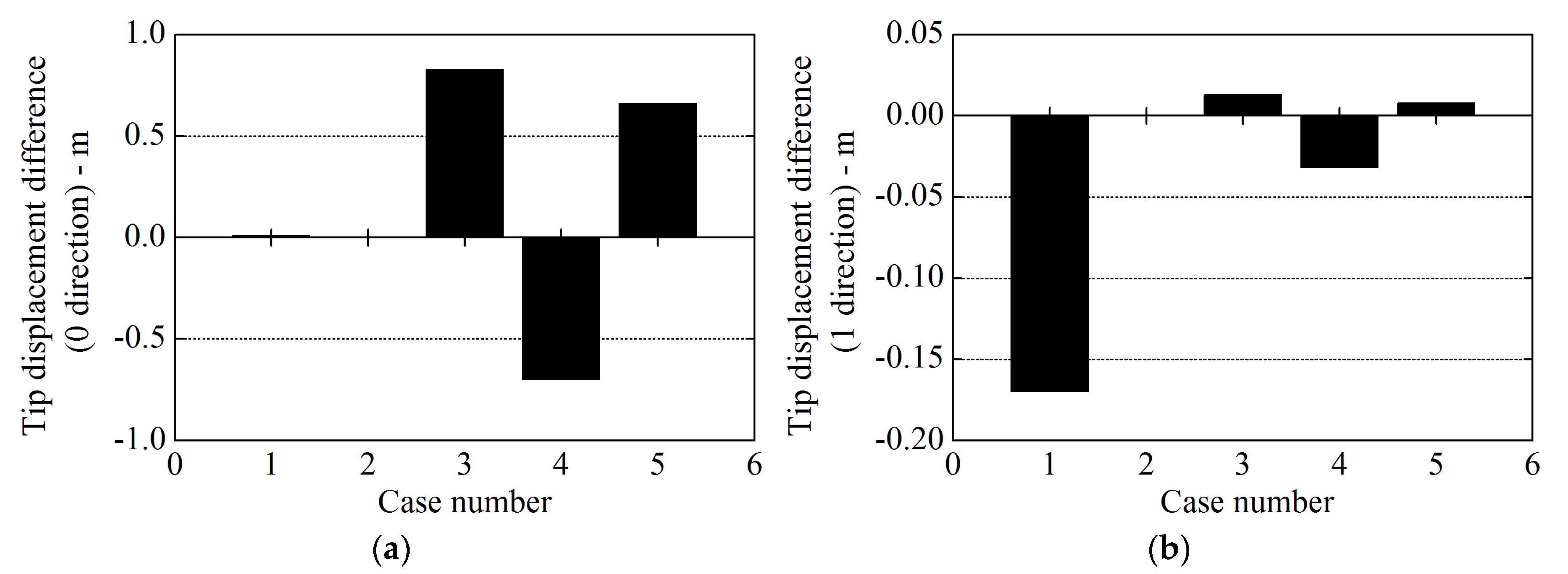
In this section, the structural responses of blade tip are compared in 5 cases. Case 1 is the present research and obtained by EALM. Case 2 is from the official technical report and its data are given by NREL’s FAST code [8]. Case 3 is the results of CFD and multi-body dynamics method by Li et al. [17]. Case 4 is set up by Yu et al. [32,33], in which CFD and CSD (Computational Structural Dynamics) are combined to calculate the coupled problem. The last Case 5 is using the actuator line finite-element beam method (ALFBM) by Ma et al. [13]. Detailed information in different cases can refer to Table 5.

Similarly,

Table 8. Comparison of tip deflection with different research.

Case Number	8 m/s		11.4 m/s
	Out of Plane Tip Displacement (m)	In Plane Tip Displacement (m)	Out of Plane Tip Displacement (m)	In Plane Tip Displacement (m)
1	3.159	−0.418	5.560	−0.762
2	3.220	−0.350	5.550	−0.592
3	3.592	−0.345	6.379	−0.579
4	2.958	No data	4.851	−0.624
5	3.675	−0.298	6.212	−0.584

Case 1: Elastic Actuator Line Model (present study); Case 2: NREL’s FAST code; Case 3: research by Li et al. [17]; Case 4: research by Yu et al. [32,33]; Case 5: research by Ma et al. [13].

lists the tip displacement results of 5 cases with 8 m/s and 11.4 m/s, and their differences are provided in the form of histograms, which are shown in Figure 12 and Figure 13. Additionally, the NREL’s reported results are chosen as the reference data. In these pictures, 0 direction means out of the rotor plane and 1 direction is in the rotor plane. The results of Case 3 and Case 5 are larger than those in Case 2, while the results of Case 4 are smaller. At the same time, the tip displacement of Case 1 is the nearest with the reference data in 0 direction and the farthest away from that reference data in 1 direction among 5 cases. It indicates that the tip displacement calculated by the beam solver, used in actual design, is similar to the modal approach, used to achieve structural dynamic characteristics, in 0 direction. Besides, the means used in this research could only predict approximate results in 1 direction. Even so, this beam solver can be still utilized to provide structural responses because of little deflection in edgewise.

The tip displacement and its relative error in varied wind speeds are compared with Case 2 in Figure 14 and

Table 9. Comparison of the tip displacement relative errors between elastic actuator line model (EALM) and NREL’s FAST code at different wind speeds.

Wind Speed (m/s)	Out of Plane Tip Displacement (m)	Error	In Plane Tip Displacement (m)	Error
5.0	1.8092	5.340%	−0.2215	−10.536%
6.0	2.2194	2.598%	−0.2793	−8.828%
7.0	2.6592	0.345%	−0.3437	−3.692%
8.0	3.1594	2.090%	−0.4177	−4.895%
9.0	3.9490	0.596%	−0.5247	−14.135%
10.0	4.8308	2.069%	−0.6441	−20.776%
11.4	5.5591	2.545%	−0.7616	−3.225%

. The predict tendency of the tip displacement in 0 direction is almost the same as the reference data from Figure 13a, and its relative error is less than 5%. That indicates once again that the result of beam solver used in this study is approximate to that of the modal approach in 0 direction. Although the predicted value is not satisfied in high wind velocity in 1 direction, the relative differences are still not more than 15% except in the velocity of 10 m/s.

To represent the exactitude of blade tip deformation in different positions when considering the rotating motion, the azimuthal variations of tip displacement are compared with FAST code in Figure 15 and Figure 16. In addition, the Pearson simplified correlation coefficient r is introduced to describe the fit degree of two curves. It is a measure of the linear correlation between two variables in statistics. It has a value from −1 to +1, where 1 is total positive linear correlation, 0 is no linear correlation, and −1 is total negative linear correlation. Moreover, the larger the absolute value of the correlation coefficient is, the stronger proximity of two variables becomes. In this study, the coefficient r is rearranged in the formulas like Equation (35).

$$r=\frac{n{\displaystyle \sum _{i=1}^n{x}_i{y}_i-{\displaystyle \sum _{i=1}^n{x}_i}}{\displaystyle \sum _{i=1}^n{y}_i}}{\sqrt{n{\displaystyle \sum _{i=1}^n{x}_i{}^2-{({\displaystyle \sum _{i=1}^n{x}_i})}^2}}\sqrt{n{\displaystyle \sum _{i=1}^n{y}_i{}^2-{({\displaystyle \sum _{i=1}^n{y}_i})}^2}}}$$

(35)

where n is sample size; $x_i$ and $y_i$ are the individual sample points indexed with i, and they represent the data from FAST and EALM in this research.

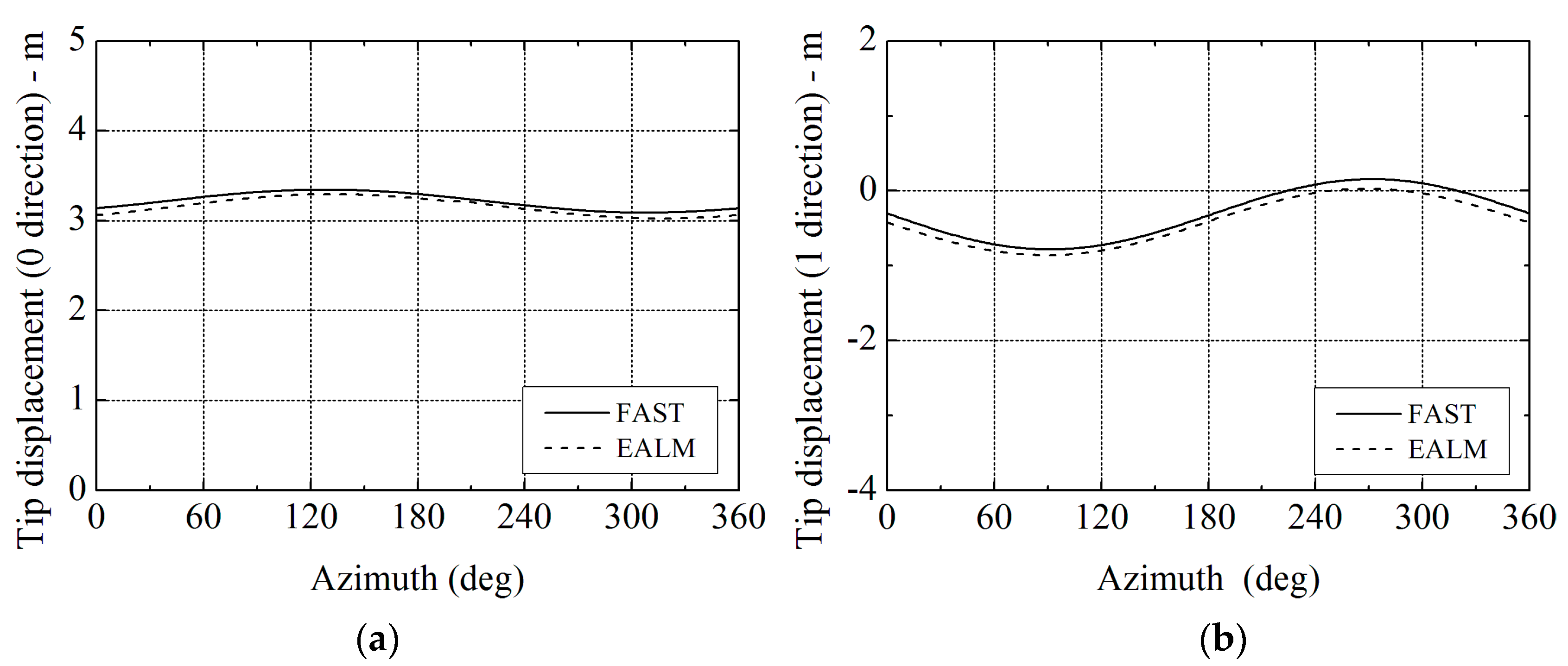
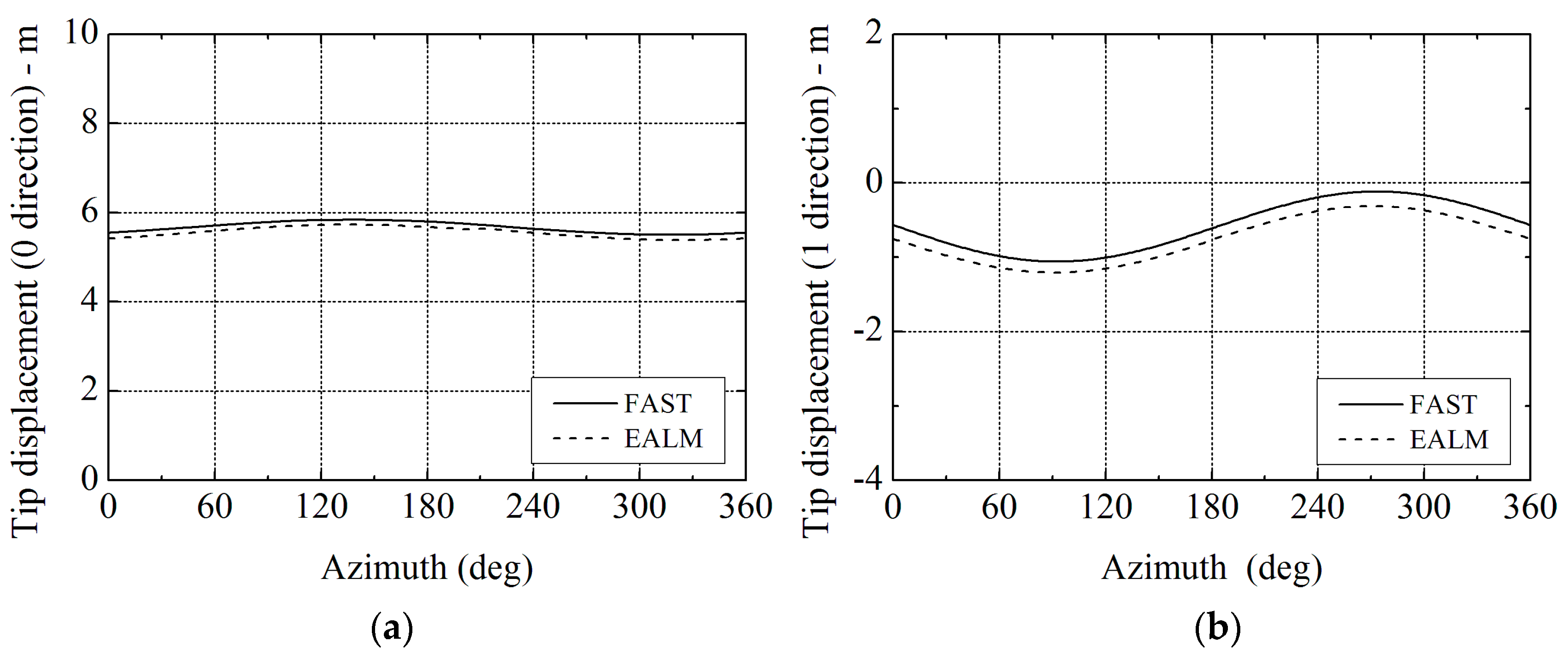
From the Figure 15, the results agree well with each other. Moreover, it can be seen that all the Pearson correlation coefficients are not less than 99% from

Table 10. Comparison of blade tip displacement Pearson simplified correlation coefficient between elastic actuator line model (EALM) and NREL’s FAST code.

Wind Speed (m/s)	Direction	R
8.0	0	99.18%
	1	99.91%
11.4	0	99.40%
	1	99.97%

, which means the curves of two methods have strong relativity. Consequently, it could be concluded that EALM can calculate reliable structural responses.

4. Aeroelastic Performance Analysis

4.1. Influence on Aerodynamic Performance

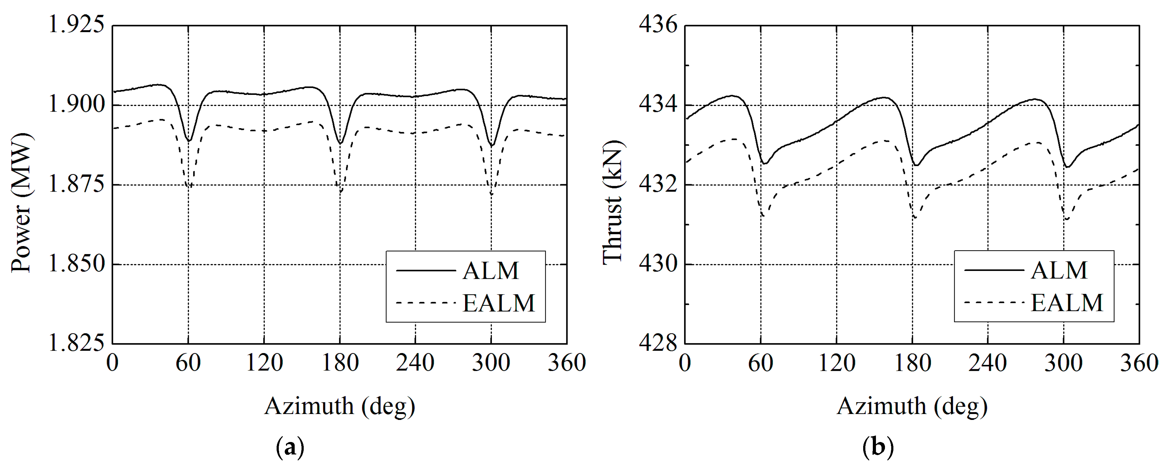
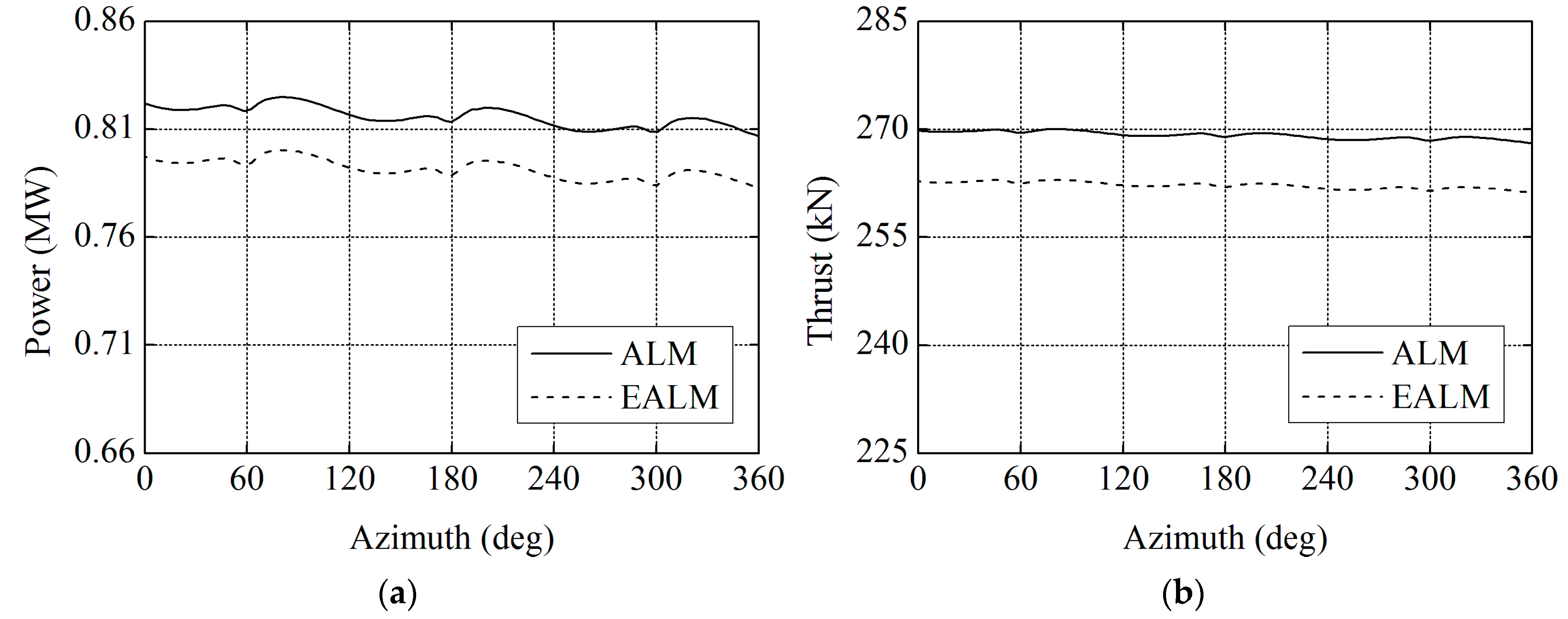
This section will discuss the influence of elastic blade on the aerodynamic performance. Figure 17 and Figure 18 depict the power and thrust azimuthal history with traditional actuator line model (ALM) and elastic actuator line model (EALM) at 8 m/s and 11.4 m/s. The ALM results are achieved by hiding the part of rotating beam solver in EALM, and the parameters setting are all the same. The curves fluctuate every 60 degrees, which is caused by the tower shadow effect. When the structural deformation is considered, the mean power reduces about 11.38 kW in 8 m/s and 11.43 kW in 11.4 m/s. Besides, the averaged thrust decreases approximately 1.08 kN in 8 m/s and 0.35 kN in 11.4 m/s. It indicates that the influence of elasticity on mean power and thrust is small in the rated condition. As the blade passes through tower, the reduction of output power turns into 15.33 kW in 8 m/s and 31.45 kW in 11.4 m/s. The decrement of thrust changes into 1.32 kN in 8 m/s and 0.96 kN in 11.4 m/s. The distance between tower and blade gets closer due to the blade deformation. Hence, the tower shadow effect becomes more serious and the decrement of power and thrust is larger. Because the blade displacement in high wind speed is large, the tower effect is the most serious in the rated wind speed and its reduction is more than that in 8 m/s.

The stabilization of the normal and tangential force is present by standard deviation, as shown in Figure 19. The standard deviation s is defined as follows:

$$s=\sqrt{s^2}=\sqrt{\frac{{\displaystyle \sum _{i=1}^n{(x_i-\overline{x})}^2}}{n-1}}$$

(36)

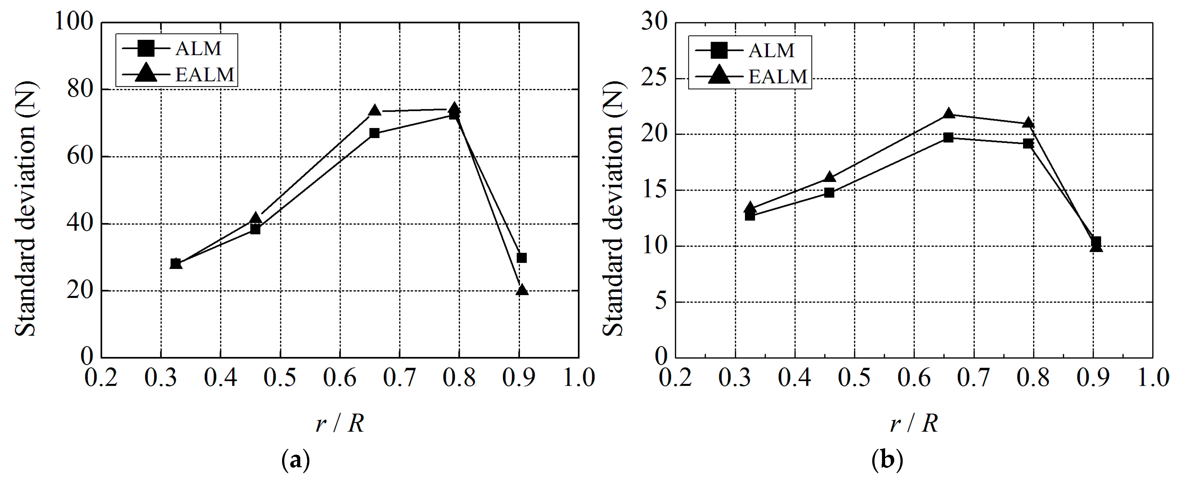
where n is sample size; $x_i$ is the individual sample points indexed with I; and $\overline{x}$ is expectation, which is the mean value of sample. From the figure, the standard deviation of the loads on blade increases a little when the elasticity of the blades is considered.

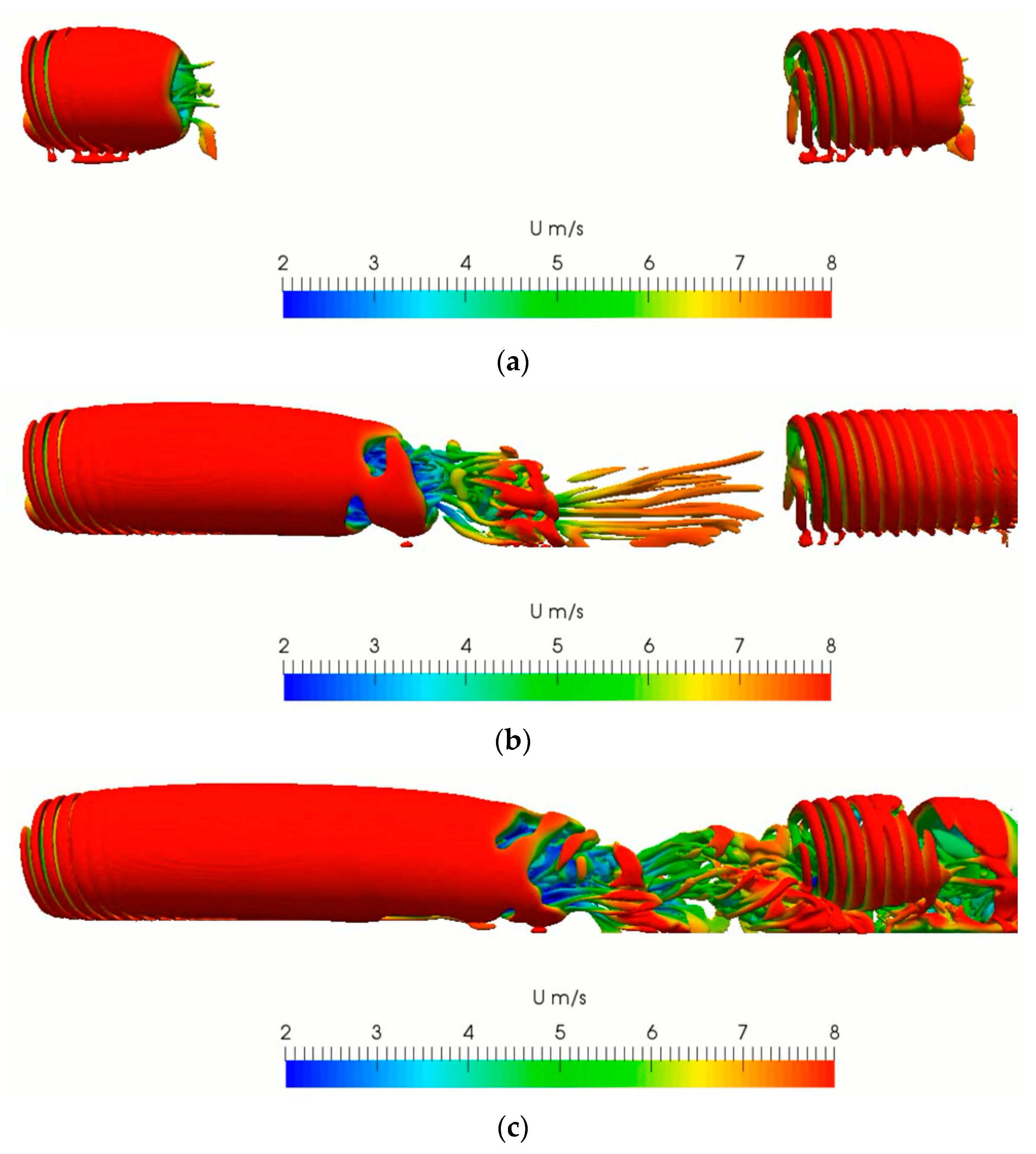
Figure 20 shows the wake structure comparison with EALM and ALM at 8 m/s. The wake vorticities are described by Q criterion, in which Q is calculated by the second invariant of the velocity gradient tensor and are stained by velocity field. The tip and hub vorticities are clear to be seen behind the rotor. The velocity in the internal surface of vorticities is smaller than the outside one. That is because the wind turbine extract momentum from the incoming airflow passing through it, and the wind energy is turned into mechanical energy, which causes the wind velocity after the rotor decreased.

The blade deflection is abbreviated and described in Figure 21. The deformation is too small to be discovered in 1 direction from left side view. Besides, it focuses on blade tip in 0 direction from front and vertical side view.

4.2. Wake Flows Analysis

To analyze the influence of elastic blade in the wake flows, an array of two NREL 5 MW wind turbines is studied (see Figure 7) with EALM. The results are extracted after the upstream wind turbine rotating 40 revolutions, and the corresponding simulation time is around 260 s. According to research [28], the rotor speed of downstream wind turbine is set as 8.11 rpm to maximize its output power.

The comparison of mean output power among EALM, ALM, and Jha et al. [34] is presented in

Table 11. Comparisons of mean output power with Jha et al. [34].

Research	Mean Power of Upstream Wind Turbine (MW)	Difference with Jha et al. [34]	Mean Power of Downstream Wind Turbine (MW)	Difference with Jha et al. [34]
EALM	2.0231	5.28%	0.7943	8.11%
ALM	2.0345	5.87%	0.8089	6.42%
Jha et al. [34]	1.9217	-	0.8644	-

, in which the power generated by downstream wind turbine reduces a lot and only about 40% of upstream wind turbine because of the wake flow effects. In addition, the elastic blade makes the mean power of downstream wind turbine decrease about 14.6 kW, which is bigger than 11.38 kW of upstream wind turbine. Furthermore, the power and thrust azimuthal history of downstream wind turbine are depicted in Figure 22. When the blade passes through tower, the output power reduces 24.83 kW and the thrust decreases 7.01 kN. In contrast with the reduction of 8 m/s in Section 4.1, which are 15.33 kW and 1.32 kN, respectively, the tower shadow effect becomes more serious. This phenomenon is caused by the instability of the flow filed around the blade. The velocity and turbulence intensity in the wake of upstream wind turbine are changed into unstable. In the flow field of the downstream wind turbine blade, the variety of blade deflection with time will further disturb them. That will impact the relative velocity of the blade element. Thus, it can be concluded that the decrement of power and thrust caused by elastic blade are getting larger in the wake flows according to the comparisons above.

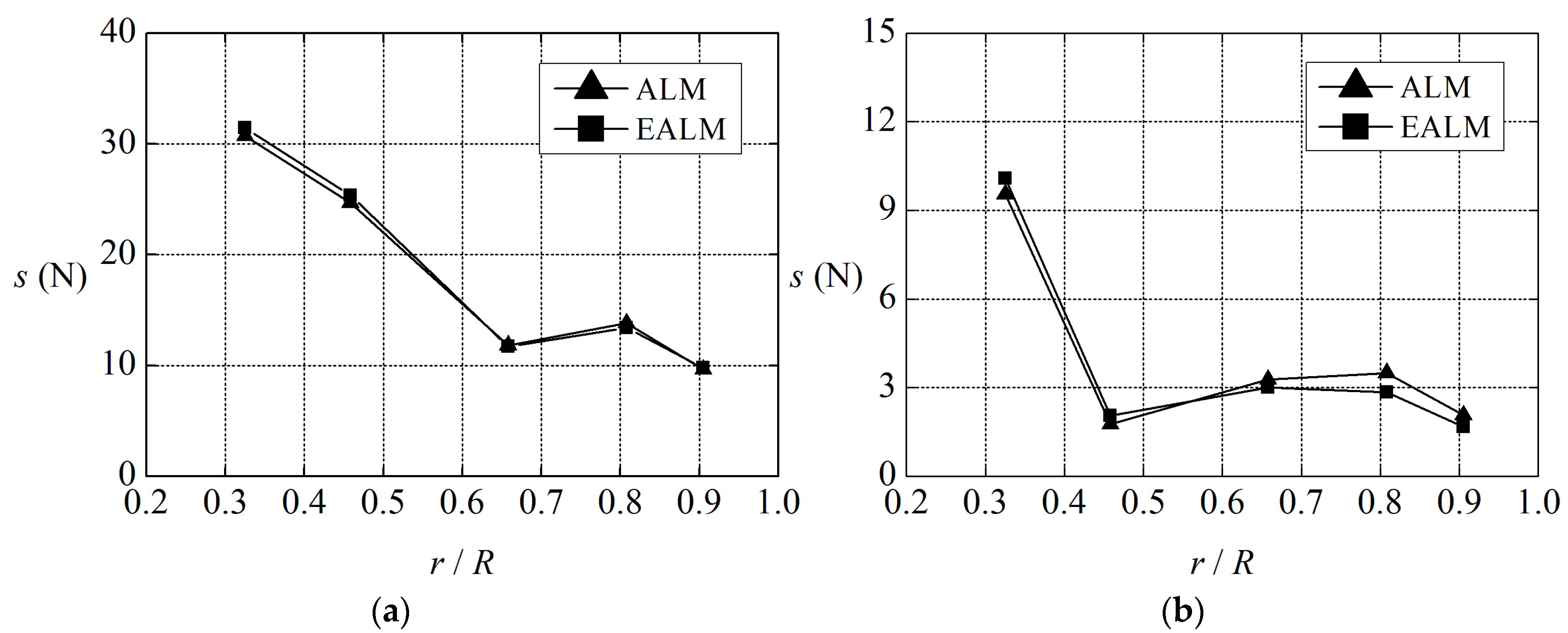
The stabilization of the normal and tangential force on downstream wind turbine blade are compared again in Figure 23. In contrast with Figure 19, the standard deviation of the loads on blade in the wake caused by upstream wind turbine getting larger when the elasticity of the blades is considered. It indicates that the influence of elastic blade becomes more serious when it is in the wake of upstream wind turbine. That will aggravate the fatigue loads and should be paid much more attention during corresponding studies.

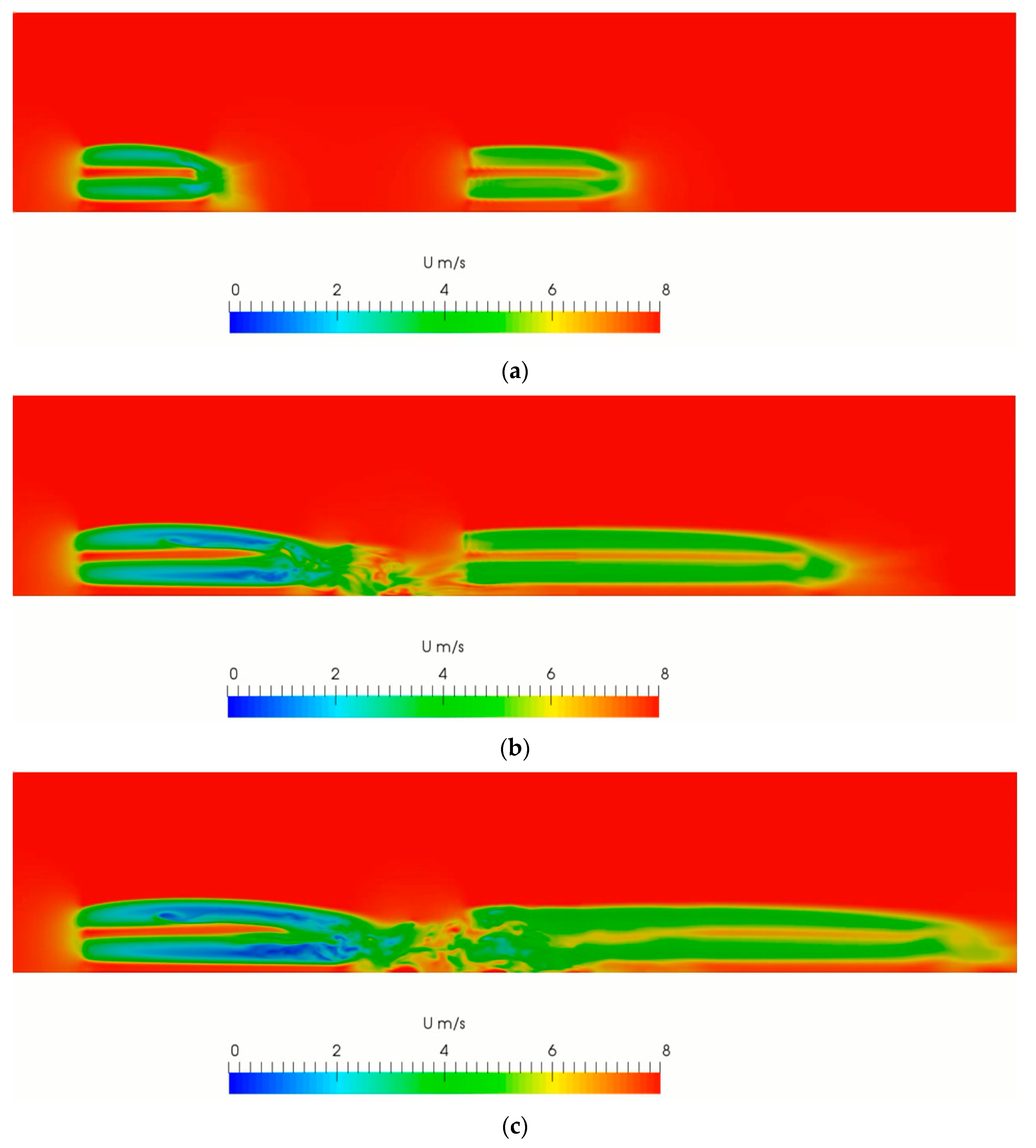
Figure 24 illustrates the process of double wind turbines array vorticity development. The wake expands as expected and the tip vorticity turns into continuum gradually in Figure 24a. Then the vorticity breakdown and the smaller-scale turbulence appears with distance increasing from upstream wind turbine (referring to Figure 24b). When the downstream wind turbine meets with this complicated wake, where the turbulence levels raise because of upstream wind turbine wakes and the momentum has not recovery completely, its tip vorticities break down earlier. That makes the wakes behind downstream wind turbine more complex, which can be seen in Figure 24c.

Figure 25 shows the development of wake velocity field correspondingly. The phenomenon of velocity deficit is easy to observe behind the rotor. Before the downstream wind turbine disturbed from the wakes generated by upstream wind turbine, the velocity field is stable relatively. As the interference status appears, the distribution of velocity field in nearby regions of downstream wind turbine is in a muddle condition. That will increase the fatigue loads on blade of downstream wind turbine.

5. Conclusions and Discussions

A new elastic actuator line model, which combines the traditional actuator line model and a beam solver used in the blade design, is proposed to study the aeroelastic performance of wind turbine efficiently. The validation is set up through comparing the result of the power, the thrust, and the tip deflection with different research. It is found that this new model can obtain acceptable prediction, including aeroelastic performance and wake fields. Besides, the tip displacement in 0 direction is the nearest with the reference data from official technical report given by NREL’s FAST code among these studies. Furthermore, the elasticity of the blades can aggravate tower shadow effect and has the possibility of wind turbine instability. The fatigue loads on the blades also become more serious. When the wake effect generated by upstream wind turbine is considered, the impact above will get more obvious.

However, this new elastic actuator line model is incomplete and needs to be improved. For example, the modal shape and natural frequency results are not yet considered. The purpose of this study is to propose an approach for investigating the aeroelastic performance rapidly. Further study is still required to refine the solver of structural dynamic characteristics and wave interactions [35].

References

- Agarwal, P.; Manuel, L. Simulation of offshore wind turbine response for long-term extreme load prediction. Eng. Struct. 2009, 31, 2236–2246. [Google Scholar] [CrossRef]
- Ghassempour, M.; Failla, G.; Arena, F. Vibration mitigation in offshore wind turbines via tuned mass damper. Eng. Struct. 2019, 183, 610–636. [Google Scholar] [CrossRef]
- Kim, D.H.; Lee, S.G.; Lee, I.K. Seismic fragility analysis of 5MWoffshore wind turbine. Renew. Energy 2014, 65, 250–256. [Google Scholar] [CrossRef]
- Santangelo, F.; Failla, G.; Santini, A.; Arena, F. Time-domain uncoupled analyses for seismic assessment of land-based wind turbines. Eng. Struct. 2016, 123, 275–299. [Google Scholar] [CrossRef]
- Rendon, E.A.; Manuel, L. Long-term loads for a monopile-supported offshore wind turbine. Wind Energy 2012, 17, 209–223. [Google Scholar] [CrossRef]
- Alati, N.; Failla, G.; Arena, F. Seismic analysis of offshore wind turbines on bottom-fixed support structures. Philos. Trans. R. Soc. A 2015, 373, 20140086. [Google Scholar] [CrossRef]
- Dong, W.; Moan, T.; Gao, Z. Long-term fatigue analysis of multi-planar tubular joints for jacket-type offshore wind turbine in time domain. Eng. Struct. 2011, 33, 2002–2014. [Google Scholar] [CrossRef]
- Jonkman, J.; Butterfield, S.; Musial, W.; Scott, G. Definition of a 5-MW Reference Wind Turbine for Offshore System Development; National Renewable Energy Laboratory technical report; National Renewable Energy Laboratory (NREL): Golden, CO, USA, 2009.
- Bak, C.; Zahle, F.; Bitshe, R.; Kim, T.; Yde, A.; Henriksen, L.C.; Natarajan, A.; Hansen, M. Description of the DTU 10 MW Reference Wind Turbine; Technical University of Denmark Wind Energy report; DTU Wind Energy: Frederiksborgvej, Denmark, 2013. [Google Scholar]
- Tran, T.T.; Ryu, G.J.; Kim, Y.H.; Kim, D.H. CFD-Based Design Load Analysis of 5MW Offshore Wind Turbine. In Proceedings of the 9th International Conference on Mathematical Problems in Engineering, Aerospace and Sciences, Vienna, Austria, 10–14 July 2012; Volume 1493, pp. 533–545. [Google Scholar]
- Miao, W.P.; Li, C.; Pavesi, G.; Yang, J.; Xie, X.Y. Investigation of wake characteristics of a yawed HAWT and its impacts on the inline downstream wind turbine using unsteady CFD. J. Wind Eng. Ind. Aerodyn. 2017, 167, 60–71. [Google Scholar] [CrossRef]
- Liu, Y.C.; Xiao, Q.; Incecik, A.; Peyrard, C.; Wan, D.C. Establishing a fully coupled CFD analysis tool for floating offshore wind turbines. Renew. Energy 2017, 112, 280–301. [Google Scholar] [CrossRef] [Green Version]
- Ma, Z.; Zeng, P.; Lei, L.P. Analysis of the coupled aeroelastic wake behavior of wind turbine. J. Fluids Struct. 2019, 84, 466–484. [Google Scholar] [CrossRef]
- Zhang, P.T.; Huang, S.H. Review of aeroelasticity for wind turbine: Current status, research focus and future perspectives. Front. Energy 2011, 5, 419–434. [Google Scholar] [CrossRef]
- Zienkiewicz, O.C.; Taylor, R.L. The finite element method. McGraw-Hill Lond. 1977, 3, 39–84. [Google Scholar]
- Ferede, E.; Abdalla, M.M.; van Bussel, G.J.W. Isogeometric based framework for aeroelastic wind turbine blade analysis. Wind Energy 2017, 20, 193–210. [Google Scholar] [CrossRef]
- Li, Y.; Castro, A.M.; Sinokrot, T.; Prescott, W.; Carrica, P.M. Coupled multi-body dynamic and CFD for wind turbine simulation explicit wind turbulence. Renew. Energy 2015, 76, 338–361. [Google Scholar] [CrossRef]
- Ageze, M.B.; Hu, Y.; Wu, H.C. Comparative Study on Uni- and Bi-Directional Fluid Structure Coupling of Wind Turbine Blades. Energies 2017, 10, 1499. [Google Scholar] [CrossRef] [Green Version]
- Heinz, J.C.; Sørensen, N.N.; Zahle, F. Fluid-structure interaction computations for geometrically resolved rotor simulations using cfd. Wind Energy 2016, 19, 2205–2221. [Google Scholar] [CrossRef]
- Sørensen, J.N.; Shen, W.Z. Numerical modeling of wind turbine wakes. J. Fluids Eng. 2002, 124, 393–399. [Google Scholar] [CrossRef]
- Fleming, P.; Gebraad, M.O.; Lee, S.; van Wingerden, J.W.; Johnson, K.; Churchfield, M.; Michalakes, J.; Spalart, P.; Moriarty, P. Simulation comparison of wake mitigation control strategies for a two-turbine case. Wind Energy 2015, 18, 2135–2143. [Google Scholar] [CrossRef]
- Na, J.S.; Koo, E.; Munoz-Esparza, D.; Jin, E.K.; Linn, R.; Lee, J.S. Turbulent kinetics of a large wind farm and their impact in the neutral boundary layer. Energy 2016, 95, 79–80. [Google Scholar] [CrossRef] [Green Version]
- Meng, H.; Lien, F.-S.; Li, L. Elastic actuator line modelling for wake-induced fatigue analysis of horizontal axis wind turbine blade. Renew. Energy 2018, 116, 423–437. [Google Scholar] [CrossRef]
- Hansen, M.O.L. Aerodynamics of Wind Turbines; Earthscan: London, UK; Sterling, AV, USA, 2008. [Google Scholar]
- TurbinesFoam. 2014. Available online: https://github.com/turbinesFoam (accessed on 16 January 2019).
- Shives, M.; Crawford, C. Mesh and load distribution requirement for actuator line CFD simulations. Wind Energy 2013, 16, 1183–1196. [Google Scholar] [CrossRef]
- Shen, W.Z.; Mikkelsen, R.; Sørensen, J.N. Tip Loss Corrections for Wind Turbine Computations. Wind Energy 2005, 8, 457–475. [Google Scholar] [CrossRef]
- Yu, Z.Y.; Zheng, X.; Ma, Q.W. Study on Actuator Line Modeling of Two NREL 5-MW Wind Turbine Wakes. Appl. Sci. 2018, 8, 434. [Google Scholar] [CrossRef] [Green Version]
- Ferziger, J.H.; Peric, M. Computational Methods for Fluid Dynamics; Springer Science & Business: Berlin, Germany, 2012. [Google Scholar]
- Jeong, M.; Cha, M.; Kim, S.; Lee, L. Numerical investigation of optimal yaw misalignment and collective pitch angle for load imbalance reduction of rigid and flexible hawt blades under sheared wind inflow. Energy 2015, 84, 518–532. [Google Scholar] [CrossRef]
- Ponta, F.L.; Otero, A.D.; Lago, L.I.; Rajan, A. Effect of rotor deformation in wind-turbine performance: Dynamic rotor deformation blade element momentum model (DRD-BEM). Renew. Energy 2016, 92, 157–170. [Google Scholar] [CrossRef] [Green Version]
- Yu, D.O.; Kwon, O.J. A coupled CFD-CSD method for predicting HAWT rotor blade performance. In Proceedings of the 51st AIAA Aerospace Science Meeting Including the New Horizons Forum and Aerospace Exposition, Grapevine, TX, USA, 7–10 January 2013; p. 911. [Google Scholar]
- Yu, D.O.; Kwon, O.J. Time-accurate aeroelastic simulations of a wind turbine in yaw and shear using a coupled CFD-CSD method. In Proceedings of the Science of Making Torque from Wind 2014 (TORQUE 2014), Copenhagen, Denmark, 18–20 June 2014; p. 524. [Google Scholar]
- Choi, N.J.; Nam, S.H.; Jeong, J.H.; Kim, K.C. Numerical study on the horizontal axis turbines arrangement in a wind farm: Effect of separation distance on the turbine aerodynamic power output. J. Wind Eng. Ind. Aerodyn. 2013, 117, 11–17. [Google Scholar] [CrossRef]
- Zheng, X.; Shao, S.D.; Khayyer, A.; Duan, W.Y.; Ma, Q.W.; Liao, K.P. Corrected first-order derivative ISPH in water wave simulations. Coast. Eng. Res. 2017, 59, 1750010. [Google Scholar] [CrossRef]
Figure 1.
Blades represented by actuator line and discretized into actuator sections.
Figure 2.
Coordinate system of the blade deflection.
Figure 3.
The diagrammatic sketch of the forces on the cantilever beam.
Figure 4.
The blade element in the local coordinate system.
Figure 5.
The computational flow chart of new elastic actuator line model.
Figure 6.
The simulation domain of single wind turbine.
Figure 7.
The simulation domain of double wind turbines.
Figure 8.
Relationship between actuator point number and aerodynamic coefficient, (a) power coefficient, and (b) thrust coefficient.
Figure 9.
Comparison of different cases results in 8 m/s: (a) power; and (b) thrust Case 1: Elastic Actuator Line Model (present study); Case 2: NREL’s FAST code; Case 3: Horizontal Axis Wind turbine simulation Code 2nd generation results; Case 4: research by Li et al. [17]; Case 5: research by Jeong et al. [30]; Case 6: research by Ponta et al. [31]; Case 7: research by Yu et al. [32,33]; Case 8: research by Ma et al. [13].
Figure 10.
Comparison of different cases results in 11.4 m/s: (a) power; and (b) thrust Case 1: Elastic Actuator Line Model (present study); Case 2: NREL’s FAST code; Case 3: Horizontal Axis Wind turbine simulation Code 2nd generation results; Case4: research by Li et al. [17]; Case 5: research by Jeong et al. [30]; Case 6: research by Ponta et al. [31]; Case 7: research by Yu et al. [32,33]; Case 8: research by Ma et al. [13].
Figure 11.
Comparisons of the aerodynamic performance results between elastic actuator line model (EALM) and NREL’s FAST code at different wind speeds: (a) thrust; and (b) power.
Figure 12.
Comparison of different cases tip displacement results in 8 m/s: (a) 0 direction; and (b) 1 direction Case 1: Elastic Actuator Line Model (present study); Case 2: NREL’s FAST code; Case 3: research by Li et al. [17]; Case 4: research by Yu et al. [32,33]; Case 5: research by Ma et al. [13].
Figure 13.
Comparison of different tip displacement results in 11.4 m/s: (a) 0 direction; and (b) 1 direction Case 1: Elastic Actuator Line Model (present study); Case 2: NREL’s FAST code; Case 3: research by Li et al. [17]; Case 4: research by Yu et al. [32,33]; Case 5: research by Ma et al. [13].
Figure 14.
Comparison of the tip displacement results between elastic actuator line model (EALM) and NREL’s FAST code at different wind speeds: (a) in 0 direction; and (b) in 1 direction.
Figure 15.
Comparison of azimuthal variations of blade tip deformations between elastic actuator line model (EALM) and NREL’s FAST code at 8 m/s: (a) in 0 direction; and (b) in 1 direction.
Figure 16.
Comparison of azimuthal variations of blade tip deformations between elastic actuator line model (EALM) and NREL’s FAST code at 11.4 m/s: (a) in 0 direction; and (b) in 1 direction.
Figure 17.
Comparisons of the aerodynamic performance results between traditional actuator line model (ALM) and elastic actuator line model (EALM) at 8 m/s: (a) power; and (b) thrust.
Figure 18.
Comparisons of the aerodynamic performance results between traditional actuator line model (ALM) and elastic actuator line model (EALM) at 11.4 m/s: (a) power; and (b) thrust.
Figure 19.
Stabilization of forces on blade: (a) normal force; and (b) tangential force.
Figure 20.
The wake structures in terms of Q field at 8 m/s: (a) by EALM; and (b) by ALM.
Figure 21.
The abbreviated sketches of blade deflection: (a) front side view; (b) left side view; (c) vertical side view; and (d) southwest isometric side view.
Figure 22.
Comparison of downstream wind turbine aerodynamic performance results between Table 8. m/s: (a) power; and (b) thrust.
Figure 23.
Stabilization of forces on downstream wind turbine blades: (a) normal force; and (b) tangential force.
Figure 24.
The wake structure development of double wind turbine aligned: (a) initial status without disturb; (b) developing status; and (c) interference status.
Figure 25.
The wake velocity field development of double wind turbine aligned: (a) initial status without disturb; (b) developing status; and (c) interference status.