Article

Time-Lapse Seismic and Electrical Monitoring of the Vadose Zone during a Controlled Infiltration Experiment at the Ploemeur Hydrological Observatory, France

1
CNRS, Géosciences Rennes—UMR 6118, Université Rennes, F-35000 Rennes, France
2
CNRS, EPHE, METIS, Sorbonne Université, F-75005 Paris, France
3
Institut de physique du globe de Paris, CNRS, Université de Paris, F-75005 Paris, France
4
Institute of Earth Sciences, University of Lausanne, CH-1015 Lausanne, Switzerland
*
Author to whom correspondence should be addressed.
Water 2020, 12(5), 1230; https://doi.org/10.3390/w12051230
Submission received: 31 March 2020 / Revised: 21 April 2020 / Accepted: 21 April 2020 / Published: 25 April 2020
(This article belongs to the Special Issue Applied Geophysics in Hydrogeological Practice)

Abstract

:
The vadose zone is the main host of surface and subsurface water exchange and has important implications for ecosystems functioning, climate sciences, geotechnical engineering, and water availability issues. Geophysics provides a means for investigating the subsurface in a non-invasive way and at larger spatial scales than conventional hydrological sensors. Time-lapse hydrogeophysical applications are especially useful for monitoring flow and water content dynamics. Largely dominated by electrical and electromagnetic methods, such applications increasingly rely on seismic methods as a complementary approach to describe the structure and behavior of the vadose zone. To further explore the applicability of active seismics to retrieve quantitative information about dynamic processes in near-surface time-lapse settings, we designed a controlled water infiltration experiment at the Ploemeur Hydrological Observatory (France) during which successive periods of infiltration were followed by surface-based seismic and electrical resistivity acquisitions. Water content was monitored throughout the experiment by means of sensors at different depths to relate the derived seismic and electrical properties to water saturation changes. We observe comparable trends in the electrical and seismic responses during the experiment, highlighting the utility of the seismic method to monitor hydrological processes and unsaturated flow. Moreover, petrophysical relationships seem promising in providing quantitative results.

1. Introduction

Soil moisture plays an important role in the Earth’s water balance [1,2,3]. After precipitation, for instance, water content increases in a soil further influencing water fluxes such as groundwater recharge, surface runoff, and evapotranspiration. These processes characterize the critical zone and are closely related to ecosystems’ productivity, climate variability, slope stability, and water availability and quality [4,5], hence the interest in measuring soil moisture and mapping its temporally varying distribution in the subsurface.
The vadose zone, also termed the unsaturated zone, is governed by strong spatiotemporal variability posing important challenges for hydrological characterization [6]. Classical soil moisture measuring techniques are intrusive (i.e., they are based on analyzing soil samples in the laboratory), and more modern techniques such as Time Domain Reflectometry (TDR) or Frequency Domain Reflectometry (FDR), while non-intrusive and adapted to in situ conditions, are still limited in terms of coverage and the small support volume of measurements [7].
To overcome these limitations, hydrogeologists have increasingly turned to geophysical methods over the past three decades [8,9]. The combined use of multiscale probing and imaging techniques along with the integration of hydrological, hydrogeological, and hydrogeochemical data is now commonplace for the observation and study of the surface–subsurface continuum [10]. This approach, often referred to as hydrogeophysics, can be applied non-intrusively from the surface to provide information about subsurface properties related to hydrogeological structures at appropriate scales. Moreover, time-lapse geophysical applications have proven useful for monitoring flow and water content dynamics [11].
In vadose zone hydrogeophysics, electrical and electromagnetic methods dominate due to the clear links between the physical properties they sense and water content. Being mainly dependent on mechanical properties, seismic prospecting techniques are commonly used at larger scales and for other application areas [10]. The seismic signal is by definition related to elastic wave propagation velocities that in turn depend on the material’s mineral composition, porosity, state of stress, and degree of saturation. Seismic imaging has been classically used to characterize geological structures [12,13,14], yet seismic responses are also influenced by hydrological properties and state variables [15], a recognition that has led to evermore studies using seismic data to constrain hydrological models.
Pressure (P) and shear (S) wave velocities (VP and VS) can be estimated from various seismic techniques [16,17]. P- and S-waves are affected differently by changes in pore fluid saturation and their ratio (VP/VS) permits imaging fluids in rocks. For applications to characterize the critical zone, it is possible to combine P- and S-wave refraction tomography [18,19] or to use surface-wave profiling methods [20,21]. These approaches have been tested in further studies [22,23] and applied for quantitative estimations of hydrological parameters in hydrothermal contexts [24]. Nevertheless, there are inherent incompatibilities between P-wave tomography and surface-wave analysis as they involve distinct wavefield examinations and different assumptions about the medium and, as a result, VP and VS models have contrasting resolutions, investigation depths, and posterior uncertainties. Moreover, the inversion processes generally use a small number of layers that cannot fully describe the continuous variations of the subsurface hydrological properties, and the spatial variability of dry properties in soils can be of greater influence in seismic wave velocities than the variation of water content itself. Consequently, VP and VS models should be interpreted separately [25,26] before deriving any parameter of interest which can, in turn, lead to bias and impair monitoring applications.
These challenges propel the revision of forward models and inversion approaches, promoting an advance from structural and static property imaging to process-based imaging in order to find alternative ways to detect spatiotemporal changes in water distribution. It is important to consider the hydrological information contained in the seismic data before inverting them [27,28,29] and also to quantify their temporal variability [26] to properly understand hydrosystems dynamics.
In parallel, efforts have been made to establish physical links between seismic methods and the hydrodynamic parameters of interest, spanning theoretical and experimental approaches [30,31,32,33,34] together with field case studies [24,35] and empirical petrophysical models [36,37,38]. Nevertheless, the interpretation of the near-surface mechanical properties and the definition of their quantitative links with hydrodynamic parameters remains complex. The typical theoretical framework for studying connections between a rock’s hydrodynamic parameters and seismic properties is poroelasticity. However, most sites of interest in critical zone observatories and associated hydrosystems do not only involve consolidated rocks but also—and almost systematically—unconsolidated and partially saturated soils. In this context, the use of Effective Medium Theory (EMT) approaches (e.g., [39,40]) remains delicate as they can fail to quantitatively describe velocity profiles [41].
The use of multi-method geophysics can help overcome these limitations by decreasing ambiguities inherent to each method [42]. Regarding electrical resistivity tomography (ERT) and seismic methods, previous studies have shown correlatable trends between electrical resistivity, ρ, and P-wave seismic velocity in near-surface materials (e.g., [43,44]) while others have used both methods in time-lapse settings to study ground ice degradation [45], and infiltration and dissolution processes [46].
To further investigate the electrical and seismic response in a near-surface time-lapse setting, we designed a controlled field experiment in a critical zone observatory, in Brittany, France. We infiltrated water into a defined area using overall regular injection intervals during two days with buried TDR sensors providing real-time water content data with depth. Each infiltration event was followed by geophysical acquisitions along two superficial orthogonal lines crossing in the middle of the infiltration area. Herein, we show not only the relative changes in ρ and VP but also their evolution with water saturation and derived infiltration patterns. We explore correlations between the two geophysical properties and evaluate the agreement between the data and well-established petrophysical relationships. We discuss our results in the context of advancing the usage and interpretation of seismic data and multi-method geophysics at the near-surface field scale for hydrological applications.

2. Materials and Methods

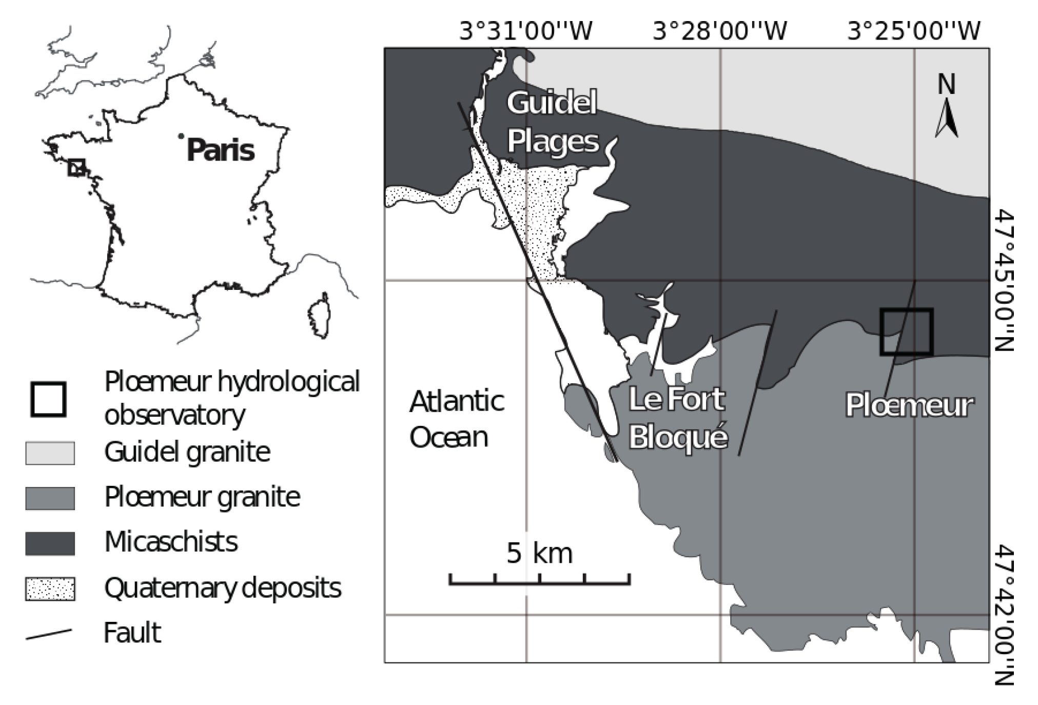
2.1. Site Description

The Ploemeur Hydrological Observatory is located in northwest France, on the south coast of Brittany, 3 km from the Atlantic Ocean (Figure 1). The crystalline bedrock aquifer in the area is composed of tectonic units developed during the Hercynian orogeny and marked by numerous synkinematic intrusions of Upper Carboniferous leucogranites [47]. A pumping site is located at the intersection of (i) a contact between the Ploemeur granite and overlying mica schists dipping 30° to the North and (ii) a sub-vertical fault zone striking N 20° [48].
Since 1991, the crystalline bedrock aquifer has annually supplied 1 million m3 of drinking water to a nearby population of 20,000 inhabitants. The well-developed and highly connected fracture network at depth makes this aquifer highly productive compared to other bedrock aquifers in Brittany. Over time, it has been developed into a well-monitored site with dense piezometric coverage involving 50 boreholes ranging from 30 to 150 m depth [49]. The mean annual precipitation and potential evapotranspiration at the site are around 900 and 600 mm/year, respectively [50], suggesting the maximum infiltration is as large as 300 mm/year, i.e., 30% of annual rainfall.
We carried out an infiltration experiment consisting of successive pulses in the micaschist area near the pumping site. In 2012, a team of researchers and students [51] dug a pit and installed sensors at different depths including thermometers, tensiometers, and TDR sensors, the latter providing real-time water content estimates throughout our experiment. They also characterized the recovered soils from the pit in terms of textural classes, type of soil, bulk density, ρb, and porosity, ϕ, as summarized in Table 1. A cross-section picture and schematic of the pit wall are shown in Figure 2. Once the sensors were installed, the pit was refilled with the same extracted soil.

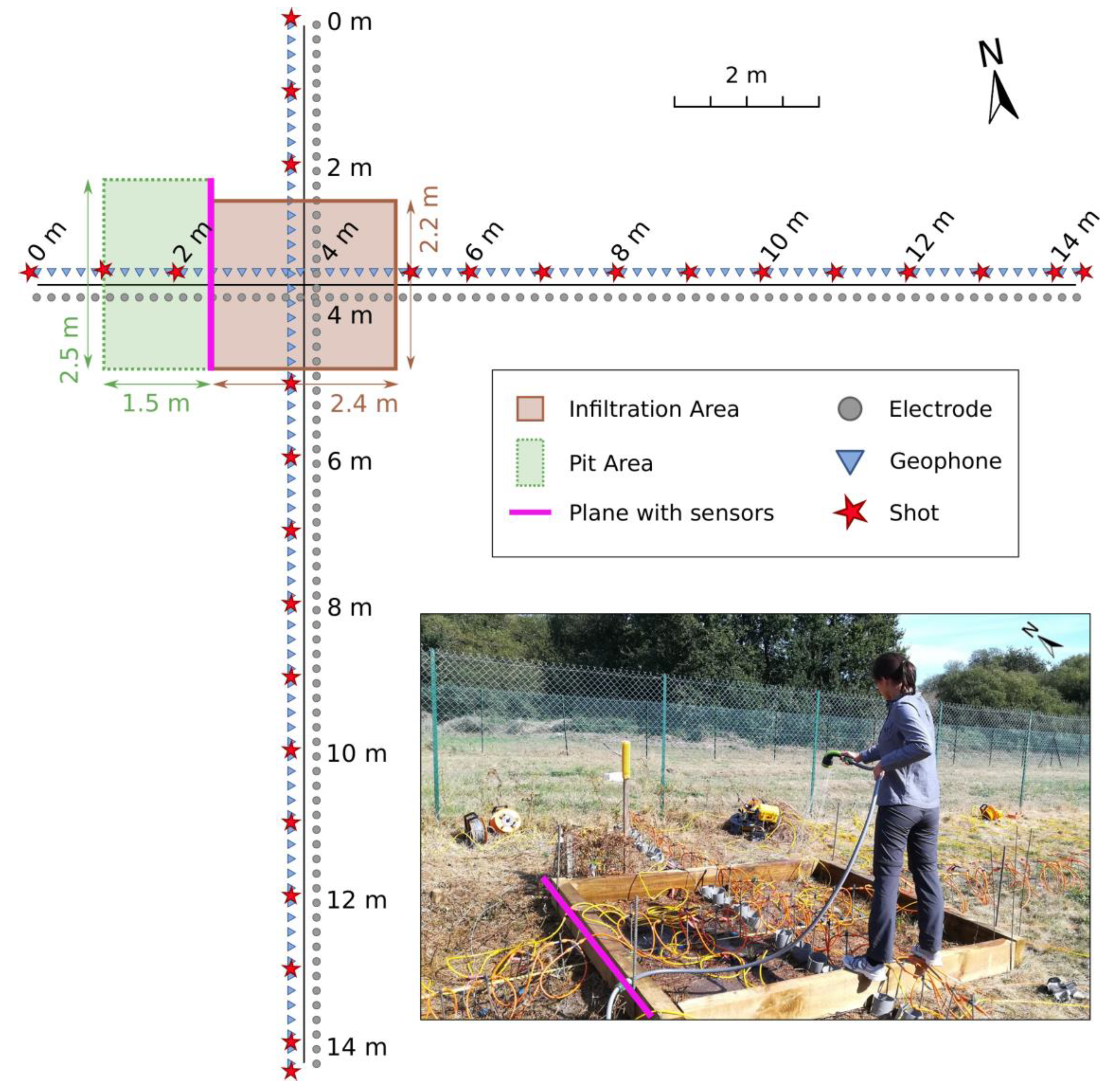
2.2. Acquisition Setup

The infiltration experiment was carried out in September 2018. We first delimited a 2.2 × 2.4 m2 rectangular area for the infiltration using wooden planks, the western side of it being adjacent to the side of the pit with the sensors. We then installed electrodes and 14-Hz vertical component geophones along two orthogonal lines, named NS and WE, crossing in the middle of the infiltration area. For the two geophysical methods, the dimensions were the same with each line being 14.2 m long with 72 sensors spaced by 20 cm.
For the ERT acquisition, we used a Wenner–Schlumberger array with 2006 quadripole configurations. As for the seismic acquisition, given the small geophone spacing and spread, the seismic source consisted of a small metallic-headed sledgehammer hit by another 2-kg sledgehammer. A total of 14 shots were made along each line with a spacing of 1 m starting at −0.1 m (i.e., 10 cm before the first geophone) and ending at 14.3 m with the spacing between the last and second last shot being 40 cm. There were no shots inside the infiltration area. At each shot position, we hit four times to increase the signal-to-noise ratio. The sampling rate was 0.125 ms, and the recording time was 800 ms. A delay of −50 ms was kept before the beginning of each record to prevent early triggering issues.
To investigate the changes in geophysical data and properties with varying water content, we adopted a time-lapse approach during two measurement days in which the responses to successive infiltrations were targeted. The first acquisition on day 1 was carried out before any forced infiltration had been made and it is referred to as the background acquisition. Each subsequent acquisition was made after an infiltration event except for the first acquisition of day 2, which was done before resuming the infiltration events. In total, we infiltrated 9 times (4 times on day 1 and 5 on day 2), and we acquired geophysical data at 11 individual acquisition times (5 times on day 1 and 6 on day 2).
The infiltrated water was pumped from a neighboring borehole. Pumping rates were continuously measured, as well as pumped water conductivity and temperature. Since the water level at the site is at 15.8 m depth, we do not expect the pumping to have affected the vadose zone dynamics or the geophysical data. We used a hose with a showerhead attached and an operator stood along the wooden planks while infiltrating (see Figure 3). To ensure uniform coverage inside the infiltration area, we steadily moved the hose during each infiltration; no standing water surface was created indicating that the injection rate was lower than the infiltration capacity of the soil (approximately 18 mm/h, measured during several tests using the Porchet method). The first two infiltration volumes were 250 liters each (approximately 45 mm), and it took 20 minutes to complete each infiltration. For the subsequent infiltrations, we used 400 liters each (approximately 75 mm) taking 35 minutes to complete each infiltration. The sensors in the subsurface continuously recorded the volumetric water content, θ, matric water potential, Ψm, and temperature, T, throughout the experiment as shown in Figure 4.
There was no rainfall during the experiment and the air temperature varied between 7 and 23 °C. The potential evapotranspiration was 3.3 mm/day, considered negligible compared to the infiltration volumes. The experiment data are openly available, information on where and how to access them is provided in Availability of Data and Materials.

3. Results

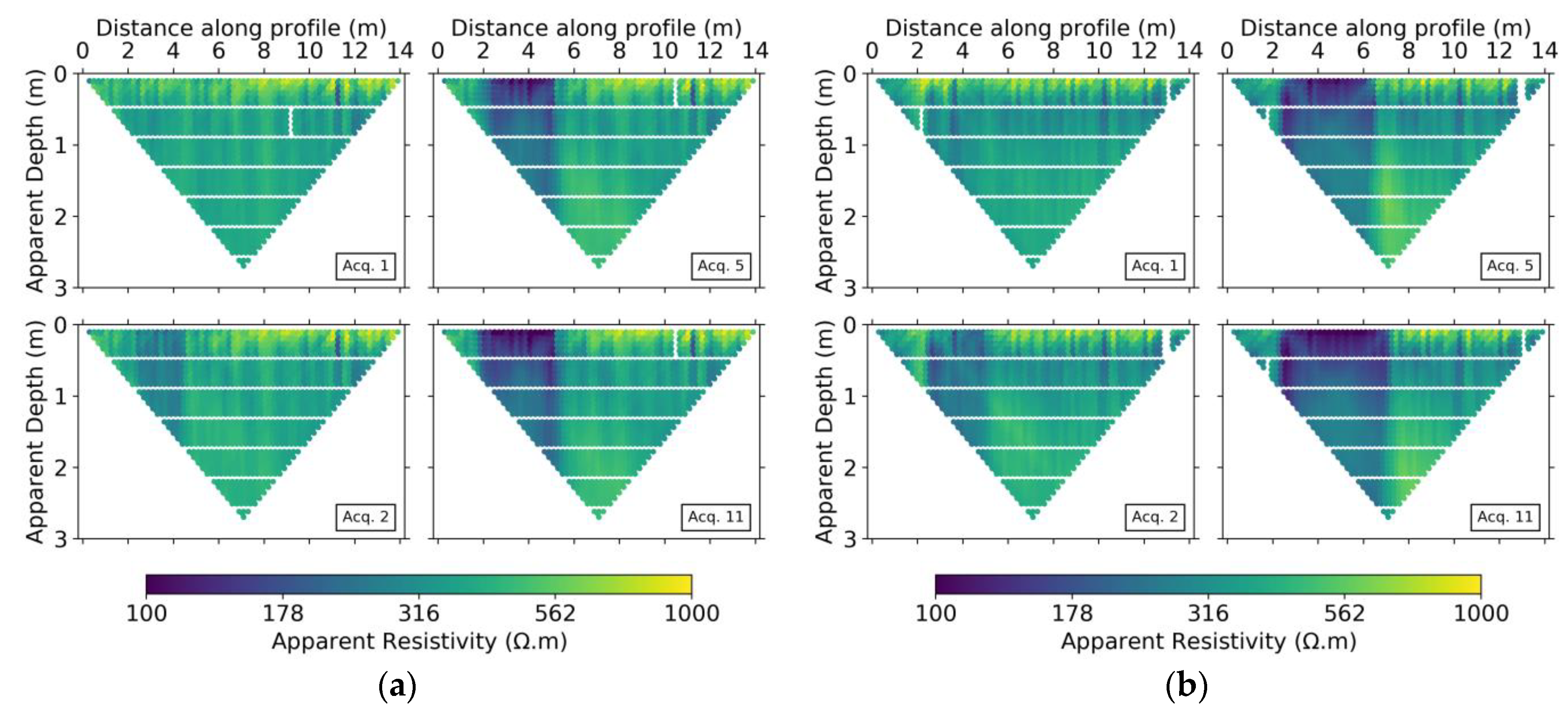
3.1. Electrical Resistivity Tomography

Before inverting the raw data, we eliminated unrealistic data points such as zero values of apparent resistivity, ρa. Figure 5 shows pseudo-sections for some of the acquisitions for both lines. As we worked with time-lapse data, the electrode configurations with bad data points during one acquisition were removed from all the others such that all acquisitions had the same number of data points using the same electrode configurations. This pruning of the data implied that the original 2006 measurements at each acquisition were reduced to 1970 and 1956 data points for the NS and WE lines, respectively, before being used for inversion.
To invert the ERT data we used the pyGIMLi library [52]. We first inverted the background acquisitions for the NS and WE lines separately. To do so, we used a homogeneous starting and reference model of 50 Ω.m. The anisotropic regularization (relative weight penalizing roughness) was set to 0.5 to favor horizontal layering and the relative error was set to 4.5% according to the largest standard deviation in the recorded data. The regularization parameter λ was initially set to 500 and decreased by 20% at each iteration until convergence. As the infiltration area only covered a segment of the line and as we are interested in retrieving a strong contrast between areas of increasing water content and areas of constant water content, we used an l1-norm mimicking minimization scheme to enhance spatial transitions in the model. The data fit criteria (chi-squared misfit χ2 normalized by the number of data points being smaller than 1) was reached at the 15th and 16th iterations for the NS and the WE line, respectively. We show the results of these background inversions in Figure 6.
For the time-lapse inversions we applied the ratio inversion scheme introduced by [53]:
d n = d n d 0 f ( m 0 ) ,
where d0 and dn are the data (in this case, apparent resistivity) for the background acquisition and the nth acquisition, respectively, f(m0) is the model response for the background acquisition, and dn’ is the new data to invert. Instead of using a uniform starting model as in [53], the starting and reference model was initially set to the resulting background model (e.g., [54]). A modified inversion approach was put into place, in which we performed the time-lapse inversions twice. In the first round, we used the l1-norm minimization scheme and set the relative error to 3% and the initial lambda to 200, decreasing it by 20% at each iteration. Then, a second time-lapse inversion was performed in which the starting and reference model at each time step were defined, for each inversion parameter, as the minimum resistivity between the model obtained from the first time-lapse inversion and the background model, while keeping the other inversion parameters unchanged. We adopted this approach to decrease the prominence of positive anomalies around the infiltration area (for an alternative formulation, see [55]). Note that the second time-lapse inversion is like any other time-lapse inversion, except for the fact that the starting and reference model favors negative changes aiming at diminishing smoothness-constrained-induced false-positive artifacts surrounding the region of large decreases. If positive increases are needed to fit the data, then positive changes will still appear in the inversion results. In Figure 7, we show the time-lapse inversion results for both lines in terms of relative change with respect to the background inversion. The decrease in resistivity grows with each acquisition reaching decreases of 90%.

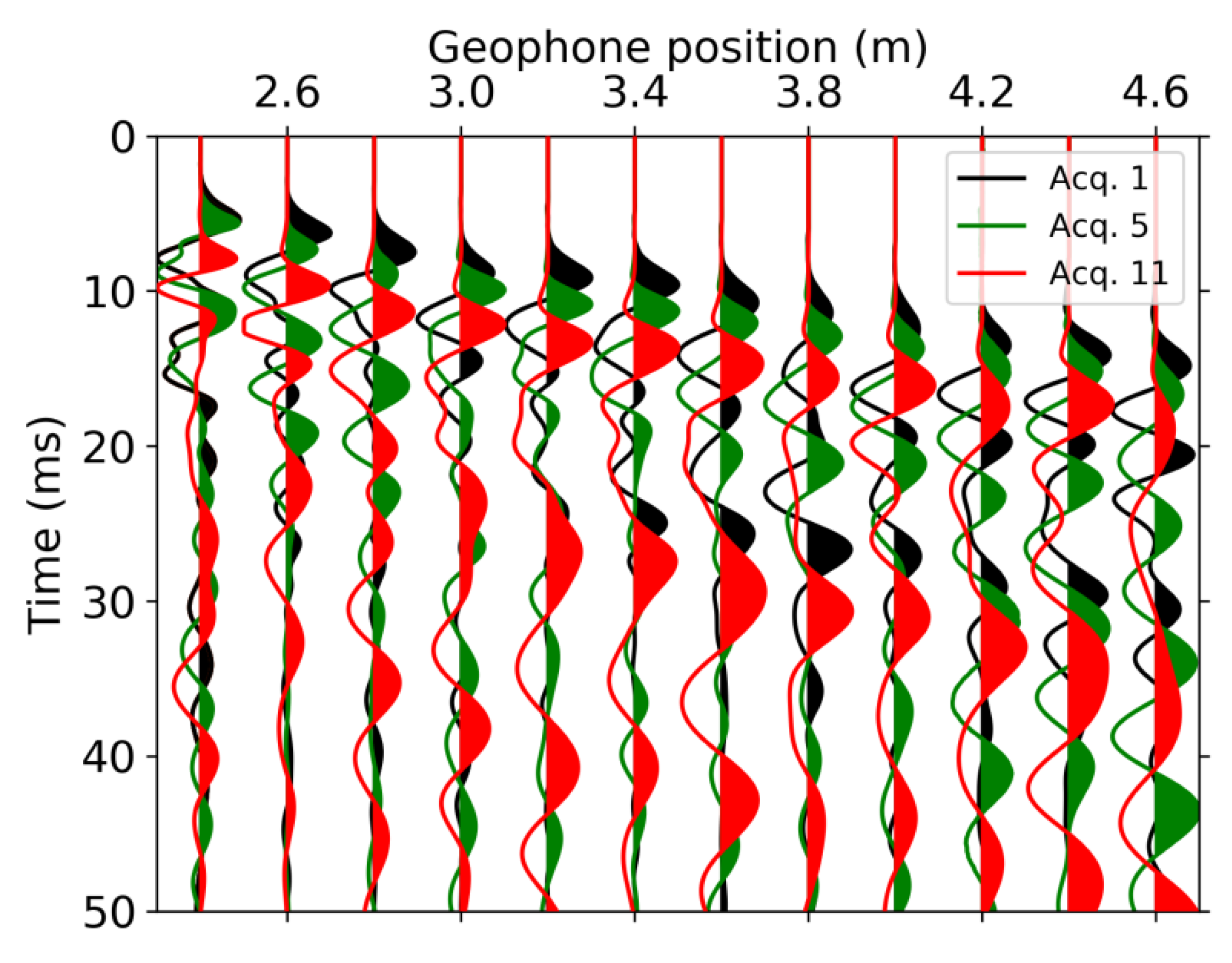
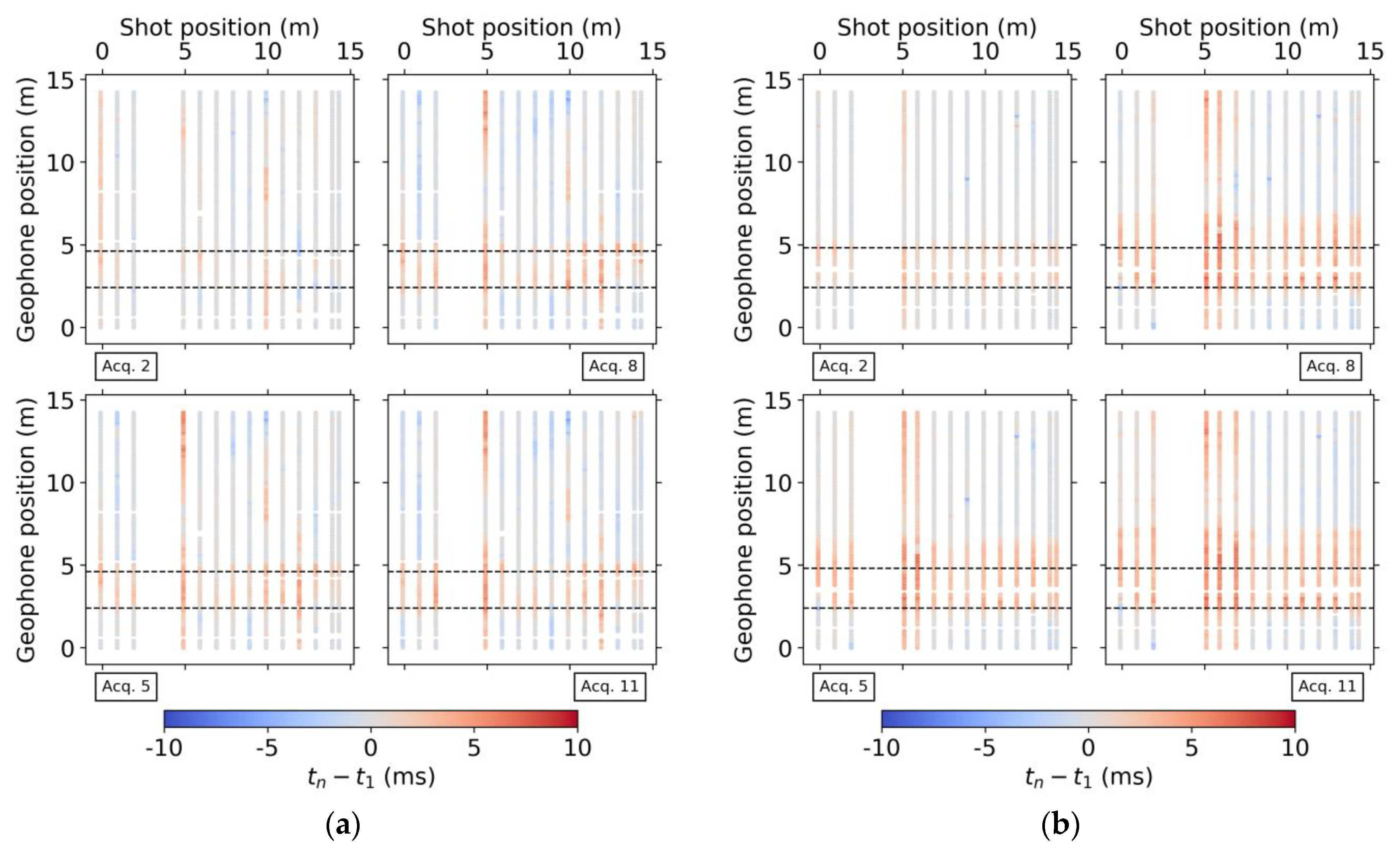
3.2. Seismic Refraction: Traveltimes and P-wave Velocity

For the seismic data, we first identified temporal changes in the seismic traces. For a given shot position, we extracted the gathers at different acquisition times and overlapped the traces; a clear shift is observed inside the infiltration area with the first arrivals of later acquisitions arriving later in time (Figure 8). To quantify these shifts, we manually picked the first-arrival traveltimes for the whole dataset. Next, we computed the differences in arrival times between each acquisition and the background acquisition. Figure 9 displays these differences for each shot-geophone pair to illustrate to which extent increases in traveltimes are due to the successive infiltration events. The increases in traveltimes sometimes extend a few meters outside the infiltration area whereas further away, the changes are minimal or slightly negative. The NS line shows more outliers in traveltime differences while the WE line has a more continuous behavior. This is likely a consequence of the noisier traces in the NS line, which made picking more difficult.
As we observed traveltime changes consistent with the infiltration, we proceeded by inverting these data to obtain a VP subsurface model using the refraction tomography module of pyGIMLi that uses Dijkstra’s algorithm [56] as the forward solver. Similarly, as for the ERT, we first inverted the background acquisitions using as starting model a gradual increase from 100 m/s at the top to 600 m/s at the bottom in accordance with expected velocity ranges in shallow soils. The reference model was the same as the starting model, and we set an absolute error of 3 ms. The regularization parameter λ was set to 200, and we applied an l1-norm scheme based on iteratively reweighted least squares both for regularization and data as we observed systematic outliers in the data (picked traveltimes). For both lines, the data were fitted in three iterations leading to the results in Figure 10.
As for the ERT, we defined a ratio correction (Equation 1) and continued with the time-lapse inversions using the same parameters as for the background inversion except for reducing the assumed absolute error to 2 ms. We tried the two-step approach as for the time-lapse ERT without significant improvement and therefore adhered to a single time-lapse inversion. Figure 11 shows the results in terms of relative change with respect to the background. We notice a clear decrease in VP inside the infiltration area, which becomes more evident at each acquisition in time, eventually reaching −60%. Outside the infiltration area, in the first one-meter depth, one can observe zones of increase in VP resulting from small decreases in traveltimes recorded at these locations.

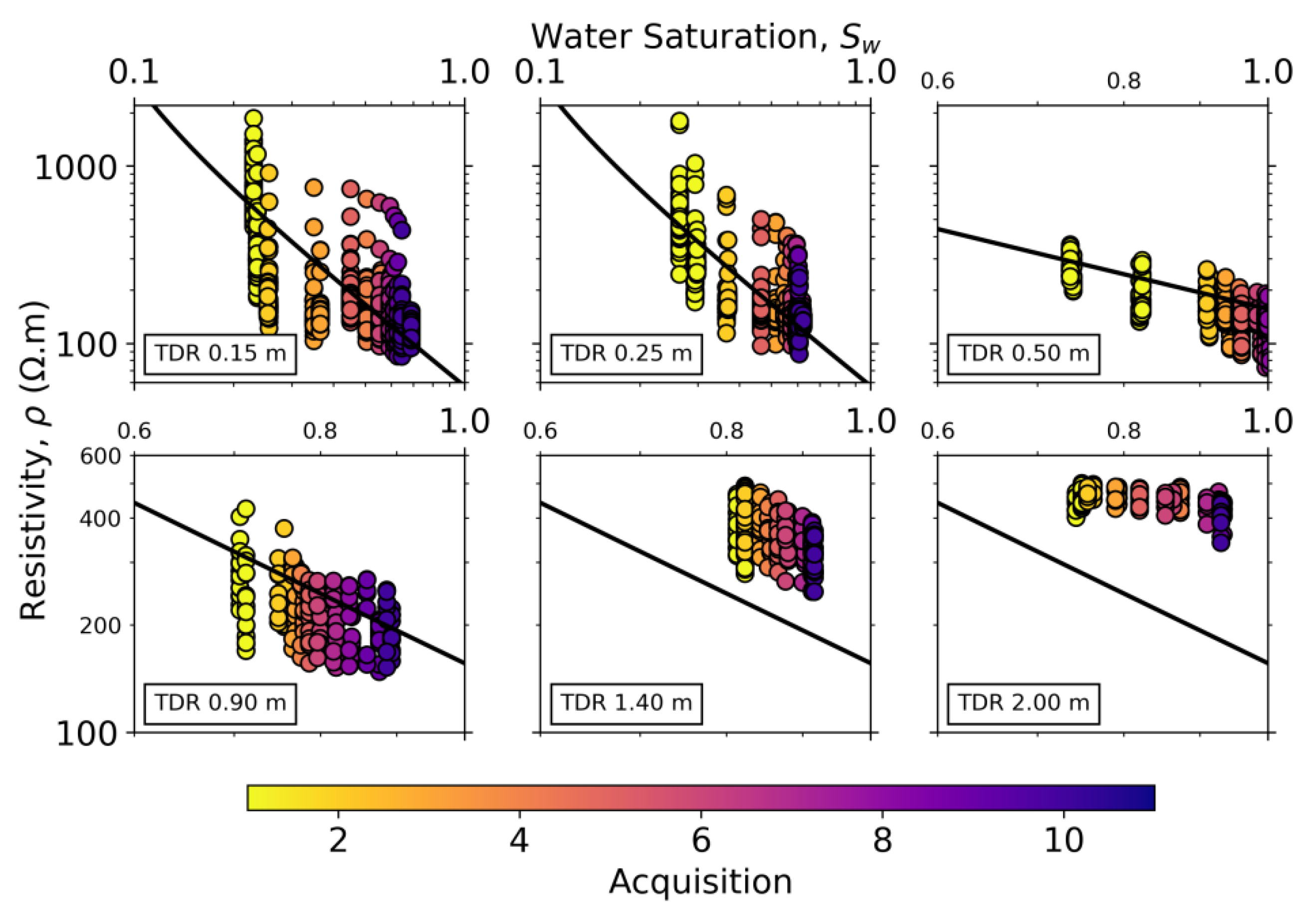
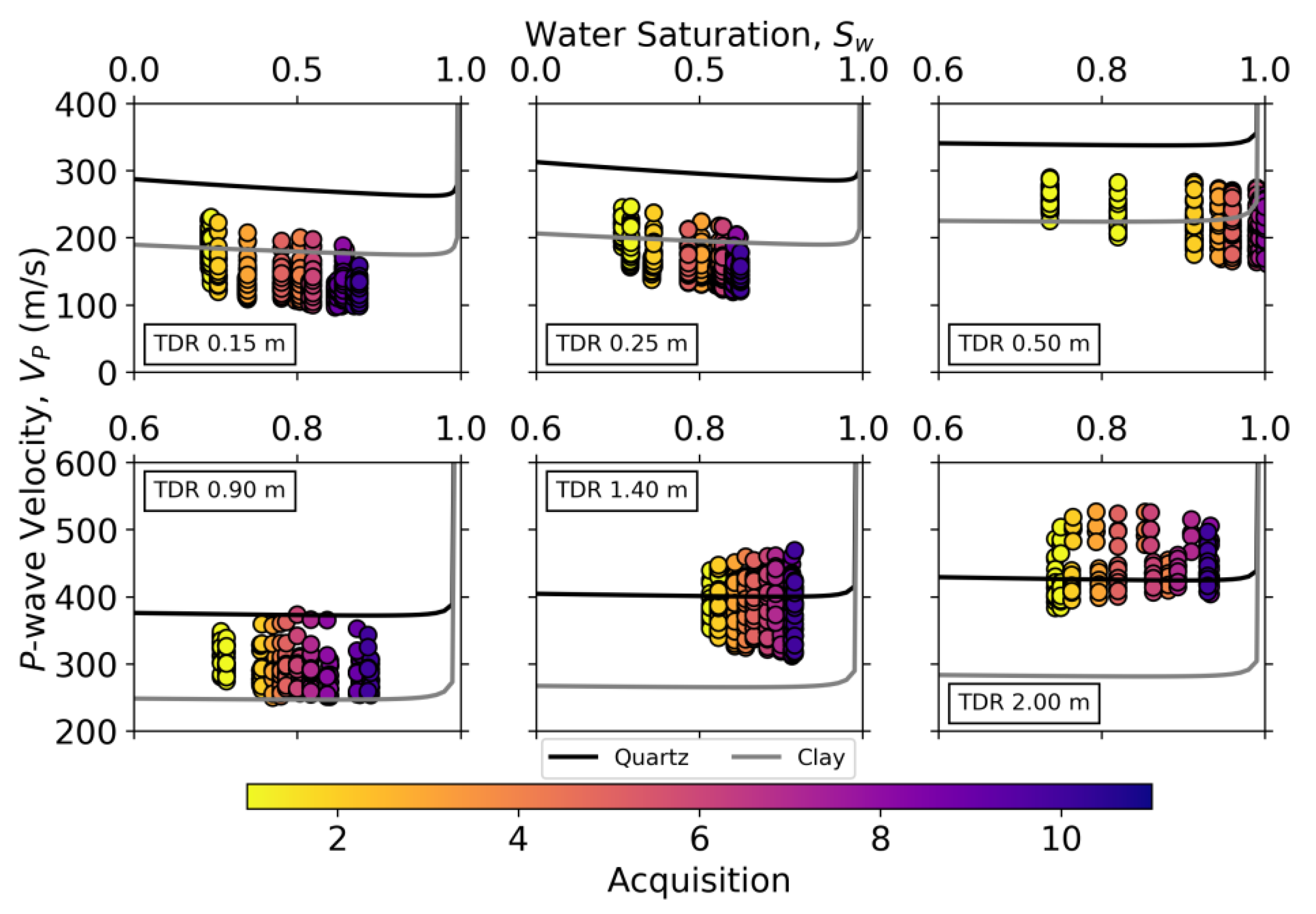
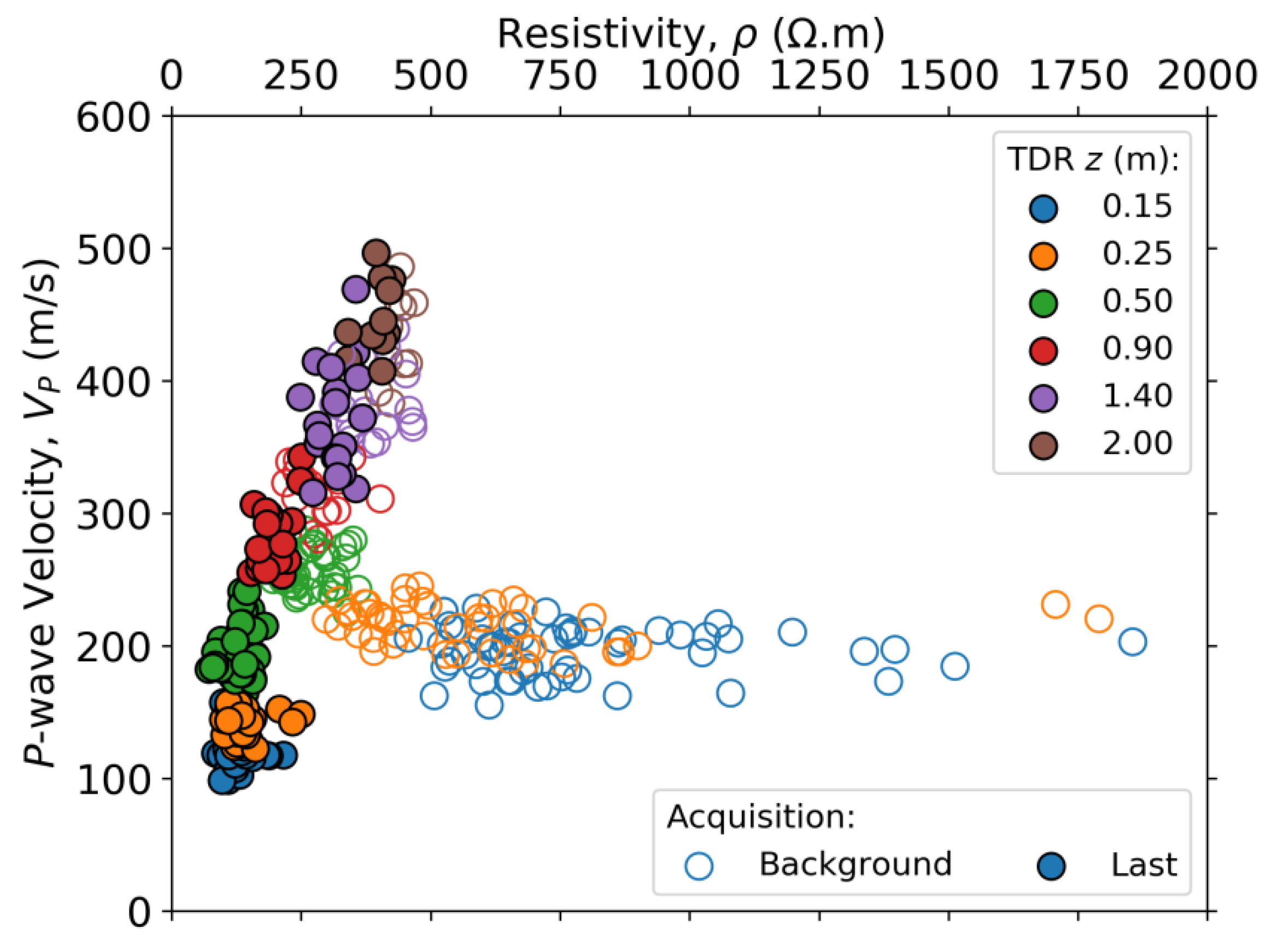
3.3. Petrophysical relationships

To further investigate the behavior of ρ and VP with varying water saturation, Sw, we extracted the resistivity and velocity values at depths corresponding to those of the subsurface sensors for all the points inside the infiltration area and all acquisitions. We converted the water content readings from the TDR sensors to Sw by means of the porosity measurements of the soil (Table 1) such that:
S w = θ ϕ ,
and plotted ρ and VP against Sw (Figure 12 and Figure 13). We compared the trends in our data with well-established models for both methods. We defined ρ as the inverse of the effective electrical conductivity, σeff, formulated by [57] as:
σ e f f = 1 F [ S w n σ w + ( F 1 ) σ s ] ,
where F = ϕ−m is the electrical formation factor, m and n are Archie’s first and second exponent [58], respectively, σw is the electrical conductivity of the pore water, and σs is the surface conduction. We compared two different models with the data, one for the two shallowest sensor positions and another one for the rest, given the different documented porosities across these depths. For the first model we used m = n = 1.5 and σs = 1 × 10⁻³ S/m, for the second one, as the porosities were lower and the soils were deeper and likely more compacted, we used m = 1.7, n = 2, and σs = 5 × 10⁻⁴ S/m. For both models we used σw = 5 × 10⁻² S/m as the mean conductivity of the pumped water measured during the experiment.
We modeled VP for two different compositions, 100% quartz and 100% clay, using an effective medium model based on Hertz–Mindlin contacts. We computed the dry effective bulk and shear moduli, Keff and µeff, for the absolutely frictionless case (formulation from [59], p. 247):
K e f f = [ C 2 ( 1 ϕ ) 2 μ 2 18 π 2 ( 1 ν ) 2 P ] 1 / 3 ,     μ e f f = 3 5 K e f f ,
where C is the average number of contacts per grain; µ and ν are the shear modulus and the Poisson ratio of the grain material, respectively; and P is the effective stress. For the 100% quartz composition we used µ = 44 GPa and ν = 0.08, and for the 100% clay composition we used µ = 9 GPa and ν = 0.34; in both cases we used C = 6. We proceeded by performing fluid substitution according to Biot–Gassmann [39,40] to obtain the saturated bulk and shear moduli, Ksat and µsat, for the whole range of 0%–100% Sw (formulation also from [59], p. 273):
K s a t K K s a t = K e f f K K e f f + K f l ϕ ( K K f l ) ,     μ s a t = μ e f f ,
where K is the bulk modulus of the grain material, and Kfl is the effective bulk modulus of pore fluid and as we deal with a partially saturated medium:
1 K f l = S w K w + 1 S w K a ,
with Kw and Ka as water and air bulk modulus, respectively (Kw = 2.2 GPa and Ka = 0.101 MPa). Together with the corresponding changes in ρb, we calculated VP as:
V P = K s a t + 4 3 μ s a t ρ b .

4. Discussion

The results obtained from ERT and seismic time-lapse inversions demonstrate the utility of geophysics in providing spatiotemporal information about hydrological processes that complement soil moisture sensors with limited spatial coverage. In Figure 14 we show the evolution of the infiltration front in the subsurface in terms of relative changes in ρ and VP. Although the choice of percentage change (−60% for ρ and −25% for VP) is rather arbitrary, one can identify large-scale similarities and smaller differences in the evolution of the two properties and between the infiltration patterns of the two lines.
Previously, cross-borehole geophysics has been successfully applied to monitor tracer infiltration (e.g., cross-borehole ERT and GPR in [60]). Herein we extend this application using surface-based ERT and seismic. From the profiles in Figure 14, we can identify preferential flow paths that are consistent for both methods, where for the NS line changes tend to evolve northwards, and for the WE line, they evolve eastwards. In the case of the WE line, this might come as a result of the refilled pit on the west side of the infiltration area impeding flow. These evolutions have a greater lateral increase between the two first time-lapse acquisitions, of about 40 cm, which then reduces to around 20 cm lateral progression between acquisitions. Overall, we can say that the water tends to flow in the ENE direction. This is important for the further analysis of infiltration results, as the existence of preferential flow paths and lateral water redistribution dismiss a 1D hypothesis at scales as small as 1 m.
We now investigate the correlation trends between ρ and VP as they are both dependent on ϕ and Sw. From Figure 15, we observe that the correlation between the two properties changes with Sw, with the points being more spread for dryer soils and aligning with a positive correlation when saturation is higher. Understanding these trends and how they change with varying Sw is important for the use of multi-method geophysics interpretation and inversion in hydrological contexts.
The predicted electrical resistivity for a given Sw is mostly in good agreement with our data (Figure 12). For the two deepest sensor positions, however, the model underpredicts the data, which might be related to the soil being more compacted at these locations. Regarding seismic velocities and petrophysical modeling, the behavior of VP in unconsolidated partially saturated media is still not fully agreed upon, and this is reflected in the modest agreement between our predictions and the observed data (see Figure 13). Classic EMT combined with Biot–Gassmann fluid substitution predicts a decrease in VP with increasing Sw until about 95%–98% where the increase in Ksat takes over the increase in ρb, and VP starts sharply increasing. Most studies, both in the laboratory and the field, have reported a decreasing trend in VP with Sw before reaching full saturation [28,31,34,61,62], even if recent laboratory experiments showed an opposite trend [29,38]. Moreover, some authors have pointed out that EMT fails to quantitatively describe the changes as it tends to overpredict the velocity values [15,31,34].
Our seismic results agree with the decreasing trend in velocities with Sw, as seen from the behavior inside the infiltration area depicted in Figure 11. From Figure 13, we can identify this trend for the three most shallow TDR positions whereas it is hard to recognize a trend for the other positions. Even though the deeper soil is more water saturated, the VP values are greater because the soils are more compacted. In the specific case of the TDR data at z = 0.5 m, Sw seems to reach 100%; however, due to the low velocity values, we conclude that the porosity values for this layer are probably higher than documented, and it does not actually reach full water saturation. When comparing the data with the models for two different mineralogical compositions, we find that the shallow soils start with values predicted by the clay model, and with greater depths, they gradually move towards the predictions of the quartz model. This might be an indicator of different compositions for the different soils, which can come as a result of weathering, although one cannot rule out the possibility of a uniform mineralogy and under- or overprediction from the model. In addition to this analysis, and for both ERT and seismic, one has to take into account the resolution-dependent limitations of comparing field data with theoretical models [63].
Although the observed trend in velocities is consistent with theoretical predictions, it is interesting to observe that in the vicinity of the infiltration area there are also apparent increases in VP. We are confident this comes from the data as we observe shorter traveltimes at corresponding positions (Figure 9). These decreases in traveltime are rather small in magnitude, but they are systematically observed at each acquisition and for both lines. This suggests that they are related to changes in Sw, which could have implications for the interpretation of near-surface time-lapse seismic in non-controlled contexts.
Previous studies have investigated the complementarity of VP and VS to estimate changes in Sw in near-surface contexts [22,24]. Further research includes surface wave dispersion analysis and inversion of dispersion curves to obtain 1D VS profiles. Together with the VP results we presented above and appropriate petrophysical models, one could gain further insight in quantitative estimations of Sw from seismic data.

5. Conclusions

We performed a controlled water infiltration experiment over two days where infiltration intervals were separated by times during which surface-based seismic and electrical resistivity acquisitions were performed. In total, we infiltrated 629 mm of water (total volume 3.3 m3) resulting in Sw changes from 20% to 70% in the vadose zone. These increases in Sw are well detected by the ERT; decreases in electrical resistivity up to 90% are evident at each acquisition down to 1 m depth. From the seismic picks, we can identify clear increases in refracted P-wave first arrival times inside the infiltration area, reaching up to 10 ms increase at later acquisitions. These traveltime increases translate into VP decreases up to 60% when inverting the data.
From the time-lapse inversion of ERT and seismic data, we observe comparable trends notably in terms of the lateral spreading of the infiltration, which is detected similarly by both methods, and we were able to identify preferential flow paths. This highlights the utility of combined surface-based ERT and seismic refraction to monitor hydrological processes and water saturation changes in the vadose zone. Moreover, understanding the correlation between ρ and VP and its evolution with Sw can be useful for the interpretation and inversion of multi-method geophysics in hydrological contexts.
The petrophysical predictions are in good to fair agreement with the data. Nevertheless, it is important to have good knowledge of the soil’s properties in order to extract correct quantitative information from geophysical data while also taking into account resolution-dependent limitations.

Author Contributions

Conceptualization, L.A.B., L.B., S.P., N.L. and L.L.; methodology, L.A.B., L.B., S.P., N.L., D.J. and L.L.; formal analysis, L.A.B, L.B. and N.L.; investigation, L.A.B., L.B., S.P., N.L., D.J. and L.L.; data curation, L.A.B.; writing—original draft preparation, L.A.B.; writing—review and editing, L.A.B., L.B., S.P., N.L., D.J. and L.L.; supervision, L.B., N.L., D.J. and L.L. All authors have read and agreed to the published version of the manuscript.

Funding

This project is part of the PhD thesis of L.A.B. within the ENIGMA ITN funded by the European Union’s Horizon 2020 research and innovation program under the Marie Sklodowska-Curie Grant Agreement No 722028. The field experiment was supported by the SNO H+ network and OZCAR research infrastructure. The geophysical equipment was provided by the CRITEX ANR-11-EQPX-0011 project and the METIS laboratory at Sorbonne Université.

Acknowledgments

We thank Joaquín Jiménez-Martínez (EAWAG, ETH Zürich) for the installation of the unsaturated zone observation system and for the soil analysis. We also thank Thomas Hermans (Ghent University) for helpful discussions regarding the ERT and Thomas Günther (Leibniz Institute for Applied Geophysics) for his support regarding the usage of the pyGIMLi library.

Conflicts of Interest

The authors declare no conflict of interest.

Availability of Data and Materials

Upon creating an account at http://hplus.ore.fr/en/database/acces-database, the whole dataset and description files are available at http://hplus.ore.fr/documents/ploemeur.kmz. More details on the Ploemeur Hydrological Observatory can be found at http://hplus.ore.fr/en/ploemeur and https://deims.org/731f3ced-148d-4eb5-aa46-870fa22be713.

References

  1. Vereecken, H.; Huisman, J.A.; Bogena, H.; Vanderborght, J.; Vrugt, J.A.; Hopmans, J.W. On the value of soil moisture measurements in vadose zone hydrology: A review. Water Resour. Res. 2008, 44, W00D06. [Google Scholar] [CrossRef] [Green Version]
  2. Seneviratne, S.I.; Corti, T.; Davin, E.L.; Hirschi, M.; Jaeger, E.B.; Lehner, I.; Orlowsky, B.; Teuling, A.J. Investigating soil moisture-climate interactions in a changing climate: A review. Earth-Sci. Rev. 2010, 99, 125–161. [Google Scholar] [CrossRef]
  3. Vereecken, H.; Huisman, J.A.; Pachepsky, Y.; Montzka, C.; van der Kruk, J.; Bogena, H.; Weihermüller, L.; Herbst, M.; Martinez, G.; Vanderborght, J. On the spatio-temporal dynamics of soil moisture at the field scale. J. Hydrol. 2014, 516, 76–96. [Google Scholar] [CrossRef]
  4. Dobriyal, P.; Qureshi, A.; Badola, R.; Hussain, S.A. A review of the methods available for estimating soil moisture and its implications for water resource management. J. Hydrol. 2012, 458–459, 110–117. [Google Scholar] [CrossRef]
  5. Fan, Y.; Grant, G.; Anderson, S.P. Water within, moving through, and shaping the Earth’s surface: Introducing a special issue on water in the critical zone. Hydrol. Process. 2019, 33, 3146–3151. [Google Scholar] [CrossRef]
  6. Cassiani, G.; Binley, A.; Ferré, T.P.A. Unsaturated Zone Processes. In Applied Hydrogeophysics; Vereecken, H., Binley, A., Cassiani, G., Revil, A., Titov, K., Eds.; Springer Netherlands: Dordrecht, The Netherlands, 2007; pp. 75–116. [Google Scholar] [CrossRef]
  7. Susha Lekshmi, S.U.; Singh, D.N.; Shojaei Baghini, M. A critical review of soil moisture measurement. Measurement 2014, 54, 92–105. [Google Scholar] [CrossRef]
  8. Rubin, Y.; Hubbard, S.S.; Wilson, A.; Cushey, M.A. Aquifer Characterization. In Handbook of Groundwater Engineering; Delleur, J.W., Ed.; CRC Press: Boca Raton, FL, USA, 1999. [Google Scholar]
  9. Hubbard, S.S.; Linde, N. Hydrogeophysics. In Treatise on Water Science; Wilderer, P., Ed.; Elsevier Science: Amsterdam, The Netherlands, 2011; pp. 401–434. [Google Scholar] [CrossRef]
  10. Parsekian, A.D.; Singha, K.; Minsley, B.J.; Holbrook, W.S.; Slater, L. Multiscale geophysical imaging of the critical zone. Rev. Geophys. 2015, 53, 1–26. [Google Scholar] [CrossRef]
  11. Binley, A.; Hubbard, S.S.; Huisman, J.A.; Revil, A.; Robinson, D.A.; Singha, K.; Slater, L.D. The emergence of hydrogeophysics for improved understanding of subsurface processes over multiple scales. Water Resour. Res. 2015, 51, 3837–3866. [Google Scholar] [CrossRef] [Green Version]
  12. Casto, D.W.; Luke, B.; Calderón-Macías, C.; Kaufmann, R. Interpreting surface-wave data for a site with shallow bedrock. J. Environ. Eng. Geophys. 2009, 14, 115–127. [Google Scholar] [CrossRef] [Green Version]
  13. Parker, E.H.; Hawman, R.B. Multi-channel analysis of surface waves (MASW) in karst terrain, southwest georgia: Implications for detecting anomalous features and fracture zones. J. Environ. Eng. Geophys. 2011, 17, 149–160. [Google Scholar] [CrossRef]
  14. St Clair, J.; Moon, S.; Holbrook, W.S.; Perron, J.T.; Riebe, C.S.; Martel, S.J.; Carr, B.; Harman, C.; Singha, K.; deB Richter, D. Geophysical imaging reveals topographic stress control of bedrock weathering. Science 2015, 350, 534–538. [Google Scholar] [CrossRef] [PubMed] [Green Version]
  15. Pride, S.R. Relationships between Seismic and Hydrological Properties. In Hydrogeophysics; Rubin, Y., Hubbard, S.S., Eds.; Springer Netherlands: Dordrecht, The Netherlands, 2005; pp. 253–290. [Google Scholar] [CrossRef]
  16. Haeni, F.P. Application of Seismic-Refraction Techniques to Hydrologic Studies; U. S. Geological Survey: Hartford, CT, USA, 1986. [CrossRef]
  17. Socco, L.V.; Foti, S.; Boiero, D. Surface-wave analysis for building near-surface velocity models—Established approaches and new perspectives. Geophysics 2010, 75, 75A83–75A102. [Google Scholar] [CrossRef]
  18. Turesson, A. A comparison of methods for the analysis of compressional, shear, and surface wave seismic data, and determination of the shear modulus. J. Appl. Geophys. 2007, 61, 83–91. [Google Scholar] [CrossRef]
  19. Grelle, G.; Guadagno, F.M. Seismic refraction methodology for groundwater level determination: “Water seismic index”. J. Appl. Geophys. 2009, 68, 301–320. [Google Scholar] [CrossRef]
  20. Cameron, A.; Knapp, C. A New Approach to Predict Hydrogeological Parameters Using Shear Waves from Multichannel Analysis of Surface Waves Method. In Proceedings of the Symposium on the Application of Geophysics to Engineering and Environmental Problems, Fort Worth, TX, USA, 29 March–2 April 2009; Environmental & Engineering Geophysical Society: Denver, CO, USA, 2009; p. 475. [Google Scholar] [CrossRef] [Green Version]
  21. Konstantaki, L.A.; Carpentier, S.; Garofalo, F.; Bergamo, P.; Socco, L.V. Determining hydrological and soil mechanical parameters from multichannel surface-wave analysis across the Alpine Fault at Inchbonnie, New Zealand. Near Surf. Geophys. 2013, 11, 435–448. [Google Scholar] [CrossRef]
  22. Pasquet, S.; Bodet, L.; Dhemaied, A.; Mouhri, A.; Vitale, Q.; Rejiba, F.; Flipo, N.; Guérin, R. Detecting different water table levels in a shallow aquifer with combined P-, surface and SH-wave surveys: Insights from VP/VS or Poisson’s ratios. J. Appl. Geophys. 2015, 113, 38–50. [Google Scholar] [CrossRef] [Green Version]
  23. Pasquet, S.; Bodet, L.; Longuevergne, L.; Dhemaied, A.; Camerlynck, C.; Rejiba, F.; Guérin, R. 2D characterization of near-surface VP/VS: Surface-wave dispersion inversion versus refraction tomography. Near Surf. Geophys. 2015, 13, 315–331. [Google Scholar] [CrossRef] [Green Version]
  24. Pasquet, S.; Holbrook, W.S.; Carr, B.J.; Sims, K.W.W. Geophysical imaging of shallow degassing in a Yellowstone hydrothermal system. Geophys. Res. Lett. 2016, 43, 12027–12035. [Google Scholar] [CrossRef]
  25. Pasquet, S.; Bodet, L. SWIP: An integrated workflow for surface-wave dispersion inversion and profiling. Geophysics 2017, 82, WB47–WB61. [Google Scholar] [CrossRef]
  26. Dangeard, M.; Bodet, L.; Pasquet, S.; Thiesson, J.; Guérin, R.; Jougnot, D.; Longuevergne, L. Estimating picking errors in near-surface seismic data to enable their time-lapse interpretation of hydrosystems. Near Surf. Geophys. 2018, 16, 613–625. [Google Scholar] [CrossRef]
  27. Bergamo, P.; Dashwood, B.; Uhlemann, S.; Swift, R.; Chambers, J.E.; Gunn, D.A.; Donohue, S. Time-lapse monitoring of climate effects on earthworks using surface waves. Geophysics 2016, 81, EN1–EN15. [Google Scholar] [CrossRef] [Green Version]
  28. Bergamo, P.; Dashwood, B.; Uhlemann, S.; Swift, R.; Chambers, J.E.; Gunn, D.A.; Donohue, S. Time-lapse monitoring of fluid-induced geophysical property variations within an unstable earthwork using P-wave refraction. Geophysics 2016, 81, EN17–EN27. [Google Scholar] [CrossRef] [Green Version]
  29. Pasquet, S.; Bodet, L.; Bergamo, P.; Guérin, R.; Martin, R.; Mourgues, R.; Tournat, V. Small-Scale Seismic Monitoring of Varying Water Levels in Granular Media. Vadose Zone J. 2016, 15, 1–14. [Google Scholar] [CrossRef]
  30. Bachrach, R.; Nur, A. High-resolution shallow-seismic experiments in sand, Part I: Water table, fluid flow, and saturation. Geophysics 1998, 63, 1225–1233. [Google Scholar] [CrossRef]
  31. Bachrach, R.; Dvorkin, J.; Nur, A. High-resolution shallow-seismic experiments in sand, Part II: Velocities in shallow unconsolidated sand. Geophysics 1998, 63, 1234–1240. [Google Scholar] [CrossRef]
  32. Bachrach, R.; Dvorkin, J.; Nur, A.M. Seismic velocities and Poisson’s ratio of shallow unconsolidated sands. Geophysics 2000, 65, 559–564. [Google Scholar] [CrossRef]
  33. West, M.; Menke, W. Fluid-Induced Changes in Shear Velocity from Surface Waves. In Proceedings of the Symposium on the Application of Geophysics to Engineering and Environmental Problems, Arlington, VA, USA, 20–24 February 2000; Environmental & Engineering Geophysical Society: Denver, CO, USA, 2000; pp. 21–28. [Google Scholar] [CrossRef]
  34. Shen, J.; Crane, J.M.; Lorenzo, J.M.; White, C.D. Seismic Velocity Prediction in Shallow (<30 m) Partially Saturated, Unconsolidated Sediments Using Effective Medium Theory. J. Environ. Eng. Geophys. 2016, 21, 67–78. [Google Scholar] [CrossRef] [Green Version]
  35. Holbrook, W.S.; Riebe, C.S.; Elwaseif, M.; Hayes, J.L.; Basler-Reeder, K.; Harry, D.L.; Malazian, A.; Dosseto, A.; Hartsough, P.C.; Hopmans, J.W. Geophysical constraints on deep weathering and water storage potential in the Southern Sierra Critical Zone Observatory. Earth Surf. Process. Landf. 2014, 39, 366–380. [Google Scholar] [CrossRef] [Green Version]
  36. Cho, G.-C.; Santamarina, J.C. Unsaturated Particulate Materials—Particle-Level Studies. J. Geotech. Geoenviron. Eng. 2001, 127, 84–96. [Google Scholar] [CrossRef]
  37. Sawangsuriya, A.; Edil, T.B.; Bosscher, P.J. Modulus-suction-moisture relationship for compacted soils in postcompaction state. J. Geotech. Geoenviron. Eng. 2009, 135, 1390–1403. [Google Scholar] [CrossRef]
  38. Taylor, O.-D.S.; Cunningham, A.L.; Walker, R.E.; Mckenna, M.H.; Martin, K.E.; Kinnebrew, P.G. The behaviour of near-surface soils through ultrasonic near-surface inundation testing. Near Surf. Geophys. 2019, 17, 331–344. [Google Scholar] [CrossRef] [Green Version]
  39. Gassmann, F. Elastic waves through a packing of spheres. Geophysics 1951, 16, 673–685. [Google Scholar] [CrossRef]
  40. Biot, M.A. Theory of Propagation of Elastic Waves in a Fluid-Saturated Porous Solid. I. Low-Frequency Range. J. Acoust. Soc. Am. 1956, 28, 168–178. [Google Scholar] [CrossRef]
  41. Makse, H.A.; Gland, N.; Johnson, D.L.; Schwartz, L. Granular packings: Nonlinear elasticity, sound propagation, and collective relaxation dynamics. Phys. Rev. E 2004, 70, 061302. [Google Scholar] [CrossRef] [Green Version]
  42. Linder, S.; Paasche, H.; Tronicke, J.; Niederleithinger, E.; Vienken, T. Zonal cooperative inversion of crosshole P-wave, S-wave, and georadar traveltime data sets. J. Appl. Geophys. 2010, 72, 254–262. [Google Scholar] [CrossRef]
  43. Meju, M.A.; Gallardo, L.A.; Mohamed, A.K. Evidence for correlation of electrical resistivity and seismic velocity in heterogeneous near-surface materials. Geophys. Res. Lett. 2003, 30, 1–26. [Google Scholar] [CrossRef]
  44. Doetsch, J.; Linde, N.; Coscia, I.; Greenhalgh, S.A.; Green, A.G. Zonation for 3D aquifer characterization based on joint inversions of multimethod crosshole geophysical data. Geophysics 2010, 75, G53–G64. [Google Scholar] [CrossRef]
  45. Hilbich, C. Time-lapse refraction seismic tomography for the detection of ground ice degradation. Cryosphere 2010, 4, 243–259. [Google Scholar] [CrossRef] [Green Version]
  46. Valois, R.; Galibert, P.Y.; Guerin, R.; Plagnes, V. Application of combined time-lapse seismic refraction and electrical resistivity tomography to the analysis of infiltration and dissolution processes in the epikarst of the Causse du Larzac (France). Near Surf. Geophys. 2016, 14, 13–22. [Google Scholar] [CrossRef]
  47. Ruelleu, S.; Moreau, F.; Bour, O.; Gapais, D.; Martelet, G. Impact of gently dipping discontinuities on basement aquifer recharge: An example from Ploemeur (Brittany, France). J. Appl. Geophys. 2010, 70, 161–168. [Google Scholar] [CrossRef]
  48. Touchard, F. Caracterisation Hydrogeologique d’un Aquifere en Socle Fracture—Site de Ploemeur (Morbihan). Ph.D. Thesis, Université de Rennes 1, Rennes, France, 1999. [Google Scholar]
  49. Le Borgne, T.; Bour, O.; Paillet, F.L.; Caudal, J.P. Assessment of preferential flow path connectivity and hydraulic properties at single-borehole and cross-borehole scales in a fractured aquifer. J. Hydrol. 2006, 328, 347–359. [Google Scholar] [CrossRef]
  50. Jiménez-Martínez, J.; Longuevergne, L.; Le Borgne, T.; Davy, P.; Russian, A.; Bour, O. Temporal and spatial scaling of hydraulic response to recharge in fractured aquifers: Insights from a frequency domain analysis. Water Resour. Res. 2013, 49, 3007–3023. [Google Scholar] [CrossRef] [Green Version]
  51. Coulon, E. Rapport de Stage. Master’s Thesis, Université de Rennes 1, Rennes, France, 2012. [Google Scholar]
  52. Rücker, C.; Günther, T.; Wagner, F.M. pyGIMLi: An open-source library for modelling and inversion in geophysics. Comput. Geosci. 2017, 109, 106–123. [Google Scholar] [CrossRef]
  53. Daily, W.; Ramirez, A.; LaBrecque, D.; Nitao, J. Electrical resistivity tomography of vadose water movement. Water Resour. Res. 1992, 28, 1429–1442. [Google Scholar] [CrossRef]
  54. Doetsch, J.; Linde, N.; Vogt, T.; Binley, A.; Green, A.G. Imaging and quantifying salt-tracer transport in a riparian groundwater system by means of 3D ERT monitoring. Geophysics 2012, 77, B207–B218. [Google Scholar] [CrossRef] [Green Version]
  55. Rosas Carbajal, M.; Linde, N.; Kalscheuer, T. Focused time-lapse inversion of radio and audio magnetotelluric data. J. Appl. Geophys. 2012, 84, 29–38. [Google Scholar] [CrossRef] [Green Version]
  56. Dijkstra, E.W. A note on two problems in connexion with graphs. Numer. Math. 1959, 1, 269–271. [Google Scholar] [CrossRef] [Green Version]
  57. Linde, N.; Binley, A.; Tryggvason, A.; Pedersen, L.B.; Revil, A. Improved hydrogeophysical characterization using joint inversion of cross-hole electrical resistance and ground-penetrating radar traveltime data. Water Resour. Res. 2006, 42, W12404. [Google Scholar] [CrossRef] [Green Version]
  58. Archie, G.E. The Electrical Resistivity Log as an Aid in Determining Some Reservoir Characteristics. In Proceedings of the Transactions of the AIME, Dallas, TX, USA, October 1941; Society of Petroleum Engineers: Richardson, TX, USA, 1942; Volume 146, pp. 9–16. [Google Scholar] [CrossRef]
  59. Mavko, G.; Mukerji, T.; Dvorkin, J. The Rock Physics Handbook: Tools for Seismic Analysis of Porous Media, 2nd ed.; Cambridge University Press: New York, NT, USA, 2009. [Google Scholar] [CrossRef]
  60. Looms, M.C.; Jensen, K.H.; Binley, A.; Nielsen, L. Monitoring Unsaturated Flow and Transport Using Cross-Borehole Geophysical Methods. Vadose Zone J. 2008, 7, 227–237. [Google Scholar] [CrossRef] [Green Version]
  61. Barrière, J.; Bordes, C.; Brito, D.; Sénéchal, P.; Perroud, H. Laboratory monitoring of P waves in partially saturated sand. Geophys. J. Int. 2012, 191, 1152–1170. [Google Scholar] [CrossRef] [Green Version]
  62. Fratta, D.; Alshibli, K.; Tanner, W.M.; Roussel, L. Combined TDR and P-wave velocity measurements for the determination of in situ soil density-experimental study. Geotech. Test. J. 2005, 28, 553–563. [Google Scholar] [CrossRef]
  63. Day-Lewis, F.D. Applying petrophysical models to radar travel time and electrical resistivity tomograms: Resolution-dependent limitations. J. Geophys. Res. 2005, 110, B08206. [Google Scholar] [CrossRef] [Green Version]
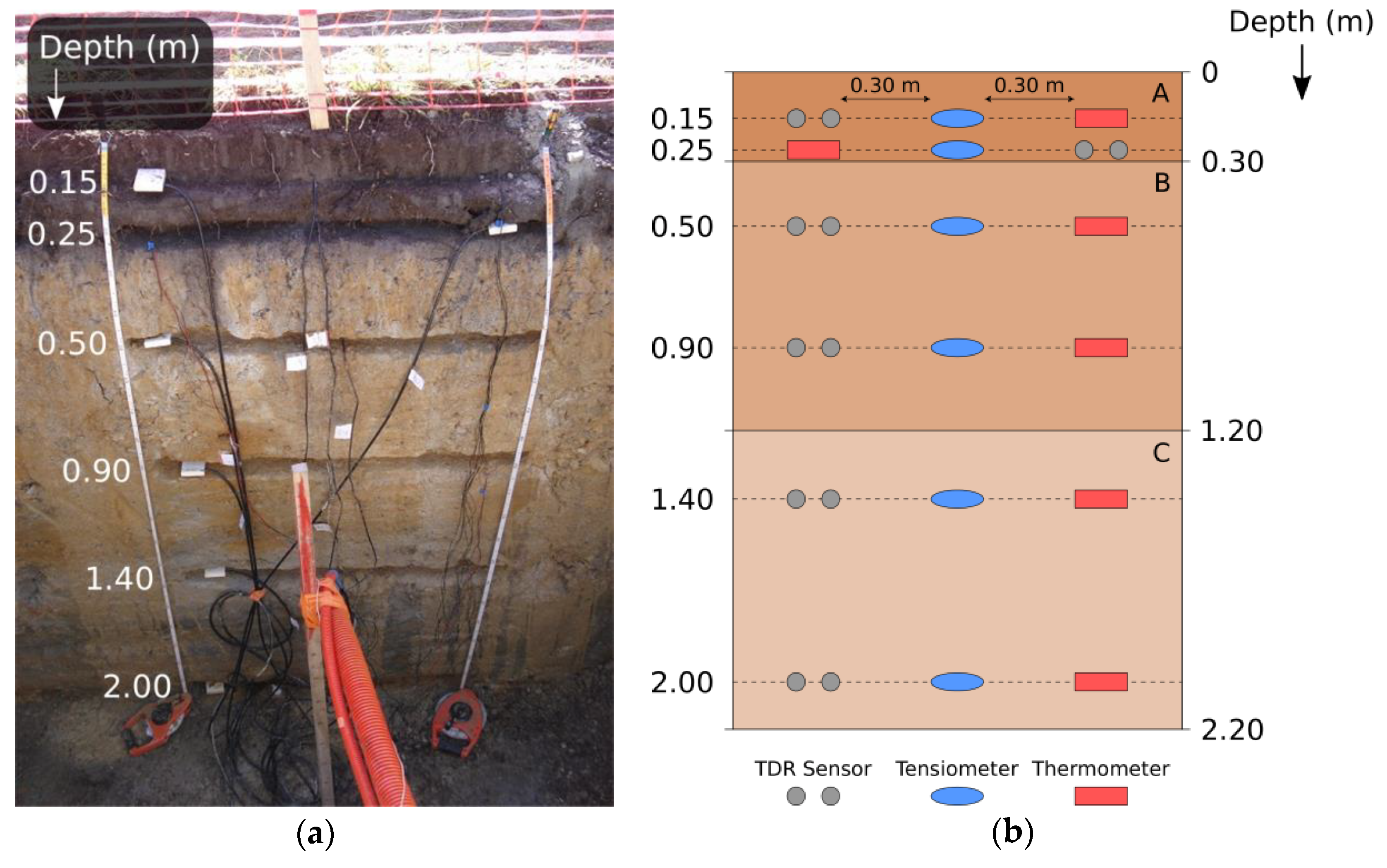
Figure 1. Geographical and geological situation of the Ploemeur Hydrological Observatory (modified from [23]).
Water 12 01230 g001
Figure 2. (a) Picture of the pit dug in 2012 with sensors installed [51]; (b) cross-section schematic showing sensor positions and horizons (A, B, C) described in Table 1.
Water 12 01230 g002
Figure 3. Schematic of acquisition setup and picture during an infiltration event. The solid pink line along the pit area corresponds to the plane including the buried sensors.
Water 12 01230 g003
Figure 4. Volumetric water content (θ), matric water potential (Ψm), and temperature (T) throughout the experiment as recorded from the sensors at different depths. Markers indicating starting times of electrical resistivity tomography (ERT) and seismic acquisitions are shown on each curve. Gray shadings correspond to the periods of water infiltration.
Water 12 01230 g004
Figure 5. Pseudo-sections of apparent resistivity for (a) NS and (b) WE lines showing the background, 2nd, 5th, and 11th acquisitions.
Water 12 01230 g005
Figure 6. Background ERT inversions for (a) NS and (b) WE lines. Black points at the surface indicate electrode positions.
Water 12 01230 g006
Figure 7. ERT time-lapse inversions for (a) NS and (b) WE lines showing the relative change in ρ. Black points at the surface indicate electrode positions, and the dashed black lines delimit the infiltration area.
Water 12 01230 g007
Figure 8. Seismic traces inside the infiltration area from shot No. 3 (x = 1.9 m) along the NS line. We show the traces from the background, 5th, and 11th acquisitions and observe a clear positive shift in P-wave first arrival times.
Water 12 01230 g008
Figure 9. Picked traveltime differences between the nth acquisition (tn, for n = 2, 5, 8, 11) and background acquisition (t1) for (a) NS and (b) WE lines for every shot-geophone pair. The black dashed lines delimit the geophone positions inside the infiltration area.
Water 12 01230 g009
Figure 10. Background P-wave seismic refraction tomography model for (a) NS and (b) WE lines. Black points at the surface indicate geophone and shot positions.
Water 12 01230 g010
Figure 11. Seismic time-lapse inversions for (a) NS and (b) WE lines showing the relative change in VP. Black points at the surface indicate geophone and shot positions, and the dashed black lines delimit the infiltration area.
Water 12 01230 g011
Figure 12. Electrical resistivity (ρ) versus water saturation (Sw) inside the infiltration area at the depths of the TDR sensors. The data points come from both NS and WE lines. The black solid lines correspond to resistivity models described in the text.
Water 12 01230 g012
Figure 13. P-wave velocity (VP) versus water saturation (Sw) inside the infiltration area at the depths of the TDR sensors. The data points come from both NS and WE lines. The solid lines correspond to velocity models described in the text for 100% quartz (black) and 100% clay (gray).
Water 12 01230 g013
Figure 14. Isochrones showing a given percentage of relative change in electrical resistivity (ρ) and P-wave velocity (VP) and their evolution with acquisition for (a) NS and (b) WE lines. The dashed black lines delimit the infiltration area and the gray arrows indicate line crossings.
Water 12 01230 g014
Figure 15. P-wave velocity (VP) versus resistivity (ρ) inside the infiltration area at the depths of the TDR sensors. The data points come from both NS and WE lines at the background and last (11th) acquisitions.
Water 12 01230 g015
Table 1. Soil characterization from pit samples after [51].
HorizonHorizon Limits (m)Clay (%)Silt (%)Sand (%)Soil TypeSampling Depth (m)ρb (g/cm3)ϕ (%)
A0–0.37.5085.147.36Silt0.15
0.25
1.04 ± 0.02
1.31 ± 0.05
50
50
B0.3–1.22.7668.3928.85Silty loam0.50
0.90
1.79 ± 0.01
1.71 ± 0.02
30
30
C1.2–22.3862.4332.81Silty loam1.40
2.00
1.86 ± 0.02
1.65 ± 0.05
30
30

