Article

Spatial and Temporal Characterization of Escherichia coli, Suspended Particulate Matter and Land Use Practice Relationships in a Mixed-Land Use Contemporary Watershed

by
Fritz Petersen
1,* and
Jason A. Hubbart
1,2
1
Division of Plant and Soil Sciences, Davis College of Agriculture, Natural Resources and Design, West Virginia University, Agricultural Sciences Building, Morgantown, WV 26506, USA
2
Institute of Water Security and Science, Schools of Agriculture and Food, and Natural Resources, Davis College of Agriculture, Natural Resources and Design, West Virginia University, 3109 Agricultural Sciences Building, Morgantown, WV 26506, USA
*
Author to whom correspondence should be addressed.
Water 2020, 12(5), 1228; https://doi.org/10.3390/w12051228
Submission received: 12 March 2020 / Revised: 18 April 2020 / Accepted: 23 April 2020 / Published: 25 April 2020

Abstract

:
Understanding land use practice induced increases in Escherichia (E.) coli and suspended particulate matter (SPM) concentrations is necessary to improve water quality. Weekly stream water samples were collected from 22 stream gauging sites with varying land use practices in a representative contemporary mixed-land use watershed of the eastern USA. Over the period of one annual year, Escherichia (E.) coli colony forming units (CFU per 100 mL) were compared to suspended particulate matter (SPM) concentrations (mg/L) and land use practices. Agricultural land use sub-catchments comprised elevated E. coli concentrations (avg. 560 CFU per 100 mL) compared to proximate mixed development (avg. 330 CFU per 100 mL) and forested (avg. 206 CFU per 100 mL) sub-catchments. Additionally, agricultural land use showed statistically significant relationships (p < 0.01) between annual E. coli and SPM concentration data. Quarterly PCA biplots displayed temporal variability in land use impacts on E. coli and SPM concentrations, with agricultural land use being closely correlated with both pollutants during Quarters 2 and 3 but not Quarters 1 and 4. The data collected during this investigation advance the understanding of land use impacts on fecal contamination in receiving waters, thereby informing land use managers on the best management practices to reduce exposure risks.

1. Introduction

Fecal pollution is the greatest contributor to water borne disease human morbidity and mortality rates globally [1]. Freshwater fecal pollution and subsequent increases in pathogenic bacteria (e.g., Escherichia (E) coli), cause disease outbreaks, including diarrhea, urinary tract infections, respiratory illness and pneumonia [2,3]. The World Health Organization reported that 2.2 million deaths are caused by diarrhea annually, due to the consumption of fecal contaminated water [1]. An improved understanding of factors leading to increased fecal contamination in receiving waters will be useful in reducing outbreaks of waterborne disease and improving water quality. Furthermore, understanding the factors impacting the health and exposure risks of fecal pollution can be used to decrease the threat posed by fecal organisms. For example, the environmental persistence of fecal microbes can be extended when occurring with suspended particulate matter (SPM) [4,5]. Therefore, monitoring SPM in conjunction with fecal pollution can provide greater insight into water quality, through more accurate assessments of the persistence of fecal microbes.
Suspended particulate matter (SPM), defined as heterogeneous aggregates of mineral fragments, organic matter and microbial fractions, comprises the greatest water pollutant by volume globally [6]. Excess SPM in freshwater can impact water quality by decreasing the amount of transmitted light, thereby restricting or eliminating the photosynthesis of aquatic plants and dramatically influencing the aquatic food chain [7,8]. Therefore, understanding the factors influencing fluxes in SPM (e.g., land use practices) is important from an ecosystem management perspective. Additionally, increases in SPM can clog the gills of fish, thus lowering resistance to disease and decreasing developmental growth rates [7] while also elevating water temperatures, thereby disrupting the metabolic processes of various aquatic biota [8]. Thus, changes in SPM concentrations in receiving waters can entail serious consequences for various aquatic organisms. SPM can also act as a conveyance system for other pollutants including heavy metals, chemicals and pathogens, including fecal microbes (as discussed above) [8,9,10,11,12]. Insofar as excess sediment can be harmful to aquatic ecosystems, too little sediment can also be harmful, leading to the scouring of river channels, erosion and reduced nutrient inputs [8,13]. Consequently, understanding the factors leading to increases or decreases of SPM in receiving waters is important from a water quality perspective [14].
Previous work investigating fecal contamination and SPM reported statically significant, Pearson’s product moment, correlations (r > 0.9) between the two pollutants [15]. Moreover, the strength of the relationships between fecal pollution and SPM reported in previous work [15,16] has led to speculation that SPM concentrations (and the turbidity caused by SPM) can potentially serve as a proxy for fecal contamination [16]; however, this is yet to be verified. The relationship between fecal contamination and SPM has been attributed to similar transport processes influencing both pollutants during run-off events [17], including similar in-stream transport physics [18], and the sorption of fecal microbes to SPM [4,5]. Additionally, certain land use practices can simultaneously elevate both SPM and fecal microbe concentrations in receiving waters [19,20]. For example, agricultural land use practices are commonly associated with increased fecal (e.g., E. coli) and SPM concentrations relative to other land use types [19,20,21,22]. This is often related to the presence of livestock [23], with livestock population density being correlated to fecal indicator organism concentration [24]. Manure application in agricultural areas has also been linked to increased concentrations of fecal microbes in receiving waters [4]. Conversely, agricultural practices such as soil tillage and soil exposure yield increased SPM concentrations in the receiving waters of agricultural areas [19,21]. Differing land use practices in a given area (watershed) can therefore account for differing E. coli and SPM concentrations in receiving waters and should thus be accounted for when monitoring these pollutants.
Despite the progress of previous research, knowledge gaps regarding the relationship between fecal contamination and SPM remain. For example, few studies investigated the relationships between SPM and fecal contamination in mixed land use settings. Furthermore, the majority of studies included limited sampling locations [20,25] and tended to occur in areas of similar land use types [16,26], or were controlled laboratory simulations [27]. Additionally, previous work on fecal contamination typically focused on storm events and therefore report disproportionately elevated fecal concentrations in receiving waters [28]. Clearly, knowledge regarding fecal concentrations outside of storm events is lacking, creating challenges for proper management practices. Similarly, previous work investigating fecal concentrations in receiving waters typically utilized shorter (weeks or months) sampling periods [20], which fail to account for the seasonal variability in land use practices. For example, seasonal variability in agricultural land use practices can lead to changes in fecal microbe concentrations in receiving water, particularly in areas where manure is applied [29]. Manure is typically only applied in specific seasons, thereby leading to corresponding increases in the fecal contamination of associated receiving waters during these seasons [29]. Therefore, a study design capable of distinguishing the effects of different land uses and seasonality would be useful for investigating fecal contamination and SPM in receiving waters and for better informing water resource managers.
Previous studies have used many different study design methods, including different sampling regimes, to advance the understanding of E. coli regimes. Study designs have included laboratory based designs comprising simulations [30] and field based designs comprising event based sampling [31], periodic sampling [32], stochastic sampling [33] and nested-scale experimental watersheds [20]. The nested-scale and paired experimental watershed study design is a method that has been successfully used to quantify the effects of land use practices on receiving waters in mixed land use settings [34,35,36,37,38,39,40]. Nested watershed study designs divide a larger watershed into a series of sub-catchments to investigate the influence of land use practices on the environmental variables of interest [35,37,41,42,43]. Sub-catchment delineation isolates different land use practices and hydrologic characteristics [41]. Paired watersheds comprise at least two physiographically similar watersheds (control and treatment) from which data are collected [41]. The study design enables the identification of the influence and cumulative effect of various land use practices on the response variable of interest through the quantification of the influencing processes observed at the sub-catchment scale [44]. Therefore, the approach allows for the effective disentanglement of factors (e.g., land use practices and SPM) that influence a given response variable of interest (e.g., fecal microbe concentration), thus providing quantitative information regarding hydrologic and water quality regimes related to specific land-uses [41]. Given its proven application in over a century of studies, the nested-scale and paired experimental watershed study design is an accepted optimal study design for investigating current knowledge gaps regarding fecal contamination, SPM and land use practices.
The Appalachian region of the USA is well-suited for researching knowledge gaps concerning fecal contamination, SPM and land use practices. The region is representative of many locations globally given that it suffers from widespread, frequent, and problematic fecal pollution [45]. Additionally, Appalachia is physiographically diverse, encompassing distinct Northern, Central and Southern regions, consisting of dissimilar geographic, climatological, and ecological characteristics [46]. For example, the temperate climate and well-distributed year-round rainfall characteristics of Central Appalachia [47] are similar to those of areas such as Uruguay or Southern Brazil [48], and many other locations. Conceivably, other temperate areas comprising year-round precipitation (e.g., Uruguay) will benefit from research conducted in the Central Appalachian region as the results will be comparable and transferable. Furthermore, water quality is a primary concern in rural Appalachia as thousands of residents are exposed to water quality problems, specifically regarding microbial contamination [49]. Water quality problems in rural areas are exacerbated by inadequate wastewater treatment infrastructure, isolation due to geographically inaccessible terrain, and poverty [49]. Consequently, water quality is a primary concern, and insight into both SPM and fecal pollution (e.g., E. coli concentrations) is necessary to effectively inform policy makers and water resource managers regarding water quality to make the best management practice decisions in Appalachia and physiographically similar locations globally.
The overarching objective of the current investigation was to quantify fecal contamination (E. coli concentration) and SPM concentrations in receiving waters relative to differing land use practices from numerous sites in a mixed-land use contemporary watershed of Appalachia. Sub-objectives included (1) investigating the relationship between fecal microbe concentration (E. coli colony forming units) and SPM concentrations in receiving waters, and (2) determining the influence of quarterly (seasonal) changes on the relationship between E. coli and SPM. The study outcomes were to improve the understanding of the influence of land use practices on both fecal contamination and SPM pollution, providing land use managers with insight into factors influencing water quality in receiving waters.

2. Methods

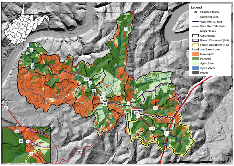
2.1. Study Site Description

This research took place in West Run Watershed (WRW) a 23 km2 mixed-land use urbanizing watershed located in Morgantown, West Virginia, USA. West Virginia’s climate varies between cold and humid with warm summers, to temperate and humid with hot summers [50]. In Morgantown, WV, located in Monongalia County (and including the WRW), the climate is characterized by the lack of a dry season, cold winters (mean monthly temperature < 0 °C) and warm-to-hot summers (mean monthly temperature > 22 °C) [50]. Historically (1981–2010), Morgantown received approximately 1060 mm of average annual precipitation, with the coldest (January) and driest (February) months having an average daily temperature of −0.4 °C and an average monthly precipitation of 66 mm, respectively [51]. Conversely, the warmest and wettest month (July) comprised an average daily temperature of approximately 23 °C and an average monthly precipitation of 117 mm [51].
West Run Creek, the primary drainage of WRW, is a third order tributary of the Monongahela River, and includes many land use practices including agriculture, urban and forested areas [22]. Based on the 2016 National Agriculture Imagery Program (NAIP) land use and land cover data, WRW includes 42.7% forested land use, 37.7% mixed development (urban and commercial areas) land use and 19.4% agricultural land use practices. West Run Creek is a narrow, moderately entrenched stream with multiple small floodplains [20,52]. The elevation of the headwaters of WRW is 420 m above mean sea level [22]. Conversely, the elevation of the confluence of WRW with the Monongahela River is 240 m above mean sea level [20]. The watershed includes relatively rugged terrain, featuring numerous Paleozoic era rock outcroppings [20]. The headwaters of WRW contain the most recent geological formation (Monongahela series) [20]. Two coal formations are also present in the watershed, namely the Upper Kittanning coal and the Pittsburg coal seam [20]. Historic mining of the Pittsburg coal seam negatively impacted water quality in WRW, particularly in the headwaters [53].
A nested-scale and paired experimental watershed study design [35,44,54,55,56] comprising twenty-two study sites (i.e., gauge sites) was implemented in 2017. Sampling sites (numbered in downstream order) were located in West Run Creek (#3, #4, #6, #10, #13, #18, #19, #21 and #22) and its first and second order confluence tributaries (#1, #2, #5, #7, #8, #9, # 11, #12, #14, #15, #16, #17 and #20) and included varying land use practices (Table 1; Figure 1). Both field surveys and GIS were used to identify the study sites and related sub-catchments. At the time of this investigation, forested land use was the predominant land use in WRW, accounting for 42.7% of the total land use practices in the watershed. Additionally, forested land use was the predominant land use type in all sub-catchments except #1, #11, #15, #16 and #20. Sub-catchments #1, #15 and #20 were primarily mixed development, whereas sub-catchments #11 and #16 where primarily agricultural (Table 1). Conversely, 85.84% of sub-catchment #17 was forested land use, the highest among the sub-catchments. This sub-catchment, which served as a reference sub-catchment (control) for the current work, also comprised 9.4% agricultural and 4.8% mixed development land use practices. Sub-catchment #17 is, therefore, considerably different to sub-catchment #12 (34.5% forested, 33.7% agriculture and 31.7% agriculture) despite both comprising predominantly forested land use practices. In general, at the time of the investigation, mixed development comprised the second largest percentage of land use practices (37.7%) and agricultural land use practices accounted for the lowest percentage of land use practices (19.4%) in WRW.

2.2. Data Collection

Climate data collected for the current work included precipitation (Campbell Scientific TE525 Tipping Bucket Rain Gage), average air temperature, relative humidity (Campbell Scientific HC2S3 Temperature and Relative Humidity Probe), and average wind speed (Campbell Scientific Met One 034B Wind Set instrument). Data were recorded at a 3 m height during the study period (2 January 2018–1 January 2019) by a climate station located within approximately 30 m of Site #13 (Figure 1).
For the current work, weekly water grab-samples were collected as per Petersen et al. [20], Hubbart et al. [57], Kellner and Hubbart [43], and Zeiger and Hubbart [42,58] from each monitoring site (stream order ≤ 3). Water sample collection was initiated at 09:00 at Site #1 and continued in numerical order of sites. Sites #9 and #10 were exceptions, as they were sampled before Sites #7 and #8, due to their location relative to other sites (Figure 1). The proximity of Sites #9 and #10 to Site #6 meant that overall sampling time was reduced by sampling them after Site #6, increasing the comparability of the samples during sample processing. The sampling period for the study (2 January 2018–1 January 2019, thus 53 weeks) was one calendar year to account for seasonal variability in the E. coli concentration and SPM data. Notably, the sampling period was longer than in typical studies on fecal contamination [59,60], allowing for a comprehensive quantification of fecal contamination (E. coli) regimes at sub-catchment mixed-land-use scales. The high-resolution study design resulted in a total of 1166 spatio-temporally delineated fecal contamination (E. coli) concentration and SPM concentration values.
Following collection, the samples were transported to the Interdisciplinary Hydrology Laboratory, located in the Davis College of Agriculture, Natural Resources and Design at West Virginia University, for analyses. In the laboratory, water samples were refrigerated (at 3.3 °C), and gravimetric analyses (vacuum filtration) were conducted as per the American Society for Testing and Materials, test number D 3977-97, [61] within a few days of collection to determine the mass of suspended particulate matter (SPM). Additionally, fecal contamination was quantified immediately upon arrival at the laboratory using Escherichia (E) coli as an indicator organism, as per previous work [20,62]. E. coli coliform forming units (CFU) were enumerated using the U.S. Environmental Protection Agency (EPA) approved Colilert test [63], developed by IDEXX Laboratories Inc. The applied method used an MPN approach to estimate the E. coli CFU concentration; therefore, E. coli concentration data were referred to as CFU, not MPN, during the investigation. The test, included in Standard Methods for Examination of Water and Wastewater was developed to estimate fecal concentrations in water samples without requiring sample dilution [63,64]. A combination of Colilert’s Defined Substrate Technology nutrient-indicator (ONPG), and a selectively suppressing formulated matrix created low chances of recording inaccurate results (chance of reporting false positives ±10%). With this test, most non-target organisms are unable to grow given that they lack the enzyme to metabolize the provided carbon source (ONPG) [63]. The formulated matrix selectively suppresses the few non-target organisms that can metabolize ONPG [63]. The number of E. coli colony-forming units (CFU) per 100 mL of sampled water was estimated using the Quanti-Tray system, comprising 96 total wells: 48 large wells (49, including the overflow well) and 48 small wells [63]. The Colilert (ONPG) substrate was added to 100 mL of sampled water, sealed in the Quanti-Tray, and incubated at 35 °C for 24 hours, as per Colilert’s instructions [29]. Following incubation, fluorescing (positive for E. coli) wells were quantified using a UV light and converted, with a 95% confidence interval, into a concentration of E. coli (CFU per 100 mL) using the Quanti-Tray Most Probable Number (MPN) table. The E. coli concentration range resultant from the Quanti-Tray/MPN table method was <1 to 1011.2 CFU. Therefore, E. coli concentrations in excess of 1011 CFU per 100 mL could not be accurately estimated. This limitation was an allowable shortcoming of the current work given the focus on the weekly detection of small E. coli concentrations occurring between storm events.

2.3. Data Analysis

Descriptive statistics were generated for E. coli and SPM concentrations and aggregated for the study period. Average percentage differences between sites were determined by comparing the average SPMs and average E. coli concentrations between sites. Statistical analyses were conducted using Origin Academic 2018 (OriginLab Corporation). Normality testing was completed using the Anderson Darling Test [65]. Land use practices were reclassified (lumped) into three major categories prior to analysis, namely mixed development, agriculture, and forested [20]. Mixed development constituted roads, impervious surfaces, mixed developments and barren areas. Agriculture included low vegetation, hay pasture and cultivated crops. Forested land use included mine grass, forest, mixed mesophytic forest, dry mesic oak forest, dry oak (pine) forest and small stream riparian habitats. Annual data were also analyzed in four quarter data subsets, comprising all weekly samples collected in three month blocks starting on January 1st, 2018, to analyze seasonal variation. Thus, Quarter 1 included 2 January 2018–27 March 2018 (winter), Quarter 2 included 3 April 2018–26 June 2018 (Spring), Quarter 3 included 3 July 2018–25 September 2018 (summer), and Quarter 4 included 2 October 2018–1 January 2019 (fall). Spearman correlation tests, with a significance threshold of α = 0.05 [66], were used to analyze the relationship between E. coli concentration, suspended sediment, and land use practices at all twenty-two sites, as per Petersen et al. [20] for the complete annual data set and the four quarterly data subsets. Finally, principal component analysis (PCA) was used to investigate the relationships between E. coli concentrations, SPM and land use practices (presented in biplots) across all 22 sampling locations for the annual data set and the four quarterly data subsets.

3. Results and Discussion

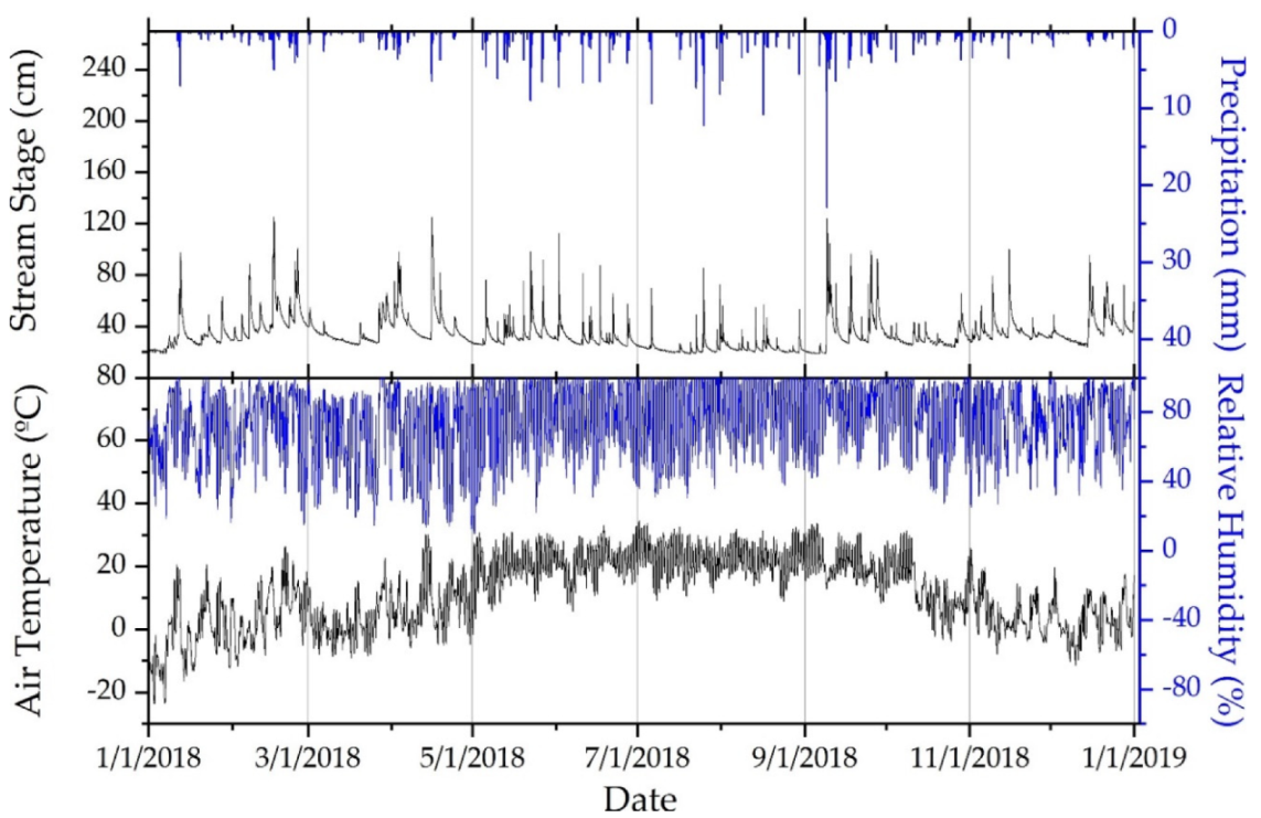
3.1. Climate during Study

Total precipitation was 1378 mm in 2018 in WRW. This was approximately 20% more precipitation than the historic annual average (1096 mm) dating back to 2007 [67]. September (186 mm) and October (47 mm) were the wettest and driest months, respectively, during 2018 (Figure 2). Approximately 14% of the annual precipitation was received in September. This was more than double the historic average precipitation (80 mm) for that month [67]. The average air temperature, during the study period was approximately 12 °C, which is close to the historic average of 11 °C [67]. July (22 °C) and January (−4 °C) comprised the warmest and coldest average monthly temperatures, respectively, in WRW during 2018. Relative humidity was characteristically high during 2018 (Figure 2), comprising a yearly average of 76%. Generally, climate during the period of study (2 January 2018–1 January 2019) was predictably variable and consistent with historic trends (Figure 3), including humid and warm weather during the summer months, with temperatures decreasing over the transition to winter (Figure 3). As is typical of the region, there was no dry season; however, large precipitation events during Quarters 2 (spring; e.g., May 6th: 24 mm) and 3 (summer; e.g., September 9th; 60 mm) resulted in greater quarterly (seasonal) variation in precipitation (Figure 2) [67]. Quarters 2 and 3 (spring and summer; 850 mm) therefore received 67% more precipitation than Quarters 1 and 4 (winter and fall; 510 mm).

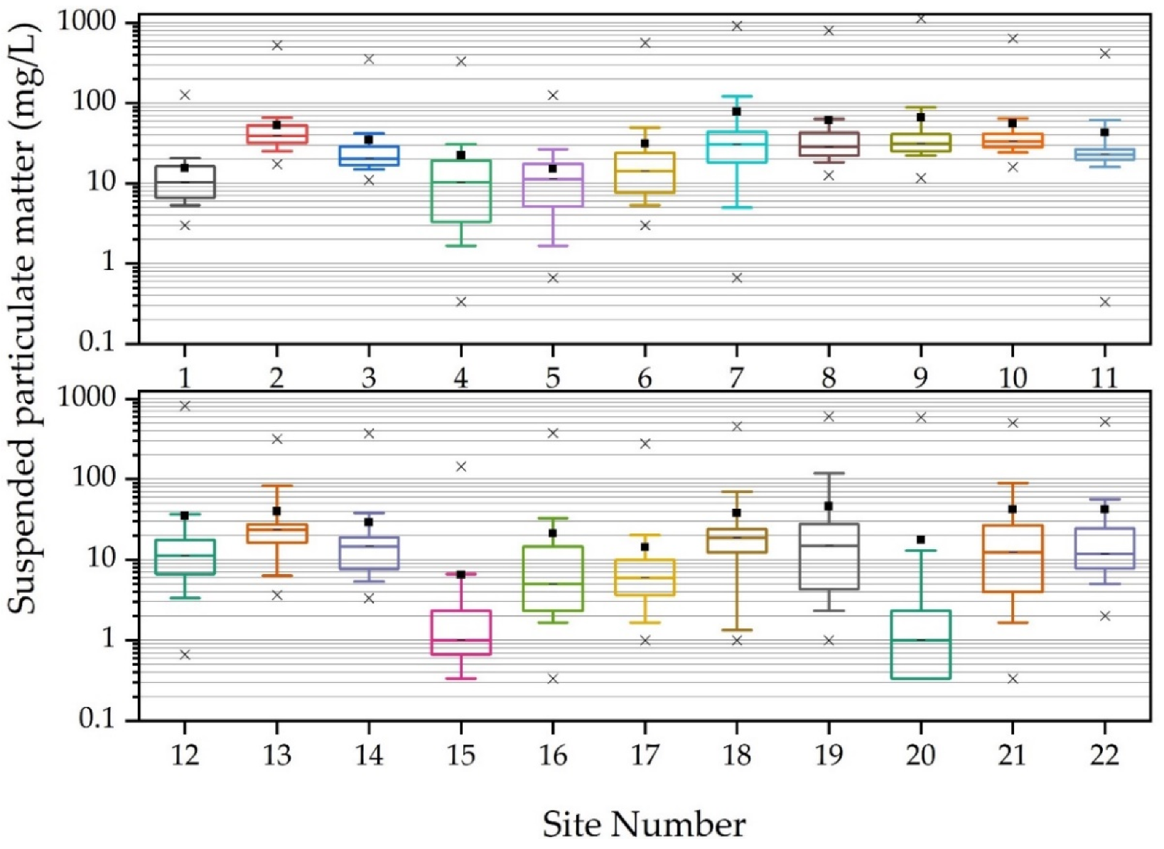
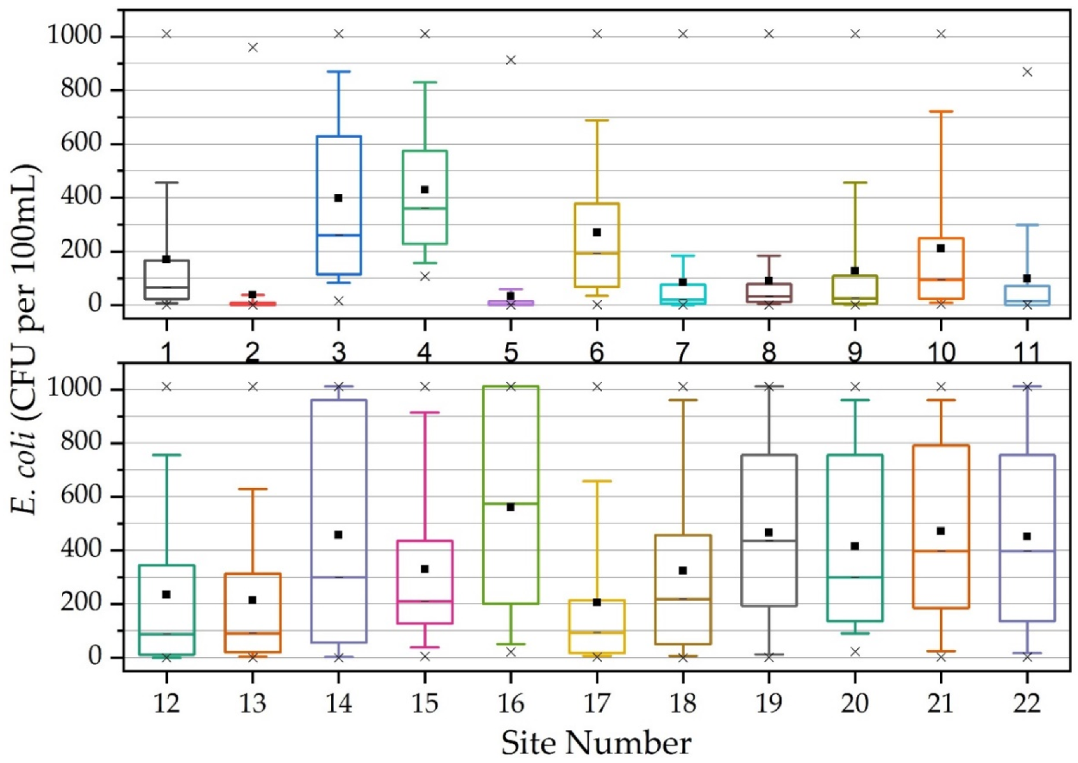
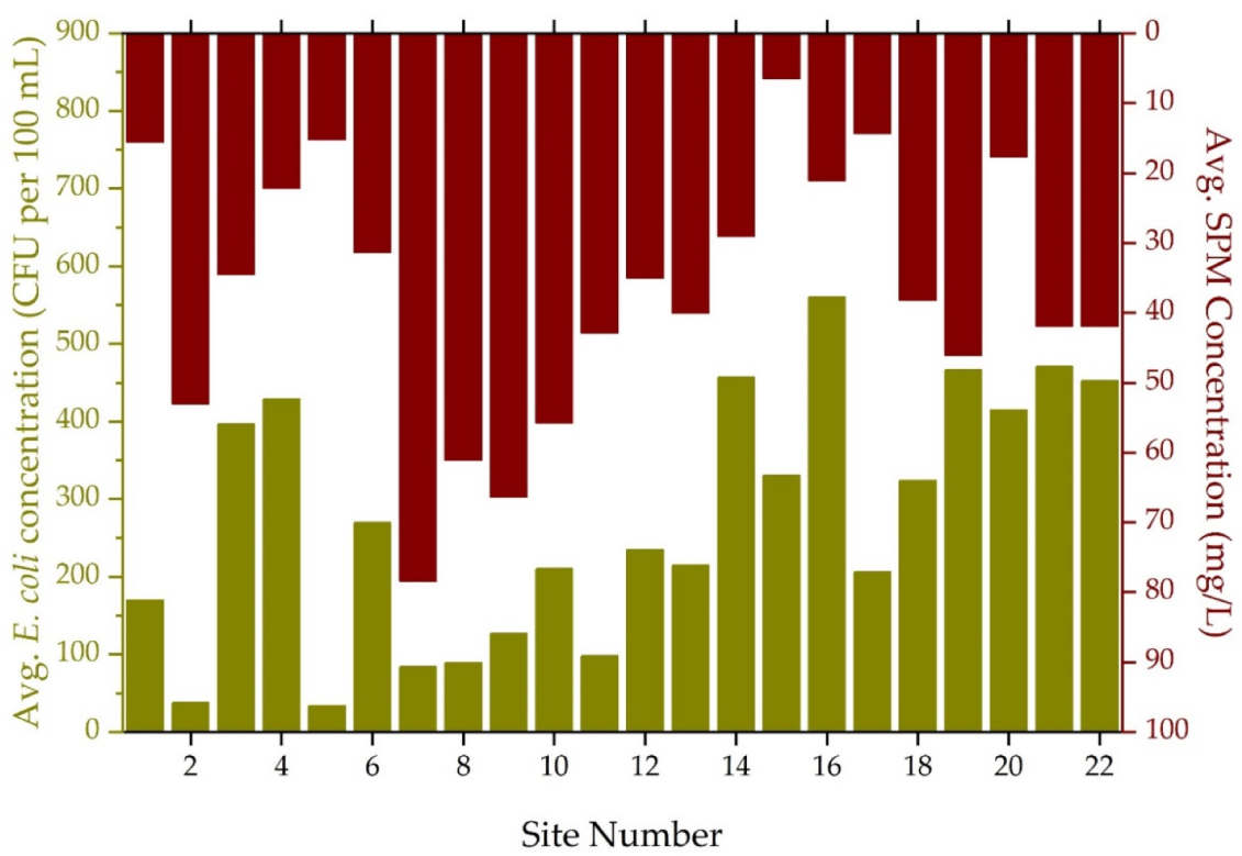
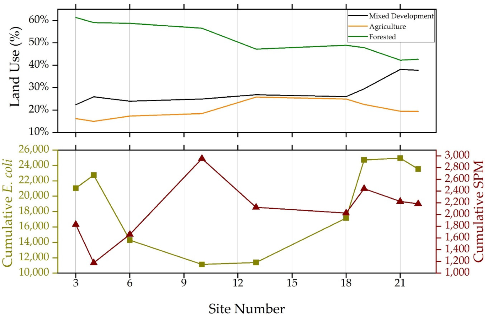
3.2. Annual Suspended Particulate Matter, E. coli Concentrations and Land Use Practices

The results showed that forested sub-catchments had the highest average (Site #7; 55% forested; 78.4 mg/L), maximum (Site #9; 53% forested; 1140 mg/L) and minimum (Site #8; 52% forested; 12.7 mg/L) SPM concentrations (Table 2; Figure 3). Notably, these sub-catchments constituted one of the paired watersheds of the paired study design and were in close proximity to each other (Figure 1). Consequently, these sub-catchments were subject to similar land use activities and processes leading to elevated SPM in this region of the watershed. For example, the agricultural land use practices in the headwaters of sub-catchments #7 and #8 (Figure 1) could have elevated the SPM in the entire paired catchment (Sites #7, #8 and #9) as previous work has reported increased SPM in agricultural areas [19,20,21,22]. SPM concentrations were also elevated in West Run Creek (combined average of sites in West Run Creek, 39 mg/L) relative to sites located in the first and second order confluence tributaries (combined average, 35 mg/L) (Table 2; Figure 3). The increased SPM in West Run Creek was attributable to (1) the greater volumetric streamflow in West Run Creek relative to in its tributaries, as increased streamflow can increase the SPM concentration [68]; and (2) increased SPM sources due to an increased drainage area relative to its tributaries (23 km2 and 15 km2 respectively) (Table 1; Figure 1). Conversely, SPM concentrations were decreased in mixed development sub-catchments (Sites #15: 70% mixed development and #20: 89% mixed development) comprising the lowest average (6.5 mg/L), lowest median (1 mg/L), and lowest minimum (0 mg/L) (Table 2; Figure 3). Site #15 also had low SPM concentrations during previous work conducted in the WRW, thereby supporting the results from the current investigation [20]. Mixed development areas can comprise decreased exposed soil surfaces and subsequent reductions in the SPM sources relative to other land use types, which can account for the decreased SPM concentrations [69].
The study results showed that E. coli concentrations were the highest at sub-catchments comprising the greatest percentage agricultural land use area (Site #16: 59% agricultural). These results are similar to those of previous investigations in WRW reporting increased E. coli concentrations in agricultural land use sub-catchments [20]. This predominantly agricultural sub-catchment comprised the highest average (560 CFU per 100 mL) and median (575 CFU per 100 mL) (Table 3; Figure 4) E. coli concentrations over the period of investigation. Previous investigations in the USA (California and Ohio) reported increased fecal contamination with agricultural land use practices [31,70], and a significant correlation (p < 0.04) between agricultural land use and E. coli concentrations [20], thereby supporting the results recorded during the current work. The lowest E. coli concentrations were recorded at two forested sites (Site #2: 74% forested and Site #5: 51% forested) comprising the lowest median (3 CFU per 100 mL) and average (34 CFU per 100 mL) amongst the sites respectively (Table 3; Figure 5). These two sites, and the forested sub-catchments comprising one of the paired watersheds (Sites #7, #8 and #9) located in the headwaters of WRW (Figure 1), were heavily impacted by acid mine drainage (AMD) from historic mining activities [20,22,53], which likely, at least in part, explains the low E. coli concentrations observed at these sites. This is an important finding given that previous studies showed that AMD lowers the pH of receiving waters [71] and that the current results indicate that AMD may also lower E. coli concentrations. Forested sites generally had lower E. coli concentrations (e.g., Site #17: 86% forested; average E. coli concentration: 206 CFU per 100 mL) during the study period than sites comprising other land use practices (e.g., Site # 20: 89% mixed development; average E. coli concentration: 415 CFU per 100 mL) (Figure 4). These results align well with previous studies reporting decreased fecal contamination in forested areas [70] and are attributable to the increased quality of receiving waters in forested areas [72]. Consequently, both forested land use practices and AMD lowered E. coli concentrations in WRW during the investigation. Notably, the low average E. coli concentrations recorded during the study period (2 January 2018–1 January 2019), specifically in the headwaters, affirms the study objective of analyzing samples collected between storm events that comprise lower E. coli concentrations. Additionally, in no other study has there been such high spatial and temporal resolution sampling over a full annual year. This allowed for a more comprehensive analysis of E. coli concentration regimes and relationships with SPM and land use, including accounting for seasonality, than is available in the literature surrounding contemporary mixed land use watersheds. The current study therefore lends greatly needed confirmation through high spatial and temporal resolution of previous studies.
E. coli concentrations showed a general increase from the headwaters of WRW to the confluence of the Monongahela River, with larger average concentrations typically being observed in the lower portions of the watershed (Figure 5). In the current work, AMD may account for the lower E. coli concentrations in the upper watershed (as discussed above). However, in the lower elevations of WRW, land use practices may be the predominant factor influencing E. coli concentrations. For example, in West Run Creek (Sites #13–#21), there was a notable increase in cumulative E. coli concentrations and a simultaneous increase in agricultural and mixed development land use practices (Figure 6). Previous work reported on the increased fecal contamination associated with increased agricultural and urban areas [31,70,73,74], commonly attributed to increased sources (livestock and manure) [23] and increased (concentrated flow) run-off during precipitation events, respectively [73], and urban stream syndrome [75], thereby supporting the results from the current investigation. The inter-site relationship between E. coli concentrations and SPM was not clearly discernable based on average values (Figure 5) or cumulative values in West Run Creek (Figure 6), as increases in SPM were not always accompanied by similar increases or decreases in E. coli between the different sampling locations. A potential explanation for these results may be that SPM and E. coli concentrations are affected by different factors at different sites (e.g., geochemistry, land use and antecedent soil water conditions). Thus, in WRW, there may exist a spatial disconnect regarding the factors influencing E. coli concentrations and subsequently impacting the relationship between E. coli and SPM in the watershed. To account for the spatial disconnect, site specific analysis of E. coli and SPM correlations, including separate analysis for different time periods in the year (quarters), was required to improve the current understanding regarding this relationship and to assess the use of SPM as a proxy for fecal contamination.

3.3. Quarterly Suspended Particulate Matter, E. coli Concentrations and Land Use Practices

Average E. coli and SPM concentration data showed notable temporal variation during 2018, based on quarterly analysis (Figure 7). E. coli concentrations were elevated during Quarter 2 (spring; 3 April 2018–26 June 2018) and Quarter 3 (summer; 3 July 2018–25 September 2018) of 2018, coinciding with the warmer spring and summer months (average maximum daily temperatures: Quarters 2 and 3 = 26 °C; Quarters 1 and 4 = 9 °C) of the year and higher stream flows induced by larger and more frequent precipitation events (Figure 3). Previous work noted correlations between elevated air temperatures and E. coli concentrations in freshwater [74], thereby supporting the results from the current work reporting greater E. coli concentrations during warmer months. Furthermore, the second and third quarters included some of the largest precipitation events of 2018 (Figure 3). These precipitation events could, at least in part, account for the elevated E. coli concentrations recorded during this time period, as previous work linked precipitation events to elevated E. coli concentrations in receiving waters [32,74]. Conversely, the highest average SPM concentrations were recorded during Quarters 1 (winter) and 2 (spring), with average concentrations decreasing during the second half of the year (Figure 7). The high SPM recorded during this time period may be attributable to decreased vegetation cover throughout WRW, leading to increased exposed soil surfaces, owing to the seasonal changes in vegetation (i.e., many plant species senesce during the cold winter months) [76,77]. Once vegetation throughout WRW increases during Quarter 3 (summer), exposed soil surfaces and sources of SPM become more limited. Quarter 4 (fall) comprised low E. coli and SPM concentrations. During this time period, WRW received less precipitation than in the preceding quarters (Figure 2), which could have limited the transport of pollutants (i.e., E. coli and SPM) to receiving waters [78]. Additionally, E. coli concentrations in the receiving water could have been suppressed by the colder temperatures [79] and decreased nutrient availability owing to the drier antecedent conditions and greater infiltration [77,80].

3.4. Non-Parametric Statistical Results

Normality test results indicated that the E. coli concentration data were non-normally distributed, thus Spearman correlation coefficients (nonparametric version of the Pearson product moment correlation) were used to quantify the relationships between E. coli concentration, SPM concentration, and land use at each site. E. coli concentrations and SPM concentrations were not significantly correlated at all sites; however, nine of the 22 sites (Sites #4, #7, #8, #9, #11, #15, #16, #17 and #20) did have significant correlations (Table 4). Notably, Sites #7, #8 and #9, which had the highest SPM during the investigation (Table 2; Figure 3), displayed statistically significant positive correlations (p < 0.01 for all three sites) between E. coli concentrations and SPM concentrations. Based on these relationships, SPM may serve as a relatively accurate proxy for E. coli concentrations in similarly physiographic catchments. Mixed development and forested sub-catchments did not display consistent significant correlations (p < 0.05) between E. coli and SPM concentrations. For example, Sites #15 (70.3% mixed development) and #17 (85.8% forested) both comprised statistically significant relationships between SPM and E. coli concentrations (p < 0.01and p < 0.05, respectively) despite comprising different predominant land use practices. However, Site #1 (53.2% mixed development) and Site #5 (51.1 % forested) displayed statistically insignificant correlations, despite including approximately similar dominant land use practices to Sites #15 and #17. As discussed in the preceding sections, AMD in the headwaters of WRW could be affecting E. coli concentrations, thereby creating inconsistency in the correlations between the E. coli and SPM concentrations. Therefore, the E. coli and SPM correlation results imply a spatial disconnect in terms of the influence of land use practices—in particular, mixed devolvement and forested areas—on the use of SPM as a proxy for fecal contamination. Notably, it seems likely, based on these results, that legacy effects (AMD) of historic land use practices (coal mining) may be impacting E. coli concentrations and affecting the observed relationships between E. coli and SPM concentrations. Conversely, both of the predominantly agricultural sites (Site #11 and #16) displayed significant correlations between SPM concentrations and E. coli concentrations, supporting previous work that reported elevated E. coli and SPM concentrations in the receiving waters of agricultural areas [19,20]. Therefore, in agricultural areas, SPM could be implemented as a proxy for E. coli with greater accuracy and less difficulty than in other land use areas.
Explanatory variables that account for the maximal variance in a data set can be identified via principle component analysis (PCA), through the computation of multiple principal components and their respective Eigenvalues [81]. Components comprising the highest Eigenvalues are assumed principal components, given that Eigenvalues represent the variance of the data in that direction [81]. A principle component is a linear function of the variables in an original data set that successively maximize variance and that are uncorrelated with each other [82]. Multiple principal components are typically calculated and ranked based on their Eigenvalues as most data cannot be well-described by a single principal component [81]. For the current work, the results showed three principal components with Eigenvalues exceeding 1 (an accepted threshold of importance [22,83]), including Principal Component 1 (Eigenvalue = 1.83), Principal Component 2 (Eigenvalue = 1.22) and Principal Component 3 (Eigenvalue = 1.17). These three principle components explained approximately 85% of the cumulative variance of the data set. Conversely, Principal Components 4 and 5 accounted for approximately 16% and 0% of the variance of the data set. For the current work, the principle component biplots showed distinct spatial distributions for study sites along Principal Components 1 and 2 (Figure 8). The idealized biplot vector space defined by Principal Components 1 and 2 is characterized by the grouping of the sites. Given these results, it can be concluded that land use practices are the primary factors influencing the grouping of the data in the biplot, given the similarity of the sites in terms of geology, topography and climate, and their close proximity to each other [52]. The strongest correlation illustrated by the biplot is between SPM concentration and agricultural land use practices (Figure 8). However, E. coli concentration is also closely related to both, attributable to agricultural land use practices (i.e., the rearing of livestock, manure application, soil tillage and increased exposed soil surfaces), as discussed in the preceding sections and reported by previous investigations [19,20,21,22,23]. Ultimately, the PCA results were analogous to the Spearman correlation coefficient results, indicating that SPM could potentially serve as proxy for E. coli in agricultural areas, especially during periods with lower levels of fecal contamination between storm events.
The Spearman correlation test results based on the quarterly analysis of data indicated predictable temporal variation in the correlation between E. coli and SPM concentrations, with only Site #9 showing significant correlations (p < 0.05) throughout all four quarters (p < 0.01 Quarters 1 to 3; p = 0.02 Quarter 4) (Table 5). Quarter 1 displayed the most significant correlations (10; Site #2, #7, #8, #9, #10, #11, #12, #13, #15, and #18), whereas Quarter 4 had the fewest significant correlations (two; Site #9 and #16) (Table 5). The temporal variation can be explained by the different impacts seasonal variation have on E. coli and SPM concentrations. For example, as discussed above, SPM concentrations will be influenced by changes in vegetation, with elevated concentrations typically occurring when vegetation cover decreases and decreasing as vegetation cover increases [76,77]. Therefore, elevated SPM concentrations can be expected during and immediately after the cold winter months, with decreased concentrations during the warmer summer months. Conversely, previous work linked elevated E. coli concentrations with warmer water (and air) temperatures [84,85,86]. Consequently E. coli concentrations can be expected to be elevated during the warmer summer months and decrease during the colder winter months. Ultimately, there is a temporal (seasonal) difference between periods of elevated SPM and E. coli concentrations. For example, Quarter 3 included the highest average (424 CFU per 100 mL) E. coli concentrations across all 22 sampling locations, while Quarter 1 comprised the lowest average (187 CFU per 100 mL) E. coli concentration. Thus, between Quarter 1 and 3 there was more than a 100% increase in average E. coli concentrations across the 22 sampling sites. Conversely, Quarter 1 had the highest average (55.7 mg/L) SPM across all 22 sampling locations, while Quarter 4 comprised the lowest average (18.2 mg/L) SPM. Consequently, there was more than a 65% decrease in average SPM, across the 22 sampling locations, between Quarter 1 and Quarter 4. These temporal differences, driven by changes in precipitation [78], antecedent conditions [87], seasonal land cover [76] or land use practices [29] may account for the variable E. coli and SPM concentrations correlations identified in Table 5.
The varying correlations displayed in Table 5 constitute important results regarding the use of SPM as a proxy for E. coli. Temporal changes in correlation significance indicate that SPM cannot be a consistently accurate proxy for fecal contamination throughout all the quarters (seasons) of a year. Even agricultural sub-catchments displayed insignificant correlations during certain quarters (Quarter 3 and 4 for Site #11 and Quarter 1 for Site #16), despite being significantly correlated for the annual time period. These results differ from previous investigations that showed strong correlations between E. coli and SPM concentrations [15,16], particularly small SPM particles [22]. However, these studies did not comprise high frequency or sufficiently long sampling regimes that would allow for quarterly (seasonal) analysis. Therefore, the current work is among the first to include seasonal analysis of the relationship (correlation) between E. coli and SPM concentrations in receiving waters.
Similarly to in the annual results, Quarter 1 (winter) had three principal components with Eigenvalues exceeding 1 (Eigenvalues = 1.86, 1.35 and 1.20, respectively), which accounted for 88% of the cumulative variance in the data. Quarters 2 and 3 also included three principal components with Eigenvalues exceeding 1 (1.85, 1.29 and 1.15; and 1.88, 1.22 and 1.16, respectively). The principal components explained 86% of the variance in Quarter 2 and 85% of that in Quarter 3. Two principal components, accounting for 63% of the data variance, were identified for Quarter 4, comprising Eigenvalues of 1.95 and 1.21. The quarterly PCA results illustrated the correlation between agricultural land use and E. coli and SPM during Quarters 2 (spring) and 3 (summer) (Figure 9). The agricultural land use impacts on E. coli and SPM concentrations during these quarters were subjected to the largest precipitation events during the study period (Figure 3). Precipitation has been reported to exacerbate the impact of land use practices on receiving waters [19,74,88]; therefore, land use impacts (particularly agriculture) were elevated during Quarters 2 (spring) and 3 (summer). The elevated impacts of land use practices during precipitation events are attributable to the increased transport of both E. coli and SPM during runoff events and subsequent increased E. coli and SPM concentrations in the receiving waters [88]. Conversely, during Quarters 1 (winter) and 4 (fall), none of the land use classes were closely correlated with either SPM or E. coli concentrations (Figure 9). Small and fewer precipitation events during Quarters 1 (winter) and 4 (fall) (Figure 3) may account for these results as fewer runoff events would lead to decreased concentrations of E. coli and SPM in the associated receiving waters [88]. The reduced precipitation during Quarters 1 and 4 would also have led to drier antecedent soil water conditions [89], leading to greater infiltration during subsequent precipitation events [90], further reducing the transport of both E. coli and SPM to the receiving waters. These results highlight the varied seasonality of land use impacts on E. coli and SPM concentrations and thus advance the science-based understanding of temporal fluctuations in E. coli concentration regimes.

3.5. Study Implications and Future Work

The scale-nested experimental watershed study design and the high spatial and temporal sampling period implemented during the current work allowed for the collection of a unique data set. PCA biplots illustrated the close correlation between agricultural land use practices and both E. coli and SPM concentrations, relative to mixed development and forested land use practices. Additionally, spatial and temporal variability in the significant correlations between E. coli and SPM concentrations indicated that SPM would not be a suitable proxy for fecal contamination. The recorded lack of consistent E. coli and SPM relationships constitutes an important result for the development of accurate predictive fecal pollution models. The investigation emphasized the efficacy of the nested-scale experimental watershed study design to elucidate land use influences on fecal pollution in receiving waters. Future work should expand on the results from the current investigation by attempting to determine the precise tipping points associated with different land use practices’ influence on E. coli and SPM concentrations. Implementing a similar study design, as in the current work, in mixed land use watersheds not impacted by legacy land use impacts (e.g., AMD) could provide useful information regarding the precise tipping points for various land use practices. Furthermore, due to the results of the current investigation indicating that E. coli concentrations are not solely influenced by land use practices and given the previously reported influence of physicochemical parameters (e.g., pH and water temperature) on E. coli [84,85,86], future work should focus on the identification of additional variables (e.g., physicochemical and geochemical) influencing E. coli concentrations in receiving waters. The incorporation of a multi-year study period would also allow future work to expand on the results of this study to account for annual variations in climate.

4. Conclusions

A 22-site, nested-scale, experimental watershed study design was implemented to investigate E. coli concentrations in a mixed land use watershed in the Appalachian region of the eastern United States. Specific focus was given to the relationship between E. coli concentrations, SPM concentrations and land use practices, including an evaluation of the potential use of SPM concentrations as a proxy for E. coli concentrations. Agricultural land use sub-catchments comprised elevated E. coli concentrations (avg. 560 CFU per 100 mL) compared to adjacent mixed development (avg. 330 CFU per 100 mL) and forested (avg. 206 CFU per 100 mL) sub-catchments. Annual E. coli and SPM concentration data displayed a statically significant relationship (p < 0.01) in agricultural areas. However, quarterly SCC analysis highlighted fluctuations between significance (p < 0.05) and insignificance (p > 0.05) in the correlations between E. coli and SPM concentrations across all land use classes. Therefore, SPM lacked the consistent significant correlations with E. coli concentrations required to be a suitable proxy for fecal contamination. The annual PCA results illustrated the influence of agricultural land use practices on both E. coli and SPM concentrations, serving as validation for previous investigations, which typically included less temporally and spatially robust sampling regimes. The quarterly PCA results highlighted the seasonal variability of land use impacts on both E. coli and SPM concentrations, with Quarters 2 and 3’s biplots displaying greater correlations between agricultural land use practices, E. coli and SPM concentrations than Quarters 1 and 2. Combined, Quarters 2 and 3 received 67% more precipitation (850 mm) than Quarters 1 and 2 (510 mm), accounting for the temporal variation in land use impacts depicted by the quarterly biplots. Ultimately, the current investigation advances the understanding of the influence of land use practices on E. coli and SPM concentrations, thereby contributing to the current understanding of fecal contamination regimes in contemporary mixed land use watersheds. The results better inform model builders, policy makers and land use managers regarding the factors influencing freshwater fecal contamination, thereby aiding in effective decision making and effective water quality management.

Author Contributions

For the current work author contributions were as follows: conceptualization, J.A.H.; methodology, J.A.H.; formal analysis, F.P. and J.A.H.; investigation, F.P. and J.A.H.; resources, J.A.H.; data curation, J.A.H.; writing—original draft preparation, F.P. and J.A.H.; writing—review and editing, F.P. and J.A.H.; visualization, F.P. and J.A.H.; supervision, J.A.H.; project administration, J.A.H.; funding acquisition, J.A.H. All authors have read and agreed to the published version of the manuscript.

Funding

This work was supported by the National Science Foundation under Award Number OIA-1458952, the USDA National Institute of Food and Agriculture, Hatch project accession number 1011536, and the West Virginia Agricultural and Forestry Experiment Station. Results presented may not reflect the views of the sponsors and no official endorsement should be inferred. The funders had no role in study design, data collection and analysis, decision to publish, or preparation of the manuscript.

Acknowledgments

Special thanks are due to many scientists of the Interdisciplinary Hydrology Laboratory (https://www.researchgate.net/lab/The-Interdisciplinary-Hydrology-Laboratory-Jason-A-Hubbart). The authors also appreciate the feedback of anonymous reviewers whose constructive comments improved the article.

Conflicts of Interest

The authors declare no conflict of interest for the current work.

References

  1. WHO. World Water Day Report. Available online: https://www.who.int/water_sanitation_health/takingcharge.html (accessed on 12 December 2019).
  2. CDC. E. coli (Escherichia coli). Available online: https://www.cdc.gov/ecoli/index.html (accessed on 8 January 2020).
  3. Madoux-Humery, A.-S.; Dorner, S.; Sauvé, S.; Aboulfadl, K.; Galarneau, M.; Servais, P.; Prévost, M. The effects of combined sewer overflow events on riverine sources of drinking water. Water Res. 2016, 92, 218–227. [Google Scholar] [CrossRef] [PubMed]
  4. Jamieson, R.; Joy, D.M.; Lee, H.; Kostaschuk, R.; Gordon, R. Transport and deposition of sediment-Associated Escherichia coli in natural streams. Water Res. 2005, 39, 2665–2675. [Google Scholar] [CrossRef] [PubMed]
  5. Amalfitano, S.; Corno, G.; Eckert, E.; Fazi, S.; Ninio, S.; Callieri, C.; Grossart, H.-P.; Eckert, W. Tracing particulate matter and associated microorganisms in freshwaters. Hydrobiologia 2017, 800, 145–154. [Google Scholar] [CrossRef]
  6. Bernard, J.M.; Steffen, L.L.; Iivari, T.A. Has the US sediment pollution problem been solved? In Proceedings of the Sixth Federal Interagency Sedimentation Conference, Sahara Hotel, Las Vegas, NV, USA, 10–14 March 1996; United States Geologic Survey. 1996; pp. 7–13. Available online: https://water.usgs.gov/osw/ressed/references/Bernard-Iivari-6Fisc2-8.pdf (accessed on 24 April 2020).
  7. Ongley, E.D. Control of Water Pollution from Agriculture; Food and Agriculture Organization of the United Nations: Rome, Italy, 1996; ISBN 92-5-103875-9. [Google Scholar]
  8. Hubbart, J.A.; Kellner, E.; Freeman, G. A case study considering the comparability of mass and volumetric suspended sediment data. Environ. Earth Sci. 2014, 71, 4051–4060. [Google Scholar] [CrossRef]
  9. Uri, N.D. The environmental implications of soil erosion in the United States. Environ. Monit. Assess. 2001, 66, 293–312. [Google Scholar] [CrossRef] [PubMed]
  10. Foster, I.D.L.; Charlesworth, S.M. Heavy metals in the hydrological cycle: Trends and explanation. Hydrol. Process. 1996, 10, 227–261. [Google Scholar] [CrossRef]
  11. Oschwald, W.R. Sediment-water interactions 1. J. Environ. Qual. 1972, 1, 360–366. [Google Scholar] [CrossRef]
  12. Russell, M.A.; Walling, D.E.; Webb, B.W.; Bearne, R. The composition of nutrient fluxes from contrasting UK river basins. Hydrol. Process. 1998, 12, 1461–1482. [Google Scholar] [CrossRef]
  13. Walling, D. The changing sediment loads of the world’s rivers. Ann. Wars. Univ. Life Sci. SGGW Land Reclam. 2008, 39, 3–20. [Google Scholar] [CrossRef]
  14. Bilotta, G.S.; Brazier, R.E. Understanding the influence of suspended solids on water quality and aquatic biota. Water Res. 2008, 42, 2849–2861. [Google Scholar] [CrossRef]
  15. Irvine, K.N.; Pettibone, G.W.; Droppo, I.G. Indicator Bacteria-Sediment Relationships: Implications for Water Quality Modeling and Monitoring. J. Water Manag. Model. 1995, 3, 205–230. [Google Scholar] [CrossRef] [Green Version]
  16. Abia, A.L.K.; Ubomba-Jaswa, E.; Genthe, B.; Momba, M.N.B. Quantitative microbial risk assessment (QMRA) shows increased public health risk associated with exposure to river water under conditions of riverbed sediment resuspension. Sci. Total Environ. 2016, 566–567, 1143–1151. [Google Scholar] [CrossRef] [PubMed]
  17. Cho, K.H.; Pachepsky, Y.A.; Oliver, D.M.; Muirhead, R.W.; Park, Y.; Quilliam, R.S.; Shelton, D.R. Modeling fate and transport of fecally-Derived microorganisms at the watershed scale: State of the science and future opportunities. Water Res. 2016, 100, 38–56. [Google Scholar] [CrossRef] [PubMed]
  18. Southard, J. Introduction to Fluid Motions, Sediment Transport, and Current-Generated Sedimentary Structures Course Textbook; Massachusetts Institute of Technology, MIT OpenCourseWare: Cambridge, MA, USA, 2006; pp. 1–536. [Google Scholar]
  19. Jeloudar, F.T.; Sepanlou, M.G.; Emadi, S.M. Impact of land use change on soil erodibility. Glob. J. Environ. Sci. Manag. 2018, 4, 59–70. [Google Scholar]
  20. Petersen, F.; Hubbart, J.A.; Kellner, E.; Kutta, E. Land-Use-Mediated Escherichia coli concentrations in a contemporary Appalachian watershed. Environ. Earth Sci. 2018, 77, 754. [Google Scholar] [CrossRef]
  21. AL-Kaisi, M. Frequent Tillage and its Impact on Soil Quality | Integrated Crop Management. 2020. Available online: https://crops.extension.iastate.edu/encyclopedia/frequent-tillage-and-its-impact-soil-quality (accessed on 14 February 2020).
  22. Petersen, F.; Hubbart, J.A. Quantifying Escherichia coli and suspended particulate matter concentrations in a mixed-Land use Appalachian watershed. Water 2020, 12, 532. [Google Scholar] [CrossRef] [Green Version]
  23. Rwego, I.B.; Gillspie, T.R.; Isabirye-Basuta, G.; Goldberg, T.L. High rates of Escherichia coli transmission between livestock and humans in rural Uganda. J. Clin. Microbiol. 2008, 46, 3187–3191. [Google Scholar] [CrossRef] [Green Version]
  24. Causse, J.; Billen, G.; Garnier, J.; Henri-des-Tureaux, T.; Olasa, X.; Thammahacksa, C.; Latsachak, K.O.; Soulileuth, B.; Sengtaheuanghoung, O.; Rochelle-Newall, E. Field and modelling studies of Escherichia coli loads in tropical streams of montane agro-Ecosystems. J. Hydro Environ. Res. 2015, 9, 496–507. [Google Scholar] [CrossRef]
  25. Jeng, H.C.; England, A.J.; Bradford, H.B. Indicator organisms associated with stormwater suspended particles and estuarine sediment. J. Environ. Sci. Health 2005, 40, 779–791. [Google Scholar] [CrossRef]
  26. Characklis, G.W.; Dilts, M.J.; Simmons, O.D., III; Likirdopulos, C.A.; Krometis, L.-A.H.; Sobsey, M.D. Microbial partitioning to settleable particles in stormwater. Water Res. 2005, 39, 1773–1782. [Google Scholar] [CrossRef]
  27. Oliver, D.M.; Clegg, C.D.; Heathwaite, A.L.; Haygarth, P.M. Preferential attachment of Escherichia coli to different particle size fractions of an agricultural grassland soil. Water Air Soil Pollut. 2007, 185, 369–375. [Google Scholar] [CrossRef] [Green Version]
  28. Kändler, M.; Blechinger, K.; Seidler, C.; Pavlů, V.; Šanda, M.; Dostál, T.; Krása, J.; Vitvar, T.; Štich, M. Impact of land use on water quality in the upper Nisa catchment in the Czech Republic and in Germany. Sci. Total Environ. 2017, 586, 1316–1325. [Google Scholar] [CrossRef] [PubMed]
  29. Thurston-Enriquez, J.A.; Gilley, J.E.; Eghball, B. Microbial quality of runoff following land application of cattle manure and swine slurry. J. Water Health 2005, 3, 157–171. [Google Scholar] [CrossRef] [PubMed] [Green Version]
  30. Paster, E.; Ryu, W.S. The thermal impulse response of Escherichia coli. Proc. Natl. Acad. Sci. USA 2008, 105, 5373–5377. [Google Scholar] [CrossRef] [PubMed] [Green Version]
  31. Stein, E.D.; Tiefenthaler, L.; Schiff, K. Comparison of storm water pollutant loading by land use type. In Southern California Coastal Water Research Project 2008 Annual Report; 3535 Harbor Blvd STE 110: Costa Mesa, CA, USA, 2008; pp. 15–27. [Google Scholar]
  32. Rochelle-Newall, E.J.; Ribolzi, O.; Viguier, M.; Thammahacksa, C.; Silvera, N.; Latsachack, K.; Dinh, R.P.; Naporn, P.; Sy, H.T.; Soulileuth, B. Effect of land use and hydrological processes on Escherichia coli concentrations in streams of tropical, humid headwater catchments. Sci. Rep. 2016, 6, 32974. [Google Scholar] [CrossRef] [Green Version]
  33. Widgren, S.; Engblom, S.; Emanuelson, U.; Lindberg, A. Spatio-Temporal modelling of verotoxigenic Escherichia coli O157 in cattle in Sweden: Exploring options for control. Vet. Res. 2018, 49, 78. [Google Scholar] [CrossRef] [Green Version]
  34. Tetzlaff, D.; Carey, S.K.; McNamara, J.P.; Laudon, H.; Soulsby, C. The essential value of long-term experimental data for hydrology and water management. Water Resour. Res. 2017, 53, 2598–2604. [Google Scholar] [CrossRef] [Green Version]
  35. Zeiger, S.; Hubbart, J.A. Quantifying suspended sediment flux in a mixed-land-use urbanizing watershed using a nested-scale study design. Sci. Total Environ. 2016, 542, 315–323. [Google Scholar] [CrossRef]
  36. Leopold, L.B. Hydrologic research on instrumented watersheds. In International Symposium on the Results of Research on Representative and Experimental Basins; International Association of Scientific Hydrology: Wallingford, UK, 1970; pp. 135–150. [Google Scholar]
  37. Hewlett, J.D.; Lull, H.W.; Reinhart, K.G. In Defense of experimental watersheds. Water Resour. Res. 1969, 5, 306–316. [Google Scholar] [CrossRef]
  38. Bosch, J.M.; Hewlett, J.D. A review of catchment experiments to determine the effect of vegetation changes on water yield and evapotranspiration. J. Hydrol. 1982, 55, 3–23. [Google Scholar] [CrossRef]
  39. Nichols, J.; Hubbart, J.A. Using macroinvertebrate assemblages and multiple stressors to infer urban stream system condition: A case study in the central US. Urban Ecosyst. 2016, 19, 679–704. [Google Scholar] [CrossRef]
  40. Zeiger, S.; Hubbart, J.A.; Anderson, S.A.; Stambaugh, M.C. Quantifying and modelling urban stream temperature: A central US watershed study. Hydrol. Process. 2015, 30, 503–514. [Google Scholar] [CrossRef]
  41. Hubbart, J.A.; Kellner, E.; Zeiger, S. A case-study application of the experimental watershed study design to advance adaptive management of contemporary watersheds. Water 2019, 11, 2355. [Google Scholar] [CrossRef] [Green Version]
  42. Zeiger, S.J.; Hubbart, J.A. Nested-scale nutrient flux in a mixed-land-use urbanizing watershed. Hydrol. Process. 2016, 30, 1475–1490. [Google Scholar] [CrossRef]
  43. Kellner, E.; Hubbart, J. Advancing understanding of the surface water quality regime of contemporary mixed-land-use watersheds: An application of the experimental watershed method. Hydrology 2017, 4, 31. [Google Scholar] [CrossRef] [Green Version]
  44. Hubbart, J.A. Urban floodplain management: Understanding consumptive water-use potential in urban forested floodplains. Stormwater J. 2011, 12, 56–63. [Google Scholar]
  45. Cantor, J.; Krometis, L.-A.; Sarver, E.; Cook, N.; Badgley, B. Tracking the downstream impacts of inadequate sanitation in central Appalachia. J. Water Health 2017, 15, 580–590. [Google Scholar] [CrossRef] [Green Version]
  46. Dykeman, W. Appalachian Mountains. Available online: https://www.britannica.com/place/Appalachian-Mountains (accessed on 20 November 2019).
  47. Central Appalachian Broadleaf Forest—Coniferous Forest—Meadow Province. Available online: https://www.fs.fed.us/land/ecosysmgmt/colorimagemap/images/m221.html (accessed on 12 December 2019).
  48. Köppen, W. Das geographische System der Klimate. In Handb. Der Klimato; Gebruder Borntraeg: Berlin, Germany, 1936. [Google Scholar]
  49. Arcipowski, E.; Schwartz, J.; Davenport, L.; Hayes, M.; Nolan, T. Clean water, clean life: Promoting healthier, accessible water in rural Appalachia. J. Contemp. Water Res. Educ. 2017, 161, 1–18. [Google Scholar] [CrossRef] [Green Version]
  50. Peel, M.C.; Finlayson, B.L.; McMahon, T.A. Updated world map of the Köppen-Geiger climate classification. Hydrol. Earth Syst. Sci. Discuss. 2007, 4, 439–473. [Google Scholar] [CrossRef] [Green Version]
  51. Arguez, A.; Durre, I.; Applequist, S.; Squires, M.; Vose, R.; Yin, X.; Bilotta, R. NOAA’s US climate normals (1981–2010). NOAA Natl. Cent. Environ. Inf. 2010, 10, V5PN93JP. [Google Scholar]
  52. Kellner, E.; Hubbart, J.; Stephan, K.; Morrissey, E.; Freedman, Z.; Kutta, E.; Kelly, C. Characterization of sub-watershed-scale stream chemistry regimes in an Appalachian mixed-land-use watershed. Environ. Monit. Assess. 2018, 190, 586. [Google Scholar] [CrossRef] [PubMed]
  53. The West Virginia Water Research Institute (WVWRI); The West Run Watershed Association. Watershed Based Plan for West Run of the Monongahela River; The West Virginia Water Research Institute, The West RunWatershed Association: Morgantown, WV, USA, 2008; pp. 1–59. [Google Scholar]
  54. Hubbart, J.A.; Muzika, R.-M.; Huang, D.; Robinson, A. Improving quantitative understanding of bottomland hardwood forest influence on soil water consumption in an urban floodplain. Watershed Sci. Bull. 2011, 3, 34–43. [Google Scholar]
  55. Hubbart, J.A. Measuring and Modeling Hydrologic Responses to Timber Harvest in a Continental/Maritime Mountainous Environment. Ph.D. Thesis, University of Idaho, Moscow, ID, USA, 2007. [Google Scholar]
  56. Wei, L.; Hubbart, J.A.; Zhou, H. Variable streamflow contributions in nested subwatersheds of a US Midwestern urban watershed. Water Resour. Manag. 2018, 32, 213–228. [Google Scholar] [CrossRef]
  57. Hubbart, J.A.; Kellner, E.; Hooper, L.W.; Zeiger, S. Quantifying loading, toxic concentrations, and systemic persistence of chloride in a contemporary mixed-land-use watershed using an experimental watershed approach. Sci. Total Environ. 2017, 581, 822–832. [Google Scholar] [CrossRef] [PubMed]
  58. Zeiger, S.J.; Hubbart, J.A. Quantifying flow interval–pollutant loading relationships in a rapidly urbanizing mixed-land-use watershed of the Central USA. Environ. Earth Sci. 2017, 76, 484. [Google Scholar] [CrossRef]
  59. Dusek, N.; Hewitt, A.J.; Schmidt, K.N.; Bergholz, P.W. Landscape-scale factors affecting the prevalence of Escherichia coli in surface soil include land cover type, edge interactions, and soil pH. Appl. Environ. Microbiol. 2018, 84, 1–19. [Google Scholar] [CrossRef] [Green Version]
  60. Desai, M.A.; Rifai, H.S. Variability of Escherichia coli concentrations in an urban watershed in Texas. J. Environ. Eng. 2010, 136, 1347–1359. [Google Scholar] [CrossRef]
  61. American Society for Testing and Materials. Standard Methods for Determining Sediment Concentrations in Water Samples; American Society for Testing and Materials: West Conshohocken, PA, USA, 2007; pp. 1–6. [Google Scholar]
  62. Price, R.G.; Wildeboer, D. E. coli as an indicator of contamination and health risk in environmental waters. In Escherichia coli—Recent Advances on Physiology, Pathogenesis and Biotechnological Applications; Intech: London, UK, 2017. [Google Scholar] [CrossRef] [Green Version]
  63. IDEXX. Laboratories Colilert Procedure Manual. Available online: https://www.idexx.com/files/colilert-procedure-en.pdf (accessed on 4 April 2019).
  64. Cummings, D.; IDEXX. The Fecal Coliform Test Compared to Specific Tests for Escherichia Coli. Available online: https://www.idexx.com/resource-library/water/water-reg-article9B.pdf (accessed on 24 September 2019).
  65. Yazici, B.; Yolacan, S. A comparison of various tests of normality. J. Stat. Comput. Simul. 2007, 77, 175–183. [Google Scholar] [CrossRef]
  66. Fisher, R.A. Statistical Methods for Research Workers. In Breakthroughs in Statistics: Methodology and Distribution; Kotz, S., Johnson, N.L., Eds.; Springer Series in Statistics; Springer: New York, NY, USA, 1992; pp. 66–70. ISBN 978-1-4612-4380-9. [Google Scholar]
  67. United States Climate Data (USCD). Available online: https://www.usclimatedata.com/climate/morgantown/west-virginia/united-states/uswv0507/2012/7 (accessed on 28 September 2019).
  68. Chapman, D. Rivers. In Water Quality Assessments—A Guide to Use of Biota, Sediments and Water in Environmental Monitoring; UNESCO/WHO/UNEP: Paris, France, 1992; ISBN 0 419 21590 5. [Google Scholar]
  69. Lazar, J.A. Urban and Agricultural Land Cover Impacts on Storm Flow and Nutrient Concentrations in SW Ohio Streams. Master’s Thesis, Miami University, Oxford, OH, USA, 2018. [Google Scholar]
  70. Tong, S.T.; Chen, W. Modeling the relationship between land use and surface water quality. J. Environ. Manag. 2002, 66, 377–393. [Google Scholar] [CrossRef]
  71. RoyChowdhury, A.; Sarkar, D.; Datta, R. Remediation of acid mine drainage-impacted water. Curr. Pollut. Rep. 2015, 1, 131–141. [Google Scholar] [CrossRef]
  72. Brown, T.C.; Binkley, D.; Brown, D. Water Quality on Forest Lands | Rocky Mountain Research Station. Available online: /rmrs/projects/water-quality-forest-lands (accessed on 11 March 2020).
  73. Gotkowska-Plachta, A.; Golaś, I.; Korzeniewska, E.; Koc, J.; Rochwerger, A.; Solarski, K. Evaluation of the distribution of fecal indicator bacteria in a river system depending on different types of land use in the southern watershed of the Baltic Sea. Environ. Sci. Pollut. Res. 2016, 23, 4073–4085. [Google Scholar] [CrossRef] [PubMed]
  74. Wu, J.; Yunus, M.; Islam, M.S.; Emch, M. Influence of climate extremes and land use on fecal contamination of shallow tubewells in Bangladesh. Environ. Sci. Technol. 2016, 50, 2669–2676. [Google Scholar] [CrossRef] [PubMed] [Green Version]
  75. Booth, D.B.; Roy, A.H.; Smith, B.; Capps, K.A. Global perspectives on the urban stream syndrome. Freshw. Sci. 2016, 35, 412–420. [Google Scholar] [CrossRef] [Green Version]
  76. Kim, Y.; Wang, G. Modeling seasonal vegetation variation and its validation against Moderate Resolution Imaging Spectroradiometer (MODIS) observations over North America. J. Geophys. Res. Atmos. 2005, 110, 1–13. [Google Scholar] [CrossRef] [Green Version]
  77. Loch, R.J. Effects of vegetation cover on runoff and erosion under simulated rain and overland flow on a rehabilitated site on the Meandu Mine, Tarong, Queensland. Soil Res. 2000, 38, 299–312. [Google Scholar] [CrossRef]
  78. Chen, H.J.; Chang, H. Response of discharge, TSS, and E. coli to rainfall events in urban, suburban, and rural watersheds. Environ. Sci. Process. Impacts 2014, 16, 2313–2324. [Google Scholar] [CrossRef]
  79. Farewell, A.; Neidhardt, F.C. Effect of temperature on in vivo protein synthetic capacity in Escherichia coli. J. Bacteriol. 1998, 180, 4704–4710. [Google Scholar] [CrossRef] [Green Version]
  80. Mcmillan, S.K.; Wilson, H.F.; Tague, C.L.; Hanes, D.M.; Inamdar, S.; Karwan, D.L.; Loecke, T.; Morrison, J.; Murphy, S.F.; Vidon, P. Before the storm: Antecedent conditions as regulators of hydrologic and biogeochemical response to extreme climate events. Biogeochemistry 2018, 141, 487–501. [Google Scholar] [CrossRef]
  81. Multivariate Analysis: Principal Component Analysis: Biplots—9.3. Available online: http://support.sas.com/documentation/cdl/en/imlsug/64254/HTML/default/viewer.htm#imlsug_ugmultpca_sect003.htm (accessed on 23 December 2019).
  82. Jolliffe, I.T.; Cadima, J. Principal component analysis: A review and recent developments. Philos. Trans. A Math. Phys. Eng. Sci. 2016, 374, 1–18. [Google Scholar] [CrossRef]
  83. Bro, R.; Smilde, A.K. Principal component analysis. Anal. Methods 2014, 6, 2812–2831. [Google Scholar] [CrossRef] [Green Version]
  84. Verhougstraete, M.P.; Martin, S.L.; Kendall, A.D.; Hyndman, D.W.; Rose, J.B. Linking fecal bacteria in rivers to landscape, geochemical, and hydrologic factors and sources at the basin scale. Proc. Natl. Acad. Sci. USA 2015, 112, 10419–10424. [Google Scholar] [CrossRef] [PubMed] [Green Version]
  85. Hong, H.; Qiu, J.; Liang, Y. Environmental factors influencing the distribution of total and fecal coliform bacteria in six water storage reservoirs in the Pearl River Delta Region, China. J. Environ. Sci. 2010, 22, 663–668. [Google Scholar] [CrossRef]
  86. Islam, M.M.M.; Hofstra, N.; Islam, M.A. The impact of environmental variables on faecal indicator bacteria in the Betna River Basin, Bangladesh. Environ. Process. 2017, 4, 319–332. [Google Scholar] [CrossRef]
  87. Biron, P.M.; Roy, A.G.; Courschesne, F.; Hendershot, W.H.; Côté, B.; Fyles, J. The effects of antecedent moisture conditions on the relationship of hydrology to hydrochemistry in a small forested watershed. Hydrol. Process. 1999, 13, 1541–1555. [Google Scholar] [CrossRef]
  88. Shi, P.; Zhang, Y.; Li, Z.; Li, P.; Xu, G. Influence of land use and land cover patterns on seasonal water quality at multi-spatial scales. Catena 2017, 151, 182–190. [Google Scholar] [CrossRef]
  89. Ali, S.; Ghosh, N.C.; SIngh, R. Rainfall–Runoff simulation using a normalized antecedent precipitation index. Hydrol. Sci. J. 2010, 55, 266–274. [Google Scholar] [CrossRef] [Green Version]
  90. Song, S.; Wang, W. Impacts of antecedent soil moisture on the rainfall-runoff transformation process based on high-resolution observations in soil. Water 2019, 11, 296. [Google Scholar] [CrossRef] [Green Version]
Figure 1. Monitoring/sampling locations for the current investigation, with land use/land cover, in West Run Watershed, Morgantown, West Virginia, USA.
Water 12 01228 g001
Figure 2. Thirty-minute time series of climate variables during the study period (2 January 2018–1 January 2019) in West Run Watershed, West Virginia, USA. Note: stream stage was measured in the primary stream of WRW, West Run Creek, within approximately 30 m of Site #13 and West Run Creek.
Water 12 01228 g002
Figure 3. Box and whisker plots of suspended particulate matter (mg L−1; log10 scale) at each sampling location (n = 22) during the study period (2 January 2018–1 January 2019) in West Run Watershed, Morgantown, West Virginia, USA. Boxes delineate 25th and 75th percentiles; lines denotes medians; squares shows means; whiskers describe 10th and 90th percentiles; x shows maxima and minima when above and below, respectively. Note: different box colors represent data from different sites.
Water 12 01228 g003
Figure 4. Box and whisker plot of E. coli concentration (CFU per 100 mL) at each sampling location (n = 22) during the study period (2 January 2018–1 January 2019) in West Run Watershed, Morgantown, West Virginia, USA. Boxes delineate 25th and 75th percentiles; lines denote medians; squares show means; whiskers describe 10th and 90th percentiles; x shows maxima and minima when above and below, respectively. Note: different box colors represent data from different sites.
Water 12 01228 g004
Figure 5. Average suspended particulate matter (mg L−1) and E. coli concentration (CFU per 100 mL) at each sampling location (n = 22) during the study period (2 January 2018–1 January 2019) in West Run Watershed, Morgantown, West Virginia, USA.
Water 12 01228 g005
Figure 6. Land use percentage relative to cumulative annual E. coli concentration (CFU per 100 mL) and SPM concentration (mg/L) at West Run Creek monitoring sites (n = 9) during the study period (2 January 2018–1 January 2019) in West Run Watershed, Morgantown, West Virginia, USA. Note: West Run Creek included the following site numbers: #3, #4, #6, #10, #13, #18, #19, #21 and #22.
Water 12 01228 g006
Figure 7. Quarterly average E. coli concentration (CFU per 100 mL) and SPM concentration (mg/L) at each sampling location (n = 22) during the study period (1/2/18–1/1/19) in West Run Watershed, Morgantown, West Virginia, USA. Note: (A) represents Quarter 1 (winter: 2 January 2018–27 March 2018); (B) represents Quarter 2 (spring: 3 April 2018–26 June 2018); (C) represents Quarter 3 (summer: 3 July 2018–25 September 2018); (D) represents Quarter 4 (fall: 2 October 2018–1 January 2019).
Water 12 01228 g007
Figure 8. Results of principal component analysis, including biplots, for extracted principal components of annual E. coli concentration (CFU per 100 mL) and annual SPM concentration (mg/L) at 22 monitoring sites (indicated by the different colors) during the study period (2 January 2018–1 January 2019) in West Run Watershed, West Virginia, USA.
Water 12 01228 g008
Figure 9. Results of principal component analysis, including biplots, for extracted principal components of quarterly E. coli concentration (CFU per 100 mL) and quarterly SPM concentration (mg/L) at each sampling location (n = 22) during the study period (2 January 2018–1 January 2019) in West Run Watershed, WV, USA. Note: (A) represents Quarter 1 (winter: 2 January 2018–27 March 2018); (B) represents Quarter 2 (spring: 3 April 2018–26 June 2018); (C) represents Quarter 3 (summer: 3 July 2018–25 September 2018); (D) represents Quarter 4 (fall: 2 October 2018–1 January 2019).
Water 12 01228 g009
Table 1. Land use/land cover characteristics (% cover) and total drainage area (km2) at 22 monitoring sites in West Run Watershed (WRW), West Virginia, USA. Note: land use percentages may not sum to 100%, as not every category is included (i.e., wetland, open water, etc.) and some categories are combinations of others (e.g., mixed development = urban + residential). Final row (Site #22) indicates the total values for the entire watershed.
SiteMixed Development (%)Agriculture (%)Forested (%)Drainage Area (km²)
153.23%38.70%8.07%0.30
213.58%12.20%74.21%0.29
322.35%16.17%61.32%1.87
425.88%14.91%59.00%2.48
523.35%25.51%51.14%0.38
623.91%17.25%58.70%3.72
716.33%28.60%54.91%0.78
830.78%16.47%52.35%1.55
927.57%19.33%52.84%2.29
1024.92%18.40%56.49%6.18
1118.15%41.87%39.16%1.75
1231.77%33.72%34.51%1.75
1326.83%25.77%47.15%10.53
1416.19%26.43%56.92%3.36
1570.28%10.31%19.42%0.98
165.38%58.72%35.16%0.25
174.78%9.38%85.84%0.75
1825.98%24.88%48.86%16.41
1929.45%22.45%47.85%18.88
2089.16%4.19%6.61%3.42
2138.10%19.46%42.23%22.93
2237.71%19.38%42.66%23.24
Table 2. Descriptive statistics of suspended particulate matter (mg L−1) at each sampling location (n = 22) during the study period (2 January 2018–1 January 2019) in West Run Watershed, WV, USA. Note: all average values presented in the current work constitute arithmetic means.
Site Number
#1#2#3#4#5#6#7#8#9#10#11
Avg.15.653.034.522.215.231.378.461.166.455.742.9
Med.10.339.320.310.311.314.330.728.731.733.323.0
Min.3.017.311.00.30.73.00.712.711.716.00.3
Max.126.7528.7357.0332.3125.3569.7928.3803.31140.0642.0417.3
Std. Dev.20.869.857.549.519.079.9176.5123.5159.793.377.2
Site Number
#12#13#14#15#16#17#18#19#20#21#22
Avg.35.040.129.16.521.114.438.246.117.741.942.0
Med.11.323.314.71.05.06.018.715.01.012.311.8
Min.0.73.73.30.00.31.01.01.00.00.32.0
Max.819.3316.0370.7144.7376.0277.3456.7603.3590.0502.0518.0
Std. Dev.116.462.059.721.559.338.675.3103.783.3101.199.1
Table 3. Descriptive statistics of E. coli concentration (CFU per 100 mL) at each sampling location (n = 22) during the study period (2 January 2018–1 January 2019) in West Run Watershed, WV, USA.
Site Number
#1#2#3#4#5#6#7#8#9#10#11
Avg.1703839742934269848912721098
Med.66326036141942032259316
Min.00151070200030
Max.10119611011101191410111011101110111011870
Std. Dev.251139315249129276179180241273202
Site Number
#12#13#14#15#16#17#18#19#20#21#22
Avg.234215457330560206324466415471452
Med.889129921157593218436299397397
Min.0005223012323
Max.10111011101110111011101110111011101110111011
Std. Dev.305266406293373288342339340342345
Table 4. Results of Spearman’s correlation test, including annual E. coli concentration (CFU per 100 mL) and annual SPM concentration (mg/L) at each sampling location (n = 22) during the study period (2 January 2018–1 January 2019) in West Run Watershed, WV, USA. Note: bold values indicate significant correlations (p < 0.05).
Site Number
#1#2#3#4#5#6#7#8#9#10#11
SCC0.190.180.040.30−0.110.040.460.520.730.240.56
p-value0.170.190.770.030.420.78 <0.01 <0.01 <0.010.09 <0.01
Site Number
#12#13#14#15#16#17#18#19#20#21#22
SCC0.000.13−0.250.420.640.270.02−0.140.550.010.17
p-value0.990.340.07 <0.01 <0.010.050.880.33 <0.010.940.24
SCC = Spearman correlation coefficient.
Table 5. Results of Spearman’s correlation test, including quarterly E. coli concentration (CFU per 100 mL) and quarterly SPM concentration (mg/L) at each sampling location (n = 22) during the study period (2 January 2018–1 January 2019) in West Run Watershed, WV, USA. Note: Quarter 1 represents 2 January 2018–27 March 2018; Quarter 2 represents 3 April 2018–26 June 2018; Quarter 3 represents 3 July 2018–25 September 2018; Quarter 4 represents 2 October 2018–1 January 2019. Bold values indicate significant correlations (p < 0.05).
Site Number
#1#2#3#4#5#6#7#8#9#10#11
Quarter 1SCC0.400.600.260.480.520.350.760.700.730.630.69
p-value0.180.030.390.090.090.23<0.010.01<0.010.020.01
Quarter 2SCC0.190.180.030.26−0.040.070.780.880.780.510.93
p-value0.530.560.910.380.890.81<0.01<0.01<0.010.08<0.01
Quarter 3SCC−0.05−0.400.320.500.760.69−0.270.580.790.250.54
p-value0.880.170.290.08<0.010.010.370.04<0.010.420.06
Quarter 4SCC−0.30−0.32−0.39−0.04−0.02−0.01−0.08−0.090.62−0.220.51
p-value0.310.270.170.890.950.980.780.750.020.450.06
Site Number
#12#13#14#15#16#17#18#19#20#21#22
Quarter 1SCC0.630.62−0.160.600.360.100.680.160.350.120.40
p-value0.020.020.590.030.220.740.010.610.240.690.19
Quarter 2SCC0.170.440.580.710.910.420.540.240.750.390.37
p-value0.570.130.040.01<0.010.150.060.43<0.010.190.22
Quarter 3SCC0.600.450.220.290.720.680.510.340.580.380.40
p-value0.030.130.470.330.010.010.070.260.040.190.18
Quarter 4SCC0.09−0.16−0.39−0.280.560.07−0.31−0.180.380.190.28
p-value0.750.580.170.330.040.820.270.530.190.530.34

