Studying the Wake of an Island in a Macro-Tidal Estuary


1
Hydro-Environmental Research Centre, School of Engineering, Cardiff University, Cardiff CF24 3AA, UK
2
Intertek Water and Energy Ltd., The Maltings, East Tyndall Street, Cardiff CF24 5EA, UK
*
Author to whom correspondence should be addressed.
Water 2020, 12(5), 1225; https://doi.org/10.3390/w12051225
Submission received: 21 March 2020
/
Revised: 18 April 2020
/
Accepted: 21 April 2020
/
Published: 25 April 2020
(This article belongs to the Special Issue Modelling Flow, Water Quality, and Sediment Transport Processes in Coastal, Estuarine, and Inland Waters)
Abstract
:Tidal flow can generate unsteady wakes, large eddies, and recirculation zones in the lee or around complex natural and artificial obstructions, such as islands, headlands, or harbours. It is essential to understand the flow patterns around such structures given the potential impacts they can have on sedimentation, the marine environment, ecology, and anthropogenic activities. In this paper, the wake around an island in a macro-tidal environment has been studied using a widely used hydro-environmental model, Telemac-2D. Current data collected using moored acoustic Doppler current profilers (ADCPs) were used to validate and refine the Telemac-2D model. Four different turbulence models and several different solver options for the k- model were tested in this study to assess which representation could best replicate the hydrodynamics. The classic k- model with the solver of conjugate residual was the most suitable method to simulate the wake in the lee of the island. The model results showed good correlation with measured data. The island wake parameter used to predict the wake behaviour and its predictions matched the model results for different tidal conditions, suggesting that the island wake parameter could be used to predict the wake behind obstacles in macro-tidal environments. The model predictions showed the development of a wake is similar between ebb and flood tides in the neap tide while showing more difference in spring tide. With the increase of velocity in the neap tide, two side-by-side vortices will appear and then changing to stable Karman Vortex Street. During the ebb phase of spring tide, the wake will develop from a stable vortex to an unstable Karman Vortex Street, while the wake remained stable with two vortices during an flood tide.
1. Introduction
Understanding tidal flow around natural or artificial obstacles, such as islands, headlands, harbours, and coastal reservoirs, is an important challenge in coastal, estuarine, and river basins due to the potential impacts of such flows on the environment and ecology in the basin [1]. Eddies and recirculation zones generated in the lee of these obstacles can have a significant impact on the current, sediment, water quality processes, and the hydro-ecology in the region.
Abrupt bathymetric changes in coastal regions result in strong localised upwelling and downwelling in the lee of islands, which is also called the ‘island mass effect’. This phenomenon results in the vertical transport of nutrients from deeper waters [2], enhancing the local biology and ecology, and thereby providing ideal conditions for fish and other habitats. Meanwhile, the recirculation zone has the potential to trap sediments, heavy metals, and biological organisms, such as Escherichia coli and intestinal enterococci. The placement of assets, such as wastewater outfalls, should be avoided in these areas where possible [3]. In the lee of the island, the balance between the inward-directed pressure gradient and the outward-directed centrifugal force will bring a convergence of bedload [4,5]. These impacts will converge the bedload material, forming sandbanks [6,7], which could be a hazard to shipping and the deployment of marine aggregate extraction if no dredging work is regularly undertaken. Conversely, wave dissipation and refraction impact on offshore marine engineering [8] and may help suppress coastal erosion during storm conditions around sandbanks [9]. Furthermore, the increased velocities caused by the geometric nature of these features make these desirable sites for the deployment of tidal current turbines [10,11]. Tidal flow in the lee of obstacles is affected by many factors, including the direction and speed of the tidal currents, the scale and bathymetry of island/headland and the influence of other obstacles located upstream [3]. All of these factors have a complex interaction with each other. For example, in stratified flows, form drag can be split into barotropic and baroclinic, tilted isopycnals and wake eddies which may cause upwelling or downwelling [12]; some researchers found that the forming of wake eddies will dissipate a large fraction of the kinetic energy in the upstream flow [13]; the extent of the recirculation zone may reduce when a turbulent boundary layer develops upstream of an obstacle [14].
Tidal flows around islands/headlands have been studied extensively by researchers from the global scale [15] to a specific tidal obstacle, using either in situ measurements, experiments and/or numerical modelling. One of the most extensively studied islands in the past has been Rattray Island [13,16], which is located off the northeast coast of Australia, where the tidal range is approximately 3 m and the maximum tidal velocity varies from around 0.7–1 m/s. Other smaller islands have also been studied, including Lundy Heritage Coast Island in the Bristol Channel, UK [17], Cato Island in east Australia [18], and Beamer Rock in the Firth of Forth, Scotland [19]. These islands are located in different environments; however, very few islands located in macro-tidal sites with high tidal currents have been investigated, as for the current study reported herein.
There have been a number of in situ measurements and numerical modelling studies undertaken for tidal flows around an island. The most widely used methods for field data collection include Acoustic Doppler Current Profilers (ADCPs) and current meter measurements, as well as aerial observations and radar recordings. Among these methods, the ADCP system is one of the most widely used methods to measure tidal currents in coastal and marine environments. Vessel-mounted ADCPs, coupled with GPS positioning, are frequently used to collect both oceanographic and bathymetric data and are often used to understand the flow structure and to evaluate the performance of models [20] for such environments. Unlike vessel-mounted ADCPs, moored ADCPs located on the seabed are frequently used to record the flow characteristics at one specific site. Moored ADCPs located on the seabed can also record the time-varying flow characteristics, and this method is preferred for model calibration and validation. However, due to the complexity of the magnitude and the direction of tidal currents close to abrupt topographic changes, it is often difficult to detect the flow characteristic based on the data at one or several sites. In contrast, the data collected using a vessel-mounted ADCP has a higher spatial resolution, which can generate a more comprehensive picture of the complex current structure covering a selected area with a higher degree of accuracy and rapidity. Thus, vessel-mounted ADCP measurements, coupled with numerical modelling, were used in this research in order to characterise the island wake.
The tidal flow structure of island wakes is complex and generally highly three-dimensional. In recent years, there have been a number of new modelling studies, such as Large Eddy Simulation (LES) and Direct Numerical Simulation (DNS) developed for modelling complex 3D turbulent flows, particularly with recent advances in computer performance. However, 3D turbulence models are accompanied by high computational costs and long run times, which limits the use of such models in terms of the model resolution for site specific studies in large domains. Thus, traditional 2D modelling is still widely used for such studies due to the efficiency and maturity of 2D models, particularly for engineering design studies [21]. A large number of depth-average models, such as FINEL 2D [22], Telemac-2D [23], and a number of in-house models by Falconer et al. [24] and Draper et al. [25] have been utilised to simulate island/headland wake effects.
This study was undertaken using a 2D finite-element hydrodynamic model (Telemac-2D) to explore the wake effect around an island in a macro-tidal environment—the Bristol Channel and Severn Estuary. This region was considered since a number of tidal energy infrastructure developments have been proposed in the area, including tidal barrages and lagoons, where an accurate representation of the hydrodynamic and the barrage or lagoon location are of crucial importance in terms of the impact on the hydro-environment in the region [26,27,28]. Hence, it is particularly important to validate the numerical model performance relating to island wake behaviour in a macro-tidal estuary. To assess the best turbulence model for island wake predictions, the Telemac-2D model predictions were obtained and compared for four turbulence models and six solvers, with all of the predictions being compared with field measured data. Finally, the wakes generated in the lee of the island under various tidal conditions were also studied. The findings are applicable to comparable schemes; for example, the calibrated model setting could be applied in modelling other coastal structures such as offshore lagoons and coastal reservoirs.
2. Materials and Methods
2.1. In Situ Data Collection
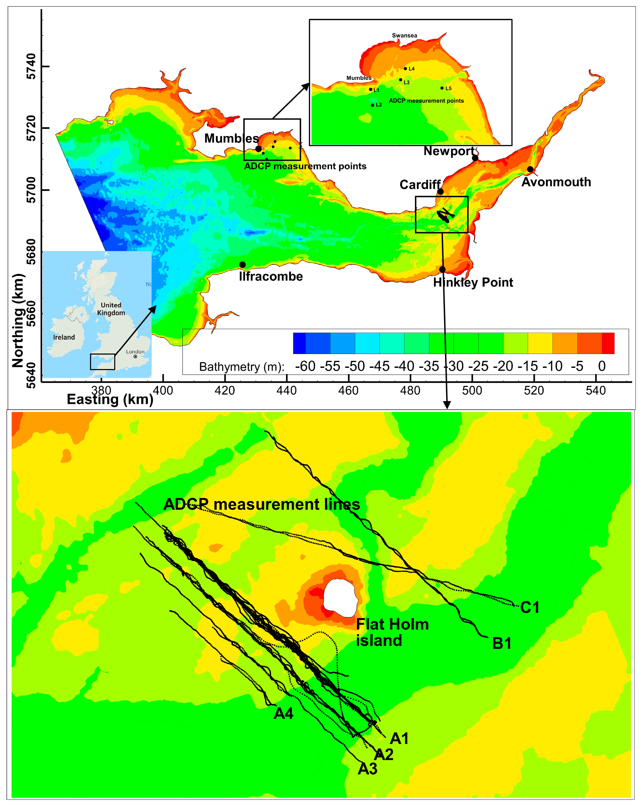
Flat Holm Island lies almost at the boundary of the Severn Estuary and Bristol Channel, approximately 8 km south from Cardiff Bay (Figure 1). It is roughly circular in shape with a diameter of approximately 700 m. Tides in the Severn Estuary are semi-diurnal, with the second largest tidal range in the world [29], with typical tidal ranges during peak spring tides ranging from approximately 7 m at the mouth of Bristol Channel to 14 m in the upper reaches of the Seven Estuary. Maximum currents in this region are approaching excess of 2.5 m/s during peak spring tides [30].
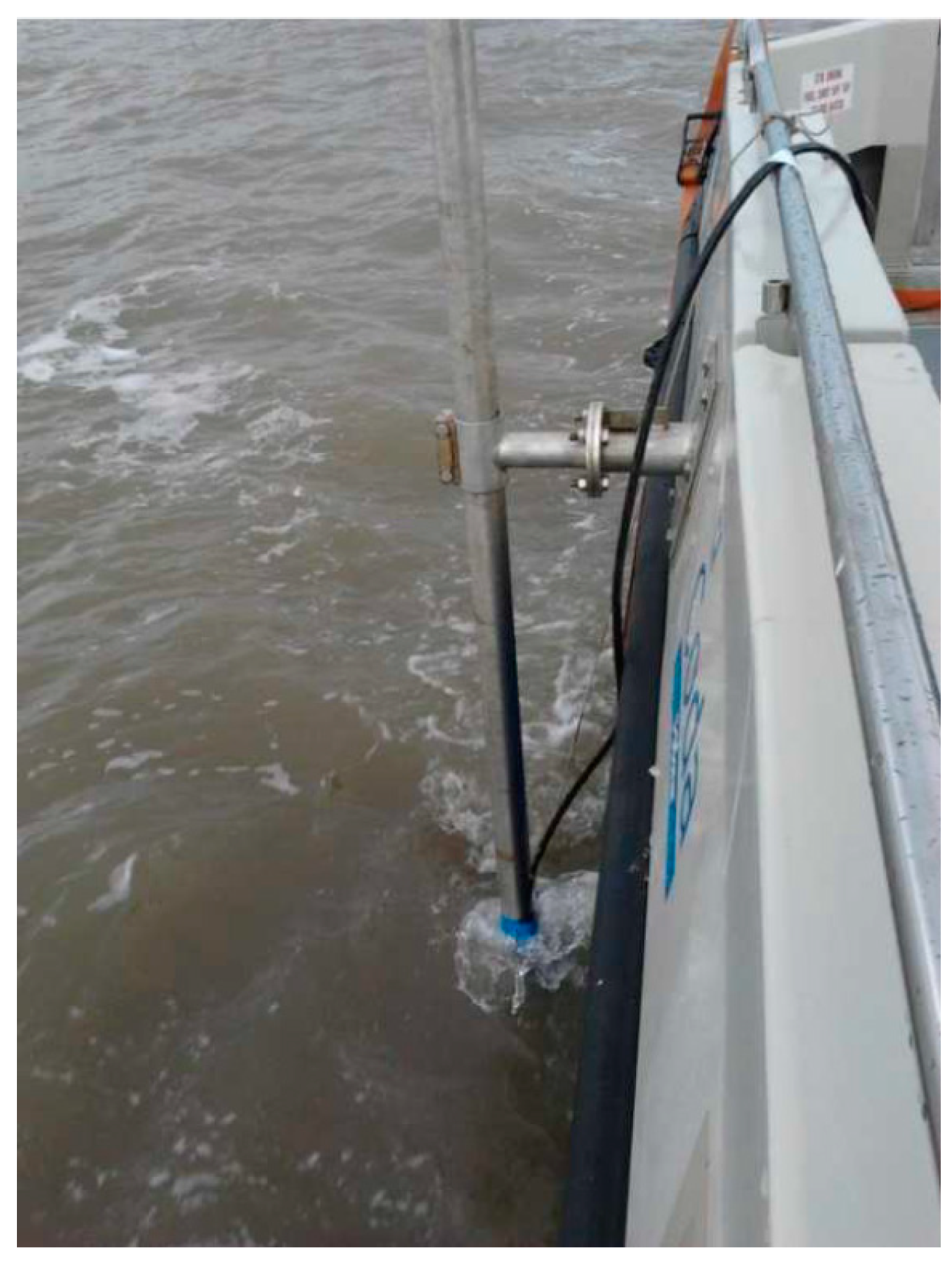
In order to get a better understanding of the flow structure and validate the model performance, vessel-mounted ADCP surveys were carried out in the vicinity of the island between 5 July 2011–30 September 2011 using a Sontek 1000 kHz ADCP. This ADCP unit houses three transducers, measuring the Doppler movement in the east, north, and upward directions. An internal compass and a temperature sensor were also housed within this unit. The Sontek 1000 kHz ADCP was mounted on a swing arm placed at one side of a ship, as demonstrated in Figure 2. Sontek Current Surveyor software was used to record the survey data, which also recorded the vessel position using an onboard Differential Global Positioning System (DGPS). A single beam echo sounder was also employed to provide a profile of the seabed. The vessel transected along a series of survey lines downstream of the island, in as straight a line as possible given the strong tidal current conditions (Figure 1). The survey transects were planned based on the natural features, tidal current conditions, and the potential location of the wake in the lee of the island (Table 1). For example, the survey on 5 July 2011 comprised driving the vessel along a single transect line A1, from the end of the flood tide, throughout the ebb tide and into the beginning of the next flood tide. This ensured that data were acquired to the southwest of Flat Holm, downstream of the ebb tide, and along one transect throughout the ebb tide. The surveying on other days was taken at different tidal phases and locations, with the aim of characterising the flood/ebb tidal currents downstream of Flat Holm Island.
2.2. Modelling System and the Turbulence Models
Telemac-2D is an open-source 2D hydrodynamic module of a hydro-environmental model suite, named TELEMAC. The model was originally developed by EDF R&D (Paris, France) and has been used in a range of applications and by many organisations. Telemac-2D solves the depth-averaged free surface flow equations with second order partial differential equations, using finite elements and a triangular mesh [31]. The governing equations of Telemac-2D, including continuity and momentum along the x and y axes, are provided below for completeness, with further details being given in Hervouet [32].
where h is the depth of water; Z is the free surface elevation; u, v are the depth-averaged velocity components in the x and y directions while u is the vector of velocity; is the turbulent diffusion coefficient; t is time; is the source or sink term of fluid mass, , are the source or sink terms of fluid momentum, representing wind shear, the Coriolis force, and bottom friction within the domain.
Telemac-2D offers four different turbulence modelling schemes. The first method involves using a constant viscosity coefficient that include both molecular viscosity and turbulence viscosity throughout the model domain, with velocity diffusivity value of 10−4 m2/s following the same value of other researchers [33,34].
The second method is the Elder model, which offers the possibility of specifying two different viscosity values for the longitudinal diffusion, i.e., Kl, and the transver diffusion, i.e., Kt. Those two viscosity values are expressed as
where is the shear velocity (or friction velocity), h is the water depth, and and are dimensionless empirical coefficients. Elder has defined and as a constant value of 5.9 and 0.23 separately based on the velocity profile in the logarithmic layer [35]. Fischer et al. [36] further proposed a transverse turbulence diffusion, value of about 0.6 in irregular natural streams with weak meanders. More recently, Wu et al. [37] applied values for αt in the range from 0.6 to 1.0; Steffler and Blackburn [38] set αt to 0.5 with recommended values from 0.2 to 1.0. Different values could be used for and due to the anisotropic features of turbulence structure in the horizontal and vertical directions. For this study, considering the finding of Elder and latter researchers, and are assigned values of 6 and 0.6, respectively, following the advised value of Telemac-2D manual.
The third turbulence model is the classic k-ε model which is based on the calculation of physical quantities representing turbulence in the flow. The eddy viscosity is calculated by
where is an empirical constant and k and ε represent the turbulent kinetic energy and its dissipation rate, respectively, as defined after averaging over the vertical to give
where Zs is the free surface elevation (m), Zf is the bottom elevation (m), is the temporal fluctuation of velocity and the corresponds to the average value of over time.
The k and are determined from the following model transport equations:
where production terms P = , are due to the shear force of flow along the vertical: , , is the dimensionless friction coefficient and is the shear velocity calculated as [39].
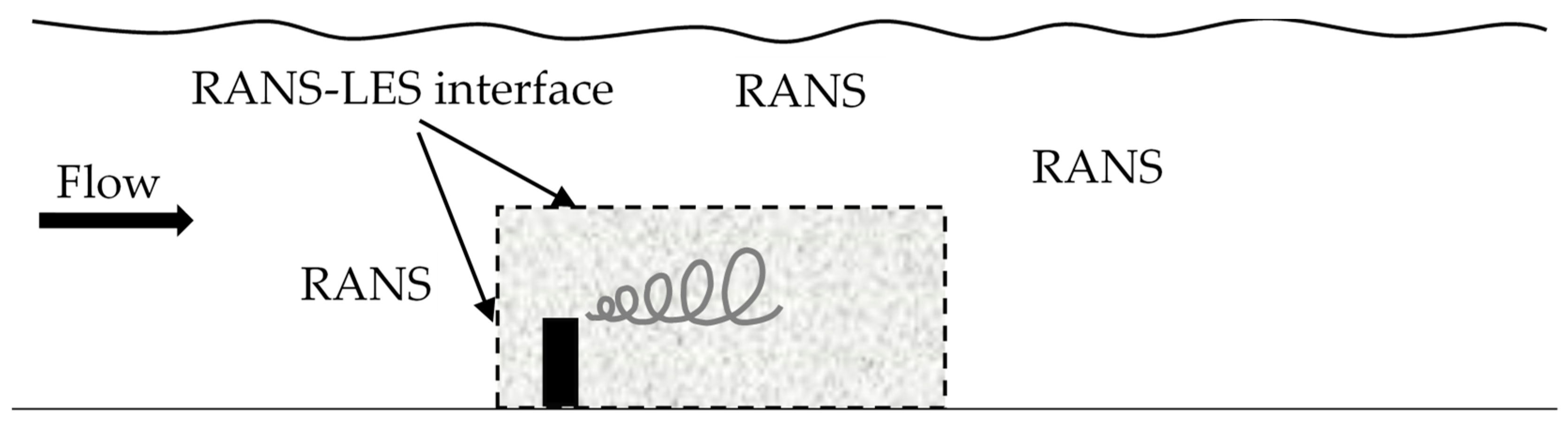
Finally, in modelling the flow around Flat Holm island it would be ideal to embed a Large Eddy Simulation (LES) model within the Reynolds Averaged Navier Stokes (RANS) Telemac-2D model, as illustrated in Figure 3.
However, this was not practical, particularly in terms of the computational resources required for such a large domain, but a Smagorinski model [40] based on the mixing length formulation and including some aspects of Large Eddy Simulation modelling was implemented as a compromise. The principle of the Smagorinski model is to add a turbulent viscosity deduced from a mixing length model to represent the small-scale turbulence. However, since the Smagorinsky model is linked to the grid size in the current study, and with the grid size being 50 m in the vicinity of the island, then sub-grid scale or small-scale turbulence below this grid size is not properly reproduced in this study. Using the Smagorinsky model, the eddy viscosity is calculated from
where is a dimensionless coefficient to be calibrated and is the mesh size. The is the strain rate tensor of average motion, with
For boundary conditions in Telemac-2D, there is no flow flux pass through solid, and for all velocity vectors tangential to a free stream boundary then a free slip condition is applied [41]. The wave equation method, which has been widely used in turbulence studies, was used to solve the continuity and momentum equations in this study [11,32,42]. In this method, the velocity in the continuity equation is substituted from the momentum equation to generate a wave equation, in which the water depth is the only unknown.
Similar spatial discretization is used for all the variables, and, although the equations are expressed in a non-conservative form, the discretization of this method ensures exact conservation of water mass [32].
2.3. Model Setup
The model domain includes the entire Bristol Channel and the Seven Estuary (Figure 1). The open seaward boundary was located at the western extent of the model domain in the outer Bristol Channel, close to Lundy Island, and spanning from from Stackpole Head at the northern limit to Hartland Point at the southern limit. The offshore boundaries were set at outer Bristol Channel which is 115 km away from the island and as far away from the region of interest as practically feasible, to ensure that the approximations at the open boundary (such as normal incoming velocities) did not affect the predictions in the region of interest and the hydrodynamics around the island did not unduly affect the boundary conditions on the ebb tide [43]. A tidal time series of water levels was applied using data obtained from the Proudman Oceanographic Laboratory (POL) Irish Sea model [44]. The Eastern extent of the model was the River Severn tidal limit at Haw Bridge, close to Gloucester. Bathymetric data in this area were obtained from EDINA Digimap, relative to chart datum (CD), with a grid resolution of 30 m. The unconstructed flexible mesh was adopted in this study connecting the Digimap bathymetric data through the following function:
where L is the mesh resolution and X is the bathymetric elevation at that point. Using this setting, the mesh resolution is directly linked to the local depth and gradients, with a finer mesh being used in shallower water and higher gradients and, conversely, a coarser mesh where the water depth is relatively deep and the gradient is low. The area around Flat Holm Island has been refined further to achieve mesh resolution of around 50 m, in order to ensure accurate representation of the bathymetry in this region. The final mesh consists of 286,869 nodes and 570,156 triangular cells. To ensure the model accuracy, the Courant number limitation was set to 1, and a time step of 10 s was set to meet the Courant-Friedrichs-Lewy (CFL) limit.
L = −6.5 X + 200
2.4. Analysis Tools
The model was calibrated and validated against water levels and current speed and direction. The Coefficient of Determination (R2) and the Root Mean Squared Error (RMSE) were used to assess model performance as follows:
where are the observed values, are the mean of the observed values, are the predicted values, are the mean of the predicted values. Maréchal [45] used R2 to assess model performance, namely excellent (R2 > 0.85), very good (0.65 < R2 < 0.85), good (0.5< R2 < 0.65), and poor (0.2 < R2 < 0.5). However, the RMSE value is mainly relevant to scalar quantities, not vector quantities. In this case, the Mean Absolute Error (MAE) was used. The MAE includes errors of both magnitude and direction in a single statistic. For a 2D vector ,
The performance of the model could also be judged from the value of the Relative Mean Absolute Error (RMAE). An RMAE value of zero implies a perfect match between predictions and observations:
The preliminary qualification for RMAE ranges suggested by Walstra [46], that is Excellent (RMAE < 0.2), Good (0.2 < RMAE < 0.4), Reaonable (0.4 < RMAE < 0.7), Poor (0.7 < RMAE < 1.0), Bad (RMAE > 1.0).
3. Results and Discussion
3.1. Model Calibration and Validation
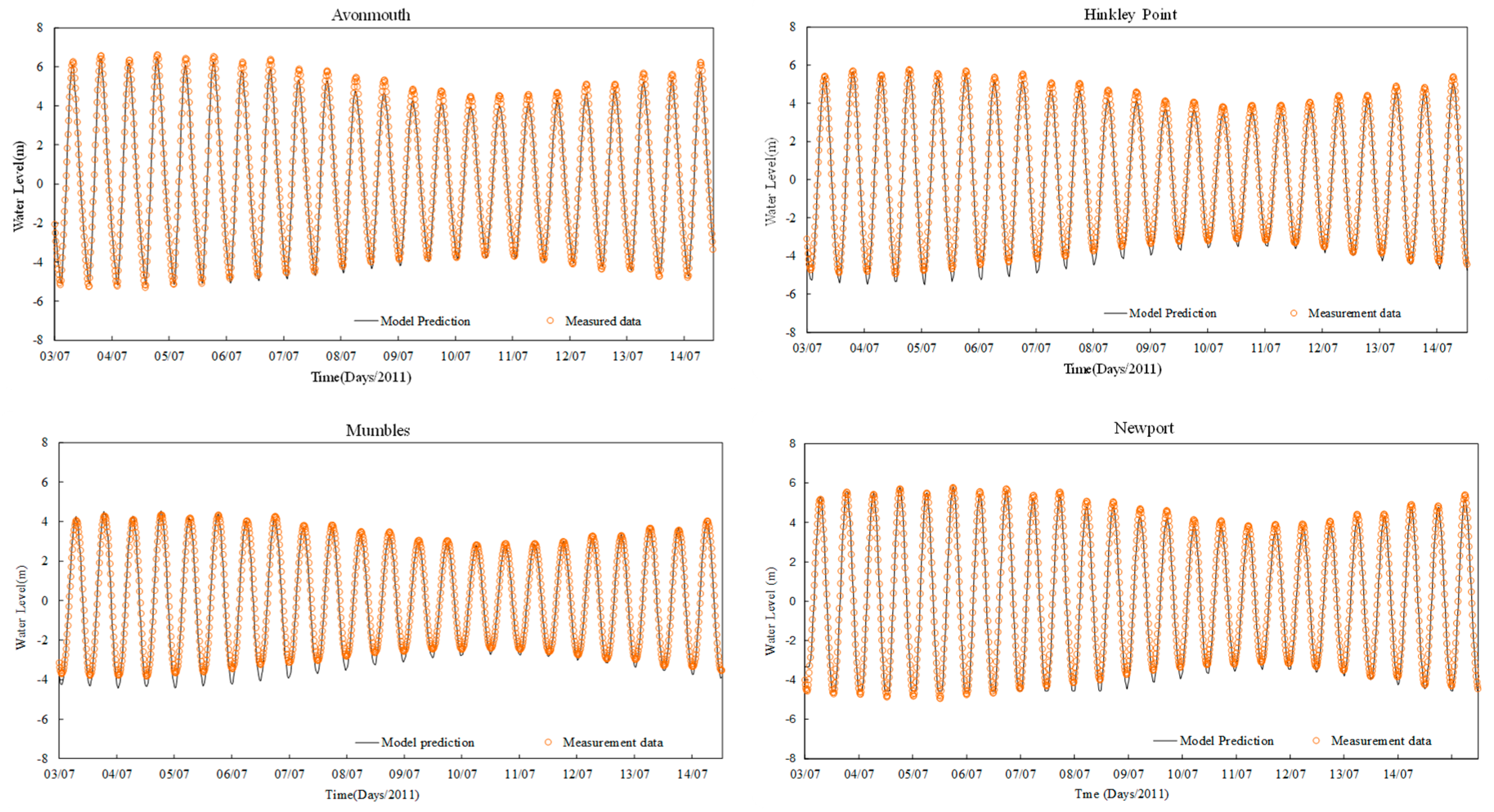
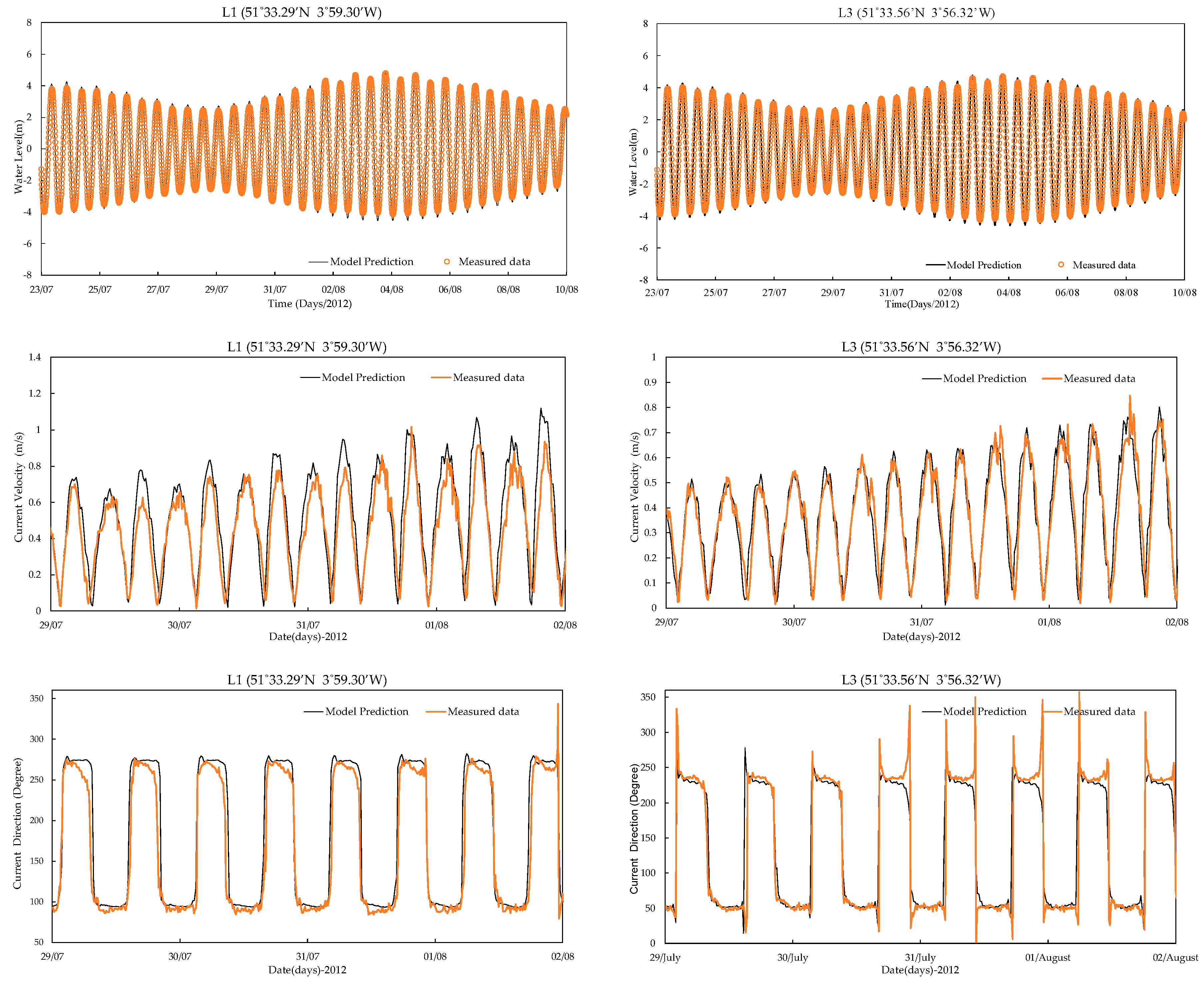
The model performance was validated using water levels at four tidal gauge sites across the modelling domain. Water levels at these sites were acquired from British Oceanographic Data Centre (BODC) tidal gauges (Figure 1). The validation period was from 2 July 2011 to 15 July 2011 due to the availability of current data. Model predictions and measured values at these sites are compared (Figure 4), while a statistical analysis of the model performance is carried out (Table 2). From this part of the calibration results, the coefficient of determination (R2) shows a strong correlation between the modelled and observed data, and RMSE value is also encouraging bearing in mind the high tidal range and currents. However, validation data of model against the Newport gauges show relatively poor agreement. This was believed to be due to the inconsistencies in the bathymetric data in this region. The hydrodynamic performance of the model was further validated against data collected using five bed-mounted ADCPs deployed in Swansea Bay between September 2012 and December 2012. The current speeds and velocities were measured throughout the water depth at these sites using seabed mounted ADCPs (Figure 1). The corresponding field data were then integrated over depth to acquire the depth average values. Typical comparisons between the model predictions and measured data for water levels and current speeds and directions and a summary of the statistical analysis are given (Figure 5, Table 2). The statistic values all show good correlation. For water level, all R2 are higher than 0.99 and RMSE is relatively small. For velocity validation, three RMAE locate in ‘excellent’ and two are ‘very good’. In summary, validation of the model shows very good correlation between the model predictions and measured field data and, therefore, the model verification is considered acceptable and appropriate for examining the flow around Flat Holm Island.
Tidal constituents were also compared to conduct a further model validation test. The model was run for more than 30 days, from 18 January 2012 to 19 February 2012, to achieve an accurate harmonic analysis; Matlab package T-tide [47] was utilized to determine the harmonic constituents, with the top three dominant constituents being the M2, S2, and N2 tides. Tidal BODC measurement data and model predictions were compared at the tidal gauges in the Bristol Channel (Table 3).
Results show that the amplitude and phase for the M2, S2 and N2 tidal constituents match very well, with most having a difference of less than 5%. While the M2 phase shows a discrepancy at the Newport site of close to 10%, which could be experiencing some impact from the River Usk and the complex and relatively shallow bathymetry.
3.2. Comparison of Turbulence Schemes
Modelling turbulence accurately in the region of interest is challenging due to the rapid transformation of the tidal flow and the complex turbulence-generating bathymetric features. Various methodologies using different levels of complexity can be used to simulate the turbulence levels and structure observed in the field. Four different turbulence schemes are included in Telemac-2D, and they were all assessed to identify the most appropriate scheme to simulate wakes in the lee of islands in a macro-tidal estuary. In order to compare the behaviour of different turbulence models, four Telemac-2D models with different turbulence models have been compared. The MAE and RMAE parameters have been calculated by comparing the measured ADCP data and the prediction data to give the averaged values (Table 4). The results highlight the impact of the different turbulence models on the hydrodynamic model performance. Generally, the RMAE are all smaller than 0.4, which in reference to the Qualification of RMAE (In Section 2.4) this means that all the prediction data with turbulence models have a ‘good’ correlation with measured data and therefore are suitable for predicting the flow patterns in the wake of an island in a macro-tidal estuary. However, the k- model showed the smallest MAE and RMAE, which indicates that is the most accurate turbulence model in this case.
3.3. Comparison of Different k-ε Solvers
Emphasis was then focused on studying the k- model for simulating the wake behind Flat Holm Island. The turbulence model equations were solved by the fractional step method, with advection of the turbulence variables: k (turbulent energy) and ε (turbulent dissipation) being processed at the same time as the hydrodynamic variables, and the other terms relating to the diffusion and production/dissipation of the turbulent parameters being processed in a single step.
The solver used for simulations in the turbulence model has several different options (Table 5). The key solvers include the conjugate gradient method and its derivation method and the generalised minimum residual method (GMRES). The conjugate gradient method is the most prominent iterative method for solving sparse systems of linear equations [48]. It is an algorithm for finding the nearest local minimum of a function of n variables, which presupposes that the gradient of the function can be computed. The GMRES method is especially useful for poor conditional system.
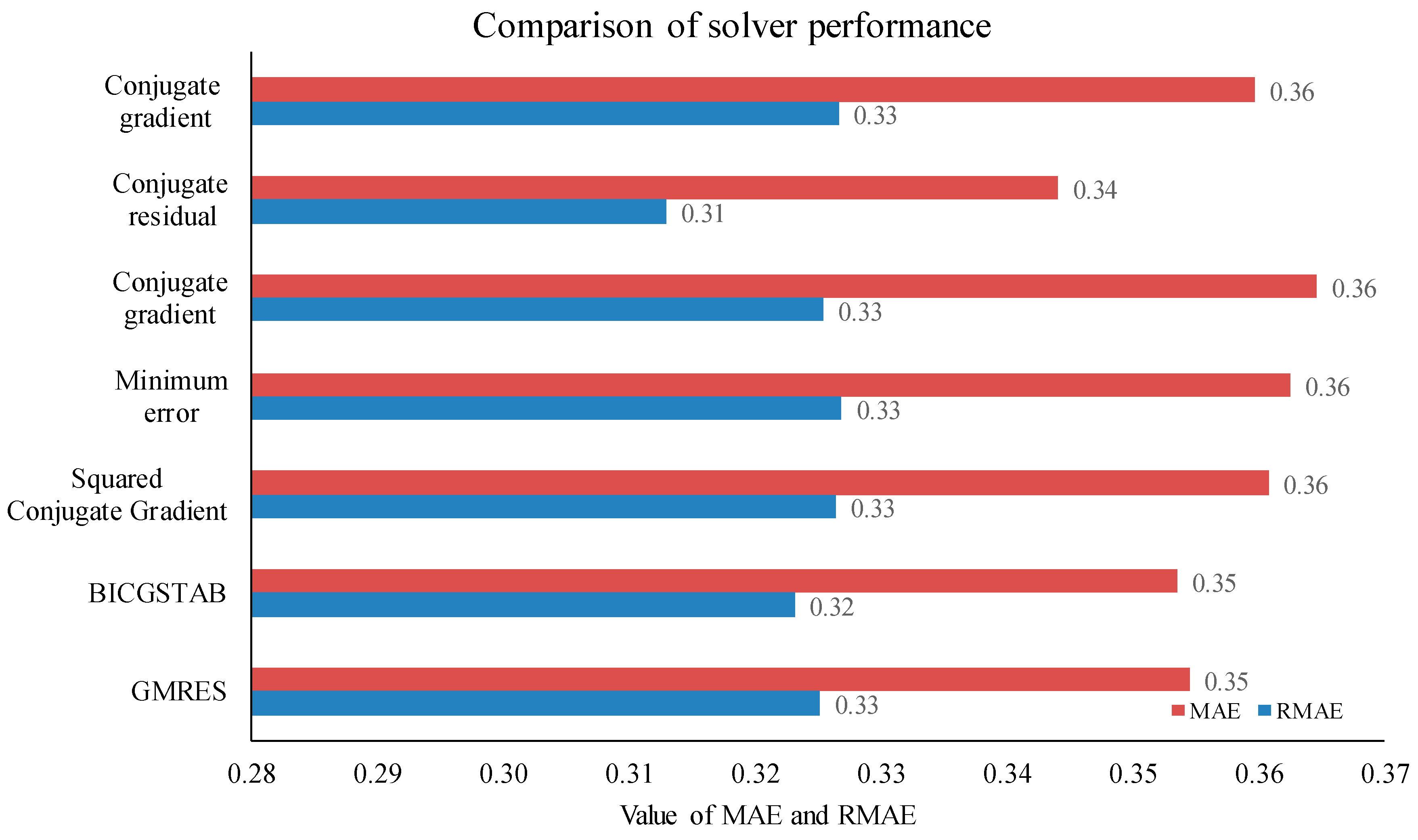
The performances of each solver in predicting the wake behind the island are summarized (Figure 6 and Table 5). All k-ε solvers showed good results, while the conjugate residual showed the smallest MAE and RMAE and subsequently the slightly better performance in simulating the wake flows in the lee of Flat Holm island. Therefore, the conjugate residual solver was used throughout the remainder of this study.
3.4. Model Comparison with ADCP Data
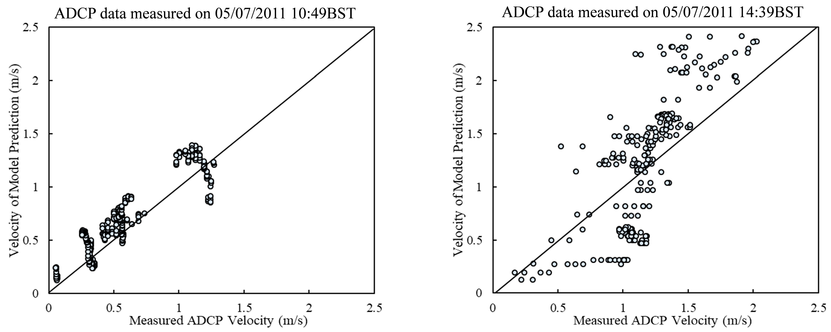
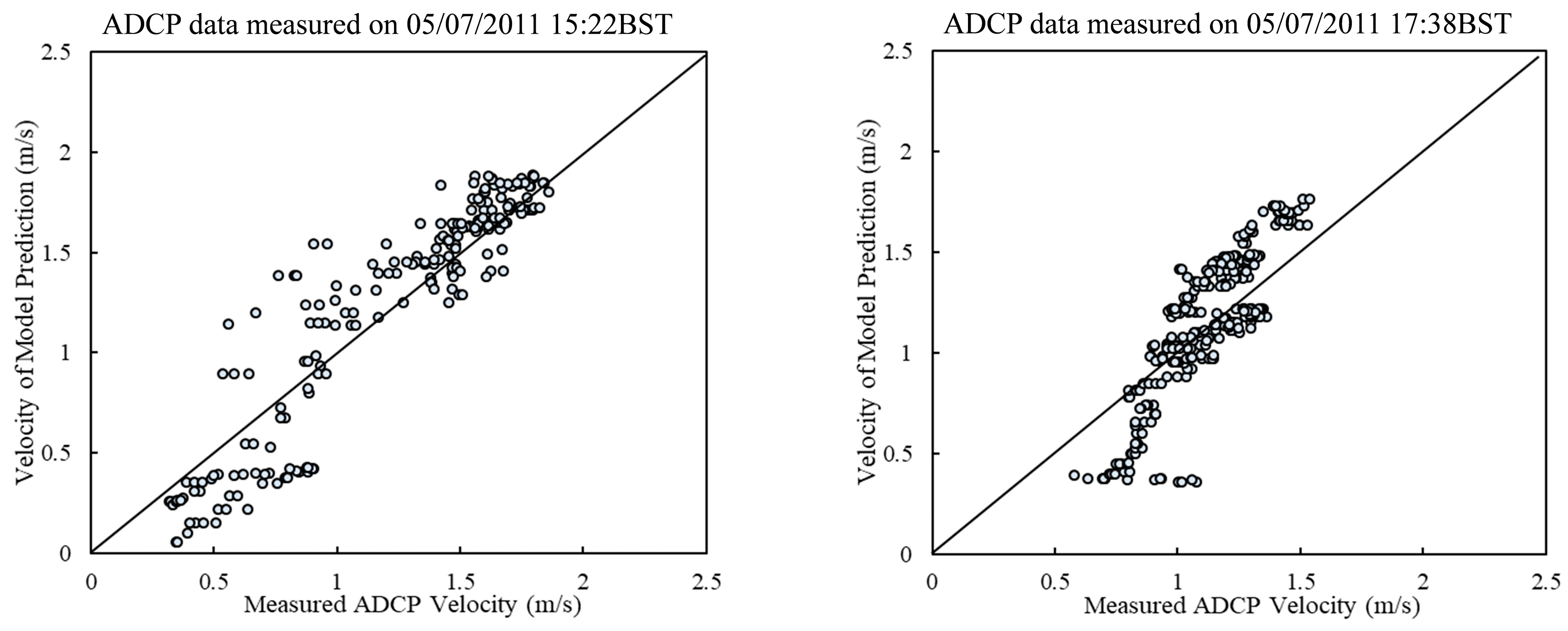
The measured and predicted velocity magnitude along these four transects are compared by scatter plots of gene expression (Figure 7). The values of the velocities predicted from the model at various points are shown along the Y axis, while the X axis represents the measured velocity values at these same points. This demonstrates the variability in the model performance, which is linked to the location of the measured points. For example, for the ADCP data collected on 5 July 2011 at 10:49, the model behaves well in the low-velocity zone, which corresponds to the recirculation zone in the lee of the island. This indicates that the model simulates the island wake well. On the other hand, the model results show a weaker performance in the high-velocity zones, which are on the two sides of the island to the south east of the island and where the deep trench is located. The results generally show good correlation between the measured data and the model predictions.
3.5. The Evolution of Wake in the Lee of Island
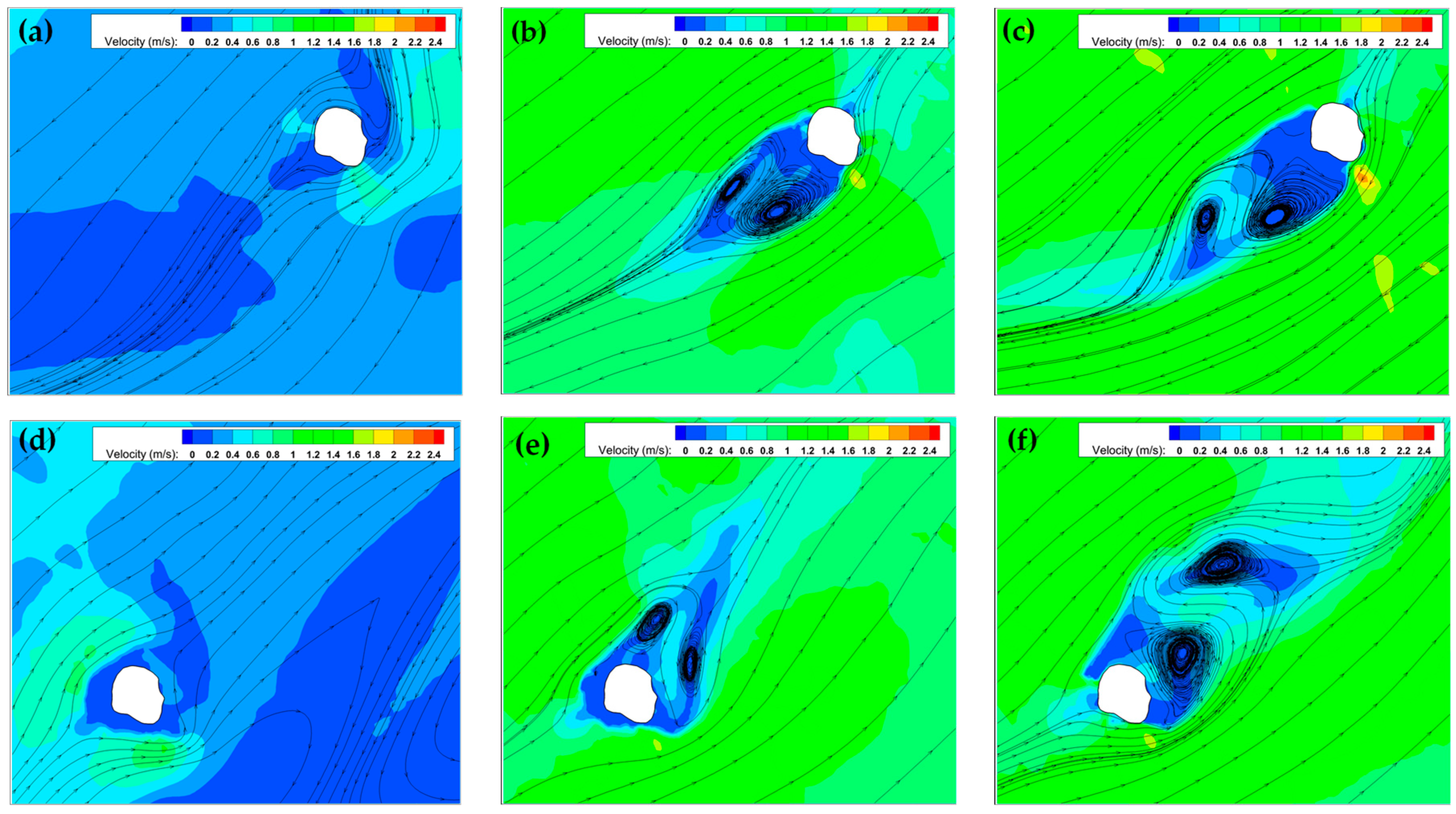
The evolution of wake during the neap tide on 11 July 2011 are shown in Figure 8. It can be seen that the evolution of wake has the similar trend during the ebb and flood tide. First, when it is the slack tide condition (high water level or low water level), low velocity tidal currents resulting in steady flow around Flat Holm island, and with no vortex being generated (Figure 8a,d). With the increase of the tide velocity, two vortices were generated at the same time, with relative steady side-by-side position and no eddy shedding occurring (Figure 8b,e). Around the peak velocity of neap tide (Figure 8c,f), typical Karman vortex street appears in the wake. Figure 8 shows a similar trend in the developing wake during flood tide and ebb tide, and during neap tides. Thus, model predictions show that the same wake pattern is generated under the same tidal currents despite the different water depths. However, this phenomenon does not directly mean that the wake developing in the lee of Flat Holm is not related to with the water depth. First, the change in the water depth change is relatively slow during neap tides. Second, the bathymetry to the west-south of Flat Holm island is higher than that to the north-east side, as shown in Figure 1. This difference in the bathymetry results in slightly higher tide speeds upstream of the island (i.e., on the south-west side) during flood tides when compared with the tidal velocity upstream of the island (i.e., on the north-east side) during ebb tides. These reasons combine to account for the same wake evolution being developed during the flood and ebb neap tides.
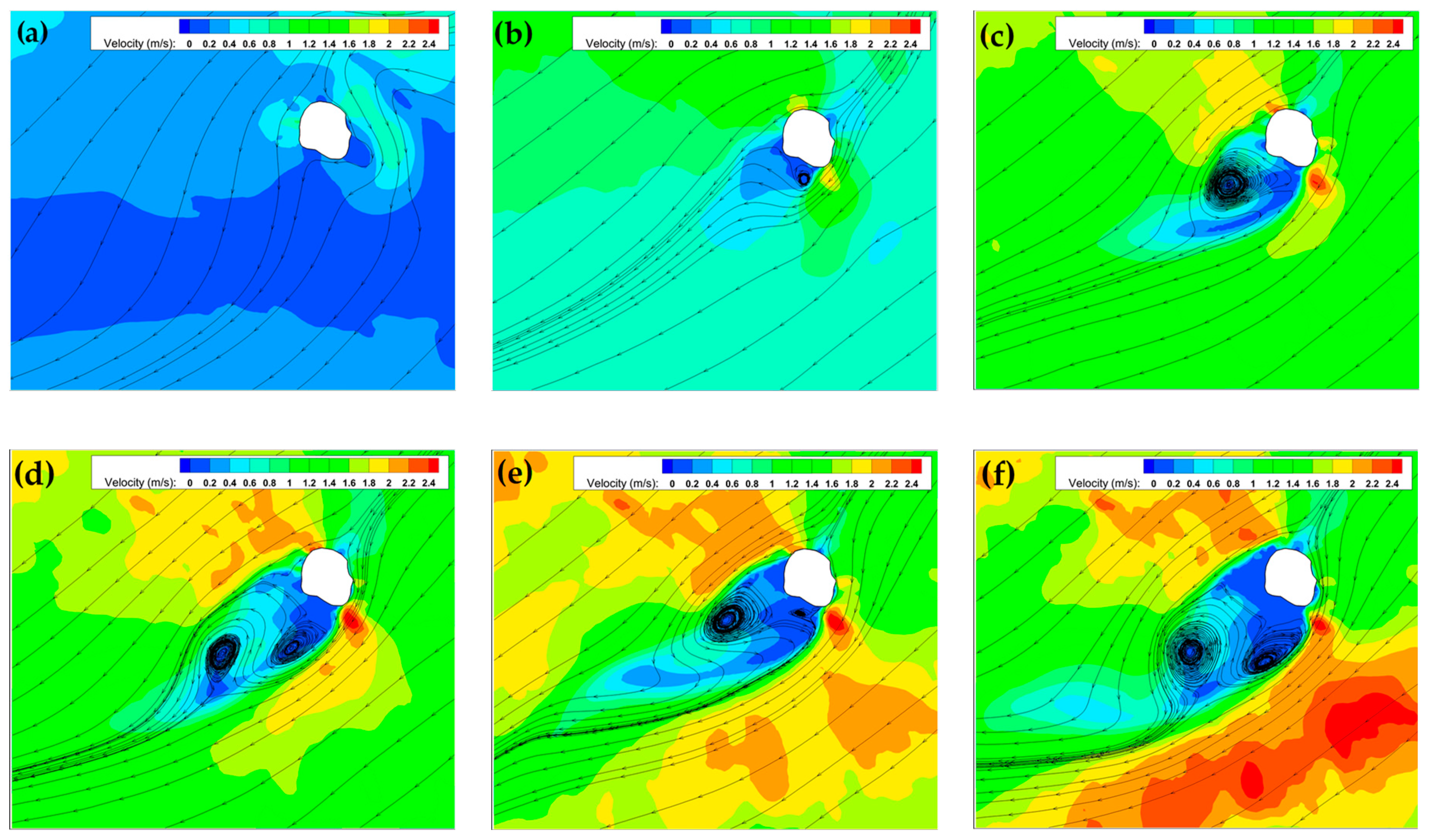
To compare the difference in the developing wake between neap and spring tides, an analysis for the wake developing during the spring tide has been undertaken for 5 July 2011 and for a shorter time interval, as shown in Figure 9 and Figure 10. At the beginning of the ebb spring tide (i.e., Figure 9a), no vortex is present in the lee of the island for the relatively low tidal velocities. With an increase in the tidal velocity and a decrease in the water depth, a tidal eddy is generated, which grows in size, as shown in Figure 9b,c and with no eddy shedding occurring. The island wake keeps developing, leading to an unsteady Karman Vortex Street, see Figure 9d–f.
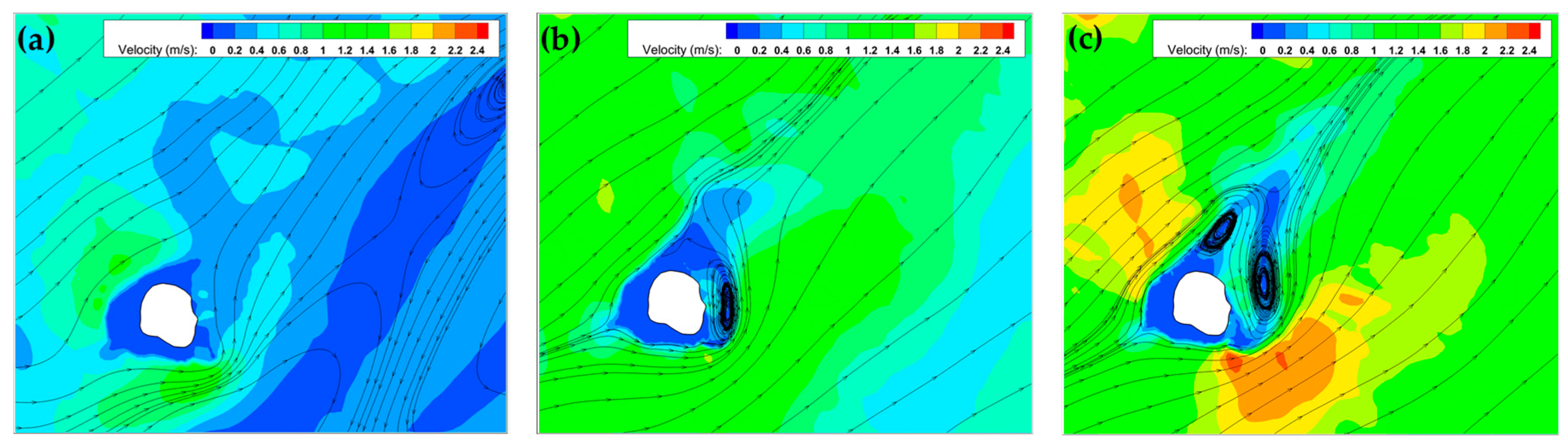
The wake during the flood phase is somewhat different to the ebb phase, probably due to the higher velocity along with the relatively shallow bathymetry to the south-western side of Flat Holm Island, which can be observed in Figure 1. The early stages of wake development during the flood tide is similar to the ebb. One vortex is generated, its size increasing with increasing velocity and water depth (Figure 10b) before a steady wake with two vortices are generated, no eddy shedding occurring. These two vortices are generally stable with very little migration or increase in size.
The Reynolds number (Re) has been commonly used to describe the characteristics of island wakes, especially in experimental studies, because Re is based on the kinematic viscosity of the fluid and frictional boundary layers, which are generated in the laboratory by friction and boundary layer separation [49]. However, in real environmental flows, it is the turbulent viscosity which dominates the wake development [50]; therefore, Re is not suitable to quantify the characteristics of wakes since Re is based on the kinematic viscosity of the fluid. Subsequently, the wake behind an island in reality is often described by the island wake parameter [13], namely,
where U0 is the free stream velocity, D is the water depth, L is the diameter of island, and Kz is the vertical eddy diffusion coefficient. When P << 1, friction is dominant and quasi-potential flow results. A relatively stable wake is present when P ≈ 1. For P >> 1, then bottom friction effects are weak, and an unsteady wake is formed, similar to the flow around obstacles at a large Re value in laboratory experiments. For Flat Holm island, the island diameter (L) is about 700 m and kept constant during the rise and fall of tide due to its steep cliff. While the vertical eddy viscosity (Kz) in the Bristol Channel is defined as 0.20 m2 s−1 [50,51]. The free stream velocity U0 and water depth are taken at 400 m upstream away from Flat Holm Island. The island wake parameter (P) corresponding to different tide condition are calculated (Table 6).
The island wake parameter of HW and HW + 0.5 h are 0.79 h and 0.86 h, respectively, which is between P << 1 and P ≈ 1. This is related to the early stages of wake generation before transforming into a stable wake, which meets the vortex generation process shown in Figure 9a–c matches the description of P ≈ 1, the stable condition. With the increase of P, the wake gradually transforms into an unsteady condition, as illustrated in Figure 9e,f.
Figure 10 also shows a good correlation to the island wake parameter, with the exception of the early stages of a flood tide (Figure 10a) where no wake is generated. Other figures all show a stable wake, with either one vortex or two vortices (Figure 10b–f). The corresponding P varies between 0.42–1.2. Although the P for LW + 0.5 h and LW + 1 h have a relatively low value, the overall revolution of wake meets the prediction of P.
These results demonstrate that the island wake parameter was capable of informing on the wake behaviour in the lee of an island located in a macrotidal environment and could be considered for simulating wakes behind obstacles in similar estuarine and coastal environments.
4. Summary and Conclusions
The wake developed in the lee of an island in a macrotidal estuary, namely Flat Holm Island, located in Severn Estuary and Bristol channel, was studied using a 2D finite element model (Telemac-2D), with field measurements also acquired for model validation. The numerical model was set-up to cover the entire Severn Estuary and Bristol Channel, covering an area of 5793 km2. The general performance of the model was first validated against water levels and velocities measured across the domain. Further field surveys were undertaken with vessel-mounted ADCP data being acquired specifically around the island and for different tidal conditions to validate and improve the models predictions. To acquire better model predictions, four different turbulence model were tested and compared, including: a constant eddy viscosity model, an Elder model, a k-ε model, and a Smagorinski LES-based model. The k-ε model showed the best performance when compared with the field measurements and was chosen for this study. Furthermore, six different methods to solve the k-ε model equation were considered and compared. All models showed good predictions compared to the field measurements around the island, while the best results were acquired by using the conjugate residual. The conjugate residual solver was selected and then used in this study.
The simulation results show that the wake development is symmetrical at two sides of island in the neap tide, that two steady vortices appear in the wake with the increase of the tide velocity, changing into stable Karman vortex street around the peak tide moment. The vortex generated in the wake of Flat Holm Island were studied using the island wake parameters. Based on the definition of this parameter, a stable wake was expected during flood tides while unsteady wakes were expected during ebb tides. These findings were confirmed through the presence of the stable eddies during flood tides and an unsteady vortex street was observed during ebb tides. The results confirm the applicability of the island wake parameter in predicting wake behaviour behind an island located in a macro-tidal estuarine environment; therefore, similar approaches could be considered for simulating wakes behind obstacles in similar estuarine and coastal environments.
Author Contributions
B.G. carried out the research, including: setting up the Telemac-2D model, analysing the development of the island wake and drafting the manuscript. R.A. proposed and supervised the research. P.E. provided the vessel-mounted ADCP data and reviewed the manuscript. R.A.F. reviewed the manuscript. All authors have read and agreed to the published version of the manuscript.
Funding
This research received no external funding.
Acknowledgments
The authors would like to express their gratitude to Chris Wooldridge for the leading the in situ data collection studies and acknowledge the support of the Chinese Scholarship Council (CSC) and Cardiff University for this PhD study and would like to thank them for their support. The first author also acknowledges the support through the National Key R&D Program of China (Grant No.: 2018YFB1501901).
Conflicts of Interest
The authors declare no conflict of interest.
References
- Evans, P.; Lazarus, E.D.; Mason-Jones, A.; O’Doherty, D.M.; O’Doherty, T. Wake characteristics of a natural submerged pinnacle and implications for tidal stream turbine installations. In Proceedings of the 11th European Wave and Tidal Energy Conference, Nantes, France, 6–11 September 2015. [Google Scholar]
- Estrade, P.; Middleton, J.H. A numerical study of island wake generated by an elliptical tidal flow. Cont. Shelf Res. 2010, 30, 1120–1135. [Google Scholar] [CrossRef]
- Hamner, W.M.; Hauri, I.R. Effects of island mass: Water flow and plankton pattern around a reef in the great barrier reef lagoon, Australia. Limnol. Oceanogr. 1981, 26, 1084–1102. [Google Scholar] [CrossRef]
- Pingree, R. The formation of the shambles and other banks by tidal stirring of the seas. J. Mar. Biol. Assoc. UK 1978, 58, 211–226. [Google Scholar] [CrossRef] [Green Version]
- Dyer, K.R.; Huntley, D.A. The origin, classification and modelling of sand banks and ridges. Cont. Shelf Res. 1999, 19, 1285–1330. [Google Scholar] [CrossRef]
- Neill, S.P.; Scourse, J.D. The formation of headland/island sandbanks. Cont. Shelf Res. 2009, 29, 2167–2177. [Google Scholar] [CrossRef]
- Li, Y.; Song, Z.; Peng, G.; Fang, X.; Li, R.; Chen, P.; Hong, H. Modeling Hydrodynamics in a harbor area in the Daishan Island, china. Water 2019, 11, 192. [Google Scholar] [CrossRef] [Green Version]
- Gou, H.; Luo, F.; Li, R.; Dong, X.; Zhang, Y. Modeling study on the hydrodynamic environmental impact caused by the sea for regional construction near the Yanwo Island in Zhoushan, China. Water 2019, 11, 1674. [Google Scholar] [CrossRef] [Green Version]
- Neill, S.P.; Jordan, J.R.; Couch, S.J. Impact of tidal energy converter (TEC) arrays on the dynamics of headland sand banks. Renew. Energy 2012, 37, 387–397. [Google Scholar] [CrossRef]
- Finkl, C.W.; Charlier, R. Electrical power generation from ocean currents in the straits of Florida: Some environmental considerations. Renew. Sustain. Energy Rev. 2009, 13, 2597–2604. [Google Scholar] [CrossRef]
- Stansby, P.; Chini, N.; Lloyd, P. Oscillatory flows around a headland by 3d modelling with hydrostatic pressure and implicit bed shear stress comparing with experiment and depth-averaged modelling. Coast Eng. 2016, 116, 1–14. [Google Scholar] [CrossRef]
- Dewey, R.; Richmond, D.; Garrett, C. Stratified tidal flow over a bump. J. Phys. Oceanogr. 2005, 35, 1911–1927. [Google Scholar] [CrossRef]
- Wolanski, E.; Imberger, J.; Heron, M.L. Island wakes in shallow coastal waters. J. Geophys. Res. 1984, 89, 10553–10569. [Google Scholar] [CrossRef]
- Lacey, R.J.; Rennie, C.D. Laboratory investigation of turbulent flow structure around a bed-mounted cube at multiple flow stages. J. Hydraul. Eng. 2011, 138, 71–84. [Google Scholar] [CrossRef]
- Arbic, B.K.; Richman, J.G.; Shriver, J.F.; Timko, P.G.; Metzger, E.J.; Wallcraft, A.J. Global modeling of internal tides: Within an eddying ocean general circulation model. Oceanography 2012, 25, 20–29. [Google Scholar] [CrossRef] [Green Version]
- Blaise, S.; Deleersnijder, E.; White, L.; Remacle, J.-F. Influence of the turbulence closure scheme on the finite-element simulation of the upwelling in the wake of a shallow-water island. Cont. Shelf Res. 2007, 27, 2329–2345. [Google Scholar] [CrossRef]
- Pattiaratchi, C.; James, A.; Collins, M. Island wakes and headland eddies: A comparison between remotely sensed data and laboratory experiments. J. Geophys. Res. 1987, 92, 783–794. [Google Scholar] [CrossRef]
- Coutisa, P.F.; Middleton, J.H. The physical and biological impact of a small island wake in the deep ocean. Deep Sea Res. Part I 2002, 49, 1341–1361. [Google Scholar] [CrossRef]
- Neill, S.P.; Elliott, A.J. In situ measurements of spring–neap variations to unsteady island wake development in the firth of forth, Scotland. Estuar. Coast. Shelf Sci. 2004, 60, 229–239. [Google Scholar] [CrossRef]
- Williams, R.D.; Brasington, J.; Hicks, M.; Measures, R.; Rennie, C.D.; Vericat, D. Hydraulic validation of two-dimensional simulations of braided river flow with spatially continuous aDcp data. Water Resour. Res. 2013, 49, 5183–5205. [Google Scholar] [CrossRef] [Green Version]
- Ahmadian, R.; Olbert, A.I.; Hartnett, M.; Falconer, R.A. Sea level rise in the severn estuary and bristol channel and impacts of a severn barrage. Comput. Geosci. 2014, 66, 94–105. [Google Scholar] [CrossRef]
- Dastgheib, A.; Roelvink, J.; Wang, Z. Long-term process-based morphological modeling of the Marsdiep tidal basin. Mar. Geol. 2008, 256, 90–100. [Google Scholar] [CrossRef]
- Jones, J.E.; Davies, A.M. Storm surge computations for the west coast of britain using a finite element model (TELEMAC). Ocean Dyn. 2008, 58, 337–363. [Google Scholar] [CrossRef] [Green Version]
- Falconer, R.A.; Wolanski, E.; Mardapitta-Hadjipandeli, L. Modeling tidal circulation in an island’s wake. J. Waterw. Port Coast. Ocean Eng. 1986, 112, 234–254. [Google Scholar] [CrossRef]
- Draper, S.; Borthwick, A.G.; Houlsby, G.T. Energy potential of a tidal fence deployed near a coastal headland. Philos. Trans. A Math. Phys. Eng. Sci. 2013, 371, 20120176. [Google Scholar] [CrossRef] [PubMed] [Green Version]
- Falconer, R.A.; Xia, J.; Lin, B.; Ahmadian, R. The Severn Barrage and other tidal energy options: Hydrodynamic and power output modeling. Sci. China Ser. E 2009, 52, 3413–3424. [Google Scholar] [CrossRef]
- Neill, S.P.; Angeloudis, A.; Robins, P.E.; Walkington, I.; Ward, S.L.; Masters, I.; Lewis, M.J.; Piano, M.; Avdis, A.; Piggott, M.D.; et al. Tidal range energy resource and optimization—Past perspectives and future challenges. Renew. Energy 2018, 127, 763–778. [Google Scholar] [CrossRef]
- Angeloudis, A.; Falconer, R.A.; Bray, S.; Ahmadian, R. Representation and operation of tidal energy impoundments in a coastal hydrodynamic model. Renew. Energy 2016, 99, 1103–1115. [Google Scholar] [CrossRef] [Green Version]
- Čož, N.; Ahmadian, R.; Falconer, R.A. Implementation of a full momentum conservative approach in modelling flow through tidal structures. Water 2019, 11, 1917. [Google Scholar] [CrossRef] [Green Version]
- Ahmadian, R.; Falconer, R.A.; Bockelmann-Evans, B. Comparison of hydro-environmental impacts for ebb-only and two-way generation for a severn barrage. Comput. Geosci. 2014, 71, 11–19. [Google Scholar] [CrossRef]
- Galland, J.C.; Goutal, N.; Hervouet, J.M. Telemac: A new numerical model for solving shallow water equations. Adv. Water Resour. 1991, 14, 138–148. [Google Scholar] [CrossRef]
- Hervouet, J.M. Hydrodynamics of Free Surface Flows: Modelling with the Finite Element Method, 1st ed.; John Wiley and Sons: Hoboken, NJ, USA, 2007. [Google Scholar]
- Matta, E. Multi-dimensional Flow and Transport Modeling of a Surface Water Body in a Semi-Arid Area. Ph.D. Thesis, Technische Universität Berlin, Berlin, Germany, 2018. [Google Scholar]
- Jourieh, A. Multi-dimensional Numerical Simulation of Hydrodynamics and Transport Processes in Surface Water Systems in Berlin. Ph.D. Thesis, Technische Universität Berlin, Berlin, Germany, 2013. [Google Scholar]
- Elder, J. The dispersion of marked fluid in turbulent shear flow. J. Fluid Mech. 1959, 5, 544–560. [Google Scholar] [CrossRef]
- Fischer, H.B.; List, J.E.; Koh, R.C.Y.; Imberger, J.; Brooks, N.H. Mixing in Inland and Coastal Waters, 1st ed.; Academic Press: San Diego, CA, USA, 1979. [Google Scholar]
- Wu, W.; Wang, P.; Chiba, N. Comparison of five depth-averaged 2D turbulence models for river flows. Arch. Hydro-Eng. Environ. Mech. 2004, 51, 183–200. [Google Scholar]
- Steffler, P.; Blackburn, J. Two-dimensional depth averaged model of river hydrodynamics and fish habitat. In River2D User’s Manual; University of Alberta: Edmonton, AB, Canada, 2002; Available online: http://www.river2d.ualberta.ca/Downloads/documentation/River2D.pdf (accessed on 5 January 2020).
- Rastogi, A.K.; Rodi, W. Predictions of heat and mass transfer in open channels. J. Hydraul. Div. 1978, 104, 397–420. [Google Scholar]
- Rodi, W.; Constantinescu, G.; Stoesser, T. Large-eddy Simulation in Hydraulics; CRC Press: London, UK, 2013. [Google Scholar]
- Martins, F.A.B.D.C.; Fernandes, E.H. Hydrodynamic model intercomparison for the Patos Lagoon (Brazil). In Proceedings of EMS 2004 IASTED Org; Ubertini, L., Ed.; ACTA Press: Calgary, AB, Canada, 2008; pp. 123–126. [Google Scholar]
- Abu-Bakar, A.; Ahmadian, R.; Falconer, R.A. Modelling the transport and decay processes of microbial tracers in a macro-tidal estuary. Water Res. 2017, 123, 802–824. [Google Scholar] [CrossRef]
- Ji, Z.-G. Hydrodynamics and Water Quality: Modeling Rivers, Lakes, and Estuaries, 1st ed.; John Wiley & Sons: Hoboken, NJ, USA, 2017; p. 574. [Google Scholar]
- POL. Continental Shelf Model: Fine Grid(CS3 and CS3-3D). 2011. Available online: https://noc-innovations.co.uk/ocean-innovations/sites/ocean-innovations/files/documents/model-info-CS3.pdf (accessed on 5 January 2020).
- Maréchal, D. A Soil-Based Approach to Rainfall-Runoff Modelling in Ungauged Catchments for England and Wales. Ph.D. Thesis, Cranfield University, Silsoe, UK, 2004. Available online: https://dspace.lib.cranfield.ac.uk/handle/1826/915 (accessed on 2 January 2020).
- Walstra, D.; Van Rijn, L.; Blogg, H.; Van Ormondt, M. Evaluation of a hydrodynamic area model based on the COAST3D data at Teignmouth 1999. In Proceedings of the Coastal Dynamics 2001 Conference, Lund, Sweden, 11–15 June 2001. [Google Scholar]
- Pawlowicz, R.; Beardsley, B.; Lentz, S. Classical tidal harmonic analysis including error estimates in MATLAB using T_TIDE. Comput. Geosci. UK 2002, 28, 929–937. [Google Scholar] [CrossRef]
- Shewchuk, J.R. An Introduction to the Conjugate Gradient Method without the Agonizing Pain; Techical Report; School of Computer Science, Carnegie Mellon University: Pittsburgh, PA, USA, 1994. [Google Scholar]
- Tomczak, M. Island wakes in deep and shallow water. J. Geophys. Res. Oceans 1988, 93, 5153–5154. [Google Scholar] [CrossRef]
- Neill, S.P.; Elliott, A.J. Observations and simulations of an unsteady island wake in the Firth of Forth, Scotland. Ocean Dyn. 2004, 54, 324–332. [Google Scholar] [CrossRef]
- Cramp, A.; Coulson, M.; James, A.; Berry, J. A note on the observed and predicted flow patterns around islands—Flat Holm, the Bristol Channel. Int. J. Remote Sens. 1991, 12, 1111–1118. [Google Scholar] [CrossRef]
Figure 1.
Model domain, showing calibration points and acoustic Doppler current profilers (ADCPs) measurement lines. Bathymetric data relative to Ordnance Datum Newlyn (ODN).
Figure 1.
Model domain, showing calibration points and acoustic Doppler current profilers (ADCPs) measurement lines. Bathymetric data relative to Ordnance Datum Newlyn (ODN).

Figure 2.
Sontek ADCP unit mounted on a swing arm of the during the survey.

Figure 3.
A example where an embedded Large Eddy Simulation (LES) model to calculate the flow containing a hydraulic structure that induces the formation of a region in which large-scale unsteady eddies are present [40].
Figure 3.
A example where an embedded Large Eddy Simulation (LES) model to calculate the flow containing a hydraulic structure that induces the formation of a region in which large-scale unsteady eddies are present [40].

Figure 4.
Water level comparison of model predictions and British Oceanographic Data Centre (BODC) measured data.
Figure 4.
Water level comparison of model predictions and British Oceanographic Data Centre (BODC) measured data.

Figure 5.
Water level and current comparisons at two ADCP measurement points.

Figure 6.
The comparison of different solvers in k- model.

Figure 7.
Comparison of observed and modelled current velocity.


Figure 8.
Streamlines in the vicinity of Flat Holm island on 11 July 2011: (a) High water (slack tide); (b) HW + 1.7 h (c) HW + 3.25 h (peak ebb); (d) Low water (slack tide); (e) LW + 1.7 h; (f) LW + 3.25 h (peak flood).
Figure 8.
Streamlines in the vicinity of Flat Holm island on 11 July 2011: (a) High water (slack tide); (b) HW + 1.7 h (c) HW + 3.25 h (peak ebb); (d) Low water (slack tide); (e) LW + 1.7 h; (f) LW + 3.25 h (peak flood).

Figure 9.
Streamlines in the vicinity of Flat Holm island on date 05/07/2011: (a) High water (slack tide); (b) HW + 0.5 h (c) HW + 1.0 h; (d) HW + 1.5 h (e) HW + 2.0 h; (f) HW + 3.0 h (peak ebb).
Figure 9.
Streamlines in the vicinity of Flat Holm island on date 05/07/2011: (a) High water (slack tide); (b) HW + 0.5 h (c) HW + 1.0 h; (d) HW + 1.5 h (e) HW + 2.0 h; (f) HW + 3.0 h (peak ebb).

Figure 10.
Streamlines in the vicinity of Flat Holm Island at date 05/07/2011: (a) low water (slack tide); (b) LW + 0.5 h; (c) LW + 1.0 h; (d) LW + 1.5 h; (e) LW + 2.0 h; (f) LW + 3.0 h (peak flood).
Figure 10.
Streamlines in the vicinity of Flat Holm Island at date 05/07/2011: (a) low water (slack tide); (b) LW + 0.5 h; (c) LW + 1.0 h; (d) LW + 1.5 h; (e) LW + 2.0 h; (f) LW + 3.0 h (peak flood).


Table 1.
Time and transect lines of each ADCPs measurement.
| Date | Time (GMT) | Measure Route | Date | Time (GMT) | Measure Route |
|---|---|---|---|---|---|
| 5 July 2011 | 09:05 | A1 | 1 August 2011 | 09:27 | A4 |
| 09:49 | A1 | 09:55 | A3 | ||
| 11:00 | A1 | 10:08 | A2 | ||
| 11:34 | A1 | 10:40 | A1 | ||
| 12:29 | A1 | 11:04 | A4 | ||
| 13:00 | A1 | 11:20 | A3 | ||
| 13:39 | A1 | 11:40 | A2 | ||
| 14:22 | A1 | 12:02 | A1 | ||
| 15:00 | A1 | 30 September 2011 | 09:37 | A2 | |
| 16:38 | A1 | 10:56 | A1 | ||
| 7 July 2011 | 15:10 | A2 | 11:49 | A2 | |
| 15:47 | A2 | 12:33 | A1 | ||
| 16:55 | B1 | ||||
| 15:37 | B1 | ||||
| 18:50 | D1 | ||||
| 19:31 | D1 |
Table 2.
Validation statistics of BODC gauge data and Swansea Bay ADCP data.
| Water Level Statistical Analysis | ||
| Site | Coefficient of Determination (R2) | Root Mean Squared Error RMSE (m) |
| Avonmouth | 0.992 | 0.359 |
| Hinkley | 0.988 | 0.351 |
| Mumbles | 0.964 | 0.420 |
| Newport | 0.932 | 0.767 |
| ADCP L1 | 0.99 | 0.260 |
| ADCP L2 | 0.993 | 0.213 |
| ADCP L3 | 0.992 | 0.232 |
| ADCP L4 | 0.992 | 0.231 |
| ADCP L5 | 0.993 | 0.214 |
| Swansea Bay ADCPs Measured Velocity Magnitude | ||
| Site | Mean Absolute Error (MAE(m/s)) | Relative Mean Absolute Error (RMAE) |
| ADCP L1 | 0.122 | 0.222 |
| ADCP L2 | 0.083 | 0.145 |
| ADCP L3 | 0.057 | 0.142 |
| ADCP L4 | 0.045 | 0.191 |
| ADCP L5 | 0.076 | 0.230 |
Table 3.
Amplitude and phase of M2, S2, and N2 tidal constituents at five Tidal Gauges.
| Tidal Gauges | Data Classification | M2 Amplitude (m) | M2 Phase (deg) | S2 Amplitude (m) | S2 Phase (deg) | N2 Amplitude (m) | N2 Phase (deg) |
|---|---|---|---|---|---|---|---|
| Mumbles | Observation | 3.16 | 59.98 | 1.25 | 227.95 | 0.37 | 282.18 |
| Prediction | 3.17 | 57.49 | 1.22 | 225.58 | 0.49 | 271.09 | |
| Difference | 0.56% | −4.15% | −2.82% | −1.04% | 33.26% | −3.93% | |
| Hinkley | Observation | 3.97 | 66.84 | 1.58 | 243.97 | 0.63 | 285.55 |
| Prediction | 4.03 | 65.56 | 1.55 | 238.59 | 0.61 | 283.40 | |
| Difference | 1.49% | −1.94% | −2.15% | −2.26% | −2.18% | −0.76% | |
| Newport | Observation | 4.18 | 86.51 | 1.65 | 267.42 | 0.63 | 307.12 |
| Prediction | 4.26 | 78.43 | 1.62 | 254.62 | 0.64 | 298.68 | |
| Difference | 1.96% | −9.35% | −1.63% | −4.79% | 1.57% | −2.75% | |
| Avonmouth | Observation | 4.30 | 91.48 | 1.69 | 274.06 | 0.67 | 313.47 |
| Prediction | 4.29 | 86.04 | 1.60 | 264.46 | 0.64 | 308.15 | |
| Difference | −0.38% | −5.96% | −5.45% | −3.50% | −4.83% | −1.70% |
Table 4.
The statistical data of different turbulence schemes.
| Scenario | Turbulence Model | MAE (m/s) | RMAE |
|---|---|---|---|
| 1 | Constant viscosity model | 0.3744 | 0.3672 |
| 2 | Elder model | 0.3950 | 0.3705 |
| 3 | k-ε model | 0.3597 | 0.3266 |
| 4 | Smagorinski model | 0.3735 | 0.3708 |
Table 5.
MAE and RMAE for different k-ε model solvers.
| Scenario | Solver in Telemac-2D Model with k-ε Turbulence Model | MAE | RMAE |
|---|---|---|---|
| 1 | Conjugate Gradient | 0.3597 | 0.3266 |
| 2 | Conjugate Residual | 0.3420 | 0.3129 |
| 3 | Conjugate Gradient on Normal Equation | 0.3556 | 0.3254 |
| 4 | Minimum Error | 0.3625 | 0.3298 |
| 5 | Squared Conjugate Gradient | 0.3607 | 0.3274 |
| 6 | BICGSTAB (Biconjugate Stabilized Gradient) | 0.3535 | 0.3231 |
| 7 | GMRES (Generalised Minimum Residual) | 0.3544 | 0.3251 |
Table 6.
Island wake parameters.
| Figure | Moment | U0 (m/s) | D (m) | Kz (m2 s−1) | L (m) | P |
|---|---|---|---|---|---|---|
| Figure 9a | HW | 0.42 | 16.2 | 0.2 | 700 | 0.79 |
| Figure 9b | HW + 0.5 h | 0.51 | 15.4 | 0.2 | 700 | 0.86 |
| Figure 9c | HW + 1.0 h | 0.67 | 14.6 | 0.2 | 700 | 1.02 |
| Figure 9d | HW + 1.5 h | 0.82 | 14.1 | 0.2 | 700 | 1.16 |
| Figure 9e | HW + 2.0 h | 1.05 | 13.5 | 0.2 | 700 | 1.37 |
| Figure 9f | HW + 3.0 h | 1.09 | 13.1 | 0.2 | 700 | 1.34 |
| Figure 10a | LW | 0.62 | 8.5 | 0.2 | 700 | 0.32 |
| Figure 10b | LW + 0.5 h | 0.68 | 9.3 | 0.2 | 700 | 0.42 |
| Figure 10c | LW + 1.0 h | 0.79 | 9.9 | 0.2 | 700 | 0.55 |
| Figure 10d | LW + 1.5 h | 0.95 | 10.6 | 0.2 | 700 | 0.76 |
| Figure 10e | LW + 2.0 h | 0.89 | 11.9 | 0.2 | 700 | 0.90 |
| Figure 10f | LW + 3.0 h | 1.1 | 12.4 | 0.2 | 700 | 1.21 |
© 2020 by the authors. Licensee MDPI, Basel, Switzerland. This article is an open access article distributed under the terms and conditions of the Creative Commons Attribution (CC BY) license (http://creativecommons.org/licenses/by/4.0/).
Share and Cite
MDPI and ACS Style
Guo, B.; Ahmadian, R.; Evans, P.; Falconer, R.A. Studying the Wake of an Island in a Macro-Tidal Estuary. Water 2020, 12, 1225. https://doi.org/10.3390/w12051225
AMA Style
Guo B, Ahmadian R, Evans P, Falconer RA. Studying the Wake of an Island in a Macro-Tidal Estuary. Water. 2020; 12(5):1225. https://doi.org/10.3390/w12051225
Chicago/Turabian StyleGuo, Bin, Reza Ahmadian, Paul Evans, and Roger A. Falconer. 2020. "Studying the Wake of an Island in a Macro-Tidal Estuary" Water 12, no. 5: 1225. https://doi.org/10.3390/w12051225
Note that from the first issue of 2016, this journal uses article numbers instead of page numbers. See further details here.