Topographic Effects on Three-Dimensional Slope Stability for Fluctuating Water Conditions Using Numerical Analysis


1
State Key Laboratory of Hydraulics and Mountain River Engineering, Sichuan University, Chengdu 610065, China
2
College of Water Resource and Hydropower, Sichuan University, Chengdu 610065, China
*
Author to whom correspondence should be addressed.
Water 2020, 12(2), 615; https://doi.org/10.3390/w12020615
Submission received: 30 January 2020
/
Revised: 20 February 2020
/
Accepted: 20 February 2020
/
Published: 24 February 2020
(This article belongs to the Special Issue Water-Induced Landslides: Prediction and Control)
Abstract
:With recent advances in calculation methods, the external factors that affect slope stability, such as water content fluctuations and self-configuration, can be more easily assessed. In this study, a three-dimensional finite element strength reduction method was used to analyze the stability of three-dimensional slopes under fluctuating water conditions. Based on soil parameter variations in engineering practice, the calculation models were established using heterogeneous layers, including a cover layer with inferior properties. An analysis of seepage, deformation and slope stability was carried out with 27 different models, including three different slope gradients and nine different corner angles under five different hydraulic conditions. The failure mechanism has been shown to be closely related to the change in matric suction of unsaturated soils and the geometric slope configuration. Finally, the effect of geometry (surface shape, turning corner and slope gradient) and water (fluctuations) on slope stability are discussed in detail. Emphasis is given to comparing safety factors obtained considering or ignoring matric suction.
1. Introduction
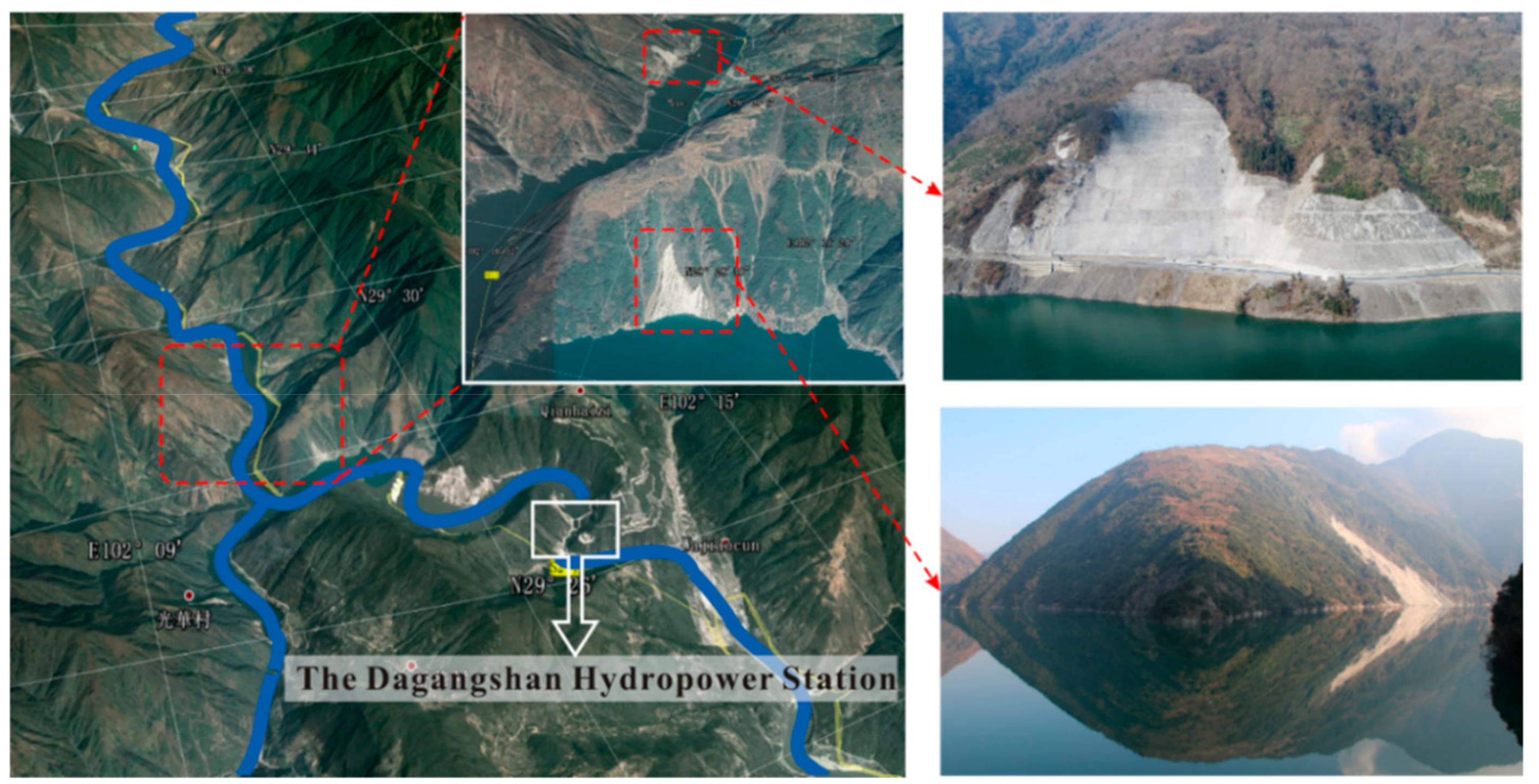
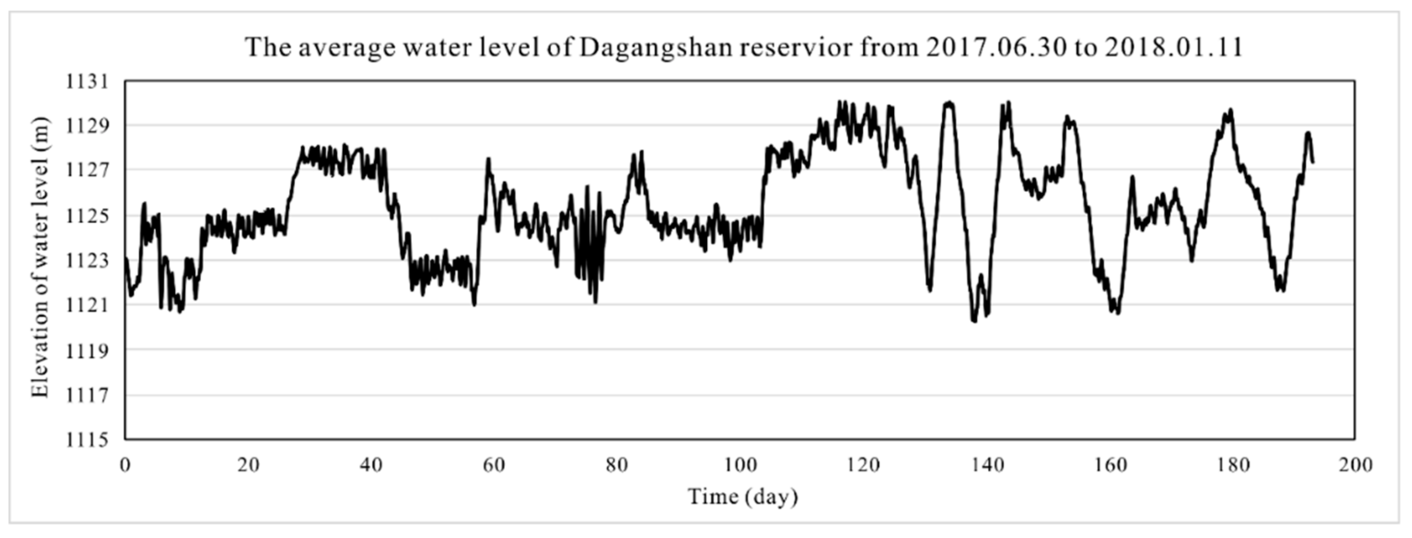
Frequent landslides have long motivated research into slope stability under various conditions [1,2,3,4,5,6,7,8,9]. Continuous research and field investigations have shown that geometric configuration is an important factor in the stability of both natural and constructed slopes [10,11,12,13,14,15]. However, the topographic effect on slope stability under fluctuating water conditions has rarely been investigated, even though slope deformation and instability occur frequently in reservoir areas [16,17,18,19,20,21,22]. As shown in Figure 1, with the Dagangshan Hydropower Station Reservoir area as an example, both the strike direction of the river and the slope angle around it change in a complex manner, often resulting in slope failures of different degrees. Moreover, the hydraulic conditions of the slopes in the reservoir area are very complex, as shown in Figure 2. On one hand, the poor properties of the slope mass cover layer reduce the overall slope stability, even for slope masses with reduced strength and complex seepage environments due to water level fluctuations [23]. On the other hand, most natural and constructed slopes exhibit a complex geometric configuration and three-dimensional (3D) state, which greatly increases the slope stability variability and calculation complexity. Coupled with the regular and sudden water level fluctuations, the topographic effect on slope stability considering saturated and unsaturated conditions urgently require research.
Slope stability analysis has been a research focus area for decades, using either the soil’s slide/column method based on the limit equilibrium concept, or the shear strength reduction method based on the finite element method [6,9]. The feasibility of 3D slope stability analysis has been proved to be a commonly used method today [24,25,26,27,28]. Moreover, with the continuous deepening of research, more powerful numerical techniques, like stronger technology of information gathering and processing, more realistic technology of numerical calculations, and smarter technology of monitoring and early warning, are required. The advanced numerical techniques have been proved to be a powerful tool to study both the failure stage and run-out of landslides [29,30,31,32,33]. Based on this research backdrop, considering the complex configuration of natural slopes, several studies were conducted to investigate how topographic factors (e.g., turning corner, slope gradient, turning arc, and convex- and concave-shaped surface geometry) affect slope stability under different boundary conditions [11,12,13,14,34,35]. From the researches above, one of the most important factors identified in slope stability is the constraining effect of the turning corner compared to that of general flat slopes, which will also be discussed in this study.
Similarly, many scholars have analyzed the stability of slopes subjected to various changes in the external water environment, water fluctuations or rainfall [16,17,36,37]. One key issue was the effect of water on slope stability, which was early quantified by Fredlund and Morgernstern [38] by considering the slope under different degrees of submergence and drawdown. From then on, slope stability with water effects gradually became a research hotspot. Former researches on saturated and unsaturated soils have provided better calculating methods for closer analysis of actual slope stability in this study using the 3D finite element method (FEM) with strength reduction technique. Lane and Griffiths [7] noticed that traditional analysis methods cannot cover the full range of possible critical conditions or adequately represent inhomogeneous slopes and complex loading arrangements. Thus, they proposed a chart-based operating safety approach by utilizing the finite element method to identify potentially critical conditions from rapid drawdown and partial submergence. Wheeler et al. [39] considered the significant influence of the degree of saturation on suction and the stress–strain behavior of unsaturated soil, and proposed a new elasto-plastic framework for unsaturated soils, involving coupling of hydraulic hysteresis and mechanical behavior. Griffith and Lu [40] presented results of unsaturated slope stability analyses using elasto-plastic finite elements in conjunction with a novel analytical formulation for the suction stress above the water table. Cai and Ugai [41] used the finite element analysis of transient water flow through unsaturated–saturated soils to investigate effects of hydraulic characteristics, the initial relative degree of saturation and the method with shear strength reduction technique to evaluate the stability of slopes under rainfall. Huang and Jia [42] discussed the utilization of the finite element method with the shear strength reduction technique approach in the stability analysis of soil slopes subjected to transient saturated/unsaturated seepage and presented the comparison of safety factors obtained from limited equilibrium method (LEM) and strength reduction FEM. It has been proved that the finite element method with the shear strength reduction technique was an effective method for assessing the safety factor of soil slopes under transient unsaturated seepage.
On the basis of previous research, the slope stability considering both saturated and unsaturated condition have been deeply carried out. For instance, as one of the greatest hydraulic engineering projects, the Three Gorges reservoir in China has drawn much attention worldwide. The geological structure and evolution of landslides subjected to water fluctuations in the reservoir area have been fully discussed since the reservoir’s impounding, using different types of methods, including limit equilibrium and finite element approaches [18,19,20,21]. Furthermore, Gao et al. [17] adopted a 3D rotational failure mechanism to investigate the influence of water drawdown on slope stability, and gave an example to demonstrate the difference in the safety factors obtained from 2D and 3D analyses. The results of this example indicated that the 3D effect can be neglected only when the slope has a large width (width to height ratio B/H ≥ 10.0).
These studies above showed that water fluctuations were an important factor in slope stability; in addition, the use of 3D analysis using the finite element method with strength reduction technique for different hydraulic conditions was validated. Meanwhile, field investigation and numerical simulation have become the most advantageous research methods. However, in engineering practice, the environment around the river or reservoir is complex. This requires additional attention, since slope deformation and instability in reservoir areas with varying geometric configurations and water levels occur frequently. In this study, the seepage, deformation and safety of slopes were analyzed using the finite element strength reduction method, considering both saturated and unsaturated slope mass conditions. Because soil parameters vary in engineering practice, the calculation models were set to be heterogeneous, including a cover layer with inferior properties. The topographic effects (surface shape, turning corner and slope gradient) on slope stability are then discussed in detail.
2. Methods
2.1. Fully Coupled Flow-Deformation Analysis
In previous studies, an effective stress–strain relationship was used to describe the mechanical behavior of saturated soil when the soil particles and water phase are assumed to be incompressible. However, soil behavior is highly nonlinear and irreversible, especially considering both saturated and unsaturated conditions with water level fluctuations [7,39,40,43]. In this study, a fully coupled flow-deformation analysis was conducted to analyze the simultaneous development of deformation and pore pressure in saturated and partially saturated soils as a result of time-dependent changes in the hydraulic boundary conditions. The fully coupled flow-deformation analysis considered the unsaturated soil behavior and the matric suction in the unsaturated zone above the phreatic level. The Soil Water Characteristic Curve (SWCC) proposed by Van Genuchten [44] was applied in this study to describe the hydraulic parameters of the groundwater flow in unsaturated zones, reflecting the soil’s capacity to keep water at different stresses. The Van Genuchten function is a three-parameter equation that relates the saturation to the pressure head Ψ:
where Pw is the suction pore stress; γw is the unit weight of the pore fluid; Sres is the residual saturation, which describes the part of the fluid that remains in the pores, even at high suction heads; Ssat is the saturation in a saturated situation, which defaults to 1.0; ga is a fitting parameter related to the soil’s air entry value, which must be measured for a specific material; gn is a fitting parameter which is a function of the rate of water extraction from the soil once the air entry value has been exceeded; gc is a fitting parameter that is used in the general Van Genuchten equation.
The deformation model applied in this study was formulated within the framework of continuum mechanics. The continuum description was discretized according to the finite element method. Each element consists of a number of nodes. Each node has a number of degrees of freedom that correspond to discrete values of the unknowns in the boundary value problem to be solved. In the present case of deformation theory, the degrees of freedom correspond to the displacement components. Subsequently, the slope stability was investigated using finite element analysis with the shear strength reduction technique, with the inputs of pore-water pressure and degree of saturation from the seepage analysis.
2.2. Strength Reduction Method
In previous studies, the limited equilibrium method (LEM) is the most extensive means for evaluating slope stability [45,46,47,48,49]. However, its difficult application to the finite element method, together with the failure mechanism assumptions, limited its development. This type of difficulty can be overcome by introducing a FEM with the shear strength reduction technique [7,50,51,52,53,54,55,56]. The strength reduction method (SRM) was first introduced in slope stability analysis by Zienkiewicz et al. [57], but was not widely applied due to the lack of finite element analysis procedures and strength criteria selection in the next few years [32,33,50,51,52,53,54,55,56]. With the development of computer technology and continued scholarly research, this SRM has gradually been recognized in stability analysis. Furthermore, SRM has taken stability analysis to a new level.
The shear strength reduction factor is defined as the ratio of the maximum shear strength of the slope mass to the actual shear stress generated by the external load while the external load remains unchanged. When the slope reaches the failure state, the displacement on the sliding surface will change abruptly, resulting in large and unlimited plastic flow and non-convergence in the finite element calculation. Therefore, the non-convergence of force and displacement is used as the failure criterion for the slope. The sliding failure surface (the area with a sudden change in plastic strain and displacement) can be obtained automatically, based on the elasto-plastic calculation results. Simultaneously, the safety factor (FS) can be determined. The process of solving for the safety factor can be simplified to the following formulas. The total multiplier ΣMsf is used to define the value of the soil strength parameters at a given stage in the analysis:
where the strength parameters with the subscript ‘input’ refer to the properties entered in the material sets, and parameters with the subscript ‘reduced’ refer to the reduced values used in the analysis. ΣMsf is set to 1.0 at the start of a calculation to set all material strengths to their input values. When slope failure occurs, the safety factor (FS) is given by:
2.3. Validation
Slope stability analysis has received scholarly attention for a long time. A typical slope model was used to verify the correctness of the calculations and settings. It was first proposed by Zhang [58] using an extended Spencer’s method, and has been widely used by various investigators, as part of the validation of their particular 3D slope stability methods [11,13,27,59,60,61,62,63]. In this study, a similar 3D model was established; the results are shown in Table 1. As shown, the result with the coarse mesh distribution model fits well with previous results; thus, the coarse form is used in the following analysis.
3. Numerical Model and Scheme
With the rapid development of computer hardware and numerical software, 3D slope analysis is gradually becoming mainstream for seepage, deformation and safety analysis [27,28]. In this paper, Plaxis 3D was used for numerical simulation. Furthermore, a fully coupled flow-deformation analysis was used to analyze the simultaneous development of deformation and pore pressure in saturated and partially saturated soil as a result of water fluctuations. The strength reduction method was used to determine global safety factors after a certain period of flow and deformation analysis. There were 27 different calculation conditions in this study, and the results are discussed in a later section.
3.1. Geometric Entities and Material Properties
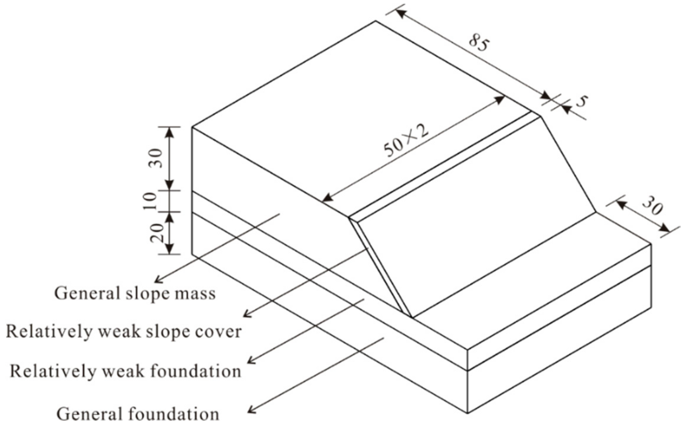
First, a general 3D slope model was constructed by extending the 2D model longitudinally. The geometric and soil information is given in Figure 3. The height of each slope was set to 30 m, and the bank slope subjected to water level fluctuations was divided into two identical 50-m long slopes by the axis of symmetry at the turning point. Considering the heterogeneity of slope soil and the inferior cover layer properties, the slope and foundation consist of two parts with poor and good soil conditions, respectively. The model has four different types of soil mass: the relatively weak cover layer, the general slope mass, the relatively weak foundation and the general foundation. The cover layer is 5 m thick. The general soil mass outside the turning corner range was set to at least 85 m in thickness to avoid the effect of water level fluctuations on the seepage field. There is no flow in the furthest soil mass by default. The foundation is a total of 30 m high, with a 10-m high relatively weak foundation.
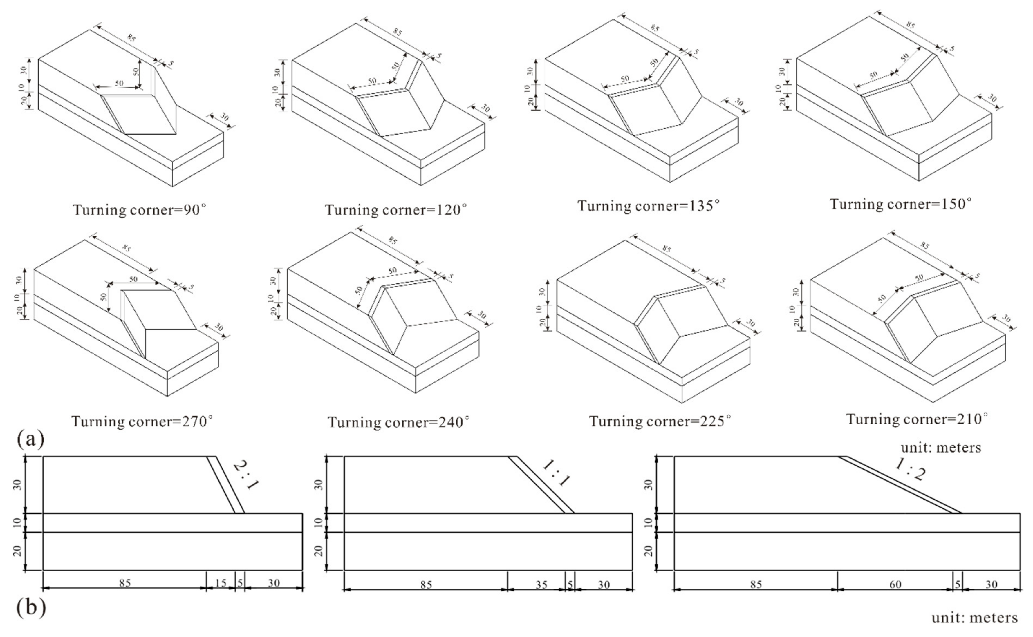
Three different slope gradients (2:1, 1:1 and 1:2 from steep to gentle, respectively) were investigated to determine the effect of slope gradient on stability. Meanwhile, nine different corner angles (90°, 120°, 135° and 150° with convex shapes, and 210°, 225°, 240° and 270° with concave shapes, along with 180° for comparison) were investigated with the three slope gradients above. The 27 calculation conditions in this study are shown in Figure 4. Each model was established with the same structural layering as the 2D extending model (180°). Table 2 shows the mass properties of each layer. A simplified selection of the most common soil types (coarse, medium, medium-fine, fine and very fine nonorganic material and organic material) based on the Hypres topsoil classification series [64] was adopted for subsequent use in the Van Genuchten model.
3.2. Mesh Generation and Boundary Conditions
After fully defining the model geometry, it was divided into finite elements for finite element calculations. However, previous studies have proven that the results from the finite element method with the strength reduction technique are sensitive to the design of the mesh [65]. Referring to the verification model of Zhang 1988 [58], the coarse element distribution results in this study (shown in Table 1) fit better with those of Zhang. Therefore, the overall model geometry was set to a coarse element distribution in this study. Furthermore, since the model geometry, including the edges, corners and structural objects, was complicated, the relatively weak layer required a finer finite element mesh. To balance the accurate numerical results of a sufficiently fine mesh against the excessive calculation times of very fine meshes, local refinement was used during mesh generation. A local coarseness factor was used to indicate the relative element size; the coarseness factor value set to 1.0 by default for most geometry entities. The cover layer was refined four times and the relatively weak foundation was refined 2 times. An example of the slope element distribution for a turning corner of 90° and a slope gradient of 1:2 is shown in Figure 5. The element distribution on the turning surface was much finer than that in distant areas.
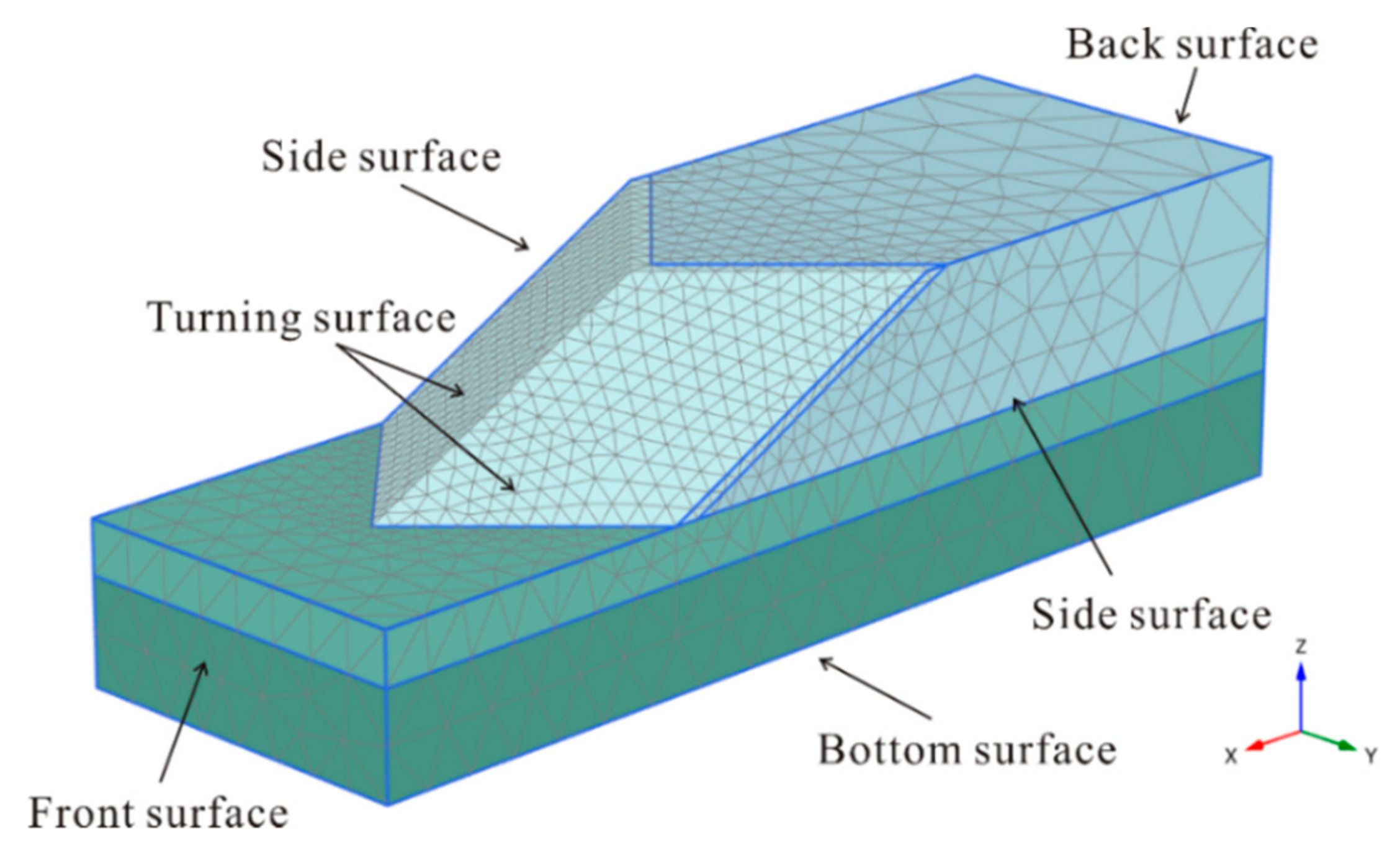
In addition, the boundary conditions assumed in the 3D numerical model were important; many scholars have investigated the boundary effects with different methods [27,28,66]. For a 3D slope with any complex shape, as shown in Figure 5, boundary surfaces generally fall into five categories (bottom surface, front surface, turning surface, back surface and side surface) [13]. In this study, all movements were restrained (in the normal, dip and strike directions) in the bottom plane of the model (i.e., ux, y, z = 0, where u is the displacement). The front surface and back surface were restrained in the normal direction, but free to move in the dip and strike directions. However, the boundary conditions for the side surfaces were flexible (generally classified into three types) as discussed in [11,12,13,27]. In this study, the side surface condition was set comparing the results and conclusions in previous studies. Combining the practices in the studied models, to reduce calculation time, the side surfaces were restrained only in the normal direction for the convex-shaped slopes (corner angles of 90°, 120°, 135° and 150°) to determine the actual slope failure mechanism. The side surfaces were completely restrained (in three directions) for concave-shaped slopes (with corner angles of 210°, 225°, 240° and 270°) to investigate the constraining effects of the turning corner and avoid a landslide near the side surfaces.
3.3. Hydraulic Conditions and Calculation Phases
After creating the model entity, a single borehole was established immediately to create a horizontal water surface (5 m as a regular condition) that extended to the model boundaries. The global water level then was specified as the established borehole water level to generate a simple hydrostatic pore pressure distribution (phreatic calculation type) for the full geometry. This global water level was used throughout the calculation process for the specific model. For the fluctuating water conditions, defining hydraulic conditions as groundwater flow boundary conditions was required. The specific hydraulic conditions have priority over global model conditions—if the global water level was used to define the hydraulic boundary conditions (groundwater head), the global water level would be replaced by the results of the groundwater flow calculation. In this study, the surface flow boundary conditions acting on the slope model’s turning surface were selected as the hydraulic conditions throughout the calculation process to meet the fluctuating water level conditions. The specific surface flow in each calculation phase is listed by calculation phase in a later section.
To build the calculation phases, a contrasting initial phase was established under the condition of regular water level without fluctuation before comparing the topographic effects on slope stability. A steady-state pore pressure with a 5-m water head was generated as the input for the initial phase, in which the calculation type was set to ‘Gravity loading’. The initial phase calculation determined the initial conditions of the pore water pressure and stress field, providing the basis for subsequent calculations. For the next condition (water rising), the time-dependent hydraulic boundary condition that water levels rise rapidly from 5 to 25 over 5 days was input before the transient groundwater flow analysis. The fully coupled flow-deformation analysis was selected for this phase to analyze the simultaneous development of deformation and pore water pressure in both saturated and unsaturated soils. Since the deformation due to gravity loading is physically meaningless, the ‘Reset displacements to zero’ option was chosen after ‘Gravity loading’ to remove these displacements. After the rapid water level rise, a five-day period of high water level was established to investigate the effect of pore water pressure due to infiltration. Similarly, the fully coupled flow-deformation analysis was selected for this and all later phases. The sharp drawdown of the water level was set to the same speed as that of the water rising (five days), after which a five-day period of low water level was established. The effects of the high water level infiltration and the low water level drainage are discussed later.
4. Results
Engineering practices have shown that geometric configurations have important effects on slope stability. To assess the topographic effect of the complicated terrain of different natural slopes on their stability under fluctuating water conditions, many numerical calculations were carried out. The three-dimensional geometric factors were simplified to different corner angles and slope gradients to control variables and build numerical calculation models. A total of 27 different conditions were analyzed using nine different corner angles (90°, 120°, 135° and 150° with convex shapes, 210°, 225°, 240° and 270° with concave shapes, along with 180° for comparison) and three different slope gradients (2:1, 1:1 and 1:2 for a very steep slope, a steep slope and a gentle slope, respectively). The above slope entities with different geometric conditions were simultaneously analyzed under different hydraulic conditions; the regular condition, water rising condition, water drawdown condition, and high and low water level conditions were evaluated.
4.1. Influence of Turning Corner
The turning corner of a natural 3D slope is one of the most representative geometric factors. Usually, convex-shaped and concave-shaped slopes will have different stability patterns, since they have different constraint effects.
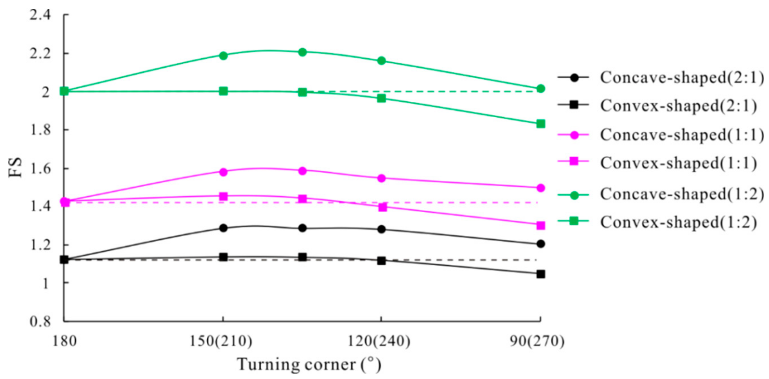
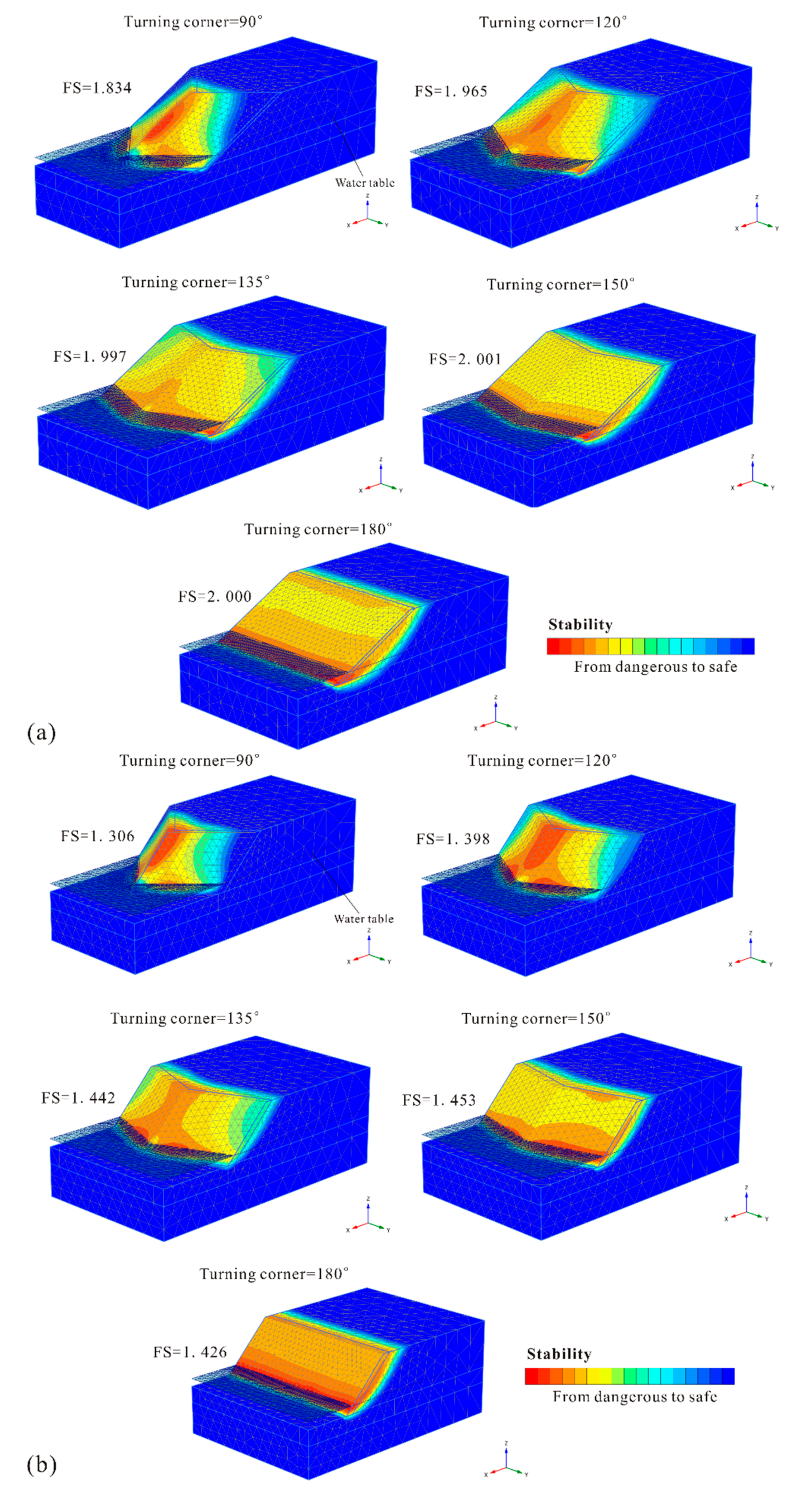
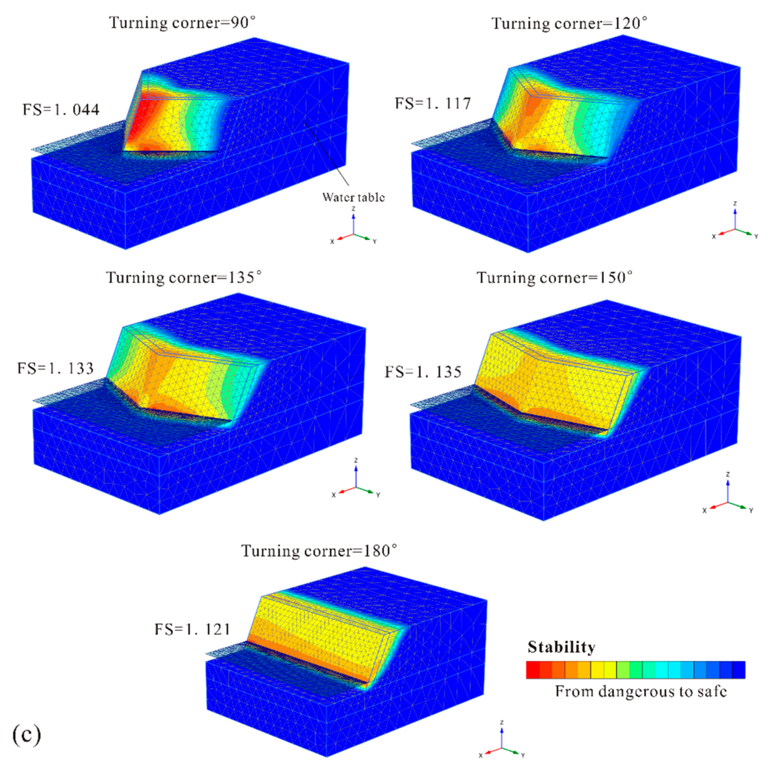
For convex-shaped slopes, Figure 6 shows the safety factors of slopes with corner angles were very near to or smaller than those of the 2D extended model (with a turning corner of 180°). The safety factor in the initial phase decreased as the slope turning corner value decreased from 150° to 90°, which indicates that a prominently exposed soil mass exhibits greater stability risks. Figure 7 shows the potential failure mechanism of each slope under regular hydraulic conditions with steady seepage. As shown, a diminishing turning corner gradually exposes the originally flat slope, which increases the slope instability. The smaller the turning corner, the thinner the exposed slope mass is. The convex-shaped slopes with corner angles of 150° and 135° are sufficiently large that they showed similar security as the 2D extending model (180°). The near-flat corner angles increase the volume of the potential landslide mass, which requires a greater external disturbance. Furthermore, a similar action of favorable boundary constraints due to the symmetric slope mass distribution may result in a slight increase in slope stability as the turning corner decreases from 180° to 150°. This confirms the effect of the boundary constraints from Nian et al. [11] and Zhang et al. [13]. Unfortunately, as the turning corner continues to decrease, the slope stability declines and drops sharply at 90°, as shown in Figure 6, resulting in the instability of thinner and smaller landslide masses in Figure 7. For convex-shaped slopes, the slightly favorable boundary constraints due to a convex symmetric slope mass distribution were not sufficient to offset the negative effects of slope exposure.
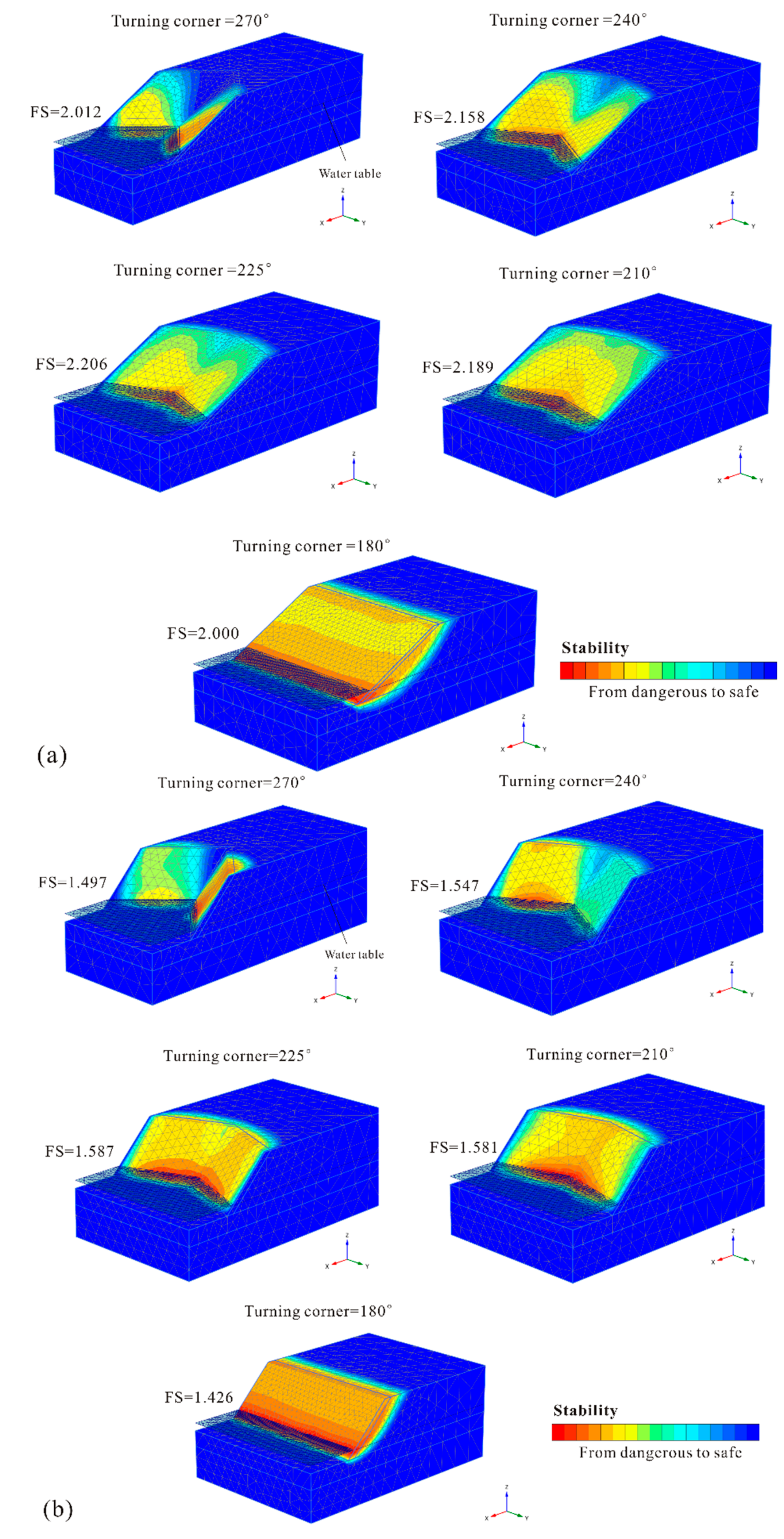
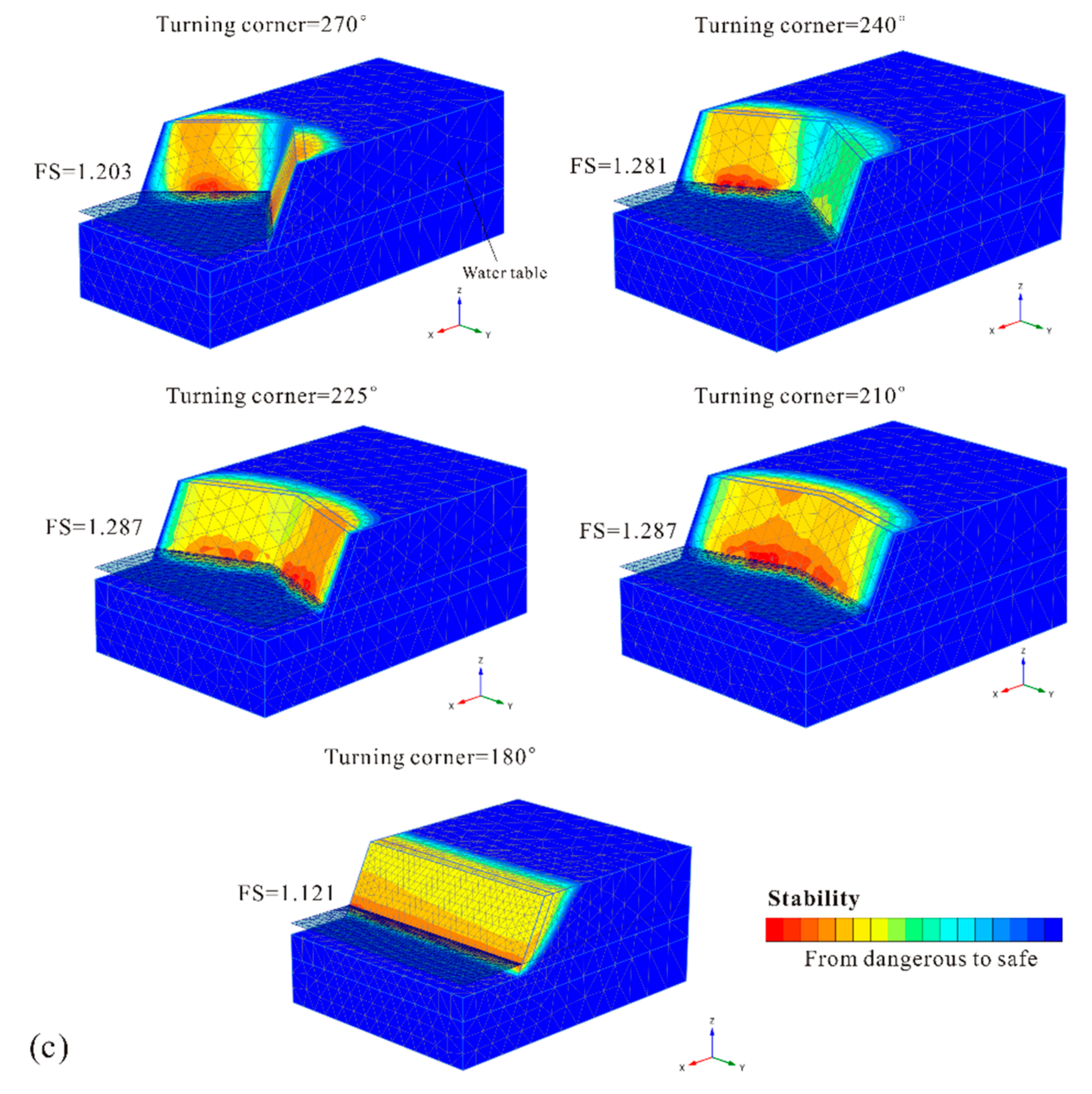
As is commonly known, a concave slope can provide beneficial constraints, with each part divided by the axis of symmetry. This contributes to the higher stability of slopes with corner angles. To prevent the formation of a landslide body from a thinner slope mass on the sides and determine the degree of the constraint effect, in this study, the deformation boundary conditions on both side surfaces were set to completely restrained in all three (normal, dip, and strike) directions. For concave-shaped slopes, as shown in Figure 6, regardless of the degree of increase of the slope security, whenever there was a turning corner, the stability increased compared to the 2D extending model (180°). This indicated significantly favorable boundary constraints due to the concave symmetric slope mass distribution. Figure 8 shows the potential failure mechanism of each slope under the regular hydraulic condition with steady seepage. As shown in Figure 6, similar to the convex-shaped slopes, concave slopes with corner angles of 150° and 135° had the highest stability, in stark contrast to other slopes with corner angles of 90° and 120°. Comparing the potential failure mechanism of the two slope types with different stabilities, it was found that the failure mass was divided into two parts by the axis of symmetry. This reduced the beneficial constraint effect due to the symmetrical distribution and further explained why the stability did not increase, but decreased, as the turning corner continued to decrease further.
4.2. Influence of the Slope Gradient
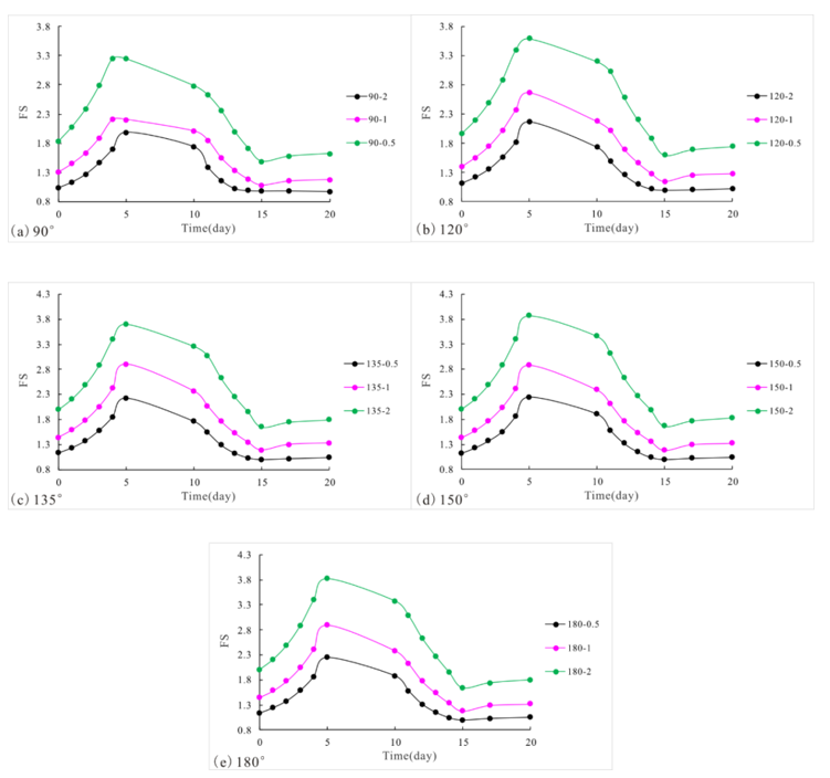
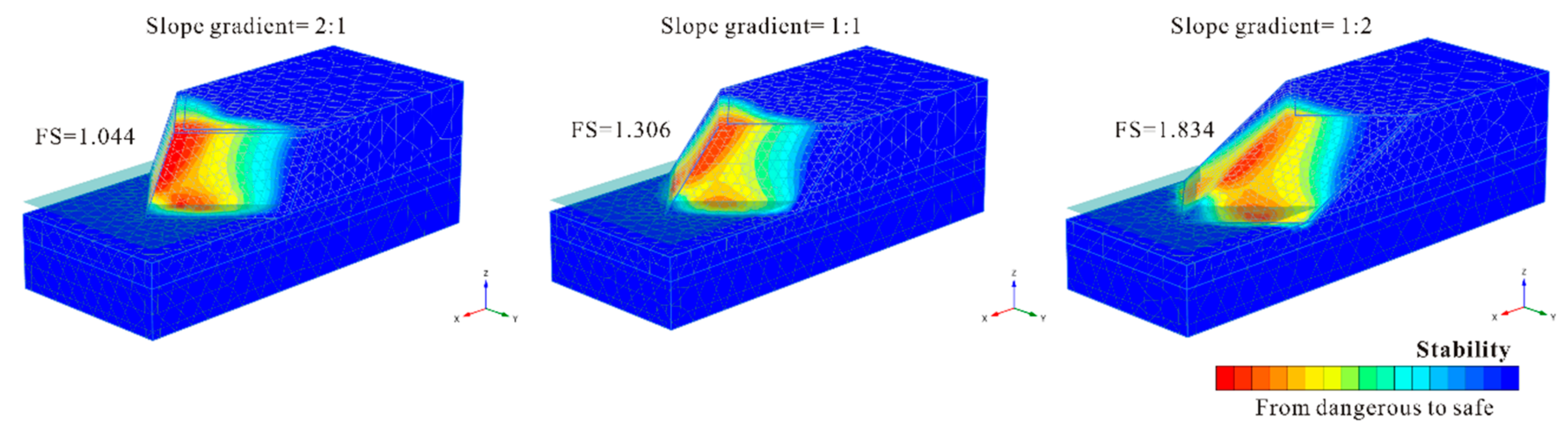
In this study, three slope gradients (2:1, 1:1, and 1:2 from steep to gentle, respectively) were calculated and analyzed successfully considering the unsaturated zone and conditions above the phreatic line. As shown in Figure 9, one routine conclusion was confirmed that the steeper the slope was, the lower the level of safety was. This result verifies the disturbance sensitivity of steep slope soil. Additionally, the safety factor variations of all three slope gradients in each water fluctuation time step are shown in Figure 9. Slopes with gentler gradients always had the highest stability at any point in the water fluctuations. Furthermore, the slope gradient did not have a significant effect on the safety factor variation pattern due to water fluctuations.
The most dangerous part of the potential failure mass is highlighted in Figure 10. The two areas that are most likely to slide in normal water level conditions were the most exposed mass on the axis of symmetry and the mass on the slope foot. Comparing the potential failure mechanism of the three slopes with 90° corner angles, the slip surface became deeper and wider as the slope gradient increased. This also confirms that stability drops sharply with increasing gradient.
4.3. Effect of Water Level Fluctuations
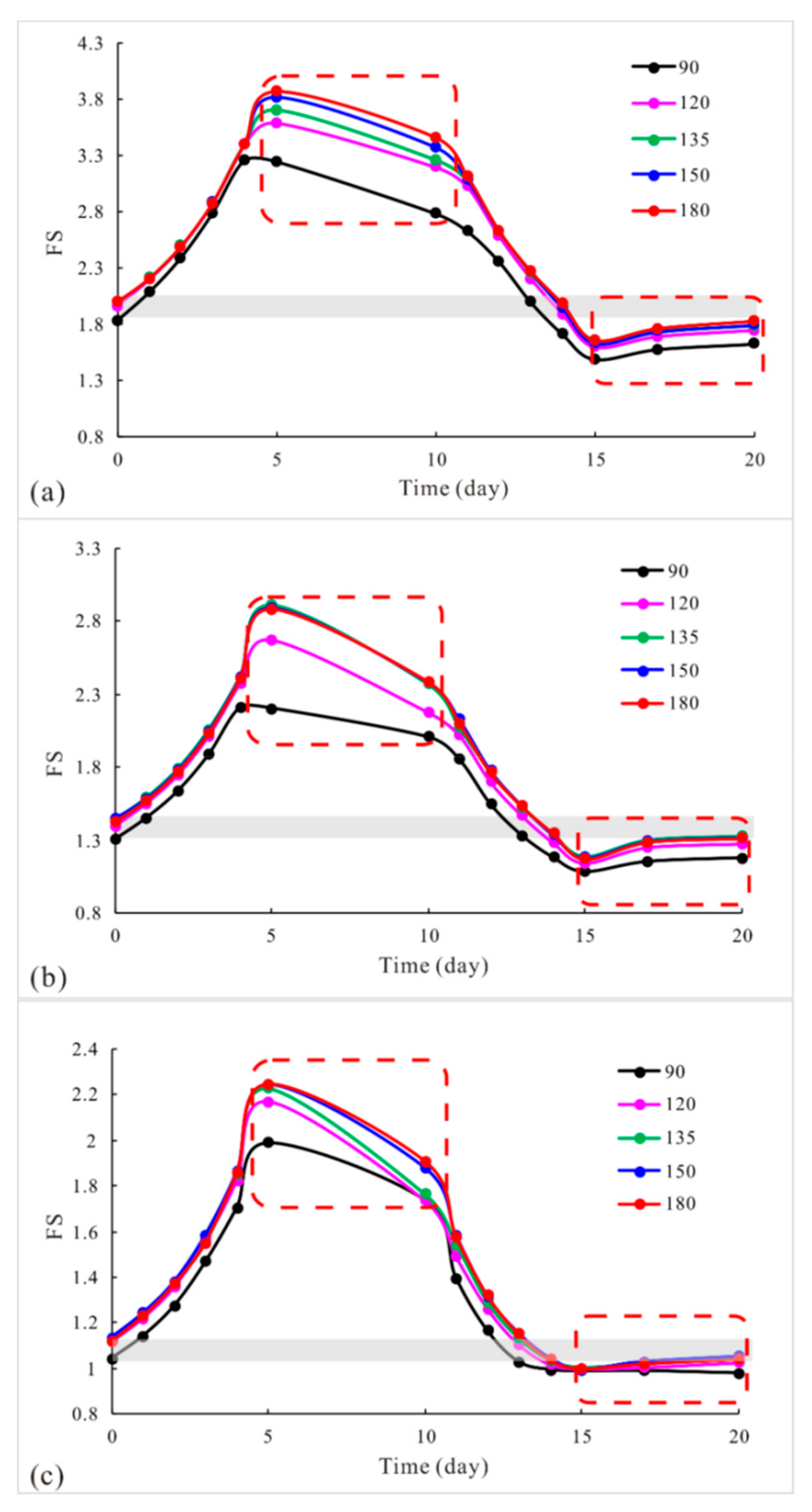
In engineering practice, water level fluctuation is a common phenomenon acting on the bank slope of the reservoir area. Regular water storage and drainage in reservoirs may cause slope instability, such as the landslides that occurred at the Three Gorges Reservoir area in China [16,17,18,19,20,21,22,23]. It is then conceivable that rapid water level fluctuations may lead to higher risks to slope deformation and stability. In this study, rapid rise and sharp drawdown water level fluctuation conditions were considered, with the continuous infiltration at the high water level and the successive slope drainage at the low water level. The slope mass safety factor was obtained for calculated time steps; the results are shown in Figure 11.
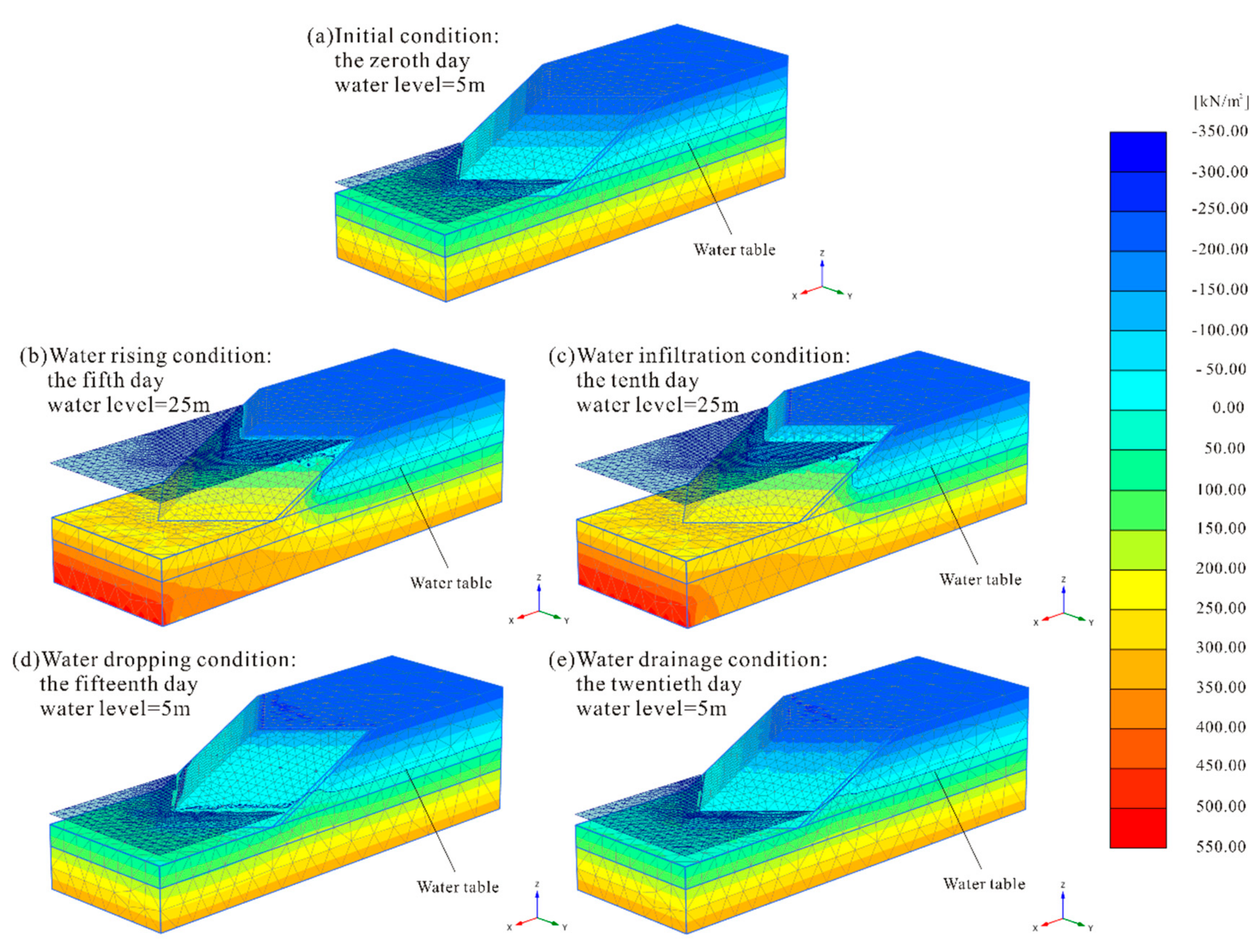
The pore water environment for different time steps is shown in Figure 12. In numerical calculation time, the zeroth day was set to calculate the seepage and stability of the bank slope for the normal water level condition considering steady-state groundwater flow. The slope calculation models remained stable initially. The rapid water level rise of 20 m was then set evenly from the first day to the fifth day under the transient (time-dependent) groundwater flow. Immediately after the rapid rise, a steady-state groundwater flow condition was assumed for the next five days (sixth to tenth days) considering continuous infiltration at a high water level. As shown in Figure 11, the stability increased as the water level rose, but decreased with continuous infiltration. The former result illustrates the beneficial effect of the water pressure acting as a back pressure. The latter result indicates the adverse effects of water infiltration caused by the increase in pore pressure. After a five-day high water level, from the eleventh day on, the water level dropped sharply for five days until the twentieth day, successively followed with a five-day drainage at the low water level. The slope stability decreased as the water level decreased, resulting in an even lower stability than the initial condition, due to the adverse effects of pore pressure. Thus, the slight increase in stability with the drainage of water over the next five days can be easily understood.
4.4. Variation of Slope Deformation
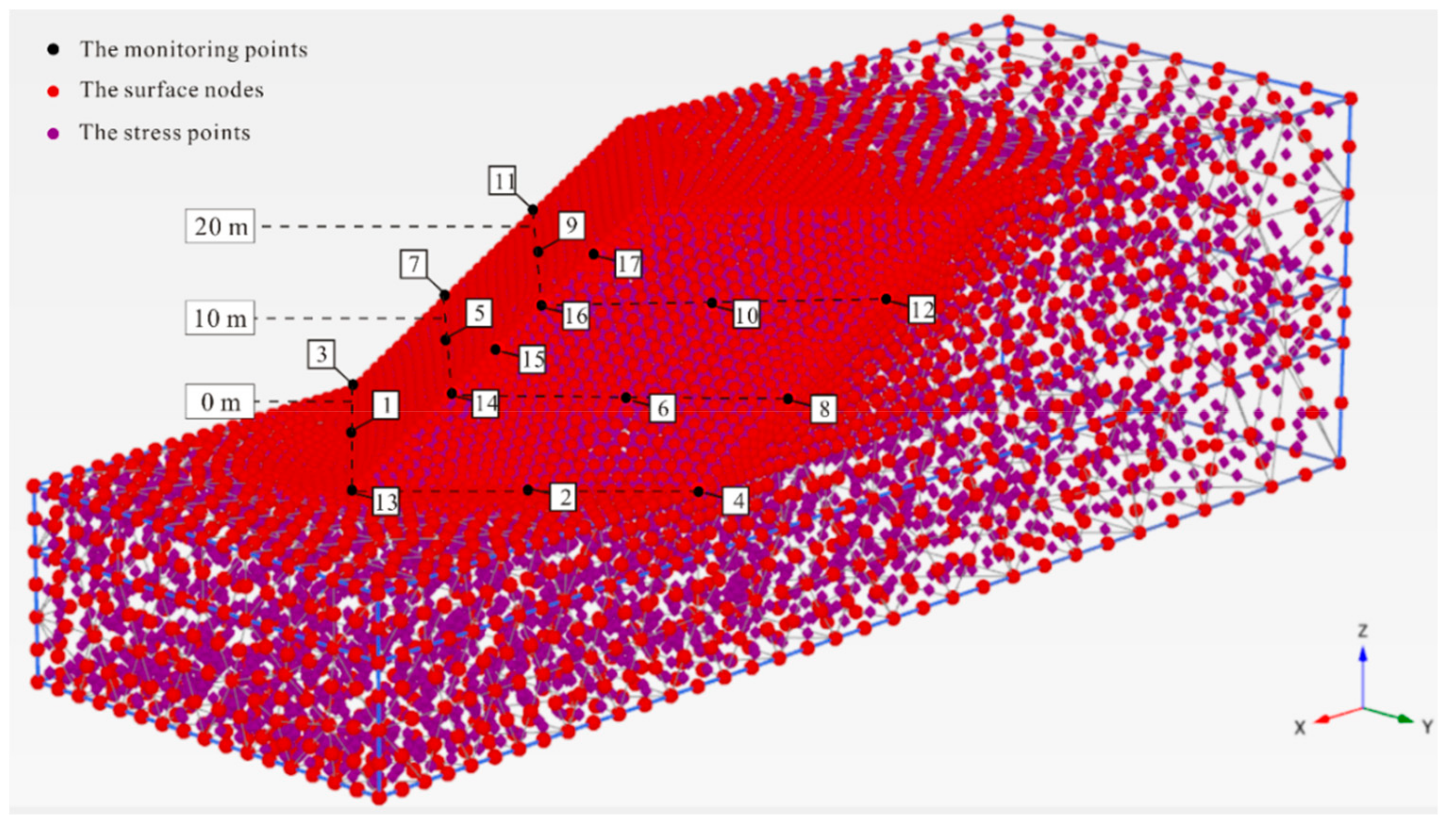
Figure 13 shows this study’s model calculation nodes. The model surfaces are represented by many nodes, and the stress points can be seen in the model body. The displacement data for 17 monitoring nodes were obtained. Their positions in the model are highlighted in Figure 13, representing the condition of the turning surface. Divided into two parts by the axis of symmetry, 5 columns of monitoring nodes on the turning surface were symmetrically distributed. Four columns of the nodes (nodes 1–12) were positioned on the outmost and the middle of the two surface parts, at heights of 0, 10 and 20 m, respectively. The remaining columns of nodes (node 13–17) were distributed on the model’s symmetry axis, at heights of 0, 10, 15, 20 and 25 m, respectively.
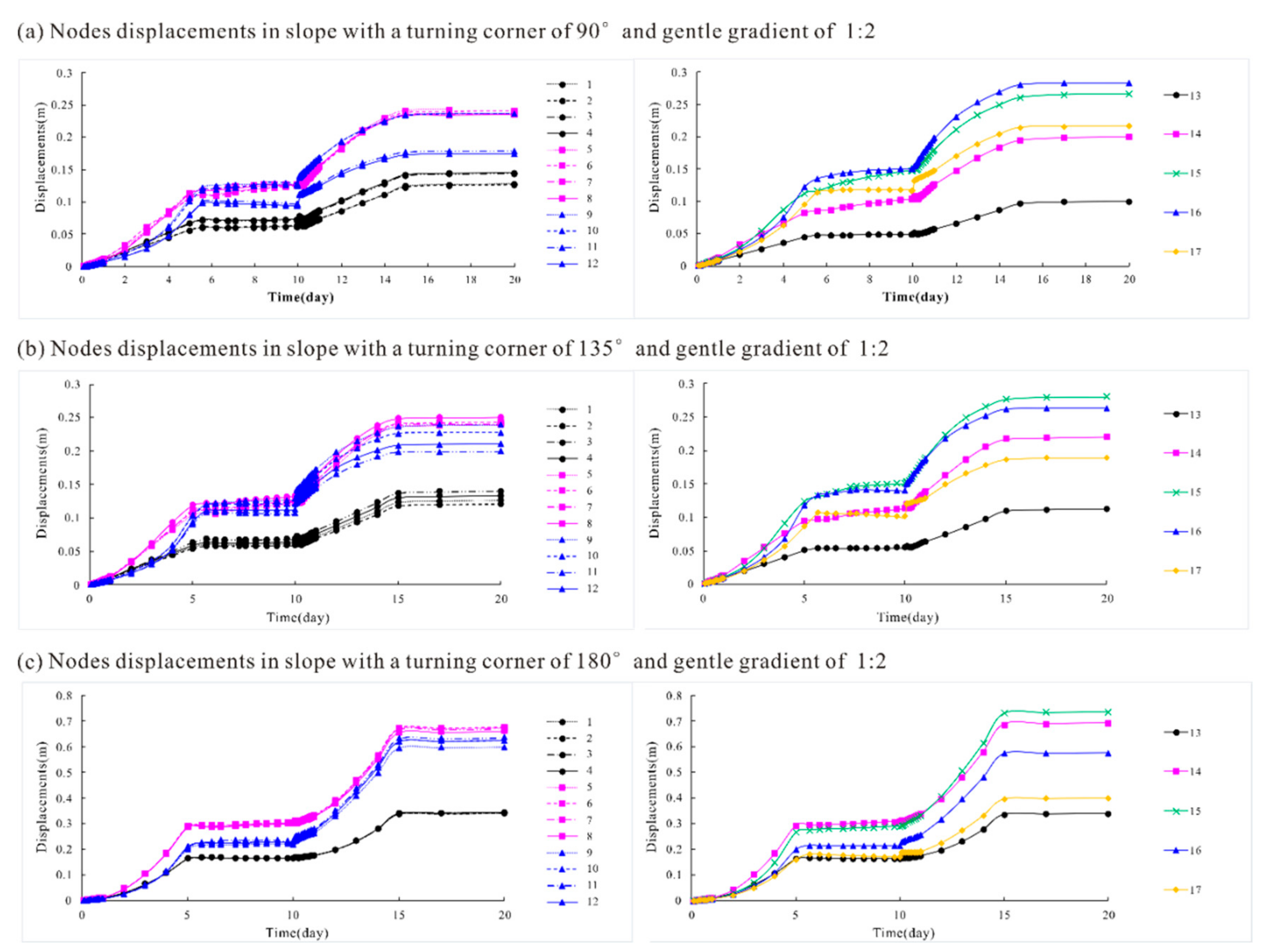
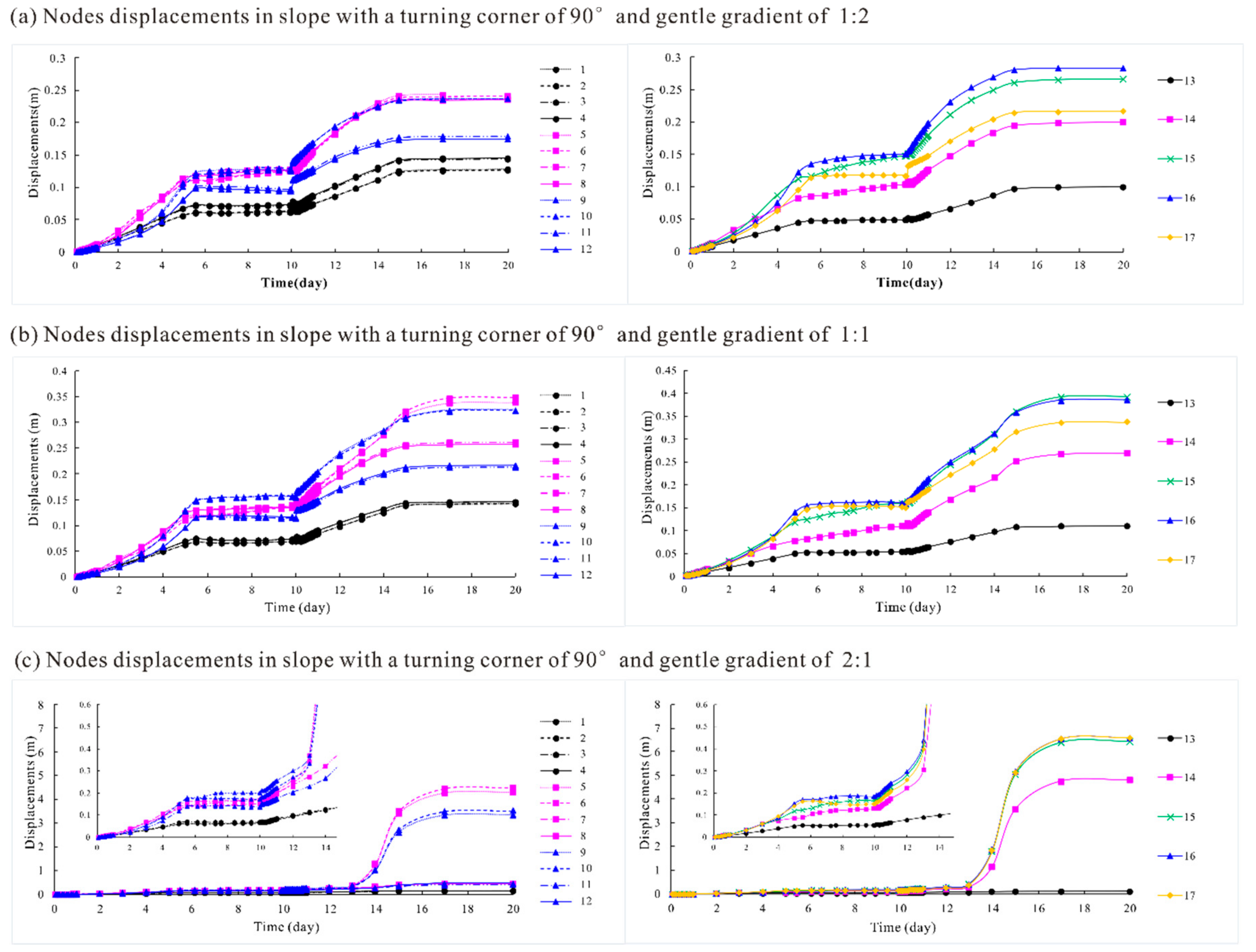
The obtained node displacements at each phase are shown in Figure 14 and Figure 15. The displacements of surface nodes are represented by different colors and icons for different heights (i.e., 0 m in white with ○, 10 m in pink with □, 15 m in green with ×, 20 m in blue with △, and 25 m in yellow with ◇), and different line types for different locations from the axis of symmetry. In general, the increasing trend of displacements with water level fluctuations was similar for all monitoring nodes. The general rule was that the node displacements increased rapidly during both the water level rise and fall processes, but increased very slowly as the water level remained unchanged.
As shown in Figure 14, the deformations of two nodes with a symmetric distribution were basically the same (i.e., deformations between nodes 1 and 2, nodes 3 and 4, nodes 5 and 6, nodes 7 and 8, nodes 9 and 10, and nodes 11 and 12). The deformations of nodes located different distances from the axis of symmetry and with different heights showed different changing characteristics for different turning corner values. One interesting phenomenon was the difference between the increasing trends of deformations for different turning corner values. Generally, when the water level was rising, the deformations increased slowly with a gradually increasing speed. However, the deformation increased rapidly with a gradually reducing speed for slopes with corner angles, while it increased rapidly with a gradually rising speed in 2D-extending slopes. Moreover, the location of the most dangerous part of the slope (i.e., the part with the largest deformation) was very different for slopes with different turning corner values. For a general shape slope (a 2D extending slope with a turning corner of 180°), the maximum deformation zone located lower, with a height of 10–15 m, while it located higher, at 15–20 m, on slopes with corner angles. This also confirms the slope failure mechanism shown in Figure 7 and Figure 8. The reason was probably that the failure of general slopes without corner angles often requires a large sliding mass, resulting in higher stability. The slipping surfaces of these slopes are usually located deeper and wider, with the maximum deformation zone located at a lower elevation. As shown in Figure 15, the increase in deformation for slopes with different gradients shows a similar pattern. However, the very steep slope of 2:1 with a turning corner of 90° failed when the water level dropped below 17 m during the 13th to 14th day of the water level fluctuations, manifesting as a dramatic increase in displacement.
4.5. Engineering Significance
For convex-shaped slopes, a turning corner usually has negative effects on stability, especially when the corner is relatively small and the thinner exposed slope mass greatly reduced the slope stability. Only when the turning corners were sufficiently large (150° to 135°) that they showed similar security as the 2D extending model (180°). In engineering practice, the slopes with small turning corners may be more unstable. In the reservoir area, under the influence of common water level fluctuations, those slopes are prone to deformation and even failure. Thus, the very small turning corner should be avoided (e.g., <120°). When it is necessary to learn the impact of other turning corners in different valves on stability, engineers can determine the range of influence based on the interpolation method with Figure 6.
For concave-shaped slopes, whatever the valve of the turning corner was, it always had a beneficial constraint effect on slope stability contributing to the symmetrical distribution. In engineering practice, the concave-shaped slopes may be more stable than other cases. However, the extremely small concave corner should also be avoided since the failure mass may be divided into two parts by the plane of symmetry and the beneficial constraint effect is likely to be reduced.
One routine conclusion was confirmed in this study that the steeper the slope is, the lower the safety factor, which means, the slopes with gentler gradients always had the highest stability. In engineering practice, the high and steep slopes usually show bad stability itself and prone to slope failure because of their sensitive responses to external interference. Although the stability of the gentler slope is always better, the engineer still needs to maintain the balance between the safety and economy of the project to determine the location and gradient of the slope. If necessary, measures such as slope protection and excavation can be taken.
5. Discussions
As is commonly known, there are few high and steep soil slopes in engineering practice. The poor physical and mechanical properties of soil mass and sensitive responses to the external interference, together with the slope configuration contribute to the failure of them. For stability analysis of high and steep soil slopes, when soil mass below the phreatic level was considered to be fully saturated, and suction effects in the soil above the phreatic level were ignored, the slope may calculated to have failed. Thus, in numerical calculation, a more realistic value of the safety factor will be obtained for stability analysis when suction is considered, where the suction acted as a positive value (tension) in the pore water pressure. This value is generally higher than a conventional safety factor ignoring suction, which also explains the successful calculation of high slope models with very steep gradients in this study. In calculation, the slope mass is divided into saturated and unsaturated zones by the phreatic line. When considering suction, the soil saturation depended on the soil-water retention curve, as defined in the corresponding material data sets. A saturation level was defined in the calculation by setting the water conditions to partially saturated; the resulting pore stress (suction) is calculated accordingly.
In this study, a comparison of the two cases (considering or ignoring suction) was conducted under the regular steady-state groundwater flow condition. To improve the calculation efficiency, 2D-extending models in three gradients were applied in this discussion. The effect of suction on stability can be simplified to the increase in effective cohesion [67]. As shown in Table 3, the condition of ignoring suction was carried out, and the assumed compensation effect of suction on effective cohesion was determined by increasing the safety factor of the calculation model to an equal level. It was confirmed that the suction in the partially saturated zone did have beneficial effects on slope stability. For a very steep slope (2:1), the FS was 1.121 considering suction. Unfortunately, when ignoring suction, the slope failed. In other words, this high and steep slope may not exist if calculated without considering suction. For a gentle slope, the effect of suction was approximately equal to a 10 kPa increment in effective cohesion, and 15 kPa for a steep slope, 25 kPa for a very steep slope. With an increasing slope gradient, the beneficial effects of suction increased, while the slope stability decreased.
Taking suction into consideration, the topographic effects on slope stability were studied under transient unsaturated seepage. Parametric analysis was conducted with the results of combinations of multiple configurations and varied hydraulic conditions. With generalizing the results of this study, some constructive suggestions can be directly adapted and used by other engineers. However, more research is still required for an accurate assessment of suction’s role in a partially saturated mass and the effects of more complex geometries on slope stability, which should be addressed in future studies.
6. Conclusions
In this study, a three-dimensional finite element strength reduction method was used to analyze the seepage, deformation and stability of slopes with different configurations. Combined with different soil parameters obtained from field investigation, the calculation models were established to be heterogeneous, with an inferior property cover layer. Considering both saturated and unsaturated zones of the slope mass, five hydraulic conditions varied with water level fluctuations (regular steady-state groundwater flow condition, water level rising and dropping conditions, high water level infiltration and low water level drainage) were conducted. Finally, the topographic effects (surface shape, turning corner and slope gradient) on slope stability were discussed from models with three different slope gradients (2:1, 1:1 and 1:2 from steep to gentle, respectively) and nine different corner angles (90°, 120°, 135° and 150° with convex shapes, and 210°, 225°, 240° and 270° with concave shapes, together with 180° for comparison). Based on the calculation results, the following conclusions are drawn.
(1) For convex-shaped slopes, the safety factor in the initial phase decreased as the slope turning corner decreased from 150° to 90°, indicating greater stability risks for the prominently exposed soil mass. The slope stability increases slightly from 180° to 150°, due to the favorable boundary constraints of the symmetric slope mass distribution, but these were not enough to offset the negative effects of the slope exposure.
(2) For concave-shaped slopes, whenever there was a turning corner, the stability significantly increased compared to the 2D extending model (180°). This indicated significantly favorable boundary constraints due to the concave symmetric slope mass distribution. However, the beneficial constraint effect of the symmetrical distribution was reduced for small corner angles (90–120°) because the failure mass was divided into two parts by the axis of symmetry.
(3) One routine conclusion was confirmed: the steeper the slope is, the lower the safety. Furthermore, the slope gradient did not significantly affect the safety factor variation pattern with water fluctuations; the slopes with gentler gradients always had the highest stability.
(4) The stability increased as the water level rose and decreased as the water level decreased, resulting in even lower stability than the initial condition due to the adverse effects of pore pressure. Conversely, stability decreased with continuous infiltration but increased slightly for a low water level with water drainage. The former result illustrates the beneficial effect of the water pressure acting as a back-pressure. The latter result indicates the adverse effects of water infiltration and the beneficial effects of water drainage, because of the variation in pore pressure.
(5) The node deformation increased rapidly during both water level rise and fall, but it increased very slowly as the water level remained unchanged. For a general shape slope (a 2D extending slope with a turning corner of 180°), the maximum deformation zone located lower, with a height of 10–15 m, while it located higher, at 15–20 m, for slopes with corner angles. Furthermore, some slopes failed when the water level dropped, manifesting as a dramatic displacement increase.
(6) In engineering practice, concave-shaped slopes always show better stability than that of convex-shaped slopes. Convex slopes with small turning corners should be avoided in engineering since they are prone to deformations and even landslides under the influence of common water level fluctuations. Meanwhile, the engineer needs to maintain the balance between safety and economy to determine the location and gradient of the slopes in engineering projects.
Author Contributions
Conceptualization, J.-W.Z.; methodology, Y.Z. and S.-C.Q.; validation, Y.Z., G.F. and M.-L.C.; investigation, G.F. and J.-W.Z.; resources, writing—original draft preparation, Y.Z.; writing—review and editing, S.-C.Q. and J.-W.Z.; funding acquisition, J.-W.Z. All authors have read and agreed to the published version of the manuscript.
Funding
This research was funded by the National Key R&D Program of China, grant number 2017YFC1501102 and the National Natural Science Foundation of China, grant number 41977229.
Acknowledgments
Critical comments by the anonymous reviewers greatly improved the initial manuscript.
Conflicts of Interest
The authors declare no conflicts of interest.
Data Availability Statement
The data used to support the findings of this study are available from the corresponding author upon request.
References
- Fellenius, W. Calculation of stability of earth dam. In Transactions, 2nd ed.; Congress Large Dams: Washington, DC, USA, 1936; Volume 4, pp. 445–462. [Google Scholar]
- Janbu, N. Application of composite slip surface for stability analysis. In Proceedings of the European Conference on Stability of Earth Slopes, Stockholm, Sweden, 20–25 September 1954; Volume 3, pp. 43–49. [Google Scholar]
- Hu, Y.X.; Yu, Z.Y.; Zhou, J.W. Numerical simulation of landslide-generated waves during the 11 October 2018 Baige landslide at the Jinsha River. Landslides 2020. [Google Scholar] [CrossRef]
- Morgenstern, N.R.; Price, V.E. The Analysis of the Stability of General Slip Surfaces. Géotechnique 1965, 15, 79–93. [Google Scholar] [CrossRef]
- Fredlund, D.G.; Krahn, J. Comparison of slope stability methods of analysis. Can. Geotech. J. 1977, 14, 429–439. [Google Scholar] [CrossRef]
- Griffiths, D.V.; Lane, P.A. Slope stability analysis by finite elements. Géotechnique 1999, 49, 387–403. [Google Scholar] [CrossRef]
- Lane, P.A.; Griffiths, D.V. Assessment of stability of slopes under drawdown conditions. J. Geotech. Geoenviron. Eng. 2000, 126, 443–450. [Google Scholar] [CrossRef]
- Zhu, D.Y.; Lee, C.F.; Jiang, H.D. Generalised framework of limit equilibrium methods for slope stability analysis. Géotechnique 2003, 53, 377–395. [Google Scholar] [CrossRef]
- Cheng, Y.M.; Lansivaara, T.; Wei, W.B. Two-dimensional slope stability analysis by limit equilibrium and strength reduction methods. Comput. Geotech. 2007, 34, 137–150. [Google Scholar] [CrossRef]
- Farzaneh, O.; Askari, F.; Ganjian, N. Three-dimensional stability analysis of convex slopes in plan view. J. Geotech. Geoenviron. Eng. 2008, 134, 1192–1200. [Google Scholar] [CrossRef]
- Nian, T.K.; Huang, R.Q.; Wan, S.S.; Chen, G.Q. Three-dimensional strength-reduction finite element analysis of slopes: Topographic effects. Can. Geotech. J. 2012, 49, 574–588. [Google Scholar] [CrossRef]
- Zhang, Y.; Chen, G.; Wang, B.; Li, L. An analytical method to evaluate the effect of a turning corner on 3D slope stability. Comput. Geotech. 2013, 53, 40–45. [Google Scholar] [CrossRef]
- Zhang, Y.; Chen, G.; Zheng, L.; Li, Y.; Zhuang, X. Effects of geometries on three-dimensional slope stability. Can. Geotech. J. 2013, 50, 233–249. [Google Scholar] [CrossRef]
- Ho, I.H. Parametric studies of slope stability analyses using three-dimensional finite element technique: Topographic effect. J. Geo-Eng. 2014, 9, 33–43. [Google Scholar]
- Zhou, J.W.; Xu, F.G.; Yang, X.G.; Yang, Y.C.; Lu, P.Y. Comprehensive analyses of the initiation and landslide-generated wave processes of the 24 June 2015 Hongyanzi landslide at the Three Gorges Reservoir, China. Landslides 2016, 13, 589–601. [Google Scholar] [CrossRef]
- Wang, H.B.; Xu, W.Y.; Xu, R.C.; Jiang, Q.H.; Liu, J.H. Hazard assessment by 3D stability analysis of landslides due to reservoir impounding. Landslides 2007, 4, 381–388. [Google Scholar] [CrossRef]
- Gao, Y.; Zhu, D.; Zhang, F.; Lei, G.H.; Qin, H. Stability analysis of three-dimensional slopes under water drawdown conditions. Can. Geotech. J. 2014, 51, 1355–1364. [Google Scholar] [CrossRef]
- Sun, G.; Zheng, H.; Tang, H.; Dai, F. Huangtupo landslide stability under water level fluctuations of the Three Gorges reservoir. Landslides 2016, 13, 1167–1179. [Google Scholar] [CrossRef]
- Wang, J.; Su, A.; Liu, Q.; Xiang, W.; Yeh, H.F.; Xiong, C.; Zou, Z.; Zhong, C.; Liu, J.; Cao, S. Three-dimensional analyses of the sliding surface distribution in the Huangtupo No. 1 riverside sliding mass in the Three Gorges Reservoir area of China. Landslides 2018, 15, 1425–1435. [Google Scholar] [CrossRef]
- Xiong, X.; Shi, Z.M.; Xiong, Y.L.; Ma, X.L.; Zhang, F. Prediction Method of Unsaturated Slope Stability under Rainfall and Fluctuation of Reservoir Water Level. In Proceedings of the GeoShanghai International Conference, Shanghai, China, 27–30 May 2018; Springer: Singapore, 2018; pp. 3–10. [Google Scholar]
- Wang, L.; Sun, D.A.; Li, L. 3D stability of partially saturated soil slopes after rapid drawdown by a new layer-wise sum. Landslides 2019, 16, 295–313. [Google Scholar] [CrossRef]
- Yan, L.; Xu, W.; Wang, H.; Wang, R.; Meng, Q.; Yu, J.; Xie, W.C. Drainage controls on the Donglingxing landslide (China) induced by rainfall and fluctuation in reservoir water levels. Landslides 2019, 16, 1583–1593. [Google Scholar] [CrossRef]
- Chen, M.L.; Lv, P.F.; Zhang, S.L.; Chen, X.Z.; Zhou, J.W. Time evolution and spatial accumulation of progressive failure for Xinhua slope in the Dagangshan reservoir, Southwest China. Landslides 2018, 15, 565–580. [Google Scholar] [CrossRef]
- Ugai, K.; Leshchinsky, D.O.V. Three-dimensional limit equilibrium and finite element analyses: A comparison of results. Soils Found. 1995, 35, 1–7. [Google Scholar] [CrossRef]
- Farzaneh, O.; Askari, F. Three-dimensional analysis of nonhomogeneous slopes. J. Geotech. Geoenviron. Eng. 2003, 129, 137–145. [Google Scholar] [CrossRef]
- Cheng, Y.M.; Yip, C.J. Three-Dimensional asymmetrical slope stability analysis extension of Bishop’s, Janbu’s, and Morgenstern–Price’s techniques. J. Geotech. Geoenviron. Eng. 2007, 133, 1544–1555. [Google Scholar] [CrossRef]
- Griffiths, D.V.; Marquez, R.M. Three-dimensional slope stability analysis by elasto-plastic finite elements. Géotechnique 2007, 57, 537–546. [Google Scholar] [CrossRef] [Green Version]
- Lin, H.D.; Wang, W.C.; Li, A.J. Investigation of dilatancy angle effects on slope stability using the 3D finite element method strength reduction technique. Comput. Geotech. 2020, 118, 103295. [Google Scholar] [CrossRef]
- Yan, Y.; Cui, Y.; Tian, X.; Hu, S.; Guo, J.; Wang, Z.; Yin, S.; Liao, L. Seismic signal recognition and interpretation of the 2019 “7.23” Shuicheng landslide by seismogram stations. Landslides 2020, 17, 1–16. [Google Scholar] [CrossRef]
- Yerro, A.; Soga, K.; Bray, J.D. Runout evaluation of Oso landslide with the material point method. Can. Geotech. J. 2019, 56, 1304–1317. [Google Scholar] [CrossRef] [Green Version]
- Conte, E.; Pugliese, L.; Troncone, A. Post-failure stage simulation of a landslide using the material point method. Eng. Geol. 2019, 253, 149–159. [Google Scholar] [CrossRef]
- Seyed-Kolbadi, S.M.; Sadoghi-Yazdi, J.; Hariri-Ardebili, M.A. An Improved Strength Reduction-Based Slope Stability Analysis. Geosciences 2019, 9, 55. [Google Scholar] [CrossRef] [Green Version]
- Wei, Y.; Jiaxin, L.; Zonghong, L.; Wei, W.; Xiaoyun, S. A strength reduction method based on the Generalized Hoek-Brown (GHB) criterion for rock slope stability analysis. Comput. Geotech. 2020, 117, 103240. [Google Scholar] [CrossRef]
- Zhang, F.; Gao, Y.; Leshchinsky, D.; Yang, S.; Dai, G. 3D effects of turning corner on stability of geosynthetic-reinforced soil structures. Geotext. Geomembr. 2018, 46, 367–376. [Google Scholar] [CrossRef]
- Zhang, F.; Leshchinsky, D.; Gao, Y.; Yang, S. Three-dimensional slope stability analysis of convex corner angles. J. Geotech. Geoenviron. Eng. 2018, 144, 06018003. [Google Scholar] [CrossRef]
- Simunek, J.; Van Genuchten, M.T.; Sejna, M. The HYDRUS Software Package for Simulating the Two-and Three-Dimensional Movement of Water, Heat, and Multiple Solutes in Variably-Saturated Media; Technical Manual, Version 1.0; PC Progress: Prague, Czech Republic, 2006; 241p. [Google Scholar]
- Conte, E.; Donato, A.; Pugliese, L.; Troncone, A. Analysis of the Maierato landslide (Calabria, Southern Italy). Landslides 2018, 15, 1935–1950. [Google Scholar] [CrossRef]
- Fredlund, D.G.; Morgenstern, N.R.; Widger, R.A. The shear strength of unsaturated soils. Can. Geotech. J. 1978, 15, 313–321. [Google Scholar] [CrossRef]
- Wheeler, S.J.; Sharma, R.S.; Buisson, M.S.R. Coupling of Hydraulic Hysteresis and Stress–strain Behavior in Unsaturated Soils. Géotechnique 2003, 53, 41–54. [Google Scholar] [CrossRef]
- Griffiths, D.V.; Lu, N. Unsaturated slope stability analysis with steady infiltration or evaporation using elasto-plastic finite elements. Int. J. Numer. Anal. Methods Geomech. 2005, 29, 249–267. [Google Scholar] [CrossRef]
- Cai, F.; Ugai, K. Numerical analysis of rainfall effects on slope stability. Int. J. Geomech. 2004, 4, 69–78. [Google Scholar] [CrossRef]
- Huang, M.; Jia, C.Q. Strength reduction FEM in stability analysis of soil slopes subjected to transient unsaturated seepage. Comput. Geotech. 2009, 36, 93–101. [Google Scholar] [CrossRef]
- Qi, S.; Vanapalli, S.K. Hydro-mechanical coupling effect on surficial layer stability of unsaturated expansive soil slopes. Comput. Geotech. 2015, 70, 68–82. [Google Scholar] [CrossRef]
- Van Genuchten, M.T. A closed-form equation for predicting the hydraulic conductivity of unsaturated soils 1. Soil Sci. Soc. Am. J. 1980, 44, 892–898. [Google Scholar] [CrossRef] [Green Version]
- Guo, C.X.; Cui, Y.F. Pore structure characteristics of debris flow source material in the Wenchuan earthquake area. Eng. Geol. 2020, 267, 105499. [Google Scholar] [CrossRef]
- Duncan, J.M. State of the art: Limit equilibrium and finite-element analysis of slopes. J. Geotech. Eng. 1996, 122, 577–596. [Google Scholar] [CrossRef]
- Li, A.J.; Merifield, R.S.; Lyamin, A.V. Limit analysis solutions for three dimensional undrained slopes. Comput. Geotech. 2009, 36, 1330–1351. [Google Scholar] [CrossRef]
- Liu, S.Y.; Shao, L.T.; Li, H.J. Slope stability analysis using the limit equilibrium method and two finite element methods. Comput. Geotech. 2015, 63, 291–298. [Google Scholar] [CrossRef]
- Sun, G.; Cheng, S.; Jiang, W.; Zheng, H. A global procedure for stability analysis of slopes based on the Morgenstern-Price assumption and its applications. Comput. Geotech. 2016, 80, 97–106. [Google Scholar] [CrossRef]
- Brinkgreve, R.B.J.; Bakker, H.L. Non-linear finite element analysis of safety factors. In Proceedings of the 7th International Conference on Computer Methods and Advances in Geomechanics, Cairns, Australia, 6–10 May 1991; pp. 1117–1122. [Google Scholar]
- Matsui, T.; San, K.C. Finite element slope stability analysis by shear strength reduction technique. Soils Found. 1992, 32, 59–70. [Google Scholar] [CrossRef] [Green Version]
- Dawson, E.M.; Roth, W.H.; Drescher, A. Slope stability analysis by strength reduction. Géotechnique 1999, 49, 835–840. [Google Scholar] [CrossRef]
- Fu, W.; Liao, Y. Non-linear shear strength reduction technique in slope stability calculation. Comput. Geotech. 2010, 37, 288–298. [Google Scholar] [CrossRef]
- Jiang, Q.; Qi, Z.; Wei, W.; Zhou, C. Stability assessment of a high rock slope by strength reduction finite element method. Bull. Eng. Geol. Environ. 2015, 74, 1153–1162. [Google Scholar] [CrossRef]
- Sun, C.; Chai, J.; Xu, Z.; Qin, Y.; Chen, X. Stability charts for rock mass slopes based on the Hoek-Brown strength reduction technique. Eng. Geol. 2016, 214, 94–106. [Google Scholar] [CrossRef]
- Nie, Z.; Zhang, Z.; Zheng, H. Slope stability analysis using convergent strength reduction method. Eng. Anal. Bound. Elem. 2019, 108, 402–410. [Google Scholar] [CrossRef]
- Zienkiewicz, O.C.; Humpheson, C.; Lewis, R.W. Associated and non-associated visco-plasticity and plasticity in soil mechanics. Géotechnique 1975, 25, 671–689. [Google Scholar] [CrossRef]
- Zhang, X. Three-dimensional stability analysis of concave slopes in plan view. J. Geotech. Eng. 1988, 114, 658–671. [Google Scholar]
- Lam, L.; Fredlund, D.G. A general limit equilibrium model for three-dimensional slope stability analysis. Can. Geotech. J. 1993, 30, 905–919. [Google Scholar] [CrossRef]
- Hungr, O. An extension of Bishop’s simplified method of slope stability analysis to three dimensions. Géotechnique 1987, 37, 113–117. [Google Scholar] [CrossRef]
- Huang, C.C.; Tsai, C.C.; Chen, Y.H. Generalized method for three-dimensional slope stability analysis. J. Geotech. Geoenviron. Eng. 2002, 128, 836–848. [Google Scholar] [CrossRef]
- Chen, Z.; Mi, H.; Zhang, F.; Wang, X. A simplified method for 3D slope stability analysis. Can. Geotech. J. 2003, 40, 675–683. [Google Scholar] [CrossRef]
- Chen, Z.; Wang, X.; Haberfield, C.; Yin, J.H.; Wang, Y. A three-dimensional slope stability analysis method using the upper bound theorem: Part I: Theory and methods. Int. J. Rock Mech. Min. Sci. 2001, 38, 369–378. [Google Scholar] [CrossRef]
- Wösten, J.H.M.; Lilly, A.; Nemes, A.; Le Bas, C. Development and use of a database of hydraulic properties of European soils. Geoderma 1999, 90, 169–185. [Google Scholar] [CrossRef]
- Shukha, R.; Baker, R. Mesh geometry effects on slope stability calculation by FLAC strength reduction method-linear and non-linear failure criteria. FLAC Numer. Model. Geomech. 2003, 2003, 109–116. [Google Scholar]
- Yu, Y.; Xie, L.; Zhang, B. Stability of earth–rockfill dams: Influence of geometry on the three-dimensional effect. Comput. Geotech. 2005, 32, 326–339. [Google Scholar] [CrossRef]
- Qi, S.; Vanapalli, S.K. Influence of swelling behavior on the stability of an infinite unsaturated expansive soil slope. Comput. Geotech. 2016, 76, 154–169. [Google Scholar] [CrossRef]
Figure 1.
The complex river flows in the upper reaches of the reservoir: the Dagangshan Hydropower Station.
Figure 1.
The complex river flows in the upper reaches of the reservoir: the Dagangshan Hydropower Station.

Figure 2.
The average water level of the Daganshan reservoir from 30 June 2017 to 11 January 2018.

Figure 3.
The 2D extending model for the studied slope.

Figure 4.
Calculating models with different corner angles and slope gradients: (a) different corner angles and (b) different slope gradients.
Figure 4.
Calculating models with different corner angles and slope gradients: (a) different corner angles and (b) different slope gradients.

Figure 5.
Element distribution in the 3D slope mass.

Figure 6.
Variation of safety factor with turning the corner under the initial condition.

Figure 7.
The failure mechanism of convex-shaped slopes with different corner angles: (a) gentle slope gradient of 1:2; (b) steep slope gradient of 1:1 and (c) very steep slope gradient of 2:1.
Figure 7.
The failure mechanism of convex-shaped slopes with different corner angles: (a) gentle slope gradient of 1:2; (b) steep slope gradient of 1:1 and (c) very steep slope gradient of 2:1.


Figure 8.
The failure mechanism of concave-shaped slopes with different corner angles: (a) gentle slope gradient of 1:2; (b) steep slope gradient of 1:1 and (c) very steep slope gradient of 2:1.
Figure 8.
The failure mechanism of concave-shaped slopes with different corner angles: (a) gentle slope gradient of 1:2; (b) steep slope gradient of 1:1 and (c) very steep slope gradient of 2:1.


Figure 9.
The difference in safety factor between slopes with three gradients: (a) turning corner = 90°; (b) turning corner = 120°; (c) turning corner = 135°; (d) turning corner = 150° and (e) turning corner = 180°.
Figure 9.
The difference in safety factor between slopes with three gradients: (a) turning corner = 90°; (b) turning corner = 120°; (c) turning corner = 135°; (d) turning corner = 150° and (e) turning corner = 180°.

Figure 10.
The difference in failure mechanism between slopes with three gradients: turning corner equal to 90°.
Figure 10.
The difference in failure mechanism between slopes with three gradients: turning corner equal to 90°.

Figure 11.
Variation of safety factor with water fluctuations: (a) gentle slope gradient of 1:2; (b) steep slope gradient of 1:1 and (c) very steep slope gradient of 2:1.
Figure 11.
Variation of safety factor with water fluctuations: (a) gentle slope gradient of 1:2; (b) steep slope gradient of 1:1 and (c) very steep slope gradient of 2:1.

Figure 12.
Variation of pore water pressure with water fluctuations: using an example slope with a turning corner of 90° and a gradient of 1:2: (a) initial condition; (b) water rising condition; (c) water infiltration condition; (d) water-dropping condition and (e) water drainage condition.
Figure 12.
Variation of pore water pressure with water fluctuations: using an example slope with a turning corner of 90° and a gradient of 1:2: (a) initial condition; (b) water rising condition; (c) water infiltration condition; (d) water-dropping condition and (e) water drainage condition.

Figure 13.
Distribution of nodes and stress points in the calculating model: an example using a slope with a turning corner of 90° and gradient of 1:2.
Figure 13.
Distribution of nodes and stress points in the calculating model: an example using a slope with a turning corner of 90° and gradient of 1:2.

Figure 14.
Monitoring node deformations for different corner angles with a gentle gradient of 1:2: (a) turning corner = 90°; (b) turning corner = 135° and (c) turning corner = 180°.
Figure 14.
Monitoring node deformations for different corner angles with a gentle gradient of 1:2: (a) turning corner = 90°; (b) turning corner = 135° and (c) turning corner = 180°.

Figure 15.
Deformations of monitoring nodes for different slope gradients with a small turning corner of 90°: (a) slope gradient = 1:2; (b) slope gradient = 1:1 and (c) slope gradient = 2:1.
Figure 15.
Deformations of monitoring nodes for different slope gradients with a small turning corner of 90°: (a) slope gradient = 1:2; (b) slope gradient = 1:1 and (c) slope gradient = 2:1.


Table 1.
Comparison of slope safety factors for validation.
| Source | Safety Factor (FS) | |
|---|---|---|
| Zhang (1988) [58] | 2.122 | |
| Chen et al. (2001) [63] | 2.262 | |
| Chen et al. (2003) [62] | 2.187 | |
| Griffiths and Marquez (2007) [27] | 2.170 | |
| Nian et al. (2012) [11] | 2.150 | |
| Zhang et al. (2013) [12] | 2.180 | |
| present study | very coarse | 2.194 |
| coarse | 2.139 | |
| medium | 2.085 | |
| fine | 2.049 | |
| very fine | 2.020 | |
Table 2.
Mass properties of each layer.
| Soil Mass | c (kN/m2) | φ (°) | γd (kN/m3) | γsat (kN/m3) | K (m/day) | E (kN/m2) | Ν (nu) |
|---|---|---|---|---|---|---|---|
| Cover layer | 15 | 30 | 17 | 19 | 0.1 | 10000 | 0.33 |
| General slope mass | 18 | 32 | 18 | 20 | 0.05 | 20000 | 0.33 |
| Relatively weak foundation | 10 | 35 | 17 | 21 | 0.015 | 50000 | 0.3 |
| General foundation | 15 | 38 | 18 | 22 | 0.01 | 50000 | 0.3 |
Table 3.
The comparison of the two cases considering or ignoring suction.
| Slope Gradient | Improved Effective Cohesion (kPa) | FS | |||||
|---|---|---|---|---|---|---|---|
| Cover Layer | General Slope Mass | Relatively Weak Foundation | General Foundation | Consider Suction | Ignore Suction | Improved | |
| Initial strength | 15 | 18 | 10 | 15 | |||
| 1:2 | 25 | 30 | 20 | 25 | 2.000 | 1.716 | 2.033 |
| 1:1 | 30 | 35 | 25 | 30 | 1.426 | 1.100 | 1.393 |
| 2:1 | 40 | 45 | 35 | 40 | 1.121 | — | 1.117 |
© 2020 by the authors. Licensee MDPI, Basel, Switzerland. This article is an open access article distributed under the terms and conditions of the Creative Commons Attribution (CC BY) license (http://creativecommons.org/licenses/by/4.0/).
Share and Cite
MDPI and ACS Style
Zhou, Y.; Qi, S.-C.; Fan, G.; Chen, M.-L.; Zhou, J.-W. Topographic Effects on Three-Dimensional Slope Stability for Fluctuating Water Conditions Using Numerical Analysis. Water 2020, 12, 615. https://doi.org/10.3390/w12020615
AMA Style
Zhou Y, Qi S-C, Fan G, Chen M-L, Zhou J-W. Topographic Effects on Three-Dimensional Slope Stability for Fluctuating Water Conditions Using Numerical Analysis. Water. 2020; 12(2):615. https://doi.org/10.3390/w12020615
Chicago/Turabian StyleZhou, Yue, Shun-Chao Qi, Gang Fan, Ming-Liang Chen, and Jia-Wen Zhou. 2020. "Topographic Effects on Three-Dimensional Slope Stability for Fluctuating Water Conditions Using Numerical Analysis" Water 12, no. 2: 615. https://doi.org/10.3390/w12020615
Note that from the first issue of 2016, this journal uses article numbers instead of page numbers. See further details here.